Approximation Properties of a New (p,q)-Post-Widder Operator

Abstract

We introduce a new $(p,q)$-Post-Widder operator along with its modified form which preserves the test functions $x^{\gamma },\gamma \in \mathbb{N}$. This paper aims to investigate the approximation properties of the $(p,q)$-Post-Widder operator while preserving $x^{\gamma }$. We estimate the convergence rate of the operators with the help of a continuity module and discuss their asymptotic behavior in terms of the weighted modulus of continuity. Also, our numerical results show that the new operator preserving $x^3$ provides the best approximation. In addition, we establish quantitative estimates of the difference between the two kinds of $(p,q)$-Post-Widder operators. Finally, using numerical examples and graphs, we illustrate that, for particular cases, our results provide improved convergence estimates.

1. Introduction

Classical Post-Widder operators [1,2] are defined by

$$P_n(f;x)={\displaystyle \frac{1}{n!}}{\int }_0^{\infty }f\left({\displaystyle \frac{xt}{n}}\right)t^n{e}^{-t}dt,x\in [0,\infty ),n\in \mathbb{N},$$

(1)

where $f\in C[0,\infty )$. These operators preserve linear functions but do not preserve the test functions $x^{\gamma }$, $\gamma =2,3,\cdots$. In order to obtain better approximation results, several researchers have proposed new constructions or modifications of operators. King [3] was the first to modify Bernstein operators to preserve the test functions 1 and $x^2$. Aldaz et al. [4] introduced a generalized classical Bernstein operator by fixing 1 and $x^{\gamma }$. Since then, several papers have been devoted to positive linear operators preserving polynomial functions. In order to preserve the test function $x^2$, Rempulska et al. [5] modified the Post-Widder operators proposed by May [6]. It was found that the modified form has improved approximation properties compared to the form in [6]. Then, Siddiqui et al. [7] studied a Voronovskaya-type theorem for these operators in polynomial-weighted spaces. After that, Gupta et al. [8,9], Srivastav et al. [10], and Abel et al. [11] dealt with modifications of the Post-Widder operators that preserve constant functions and $x^r$, where $r\in \mathbb{N}$.

With the development of q-calculus and symmetric q-calculus, a number of q-analogues of linear positive operators have been constructed and extensively discussed. As usual, for a nonnegative integer n, q-number ${\left[n\right]}_q$, q-factorial, and the improper q-integral of $f\left(x\right)$ on $[0,\infty )$ (see [12]) are defined as follows

$$\begin{array}{cc}\hfill {\left[n\right]}_q& ={\displaystyle \frac{1-q^n}{1-q}},0<q<1;{\left[n\right]}_0=1,\hfill \\ \hfill {\left[n\right]}_q!& =\prod _{k=1}^n{\left[k\right]}_q,n\ge 1;{\left[0\right]}_{p,q}!=1,\hfill \\ \hfill {\int }_0^{a}f\left(x\right)d_{q}x& =a(1-q)\sum _{n=0}^{\infty }f\left(a{q}^n\right)q^n,a>0.\hfill \end{array}$$

(2)

Also, the q-exponential functions (see [13]) are defined by $E_q\left(x\right)={\displaystyle \sum _{n=0}^{\infty }}{\displaystyle \frac{q^{\left(\genfrac{}{}{0pt}{}{n}{2}\right)}}{{\left[n\right]}_q!}}{x}^n$. In 2012, Ünal et al. [14] introduced a q-Post-Widder operator for $q\in (0,1)$, as follows:

$$P_{n,q}(f;x)={\displaystyle \frac{1}{{\left[n\right]}_q!}}{\int }_0^{{\displaystyle \frac{1}{1-q}}}f\left({\displaystyle \frac{xt}{{\left[n\right]}_q}}\right)t^n{E}_q(-qt)d_{q}t,x\in [0,\infty ),$$

(3)

where $f\in C_B[0,\infty )$, which denotes the space of all bounded and continuous functions on $[0,\infty )$ endowed with the norm $\parallel f\parallel =\underset{[0,\infty )}{sup}\left|f\left(x\right)\right|$. They studied the statistical approximation properties of real and complex q-Post-Widder operators. It can be easily seen that for $q\to 1^{-}$, the operators in (3) are classical Post-Widder operators (1). Recently, the theory of positive linear operators has been intensively applied in post-quantum calculus ($(p,q)$-calculus), which has been studied extensively in various fields such as physical sciences, differential equations, and combinatorics. A $(p,q)$-analogue of the Bernstein operators was first introduced by Mursaleen [15]. Since then, $(p,q)$-analogues of operators have been intensively investigated by many researchers (see [16,17,18,19,20]). Let us recall and introduce some concepts from $(p,q)$-calculus (see [21]).

For a nonnegative integer n, $(p,q)$-number ${\left[n\right]}_{p,q}$ and $(p,q)$-factorial ${\left[n\right]}_{p,q}!$ are defined by

$$\begin{array}{cc}\hfill {\left[n\right]}_{p,q}& ={\displaystyle \frac{p^n-q^n}{p-q}},0<q<p\le 1,\hfill \\ \hfill {\left[n\right]}_{p,q}!& =\prod _{k=1}^n{\left[k\right]}_{p,q},n\ge 1;{\left[0\right]}_{p,q}!=1.\hfill \end{array}$$

(4)

The improper $(p,q)$-integral of $f\left(x\right)$ on $[0,\infty )$ is given by

$${\int }_0^{\infty }f\left(x\right)d_{p,q}x=(p-q)\sum _{j=-\infty }^{\infty }{\displaystyle \frac{q^j}{p^{j+1}}}f\left({\displaystyle \frac{q^j}{p^{j+1}}}\right),0<{\displaystyle \frac{q}{p}}<1.$$

(5)

Further, two $(p,q)$-exponential functions are defined as follows

$$\begin{array}{cc}\hfill e_{p,q}\left(x\right)& =\sum _{n=0}^{\infty }{\displaystyle \frac{p^{\left(\genfrac{}{}{0pt}{}{n}{2}\right)}}{{\left[n\right]}_{p,q}!}}{x}^n,\hfill \\ \hfill E_{p,q}\left(x\right)& =\sum _{n=0}^{\infty }{\displaystyle \frac{q^{\left(\genfrac{}{}{0pt}{}{n}{2}\right)}}{{\left[n\right]}_{p,q}!}}{x}^n.\hfill \end{array}$$

(6)

We know that $e_{p,q}\left(x\right)·E_{p,q}(-x)=1$ (see [21,22]). The $(p,q)$-Gamma function (see [21]) is given as

$${\gamma }_{p,q}\left(x\right)=p^{{\displaystyle \frac{n(n-1)}{2}}}{\int }_0^{\infty }{t}^{x-1}{E}_{p,q}(-qt)d_{p,q}t.$$

(7)

The following identity holds true:

$${\gamma }_{p,q}(n+1)={\left[n\right]}_{p,q}!.$$

(8)

In [23], Mishra et al. introduced a modified $(p,q)$-Baskakov operator, which reproduces $x^2$. Then, Cheng et al. [24] constructed and investigated $(p,q)$-gamma operators that preserve the test function $x^2$. These results motivated us to construct a new $(p,q)$-Post-Widder operator preserving 1 and $x^{\gamma }$ for $\gamma \in \mathbb{N}$. In this paper, firstly, we propose the following $(p,q)$-Post-Widder linear positive operators

$$P_n^{p,q}(f;x):={\displaystyle \frac{1}{{\Gamma }_{p,q}(n+1)}}{\int }_0^{\infty }f\left({\displaystyle \frac{p^{n}xt}{{\left[n\right]}_{p,q}}}\right)p^{{\displaystyle \frac{n(n+1)}{2}}}{t}^n{E}_{p,q}(-qt)d_{p,q}t.$$

(9)

where $f\in C[0,\infty )$, $0<q<p\le 1$. When $p=1$, the operators $P_n^{p,q}$ reduce to the q-Post-Widder operators (3). The operators (9) preserve constant functions only. In order to preserve the test functions $x^{\gamma }$, we define a new modification of operator (9), i.e.,

$${\mathbf{P}}_{n,\gamma }^{p,q}(f;x):={\displaystyle \frac{1}{{\Gamma }_{p,q}(n+1)}}{\int }_0^{\infty }f\left({\displaystyle \frac{p^n{\theta }_{n,\gamma }\left(x\right)t}{{\left[n\right]}_{p,q}}}\right)p^{{\displaystyle \frac{n(n+1)}{2}}}{t}^n{E}_{p,q}(-qt)d_{p,q}t,$$

(10)

where

$${\theta }_{n,\gamma }\left(x\right)={\displaystyle \frac{p^{\frac{\gamma +1}{2}}{\left[n\right]}_{p,q}}{{\left({[n+1]}_{p,q}\right)}_{\gamma }^{\frac{1}{\gamma }}}}x,$$

(11)

${\left({\left[n\right]}_{p,q}\right)}_{\gamma }={\left[n\right]}_{p,q}{[n+1]}_{p,q}\cdots {[n+\gamma -1]}_{p,q}$, ${\left({\left[n\right]}_{p,q}\right)}_0=1$. It is clear that

$${\mathbf{P}}_{n,\gamma }^{p,q}(f;x)=P_n^{p,q}\left(f;{\theta }_{n,\gamma }\left(x\right)\right).$$

(12)

Thus, the modified operator ${\mathbf{P}}_{n,\gamma }^{p,q}$ preserves the constant function as well as $x^{\gamma }$. Moreover, we study the moments of the operators $P_n^{p,q}$ and ${\mathbf{P}}_{n,\gamma }^{p,q}$ in Section 2. In Section 3, we present the approximation properties of the modified operators ${\mathbf{P}}_{n,\gamma }^{p,q}$ using the modulus of continuity, Peetre’s K-functional, and the weighted modulus of continuity. We deduce that these operators (10) provide a better approximation for $\gamma =3$. In Section 4, we obtain the estimates of the difference between the two operators. Finally, we compare the convergence rate and error estimation of the operators ${\mathbf{P}}_{n,\gamma }^{p,q}$ with $P_n^{p,q}$ using numerical examples. We show that our modified operator ${\mathbf{P}}_{n,\gamma }^{p,q}$ provides an improved estimation in some sense.

2. Preliminary Results

Lemma 1.

Let $e_{\nu }\left(t\right)=t^{\nu }$, $\nu \in N_0$. Then,

$$P_n^{p,q}(e_{\nu };x)={\displaystyle \frac{p^{-\frac{\nu (\nu +1)}{2}}{[n+\nu ]}_{p,q}!}{{\left[n\right]}_{p,q}^{\nu }{\left[n\right]}_{p,q}!}}{x}^{\nu }={\displaystyle \frac{p^{-\frac{\nu (\nu +1)}{2}}{\left({[n+1]}_{p,q}\right)}_{\nu }}{{\left[n\right]}_{p,q}^{\nu }}}{x}^{\nu }.$$

(13)

Proof. 

Using (7) and (8), we have

$$\begin{array}{cc}\hfill P_n^{p,q}(e_{\nu };x)& ={\displaystyle \frac{1}{{\Gamma }_{p,q}(n+1)}}{\int }_0^{\infty }{\left({\displaystyle \frac{p^{n}xt}{{\left[n\right]}_{p,q}}}\right)}^{\nu }{p}^{{\displaystyle \frac{n(n+1)}{2}}}{t}^n{E}_{p,q}(-qt)d_{p,q}t\hfill \\ \hfill & ={\displaystyle \frac{x^{\nu }{p}^{-\frac{\nu (\nu +1)}{2}}}{{\left[n\right]}_{p,q}^{\nu }{\Gamma }_{p,q}(n+1)}}{\int }_0^{\infty }{p}^{{\displaystyle \frac{(n+\nu )(n+\nu +1)}{2}}}{t}^{\nu +n}{E}_{p,q}(-qt)d_{p,q}t\hfill \\ \hfill & ={\displaystyle \frac{x^{\nu }{p}^{-\frac{\nu (\nu +1)}{2}}}{{\left[n\right]}_{p,q}^{\nu }{\Gamma }_{p,q}(n+1)}}{\Gamma }_{p,q}(n+\nu +1)\hfill \\ \hfill & ={\displaystyle \frac{p^{-\frac{\nu (\nu +1)}{2}}{[n+\nu ]}_{p,q}!}{{\left[n\right]}_{p,q}^{\nu }{\left[n\right]}_{p,q}!}}{x}^{\nu }={\displaystyle \frac{p^{-\frac{\nu (\nu +1)}{2}}{\left({[n+1]}_{p,q}\right)}_{\nu }}{{\left[n\right]}_{p,q}^{\nu }}}{x}^{\nu }.\hfill \end{array}$$

□

Following (10)–(12), the modified $(p,q)$-Post-Widder operators ${\mathbf{P}}_{n,\gamma }^{p,q}$ can be expressed as

$${\mathbf{P}}_{n,\gamma }^{p,q}(f;x)={\displaystyle \frac{1}{{\Gamma }_{p,q}(n+1)}}{\int }_0^{\infty }f\left({\displaystyle \frac{p^{\frac{2n+\gamma +1}{2}}xt}{{\left({[n+1]}_{p,q}\right)}_{\gamma }^{\frac{1}{\gamma }}}}\right)p^{{\displaystyle \frac{n(n+1)}{2}}}{t}^n{E}_{p,q}(-qt)d_{p,q}t.$$

(14)

Combining the Lemma 1 and (14), we derive the $\nu$-th order moments of operators ${\mathbf{P}}_{n,\gamma }^{p,q}$ as follows.

Lemma 2.

For $x\in [0,\infty )$, we have

$${\mathbf{P}}_{n,\gamma }^{p,q}(e_{\nu };x)={\displaystyle \frac{{\left({[n+1]}_{p,q}\right)}_{\nu }}{p^{\frac{\nu (\nu +1)}{2}}{\left[n\right]}_{p,q}^{\nu }}}{\theta }_{n,\gamma }^{\nu }\left(x\right)={\displaystyle \frac{p^{\frac{\nu (\gamma -\nu )}{2}{\left({[n+1]}_{p,q}\right)}_{\nu }}}{{\left({[n+1]}_{p,q}\right)}_{\gamma }^{\frac{\nu }{\gamma }}}}{x}^{\nu }.$$

(15)

Some initial moments are

$$\begin{array}{cc}\hfill {\mathbf{P}}_{n,\gamma }^{p,q}(1;x)& =1,\hfill \\ \hfill {\mathbf{P}}_{n,\gamma }^{p,q}(t;x)& ={\displaystyle \frac{{[n+1]}_{p,q}}{p{\left[n\right]}_{p,q}}}{\theta }_{n,\gamma }\left(x\right)={\displaystyle \frac{p^{\frac{\gamma -1}{2}}{[n+1]}_{p,q}}{{\left({[n+1]}_{p,q}\right)}_{\gamma }^{\frac{1}{\gamma }}}}x,\hfill \\ \hfill {\mathbf{P}}_{n,\gamma }^{p,q}(t^2;x)& ={\displaystyle \frac{{\left({[n+1]}_{p,q}\right)}_2}{p^3{\left[n\right]}_{p,q}^2}}{\theta }_{n,\gamma }^2\left(x\right)={\displaystyle \frac{p^{\gamma -2}{\left({[n+1]}_{p,q}\right)}_2}{{\left({[n+1]}_{p,q}\right)}_{\gamma }^{\frac{2}{\gamma }}}}{x}^2,\hfill \\ \hfill {\mathbf{P}}_{n,\gamma }^{p,q}(t^3;x)& ={\displaystyle \frac{{\left({[n+1]}_{p,q}\right)}_3}{p^6{\left[n\right]}_{p,q}^3}}{\theta }_{n,\gamma }^3\left(x\right)={\displaystyle \frac{p^{\frac{3(\gamma -3)}{2}}{\left({[n+1]}_{p,q}\right)}_3}{{\left({[n+1]}_{p,q}\right)}_{\gamma }^{\frac{3}{\gamma }}}}{x}^3,\hfill \\ \hfill {\mathbf{P}}_{n,\gamma }^{p,q}(t^4;x)& ={\displaystyle \frac{{\left({[n+1]}_{p,q}\right)}_4}{p^{10}{\left[n\right]}_{p,q}^4}}{\theta }_{n,\gamma }^4\left(x\right)={\displaystyle \frac{p^{\frac{4(\gamma -4)}{2}}{\left({[n+1]}_{p,q}\right)}_4}{{\left({[n+1]}_{p,q}\right)}_{\gamma }^{\frac{4}{\gamma }}}}{x}^4,\hfill \\ \hfill {\mathbf{P}}_{n,\gamma }^{p,q}(t^5;x)& ={\displaystyle \frac{{\left({[n+1]}_{p,q}\right)}_5}{p^{15}{\left[n\right]}_{p,q}^5}}{\theta }_{n,\gamma }^5\left(x\right)={\displaystyle \frac{p^{\frac{5(\gamma -5)}{2}}{\left({[n+1]}_{p,q}\right)}_5}{{\left({[n+1]}_{p,q}\right)}_{\gamma }^{\frac{5}{\gamma }}}}{x}^5,\hfill \\ \hfill {\mathbf{P}}_{n,\gamma }^{p,q}(t^6;x)& ={\displaystyle \frac{{\left({[n+1]}_{p,q}\right)}_6}{p^{21}{\left[n\right]}_{p,q}^6}}{\theta }_{n,\gamma }^6\left(x\right)={\displaystyle \frac{p^{\frac{6(\gamma -6)}{2}}{\left({[n+1]}_{p,q}\right)}_6}{{\left({[n+1]}_{p,q}\right)}_{\gamma }^{\frac{6}{\gamma }}}}{x}^6.\hfill \end{array}$$

(16)

Lemma 3.

The central moments $H_{\nu ,\gamma }\left(x\right)={\mathbf{P}}_{n,\gamma }^{p,q}({(t-x)}^{\nu };x)$ are given by

$$\begin{array}{cc}\hfill H_{0,\gamma }\left(x\right)& =1,\hfill \\ \hfill H_{1,\gamma }\left(x\right)& =\left({\displaystyle \frac{p^{\frac{\gamma -1}{2}}{[n+1]}_{p,q}}{{\left({[n+1]}_{p,q}\right)}_{\gamma }^{\frac{1}{\gamma }}}}-1\right)x,\hfill \\ \hfill H_{2,\gamma }\left(x\right)& =\left({\displaystyle \frac{p^{\gamma -2}{\left({[n+1]}_{p,q}\right)}_2}{{\left({[n+1]}_{p,q}\right)}_{\gamma }^{\frac{2}{\gamma }}}}-{\displaystyle \frac{2p^{\frac{\gamma -1}{2}}{[n+1]}_{p,q}}{{\left({[n+1]}_{p,q}\right)}_{\gamma }^{\frac{1}{\gamma }}}}+1\right)x^2,\hfill \\ \hfill H_{6,\gamma }\left(x\right)& =({\displaystyle \frac{p^{3\gamma -18}{\left({[n+1]}_{p,q}\right)}_6}{{\left({[n+1]}_{p,q}\right)}_{\gamma }^{\frac{6}{\gamma }}}}-{\displaystyle \frac{6p^{\frac{5\gamma -25}{2}}{\left({[n+1]}_{p,q}\right)}_5}{{\left({[n+1]}_{p,q}\right)}_{\gamma }^{\frac{5}{\gamma }}}}\hfill \\ \hfill & +{\displaystyle \frac{15p^{2\gamma -8}{\left({[n+1]}_{p,q}\right)}_4}{{\left({[n+1]}_{p,q}\right)}_{\gamma }^{\frac{4}{\gamma }}}}-{\displaystyle \frac{20p^{\frac{3\gamma -9}{2}}{\left({[n+1]}_{p,q}\right)}_3}{{\left({[n+1]}_{p,q}\right)}_{\gamma }^{\frac{3}{\gamma }}}}+{\displaystyle \frac{15p^{\gamma -2}{\left({[n+1]}_{p,q}\right)}_2}{{\left({[n+1]}_{p,q}\right)}_{\gamma }^{\frac{2}{\gamma }}}}\hfill \\ \hfill & -{\displaystyle \frac{6p^{\frac{\gamma -1}{2}}{[n+1]}_{p,q}}{{\left({[n+1]}_{p,q}\right)}_{\gamma }^{\frac{1}{\gamma }}}}+1)x^6.\hfill \end{array}$$

(17)

Also, $H_{\nu ,\gamma }\left(x\right)=O\left({\displaystyle \frac{1}{{\left[n\right]}_{p,q}^{\left[\right(\nu +1)/2]}}}\right)$ holds true.

3. Convergence Estimate

The usual modulus of continuity and the second-order modulus of smoothness (see [1]) are defined as follows

$$\begin{array}{cc}\hfill {\omega }_f\left(\delta \right)& =\underset{x\in [0,\infty )}{sup}\underset{0\le h\le \delta }{sup}|f(x+h)-f\left(x\right)|,\hfill \\ \hfill {\omega }_f^2\left(\delta \right)& =\underset{x\in [0,\infty )}{sup}\underset{0\le h\le \delta }{sup}|f(x+2h)-2f(x+h)+f\left(x\right)|.\hfill \end{array}$$

(18)

Applying [1], we obtain

$$|f\left(t\right)-f\left(x\right)|\le \left(1+{\displaystyle \frac{|t-x|}{\delta }}\right){\omega }_f\left(\delta \right).$$

(19)

Moreover, we denote by $B_2[0,\infty )$ the set of all functions f defined on a positive real line with a constant $M_f$, satisfying the condition $\left|f\left(x\right)\right|\le M_f(1+x^2)$. Let $C_2[0,\infty )=B_2[0,\infty )\cap C[0,\infty )$, and suppose $C_{B_2}[0,\infty )$ is the subspace of all continuous functions from $B_2[0,\infty )$ with $\underset{x\to \infty }{lim}{\displaystyle \frac{\left|f\right(x\left)\right|}{1+x^2}}<\infty$. Following [25], the weighted modulus of continuity ${\Omega }_f\left(\delta \right)$ is defined by

$${\Omega }_f\left(\delta \right)=\underset{\left|h\right|<\delta }{sup}{\displaystyle \frac{\left|f\right(x+h)-f(x\left)\right|}{1+x^2+h^2+x^2{h}^2}},f\in C_2[0,\infty ).$$

(20)

In the following result, we estimate the convergence rate of the operators (10) using the modulus of continuity. It is shown that operators ${\mathbf{P}}_{n,\gamma }^{p,q}$ preserve the test function $x^3$ and present the best approximation.

Theorem 1.

Let $C_B[0,\infty )$ denote the space of all bounded and continuous functions on $[0,\infty )$. For $f\in C_B[0,\infty )$, we have

$$\left|{\mathbf{P}}_{n,\gamma }^{p,q}(f;x)-f\left(x\right)\right|\le M{\omega }_f\left(er\left(\gamma \right)\right),$$

(21)

where M is a positive constant and $er\left(\gamma \right)=\sqrt{H_{2,\gamma }^{p,q}\left(x\right)}$.

Proof. 

By (14), (16) and (19), we have

$$\begin{array}{cc}\hfill & \left|{\mathbf{P}}_{n,\gamma }^{p,q}(f;x)-f\left(x\right)\right|\hfill \\ \hfill & =\left|{\displaystyle \frac{1}{{\Gamma }_{p,q}(n+1)}}{\int }_0^{\infty }\left(f\left({\displaystyle \frac{p^{\frac{2n+\gamma +1}{2}}xt}{{\left({[n+1]}_{p,q}\right)}_{\gamma }^{\frac{1}{\gamma }}}}\right)-f\left(x\right)\right)p^{{\displaystyle \frac{n(n+1)}{2}}}{t}^n{E}_{p,q}(-qt)d_{p,q}t\right|\hfill \\ \hfill & \le {\omega }_f\left(\delta \right){\displaystyle \frac{1}{{\Gamma }_{p,q}(n+1)}}{\int }_0^{\infty }\left(1+{\displaystyle \frac{|\frac{p^{\frac{2n+\gamma +1}{2}}xt}{{\left({[n+1]}_{p,q}\right)}_{\gamma }^{\frac{1}{\gamma }}}-x|}{\delta }}\right)p^{{\displaystyle \frac{n(n+1)}{2}}}{t}^n{E}_{p,q}(-qt)d_{p,q}t.\hfill \end{array}$$

Using the Cauchy–Schwarz inequality with $\delta =\sqrt{H_{2,\gamma }^{p,q}\left(x\right)}$, we obtain

$$\left|{\mathbf{P}}_{n,\gamma }^{p,q}(f;x)-f\left(x\right)\right|\le {\omega }_f\left(\delta \right)\left(1+{\displaystyle \frac{\sqrt{H_{2,\gamma }^{p,q}\left(x\right)}}{\delta }}\right)\le M{\omega }_f\left(\sqrt{H_{2,\gamma }^{p,q}\left(x\right)}\right).$$

□

According to Theorem 1, if we choose $\gamma =1$, 2, and 3, the operators ${\mathbf{P}}_{n,\gamma }^{p,q}$ preserve the test functions x, $x^2$, and $x^3$, respectively. Then

$$\begin{array}{cc}\hfill & \left|{\mathbf{P}}_{n,1}^{p,q}(f;x)-f\left(x\right)\right|\le M_1{\omega }_f\left(x\sqrt{{\displaystyle \frac{{[n+2]}_{p,q}}{p{[n+1]}_{p,q}}}-1}\right),\hfill \\ \hfill & \left|{\mathbf{P}}_{n,2}^{p,q}(f;x)-f\left(x\right)\right|\le M_2{\omega }_f\left(x\sqrt{2\left(1-\sqrt{{\displaystyle \frac{p{[n+1]}_{p,q}}{{[n+2]}_{p,q}}}}\right)}\right),\hfill \\ \hfill & \left|{\mathbf{P}}_{n,3}^{p,q}(f;x)-f\left(x\right)\right|\le M_3{\omega }_f\left(x\sqrt{{\displaystyle \frac{p{\left({[n+1]}_{p,q}{[n+2]}_{p,q}\right)}^{\frac{1}{3}}}{{\left({[n+3]}_{p,q}\right)}^{\frac{2}{3}}}}-{\displaystyle \frac{2p{\left({[n+1]}_{p,q}\right)}^{\frac{2}{3}}}{{\left({[n+2]}_{p,q}{[n+3]}_{p,q}\right)}^{\frac{1}{3}}}}+1}\right).\hfill \end{array}$$

Remark 1.

According to

Table 1. Error estimation table ($p=0.95$, $q=0.85$).

n	$\mathit{er}\left(1\right)$	$\mathit{er}\left(2\right)$	$\mathit{er}\left(3\right)$	$\mathit{er}\left(4\right)$	$\mathit{er}\left(5\right)$
1	0.6500112460x	0.5684376699x	0.5460098343x	0.5481623430x	0.5599198421x
2	0.5155136408x	0.4715008341x	0.4586055131x	0.4611483255x	0.4708714274x
5	0.3330338798x	0.3200984310x	0.3160333664x	0.3175769845x	0.3225043240x
10	0.2094704922x	0.2061183719x	0.2050302752x	0.2055871628x	0.2073071687x
20	0.1061774863x	0.1057318488x	0.1055848555x	0.1056725604x	0.1059422998x
50	0.0190597401x	0.0190571443x	0.0190562834x	0.0190568250x	0.0190584917x
100	0.0011796543x	0.0011796537x	0.0011796535x	0.0011796536x	0.0011796540x

,

Table 2. Error estimation table ($p=0.96$, $q=0.93$).

n	$\mathit{er}\left(1\right)$	$\mathit{er}\left(2\right)$	$\mathit{er}\left(3\right)$	$\mathit{er}\left(4\right)$	$\mathit{er}\left(5\right)$
1	0.6904248749x	0.5951190729x	0.5691154513x	0.5726075886x	0.5877166349x
2	0.5592141272x	0.5043842406x	0.4884490433x	0.4924044957x	0.5057550612x
5	0.3859008863x	0.3662152533x	0.3600806295x	0.3628977742x	0.3712804626x
10	0.2734295975x	0.2661140905x	0.2637572176x	0.2652266629x	0.2695357143x
20	0.1815753046x	0.1793770242x	0.1786552990x	0.1791976930x	0.1808005124x
50	0.0878522537x	0.0875992467x	0.0875152362x	0.0875864032x	0.0877992403x
100	0.0363155512x	0.0362976064x	0.0362916309x	0.0362968539x	0.0363125380x
200	0.0072789758x	0.0072788312x	0.0072787830x	0.0072788254x	0.0072789528x

and

Table 3. Error estimation table ($p=1$, $q=0.89$).

n	$\mathit{er}\left(1\right)$	$\mathit{er}\left(2\right)$	$\mathit{er}\left(3\right)$	$\mathit{er}\left(4\right)$	$\mathit{er}\left(5\right)$
1	0.6473797410x	0.5666616874x	0.5444595799x	0.5465330454x	0.5580839204x
2	0.5126813590x	0.4693234779x	0.4566145638x	0.4590763080x	0.4685829583x
5	0.5126813590x	0.4693234779x	0.4566145638x	0.4590763080x	0.4685829583x
10	0.2055548154x	0.2023839811x	0.2013544854x	0.2018730421x	0.2034810102x
20	0.1020811086x	0.1016848692x	0.1015541781x	0.1016306825x	0.1018667152x
50	0.0170102994x	0.0170084541x	0.0170078423x	0.0170082185x	0.0170093793x
100	0.0009223449x	0.0009223446x	0.0009223445x	0.0009223446x	0.0009223448x

, we know that the error $er\left(\gamma \right)$ decreases until $\gamma =3$ and it will increase later. That is, when the operators ${\mathbf{P}}_{n,\gamma }^{p,q}$ preserve $x^3$, we conclude this will result in an improved approximation.

In the following results, we obtain the degree of approximation using Peetre’s K-functional and weighted approximation.

Theorem 2.

Let $f\in C_B[0,\infty )$, then the following is obtained

$$\left|{\mathbf{P}}_{n,\gamma }^{p,q}(f;x)-f\left(x\right)\right|\le C{\omega }_f^2\left(\sqrt{{\delta }_{n,\gamma }\left(x\right)}\right)+{\omega }_f\left(\left|{\displaystyle \frac{p^{\frac{\gamma -1}{2}}{[n+1]}_{p,q}}{{\left({[n+1]}_{p,q}\right)}^{\frac{1}{\gamma }}}}-1\right|x\right),$$

(22)

where

$${\delta }_{n,\gamma }\left(x\right)=\left({\displaystyle \frac{p^{\gamma -2}{[n+1]}_{p,q}({[n+2]}_{p,q}+p{[n+1]}_{p,q})}{{\left({[n+1]}_{p,q}\right)}_{\gamma }^{\frac{2}{\gamma }}}}-4{\displaystyle \frac{p^{\frac{\gamma -1}{2}}{[n+1]}_{p,q}}{{\left({[n+1]}_{p,q}\right)}_{\gamma }^{\frac{1}{\gamma }}}}+2\right)x^2,$$

and C is a positive constant.

Proof. 

Let us define

$${\widehat{P}}_{n,\gamma }^{p,q}(f;x)={\mathbf{P}}_{n,\gamma }^{p,q}(f;x)-f\left({\displaystyle \frac{p^{\frac{\gamma -1}{2}}{[n+1]}_{p,q}}{{\left({[n+1]}_{p,q}\right)}_{\gamma }^{\frac{1}{\gamma }}}}x\right)+f\left(x\right).$$

(23)

According to Lemma 2, we obtain

$${\widehat{P}}_{n,\gamma }^{p,q}(e_0;x)=1,{\widehat{P}}_{n,\gamma }^{p,q}(e_1;x)=x,\left|{\widehat{P}}_{n,\gamma }^{p,q}(g;x)\right|\le 3\parallel g\parallel .$$

(24)

For x, $t\in (0,\infty )$ and $g\in C_B^2[0,\infty ):=\{g\in C_B[0,\infty ):g^{\prime },g^{″}\in C_B[0,\infty )\}$, using Taylor’s expansion, we obtain

$$g\left(t\right)=g\left(x\right)+(t-x)g^{\prime }\left(x\right)+{\int }_x^t(t-u)g^{″}\left(u\right)du.$$

(25)

Then, applying ${\widehat{P}}_{n,\gamma }^{p,q}$ in (25) and using (24), we have

$$\begin{array}{cc}\hfill & \left|{\widehat{P}}_{n,\gamma }^{p,q}(g:x)-g\left(x\right)\right|=\left|{\widehat{P}}_{n,\gamma }^{p,q}({\int }_x^t(t-u)g^{″}\left(u\right)du;x)\right|\hfill \\ \hfill & \le \left|{\mathbf{P}}_{n,\gamma }^{p,q}({\int }_x^t(t-u)g^{″}\left(u\right)du;x)\right|\hfill \\ \hfill & +\left|{\int }_x^{{\displaystyle \frac{p^{\frac{\gamma -1}{2}}{[n+1]}_{p,q}}{{\left({[n+1]}_{p,q}\right)}_{\gamma }^{\frac{1}{\gamma }}}}x}({\displaystyle \frac{p^{\frac{\gamma -1}{2}}{[n+1]}_{p,q}}{{\left({[n+1]}_{p,q}\right)}_{\gamma }^{\frac{1}{\gamma }}}}x-u)g^{″}\left(u\right)du\right|\hfill \\ \hfill & \le \left(H_{2,\gamma }\left(x\right)+{\left({\displaystyle \frac{p^{\frac{\gamma -1}{2}}{[n+1]}_{p,q}}{{\left({[n+1]}_{p,q}\right)}_{\gamma }^{\frac{1}{\gamma }}}}x-x\right)}^2\right)\parallel g^{″}\parallel \hfill \\ \hfill & ={\delta }_{n,\gamma }\left(x\right)\parallel g^{″}\parallel .\hfill \end{array}$$

(26)

Combining (23), (24) and (26), we obtain

$$\begin{array}{cc}\hfill & |{\mathbf{P}}_{n,\gamma }^{p,q}(f;x)-f\left(x\right)|\hfill \\ \hfill & \le |{\widehat{P}}_{n,\gamma }^{p,q}(f-g;x)-(f-g)\left(x\right)|+|{\widehat{P}}_{n,\gamma }^{p,q}(g;x)-g\left(x\right)|\hfill \\ \hfill & +|f\left(x\right)-f\left({\displaystyle \frac{p^{\frac{\gamma -1}{2}}{[n+1]}_{p,q}}{{\left({[n+1]}_{p,q}\right)}_{\gamma }^{\frac{1}{\gamma }}}}x\right)|\hfill \\ \hfill & \le 4\parallel f-g\parallel +{\delta }_{n,\gamma }\left(x\right)\parallel g^{″}\parallel +{\omega }_f\left(\left|{\displaystyle \frac{p^{\frac{\gamma -1}{2}}{[n+1]}_{p,q}}{{\left({[n+1]}_{p,q}\right)}_{\gamma }^{\frac{1}{\gamma }}}}x-x\right|\right).\hfill \end{array}$$

Taking infimum over all $g\in C_B^2[0,\infty )$ and using the definition of Peetre’s K-functional $K_f^2\left(\delta \right)=\underset{g\in C_B^2[0,\infty )}{inf}\{\parallel f-g\parallel +\delta \parallel g^{″}\parallel ,\delta >0\}$ (see [26]), we obtain

$$\begin{array}{cc}\hfill & |{\mathbf{P}}_{n,\gamma }^{p,q}(f;x)-f\left(x\right)|\hfill \\ \hfill & \le C\{\parallel f-g\parallel +{\delta }_{n,\gamma }\left(x\right)\parallel g^{″}\parallel \}+{\omega }_f\left(\left|{\displaystyle \frac{p^{\frac{\gamma -1}{2}}{[n+1]}_{p,q}}{{\left({[n+1]}_{p,q}\right)}_{\gamma }^{\frac{1}{\gamma }}}}x-x\right|\right)\hfill \\ \hfill & \le K_f^2\left({\delta }_{n,\gamma }\left(x\right)\right)+{\omega }_f\left(\left|{\displaystyle \frac{p^{\frac{\gamma -1}{2}}{[n+1]}_{p,q}}{{\left({[n+1]}_{p,q}\right)}_{\gamma }^{\frac{1}{\gamma }}}}x-x\right|\right).\hfill \end{array}$$

Moreover, using the relation $K_f^2\left({\delta }_{n,\gamma }\left(x\right)\right)\le C{\omega }_f^2\left(\sqrt{{\delta }_{n,\gamma }\left(x\right)}\right)$ (see Devore and Lorentz [26]), we prove Theorem 2. □

In this final section, we provide the following Voronovkaya-type asymptotic result for functions belonging to a weighted space.

Theorem 3.

Let $p=p_n$, $q=q_n$ satisfy $0<q_n<p_n\le 1$, such that $p_n\to 1$ and $q_n\to 1$. If $f^{″}\in C_{B_2}[0,\infty )$, then the following holds true

$$\begin{array}{cc}\hfill |{\mathbf{P}}_{n,\gamma }^{p_n,q_n}(f;x)-& f\left(x\right)-({\displaystyle \frac{p_n^{\frac{\gamma -1}{2}}{[n+1]}_{p_n,q_n}}{{\left({[n+1]}_{p_n,q_n}\right)}_{\gamma }^{\frac{1}{\gamma }}}}-1)x{f}^{\prime }\left(x\right)\hfill \\ \hfill & -{\displaystyle \frac{1}{2}}({\displaystyle \frac{p_n^{\gamma -1}{\left({[n+1]}_{p_n,q_n}\right)}_2}{{\left({[n+1]}_{p_n,q_n}\right)}_{\gamma }^{\frac{2}{\gamma }}}}-2{\displaystyle \frac{p_n^{\frac{\gamma -1}{2}}{[n+1]}_{p_n,q_n}}{{\left({[n+1]}_{p_n,q_n}\right)}_{\gamma }^{\frac{1}{\gamma }}}}+1)x^2{f}^{″}\left(x\right)|\hfill \\ \hfill & \le {\displaystyle \frac{C(1+x^2)}{{\left[n\right]}_{p_n,q_n}}}{\Omega }_{f^{″}}\left({\left[n\right]}_{p_n,q_n}^{-{\displaystyle \frac{1}{2}}}\right).\hfill \end{array}$$

(27)

Proof. 

Using Taylor’s expansion, we have

$$\begin{array}{cc}\hfill {\mathbf{P}}_{n,\gamma }^{p_n,q_n}(f;x)-f\left(x\right)& ={\mathbf{P}}_{n,\gamma }^{p_n,q_n}(t-x;x)+{\displaystyle \frac{1}{2}}{\mathbf{P}}_{n,\gamma }^{p_n,q_n}({(t-x)}^2;x)f^{″}\left(x\right)\hfill \\ \hfill & +{\mathbf{P}}_{n,\gamma }^{p_n,q_n}(g(t,x){(t-x)}^2;x).\hfill \end{array}$$

(28)

where g is a continuous function that vanishes at 0 as t tends to x, and is given as $g(t,x)={\displaystyle \frac{f^{″}\left(y\right)-f^{″}\left(x\right)}{2}}$ with $x<y<t$. At the same time, using $|y-x|\le |t-x|$, we obtain

$$\left|g(t,x)\right|\le 8(1+x^2)(1+{\displaystyle \frac{{(t-x)}^4}{{\delta }^4}}){\Omega }_{f^{″}}\left(\delta \right).$$

(29)

Hence, in view of Lemma 3, (28) and (29), we obtain

$$\begin{array}{cc}\hfill |{\mathbf{P}}_{n,\gamma }^{p_n,q_n}& (f;x)-f\left(x\right)-({\displaystyle \frac{p_n^{\frac{\gamma -1}{2}}{[n+1]}_{p_n,q_n}}{{\left({[n+1]}_{p_n,q_n}\right)}_{\gamma }^{\frac{1}{\gamma }}}}-1)x{f}^{\prime }\left(x\right)\hfill \\ \hfill & -{\displaystyle \frac{1}{2}}({\displaystyle \frac{p_n^{\gamma -1}{\left({[n+1]}_{p_n,q_n}\right)}_2}{{\left({[n+1]}_{p_n,q_n}\right)}_{\gamma }^{\frac{2}{\gamma }}}}-2{\displaystyle \frac{p_n^{\frac{\gamma -1}{2}}{[n+1]}_{p_n,q_n}}{{\left({[n+1]}_{p_n,q_n}\right)}_{\gamma }^{\frac{1}{\gamma }}}}+1)x^2{f}^{″}\left(x\right)|\hfill \\ \hfill & \le {\mathbf{P}}_{n,\gamma }^{p_n,q_n}{\left(\right|g(t,x)|(t-x)}^2;x)\hfill \\ \hfill & \le 8(1+x^2)(H_{2,\gamma }\left(x\right)+{\displaystyle \frac{H_{6,\gamma }\left(x\right)}{{\delta }^4}}){\Omega }_{f^{″}}\left(\delta \right).\hfill \end{array}$$

(30)

Choosing $\delta ={\left[n\right]}_{p,q}^{-{\displaystyle \frac{1}{2}}}$ and using Lemma 3, we obtain the desired result. □

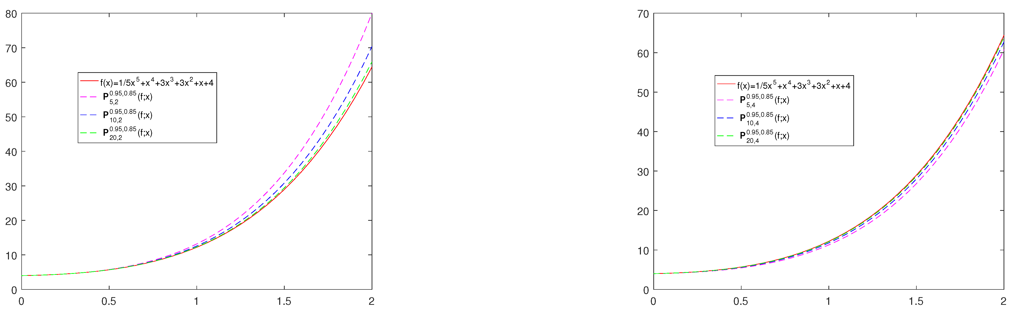
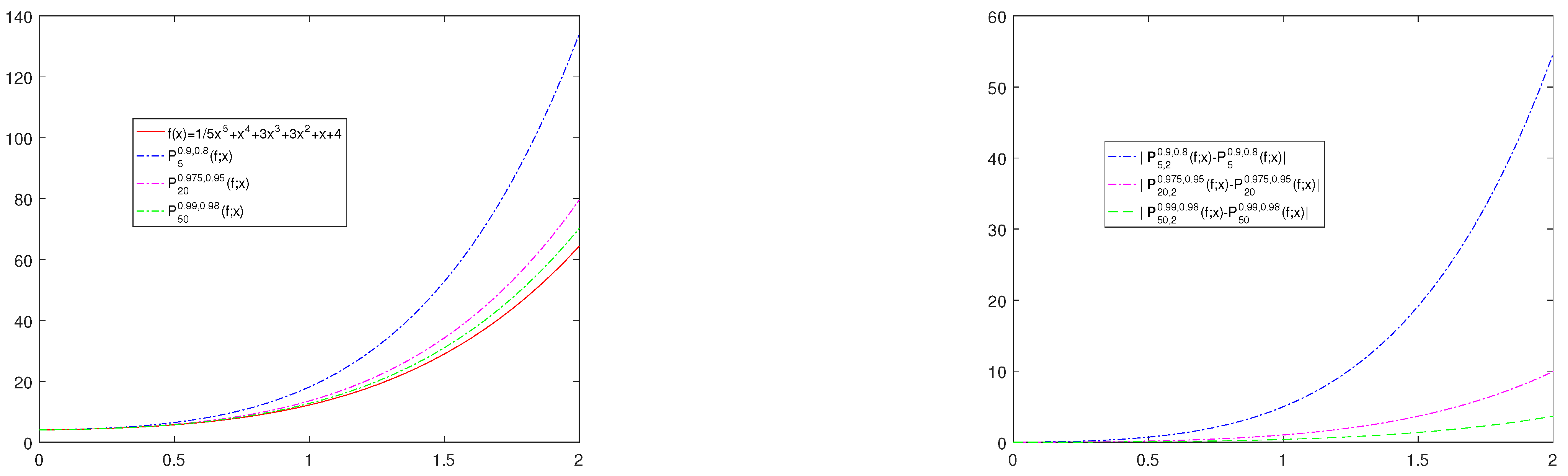
4. Difference of Operators

In this section, we choose $p=p_n$ and $q=q_n$, such that $0<q_n<p_n\le 1$ and $p_n\to 1,q_n\to 1$ and present the quantitative estimates for the differences of $(p,q)$-Post-Widder operator (9) and its modified form (10). Let

$${\phi }_{p,q}(x;t):={\displaystyle \frac{1}{{\Gamma }_{p,q}(n+1)}}{p}^{{\displaystyle \frac{n(n+1)}{2}}}{t}^n{E}_{p,q}(-qt),$$

(31)

then the operators represented by (9) and (10) take the form

$$P_{n,\gamma }^{p,q}(f;x)={\int }_0^{\infty }f\left({\displaystyle \frac{p^{n}xt}{{\left[n\right]}_{p,q}}}\right){\phi }_{p,q}(x;t)d_{p,q}t$$

and

$${\mathbf{P}}_{n,\gamma }^{p,q}(f;x)={\int }_0^{\infty }f\left({\displaystyle \frac{p^{\frac{2n+\gamma +1}{2}}xt}{{\left({[n+1]}_{p,q}\right)}_{\gamma }^{\frac{1}{\gamma }}}}\right){\phi }_{p,q}(x;t)d_{p,q}t.$$

Denote

$$\begin{array}{cc}\hfill b^P=P_n^{p,q}(t;x),& {\mu }_i^P=P_n^{p,q}{(e_1-b^P{e}_0)}^i,\hfill \\ \hfill b^{\mathbf{P}}={\mathbf{P}}_{n,\gamma }^{p,q}(t;x),& {\mu }_i^{\mathbf{P}}={\mathbf{P}}_n^{p,q}{(e_1-b^P{e}_0)}^i,i\in N.\hfill \end{array}$$

It is obvious that ${\mu }_0^P={\mu }_0^{\mathbf{P}}=1$ and ${\mu }_1^P={\mu }_1^{\mathbf{P}}=0$.

Theorem 4.

If $f^{\left(s\right)}\in C_B[0,\infty )$, $s=0,1,2$, then

$$|({\mathbf{P}}_{n,\gamma }^{p,q}-P_n^{p,q})(f;x)|\le {\displaystyle \frac{\parallel f^{″}\parallel }{2}}\alpha \left(x\right)+{\displaystyle \frac{{\omega }_{f^{″}}\left({\delta }_1\right)}{2}}(1+\alpha \left(x\right))+2{\omega }_f\left({\delta }_2\right),$$

(32)

where

$$\begin{array}{cc}\hfill & \alpha \left(x\right)=({\theta }_{n,\gamma }^2\left(x\right)+x^2){\displaystyle \frac{q^{n+1}{[n+1]}_{p,q}}{p^3{\left[n\right]}_{p,q}^2}},\hfill \\ \hfill & {\delta }_1^2=({\displaystyle \frac{{\left({[n+1]}_{p,q}\right)}_4}{p^{10}{\left[n\right]}_{p,q}^4}}-{\displaystyle \frac{4{[n+1]}_{p,q}{\left({[n+1]}_{p,q}\right)}_3}{p^7{\left[n\right]}_{p,q}^4}}+{\displaystyle \frac{6{[n+1]}_{p,q}^2{\left({[n+1]}_{p,q}\right)}_2}{p^5{\left[n\right]}_{p,q}^4}}\hfill \\ \hfill & -{\displaystyle \frac{3{[n+1]}_{p,q}^4}{p^4{\left[n\right]}_{p,q}^4}})({\theta }_{n,\gamma }^4\left(x\right)+x^4),\hfill \\ \hfill & {\delta }_2^2={\displaystyle \frac{{[n+1]}_{p,q}^2}{p^2{\left[n\right]}_{p,q}^2}}{(x-{\theta }_{n,\gamma }\left(x\right))}^2.\hfill \end{array}$$

(33)

Proof. 

We know

$$\begin{array}{cc}\hfill |({\mathbf{P}}_{n,\gamma }^{p,q}-P_n^{p,q})(f;x)|& \le |{\mathbf{P}}_{n,\gamma }^{p,q}(f;x)-f\left(b^{\mathbf{P}}\right)|+|P_n^{p,q}(f;x)-f\left(b^P\right)|\hfill \\ \hfill & +|f\left(b^{\mathbf{P}}\right)-f\left(b^P\right)|:=I_1+I_2+I_3.\hfill \end{array}$$

(34)

Now, using Taylor’s expansion, we have

$$\begin{array}{cc}\hfill f\left(t\right)-f\left(b^{\mathbf{P}}\right)& =f^{\prime }\left(b^{\mathbf{P}}\right)(t-b^{\mathbf{P}})+{\displaystyle \frac{1}{2}}{f}^{″}\left(b^{\mathbf{P}}\right){(t-b^{\mathbf{P}})}^2\hfill \\ \hfill & +{\displaystyle \frac{{(t-b^{\mathbf{P}})}^2}{2}}(f^{″}\left(\xi \right)-f^{″}\left(x\right)),\hfill \end{array}$$

(35)

where $\xi$ lies between t and $b^{\mathbf{P}}$. Applying the operator ${\mathbf{P}}_{n,\gamma }^{p,q}$ on (35) and using Lemma 2,

$$\begin{array}{cc}\hfill I_1& =\left|{\int }_0^{\infty }\left[f\left({\displaystyle \frac{p^{\frac{2n+r+1}{2}}xt}{{\left({[n+1]}_{p,q}\right)}_{\gamma }^{\frac{1}{\gamma }}}}\right)-f\left(b^{\mathbf{P}}\right)\right]{\phi }_{p,q}(x;t)d_{p,q}t\right|\hfill \\ \hfill & =|{\int }_0^{\infty }\{f^{\prime }\left(b^{\mathbf{P}}\right)({\displaystyle \frac{p^{\frac{2n+r+1}{2}}xt}{{\left({[n+1]}_{p,q}\right)}_{\gamma }^{\frac{1}{\gamma }}}}-b^{\mathbf{P}})+{\displaystyle \frac{1}{2}}{f}^{″}\left(b^{\mathbf{P}}\right){({\displaystyle \frac{p^{\frac{2n+r+1}{2}}xt}{{\left({[n+1]}_{p,q}\right)}_{\gamma }^{\frac{1}{\gamma }}}}-b^{\mathbf{P}})}^2\hfill \\ \hfill & +{\displaystyle \frac{{(\frac{p^{\frac{2n+r+1}{2}}xt}{{\left({[n+1]}_{p,q}\right)}_{\gamma }^{\frac{1}{\gamma }}}-b^{\mathbf{P}})}^2}{2}}(f^{″}\left(\xi \right)-f^{″}\left(b^{\mathbf{P}}\right))\}{\phi }_{p,q}(x;t)d_{p,q}t|,\hfill \end{array}$$

here, $\xi$ lies between ${\displaystyle \frac{p^{\frac{2n+r+1}{2}}xt}{{\left({[n+1]}_{p,q}\right)}_{\gamma }^{\frac{1}{\gamma }}}}$ and $b^{\mathbf{P}}$. Using Lemma 2 and

$$|f\left(t\right)-f\left(x\right)|\le \left(1+{\displaystyle \frac{{(t-x)}^2}{h^2}}\right){\omega }_f\left(h\right),$$

so it yields,

$$\begin{array}{cc}\hfill I_1& =|f^{\prime }\left(b^{\mathbf{P}}\right){\mu }_1^{\mathbf{P}}+{\displaystyle \frac{1}{2}}{f}^{″}\left(b^{\mathbf{P}}\right){\mu }_2^{\mathbf{P}}\hfill \\ \hfill & +{\int }_0^{\infty }{\displaystyle \frac{{(\frac{p^{\frac{2n+r+1}{2}}xt}{{\left({[n+1]}_{p,q}\right)}_{\gamma }^{\frac{1}{\gamma }}}-b^{\mathbf{P}})}^2}{2}}(1+{\displaystyle \frac{{(\xi -b^{\mathbf{P}})}^2}{{\delta }_1^2}}){\omega }_{f^{″}}\left({\delta }_1\right){\phi }_{p,q}(x;t)d_{p,q}t|\hfill \\ \hfill & \le {\displaystyle \frac{1}{2}}\parallel f^{″}\parallel {\mu }_2^{\mathbf{P}}+{\displaystyle \frac{1}{2}}{\omega }_{f^{″}}\left({\delta }_1\right)({\mu }_2^{\mathbf{P}}+{\displaystyle \frac{{\mu }_4^{\mathbf{P}}}{{\delta }_1^2}})\hfill \end{array}$$

(36)

and

$$I_3\le \left(1+{\displaystyle \frac{{(b^{\mathbf{P}}-b^P)}^2}{{\delta }_2^2}}\right){\omega }_f\left({\delta }_2\right).$$

(37)

Similary,

$$I_2\le {\displaystyle \frac{1}{2}}\parallel f^{″}\parallel {\mu }_2^P+{\displaystyle \frac{1}{2}}{\omega }_{f^{″}}\left({\delta }_1\right)({\mu }_2^P+{\displaystyle \frac{{\mu }_4^P}{{\delta }_1^2}}).$$

(38)

Then (36), (37) and (38) imply

$$\begin{array}{cc}\hfill |({\mathbf{P}}_{n,\gamma }^{p,q}-P_n^{p,q})(f;x)|& \le {\displaystyle \frac{1}{2}}\parallel f^{″}\parallel ({\mu }_2^P+{\mu }_2^{\mathbf{P}})+{\displaystyle \frac{1}{2}}{\omega }_{f^{″}}\left({\delta }_1\right)({\mu }_2^p+{\mu }_2^{\mathbf{P}}+{\displaystyle \frac{{\mu }_4^P+{\mu }_4^{\mathbf{P}}}{{\delta }_1^2}})\hfill \\ \hfill & +(1+{\displaystyle \frac{{(b^{\mathbf{P}}-b^P)}^2}{{\delta }_2^2}}){\omega }_f\left({\delta }_2\right).\hfill \end{array}$$

Denote $\alpha \left(x\right):={\mu }_2^P+{\mu }_2^{\mathbf{P}}$, ${\delta }_1^2:={\mu }_4^P+{\mu }_4^{\mathbf{P}}$ and ${\delta }_2^2:={(b^{\mathbf{P}}-b^P)}^2$. Thus

$$\begin{array}{cc}\hfill & \alpha \left(x\right)=P_n^{p,q}\left(e_1^2\right)-{\left(P_n^{p,q}\left(e_1\right)\right)}^2+{\mathbf{P}}_{n,\gamma }^{p,q}\left(e_1^2\right)-{\left({\mathbf{P}}_{n,\gamma }^{p,q}\left(e_1\right)\right)}^2\hfill \\ \hfill & ={\displaystyle \frac{{\left({[n+1]}_{p,q}\right)}_2}{p^3{\left[n\right]}_{p,q}^2}}{x}^2-{\displaystyle \frac{{[n+1]}_{p,q}^2}{p^2{\left[n\right]}_{p,q}^2}}{x}^2+{\displaystyle \frac{{\left({[n+1]}_{p,q}\right)}_2}{p^3{\left[n\right]}_{p,q}^2}}{\theta }_{n,\gamma }^2\left(x\right)-{\displaystyle \frac{{[n+1]}_{p,q}^2}{p^2{\left[n\right]}_{p,q}^2}}{\theta }_{n,\gamma }^2\left(x\right)\hfill \\ \hfill & =({\theta }_{n,\gamma }^2\left(x\right)+x^2){\displaystyle \frac{q^{n+1}{[n+1]}_{p,q}}{p^3{\left[n\right]}_{p,q}^2}},\hfill \end{array}$$

$$\begin{array}{cc}\hfill {\delta }_1^2& =P_n^{p,q}{(e_1-b^P{e}_0)}^4+{\mathbf{P}}_{n,\gamma }^{p,q}{(e_1-b^P{e}_0)}^4\hfill \\ \hfill & =P_n^{p,q}\left(e_1^4\right)-4P_n^{p,q}\left(e_1\right)P_n^{p,q}\left(e_1^3\right)+6{\left(P_n^{p,q}\left(e_1\right)\right)}^2{P}_n^{p,q}\left(e_1^2\right)-3{\left(P_n^{p,q}\left(e_1\right)\right)}^4\hfill \\ \hfill & +{\mathbf{P}}_n^{p,q}\left(e_1^4\right)-4{\mathbf{P}}_n^{p,q}\left(e_1\right){\mathbf{P}}_n^{p,q}\left(e_1^3\right)+6{\left({\mathbf{P}}_n^{p,q}\left(e_1\right)\right)}^2{\mathbf{P}}_n^{p,q}\left(e_1^2\right)-3{\left({\mathbf{P}}_n^{p,q}\left(e_1\right)\right)}^4\hfill \\ \hfill & =({\displaystyle \frac{{\left({[n+1]}_{p,q}\right)}_4}{p^{10}{\left[n\right]}_{p,q}^4}}-{\displaystyle \frac{4{[n+1]}_{p,q}{\left({[n+1]}_{p,q}\right)}_3}{p^7{\left[n\right]}_{p,q}^4}}+{\displaystyle \frac{6{[n+1]}_{p,q}^2{\left({[n+1]}_{p,q}\right)}_2}{p^5{\left[n\right]}_{p,q}^4}}\hfill \\ \hfill & -{\displaystyle \frac{3{[n+1]}_{p,q}^4}{p^4{\left[n\right]}_{p,q}^4}})({\theta }_{n,\gamma }^4\left(x\right)+x^4)\hfill \end{array}$$

and

$${\delta }_2^2={\displaystyle \frac{{[n+1]}_{p,q}^2}{p^2{\left[n\right]}_{p,q}^2}}{(x-{\theta }_{n,\gamma }\left(x\right))}^2.$$

Hence, (32) is verified, and the proof of Theorem 4 is complete. □

Theorem 5.

Let $f^{\left(s\right)}\in C_B[0,\infty )$, $s=0,1,2,3,4$. Then

$$|({\mathbf{P}}_{n,\gamma }^{p,q}-P_n^{p,q})(f;x)|\le {\displaystyle \frac{\parallel f^{″}\parallel }{2}}\alpha \left(x\right)+{\displaystyle \frac{\parallel f^{‴}\parallel }{3!}}\beta \left(x\right)+{\displaystyle \frac{\parallel f^{\left(4\right)}\parallel }{4!}}{\delta }_1^2+2{\omega }_f\left({\delta }_2\right),$$

(39)

where

$$\begin{array}{cc}\hfill \beta \left(x\right)& =\left({\displaystyle \frac{{\left({[n+1]}_{p,q}\right)}_3}{p^6{\left[n\right]}_{p,q}^3}}-{\displaystyle \frac{3{[n+1]}_{p,q}{\left({[n+1]}_{p,q}\right)}_2}{p^4{\left[n\right]}_{p,q}^3}}+{\displaystyle \frac{2{[n+1]}_{p,q}^3}{p^3{\left[n\right]}_{p,q}^3}}\right)({\theta }_{n,\gamma }^3\left(x\right)+x^3),\hfill \end{array}$$

$\alpha \left(x\right)$, ${\delta }_1$ and ${\delta }_2$ are given by (33).

Proof. 

Using Taylor’s expansion of the fourth order, we have

$$\begin{array}{cc}\hfill f\left(t\right)-f\left(b^{\mathbf{P}}\right)& =f^{\prime }\left(b^{\mathbf{P}}\right)(t-b^{\mathbf{P}})+{\displaystyle \frac{1}{2}}{f}^{″}\left(b^{\mathbf{P}}\right){(t-b^{\mathbf{P}})}^2\hfill \\ \hfill & +{\displaystyle \frac{f^{‴}\left(b^{\mathbf{P}}\right)}{3!}}{(t-b^{\mathbf{P}})}^3+{\displaystyle \frac{f^{\left(4\right)}\left(\xi \right)}{4!}}{(t-b^{\mathbf{P}})}^4,\hfill \end{array}$$

(40)

where $\xi$ lies between t and $b^{\mathbf{P}}$. In view of (34) and (40), we obtain

$$\begin{array}{cc}\hfill I_1& =|f^{\prime }\left(b^{\mathbf{P}}\right){\mu }_1^{\mathbf{P}}+{\displaystyle \frac{1}{2}}{f}^{″}\left(b^{\mathbf{P}}\right){\mu }_2^{\mathbf{P}}+{\displaystyle \frac{1}{3!}}{f}^{‴}\left(b^{\mathbf{P}}\right){\mu }_3^{\mathbf{P}}\hfill \\ \hfill & +{\displaystyle \frac{1}{4!}}{\int }_0^{\infty }{f}^{\left(4\right)}\left(\xi \right){({\displaystyle \frac{p^{\frac{2n+\gamma +1}{2}}xt}{{\left({[n+1]}_{p,q}\right)}_{\gamma }^{\frac{1}{\gamma }}}}-b^{\mathbf{P}})}^4{\phi }_{p,q}(x;t)d_{p,q}t|\hfill \\ \hfill & \le {\displaystyle \frac{1}{2}}\parallel f^{″}\parallel {\mu }_2^{\mathbf{P}}+{\displaystyle \frac{\parallel f^{‴}\parallel }{3!}}{\mu }_3^{\mathbf{P}}+{\displaystyle \frac{\parallel f^{\left(4\right)}\parallel }{4!}}{\mu }_4^{\mathbf{P}}.\hfill \end{array}$$

Using a similar method, we have

$$I_2\le {\displaystyle \frac{1}{2}}\parallel f^{″}\parallel {\mu }_2^P+{\displaystyle \frac{\parallel f^{‴}\parallel }{3!}}{\mu }_3^P+{\displaystyle \frac{\parallel f^{\left(4\right)}\parallel }{4!}}{\mu }_4^P.$$

With the help of (37), we obtain

$$\begin{array}{cc}\hfill |({\mathbf{P}}_{n,\gamma }^{p,q}-P_n^{p,q})(f;x)|& \le {\displaystyle \frac{1}{2}}\parallel f^{″}\parallel ({\mu }_2^P+{\mu }_2^{\mathbf{P}})+{\displaystyle \frac{1}{3!}}\parallel f^{‴}\parallel ({\mu }_3^P+{\mu }_3^{\mathbf{P}})\hfill \\ \hfill & +{\displaystyle \frac{1}{4!}}\parallel f^{\left(4\right)}\parallel ({\mu }_4^P+{\mu }_4^{\mathbf{P}})+(1+{\displaystyle \frac{{(b^{\mathbf{P}}-b^P)}^2}{{\delta }_2^2}}){\omega }_f\left({\delta }_2\right).\hfill \end{array}$$

Let $\alpha \left(x\right):={\mu }_2^P+{\mu }_2^{\mathbf{P}}$, $\beta \left(x\right):={\mu }_3^P+{\mu }_3^{\mathbf{P}}$, ${\delta }_1^2:={\mu }_4^P+{\mu }_4^{\mathbf{P}}$ and ${\delta }_2^2:={(b^{\mathbf{P}}-b^P)}^2$. By simple computation, we have

$$\begin{array}{cc}\hfill \beta \left(x\right)& =P_n^{p,q}{(e_1-b^P{e}_0)}^3+{\mathbf{P}}_{n,\gamma }^{p,q}{(e_1-b^P{e}_0)}^3\hfill \\ \hfill & =P_n^{p,q}\left(e_1^3\right)-3P_n^{p,q}\left(e_1\right)P_n^{p,q}\left(e_1^2\right)+2{\left(P_n^{p,q}\left(e_1\right)\right)}^3+{\mathbf{P}}_{n,\gamma }^{p,q}\left(e_1^3\right)\hfill \\ \hfill & -3{\mathbf{P}}_{n,\gamma }^{p,q}\left(e_1\right){\mathbf{P}}_{n,\gamma }^{p,q}\left(e_1^2\right)+2{\left({\mathbf{P}}_{n,\gamma }^{p,q}\left(e_1\right)\right)}^3\hfill \\ \hfill & =\left({\displaystyle \frac{{\left({[n+1]}_{p,q}\right)}_3}{p^6{\left[n\right]}_{p,q}^3}}-{\displaystyle \frac{3{[n+1]}_{p,q}{\left({[n+1]}_{p,q}\right)}_2}{p^4{\left[n\right]}^{p,q}}}+{\displaystyle \frac{2{[n+1]}_{p,q}^3}{p^3{\left[n\right]}_{p,q}^3}}\right)({\theta }_{n,\gamma }^3\left(x\right)+x^3),\hfill \end{array}$$

The estimates of $\alpha \left(x\right)$, ${\delta }_1$ and ${\delta }_2$ can be obtained using Theorem 4. This completes the proof. □

Now, we prove the differences betweeen operators $P_n^{p,q}$ and ${\mathbf{P}}_{n,\gamma }^{p,q}$ in quantitative form using the weighted modulus of smoothness (20).

Theorem 6.

Let $f\in C_2[0,\infty )$ with $f^{″}\in C_{B_2}[0,\infty )$. Then

$$\begin{array}{cc}\hfill |({\mathbf{P}}_{n,\gamma }^{p,q}-P_n^{p,q})(f;x)|& \le {\displaystyle \frac{1}{2}}{\parallel f^{″}\parallel }_2\zeta \left(x\right)+8\Omega (f^{″};{\varsigma }_1)(1+\zeta \left(x\right))\hfill \\ \hfill & +16\Omega (f^{″};{\varsigma }_2)(1+\varphi \left(x\right)),\hfill \end{array}$$

where

$$\begin{array}{cc}\hfill & \zeta \left(x\right)={\displaystyle \frac{{[n+1]}_{p,q}^2{q}^{n+1}}{p^3{\left[n\right]}_{p,q}^2}}\left({\theta }_{n,\gamma }^2\left(x\right)+x^2+{\displaystyle \frac{{[n+1]}_{p,q}^2}{p^2{\left[n\right]}_{p,q}^2}}({\theta }_{n,\gamma }^4\left(x\right)+x^4)\right),\hfill \\ \hfill & {\varsigma }_1^4=({\displaystyle \frac{{\left([n+1]\right)}_6}{p^{21}{\left[n\right]}_{p,q}^6}}-{\displaystyle \frac{6{[n+1]}_{p,q}{\left({[n+1]}_{p,q}\right)}_5}{p^{16}{\left[n\right]}_{p,q}^6}}+{\displaystyle \frac{15{[n+1]}_{p,q}^2{\left({[n+1]}_{p,q}\right)}_4}{p^{12}{\left[n\right]}_{p,q}^6}}\hfill \\ \hfill & -{\displaystyle \frac{20{[n+1]}_{p,q}^3{\left({[n+1]}_{p,q}\right)}_3}{p^9{\left[n\right]}_{p,q}^6}}+{\displaystyle \frac{15{[n+1]}_{p,q}^4{\left({[n+1]}_{p,q}\right)}_2}{p^7{\left[n\right]}_{p,q}^6}}\hfill \\ \hfill & -{\displaystyle \frac{5{[n+1]}_{p,q}^6}{p^6{\left[n\right]}_{p,q}^6}})\left({\theta }_{n,\gamma }^6\left(x\right)+x^6+{\displaystyle \frac{p^{-2}{[n+1]}_{p,q}^2}{{\left[n\right]}_{p,q}^2}}({\theta }_{n,\gamma }^8\left(x\right)+x^8)\right),\hfill \\ \hfill & {\varsigma }_2^4={\displaystyle \frac{{[n+1]}_{p,q}^4}{p^4{\left[n\right]}_{p,q}^4}}(1+{\displaystyle \frac{{[n+1]}_{p,q}^2}{p^2{\left[n\right]}_{p,q}^2}}{x}^2){({\theta }_{n,\gamma }\left(x\right)-x)}^4,\hfill \\ \hfill & \varphi \left(x\right)=1+{\displaystyle \frac{{[n+1]}_{p,q}^2}{p^2{\left[n\right]}_{p,q}^2}}{x}^2.\hfill \end{array}$$

Proof. 

It was shown in [27] that

$$|f\left(y\right)-f\left(x\right)|\le 16(1+x^2)\Omega (f;\delta )(1+{\displaystyle \frac{{(y-x)}^4}{{\delta }^4}}).$$

(41)

Using (34), (35) and (41), we can write

$$\begin{array}{cc}\hfill & I_1\le f^{\prime }\left(b^{\mathbf{P}}\right){\mu }_1^{\mathbf{P}}+{\displaystyle \frac{1}{2}}{f}^{″}\left(b^{\mathbf{P}}\right){\mu }_2^{\mathbf{P}}+{\displaystyle \frac{1}{2}}{\int }_0^{\infty }16(1+{\left(b^{\mathbf{P}}\right)}^2)\Omega (f^{″};{\delta }_1^{*})\times \hfill \\ \hfill & \times {({\displaystyle \frac{p^{\frac{2n+\gamma +1}{2}}xt}{{\left({[n+1]}_{p,q}\right)}_{\gamma }^{\frac{1}{\gamma }}}}-b^{\mathbf{P}})}^2(1+{\displaystyle \frac{{(\xi -b^{\mathbf{P}})}^4}{{\delta }_1^{*4}}}){\phi }_{p,q}(x;t)d_{p,q}t|\hfill \\ \hfill & \le {\displaystyle \frac{1}{2}}\left|{\displaystyle \frac{f^{″}\left(b^{\mathbf{P}}\right)}{1+{\left(b^{\mathbf{P}}\right)}^2}}\right|(1+{\left(b^{\mathbf{P}}\right)}^2){\mu }_2^{\mathbf{P}}+8(1+{\left(b^{\mathbf{P}}\right)}^2)({\mu }_2^{\mathbf{P}}+{\displaystyle \frac{{\mu }_6^{\mathbf{P}}}{{\delta }_1^{*4}}})\Omega (f^{″},{\delta }_1^{*})\hfill \\ \hfill & \le {\displaystyle \frac{1}{2}}{\parallel f^{″}\parallel }_2\left[(1+{\left(b^{\mathbf{P}}\right)}^2){\mu }_2^{\mathbf{P}}\right]+8\Omega (f^{″},{\delta }_1^{*})\left((1+{\left(b^{\mathbf{P}}\right)}^2){\mu }_2^{\mathbf{P}}+{\displaystyle \frac{(1+{\left(b^{\mathbf{P}}\right)}^2){\mu }_6^{\mathbf{P}}}{{\delta }_1^{*4}}}\right),\hfill \end{array}$$

and

$$\begin{array}{cc}\hfill I_3& =|f\left(b^{\mathbf{P}}\right)-f\left(b^P\right)|\le 16(1+{\left(b^P\right)}^2)\Omega (f^{″},{\varsigma }_2)(1+{\displaystyle \frac{{(b^{\mathbf{P}}-b^P)}^4}{{\varsigma }_2^4}})\hfill \\ \hfill & =16\Omega (f^{″},{\varsigma }_2)\left(1+{\left(b^P\right)}^2+{\displaystyle \frac{{(b^{\mathbf{P}}-b^P)}^4[1+{\left(b^P\right)}^2]}{{\varsigma }_2^4}}\right).\hfill \end{array}$$

Similar to the proof of $I_1$, we have

$$\begin{array}{cc}\hfill I_2& \le {\displaystyle \frac{1}{2}}{\parallel f^{″}\parallel }_2\left((1+{\left(b^P\right)}^2){\mu }_2^P\right)\hfill \\ \hfill & +8\Omega (f^{″},{\varsigma }_1)\left((1+{\left(b^P\right)}^2){\mu }_2^p+{\displaystyle \frac{(1+{\left(b^P\right)}^2){\mu }_6^p}{{\varsigma }_1^4}}\right).\hfill \end{array}$$

Thus,

$$\begin{array}{cc}\hfill \left|\right({\mathbf{P}}_{n,\gamma }^{p,q}& -P_n^{p,q}\left)(f;x)\right|\le {\displaystyle \frac{1}{2}}{\parallel f^{″}\parallel }_2\left((1+{\left(b^{\mathbf{P}}\right)}^2){\mu }_2^{\mathbf{P}}+(1+{\left(b^P\right)}^2){\mu }_2^P\right)\hfill \\ \hfill & +8\Omega (f^{″},{\varsigma }_1)((1+{\left(b^{\mathbf{P}}\right)}^2){\mu }_2^{\mathbf{P}}+(1+{\left(b^P\right)}^2){\mu }_2^P\hfill \\ \hfill & +{\displaystyle \frac{(1+{\left(b^{\mathbf{P}}\right)}^2){\mu }_6^{\mathbf{P}}+(1+{\left(b^P\right)}^2){\mu }_6^P}{{\varsigma }_1^4}})\hfill \\ \hfill & +16\Omega (f^{″},{\varsigma }_2)\left(1+{\left(b^P\right)}^2+{\displaystyle \frac{{(b^{\mathbf{P}}-b^P)}^4[1+{\left(b^P\right)}^2]}{{\varsigma }_2^4}}\right)\hfill \\ \hfill & ={\displaystyle \frac{1}{2}}{\parallel f^{″}\parallel }_2\zeta \left(x\right)+8\Omega (f^{″};{\varsigma }_1)(1+\zeta \left(x\right))+16\Omega (f^{″};{\varsigma }_2)(1+\varphi \left(x\right)),\hfill \end{array}$$

(42)

where

$$\begin{array}{cc}\hfill \zeta \left(x\right)& :=(1+{\left(b^{\mathbf{P}}\right)}^2){\mu }_2^{\mathbf{P}}+(1+{\left(b^P\right)}^2){\mu }_2^P,\hfill \\ \hfill {\varsigma }_1^4& :=(1+{\left(b^{\mathbf{P}}\right)}^2){\mu }_6^{\mathbf{P}}+(1+{\left(b^P\right)}^2){\mu }_6^P,\hfill \\ \hfill {\varsigma }_2^4& :=(1+{\left(b^P\right)}^2){(b^P-b^{\mathbf{P}})}^4,\varphi \left(x\right):=1+{\left(b^P\right)}^2.\hfill \end{array}$$

By a simple calculation, we immediately derive

$$\begin{array}{cc}\hfill \zeta \left(x\right)& =\left(1+({\mathbf{P}}_{n,\gamma }^{p,q}{\left(e_1\right)}^2\right)\left({\mathbf{P}}_{n,\gamma }^{p,q}\left(e_1^2\right)-{\left({\mathbf{P}}_{n,\gamma }^{p,q}\left(e_1\right)\right)}^2\right)\hfill \\ \hfill & +\left(1+{\left(P_n^{p,q}\left(e_1\right)\right)}^2\right)\left(P_n^{p,q}\left(e_1^2\right)-{\left(P_n^{p,q}\left(e_1\right)\right)}^2\right)\hfill \\ \hfill & ={\displaystyle \frac{{[n+1]}_{p,q}^2{q}^{n+1}}{p^3{\left[n\right]}_{p,q}^2}}\left({\theta }_{n,\gamma }^2\left(x\right)+x^2+{\displaystyle \frac{{[n+1]}_{p,q}^2}{p^2{\left[n\right]}_{p,q}^2}}({\theta }_{n,\gamma }^4\left(x\right)+x^4)\right).\hfill \end{array}$$

Also,

$$\begin{array}{cc}\hfill {\varsigma }_2^4& ={\displaystyle \frac{{[n+1]}_{p,q}^4}{p^4{\left[n\right]}_{p,q}^4}}(1+{\displaystyle \frac{{[n+1]}_{p,q}^2}{p^2{\left[n\right]}_{p,q}^2}}{x}^2){({\theta }_{n,\gamma }\left(x\right)-x)}^4\hfill \end{array}$$

and

$$\varphi \left(x\right)=1+{\displaystyle \frac{{[n+1]}_{p,q}^2}{p^2{\left[n\right]}_{p,q}^2}}{x}^2.$$

Using the definition of ${\mu }_i^P$ and Lemma 1, we obtain

$$\begin{array}{cc}\hfill & {\mu }_6^P=P_n^{p,q}\left(e_1^6\right)-6b^P{P}_n^{p,q}\left(e_1^5\right)+15{\left(b^P\right)}^2{P}_n^{p,q}\left(e_1^4\right)-20{\left(b^P\right)}^3{P}_n^{p,q}\left(e_1^3\right)\hfill \\ \hfill & +15{\left(b^P\right)}^4{P}_n^{p,q}\left(e_1^2\right)-6{\left(b^P\right)}^5{P}_n^{p,q}\left(e_1\right)+{\left(b^P\right)}^6\hfill \\ \hfill & =({\displaystyle \frac{{\left([n+1]\right)}_6}{p^{21}{\left[n\right]}_{p,q}^6}}-{\displaystyle \frac{6{[n+1]}_{p,q}{\left({[n+1]}_{p,q}\right)}_5}{p^{16}{\left[n\right]}_{p,q}^6}}+{\displaystyle \frac{15{[n+1]}_{p,q}^2{\left({[n+1]}_{p,q}\right)}_4}{p^{12}{\left[n\right]}_{p,q}^6}}\hfill \\ \hfill & -{\displaystyle \frac{20{[n+1]}_{p,q}^3{\left({[n+1]}_{p,q}\right)}_3}{p^9{\left[n\right]}_{p,q}^6}}+{\displaystyle \frac{15{[n+1]}_{p,q}^4{\left({[n+1]}_{p,q}\right)}_2}{p^7{\left[n\right]}_{p,q}^6}}-{\displaystyle \frac{5{[n+1]}_{p,q}^6}{p^6{\left[n\right]}_{p,q}^6}})x^6.\hfill \end{array}$$

(43)

Proceeding similarly, we obtain

$$\begin{array}{cc}\hfill {\mu }_6^{\mathbf{P}}& =({\displaystyle \frac{{\left([n+1]\right)}_6}{p^{21}{\left[n\right]}_{p,q}^6}}-{\displaystyle \frac{6{[n+1]}_{p,q}{\left({[n+1]}_{p,q}\right)}_5}{p^{16}{\left[n\right]}_{p,q}^6}}+{\displaystyle \frac{15{[n+1]}_{p,q}^2{\left({[n+1]}_{p,q}\right)}_4}{p^{12}{\left[n\right]}_{p,q}^6}}\hfill \\ \hfill & -{\displaystyle \frac{20{[n+1]}_{p,q}^3{\left({[n+1]}_{p,q}\right)}_3}{p^9{\left[n\right]}_{p,q}^6}}+{\displaystyle \frac{15{[n+1]}_{p,q}^4{\left({[n+1]}_{p,q}\right)}_2}{p^7{\left[n\right]}_{p,q}^6}}\hfill \\ \hfill & -{\displaystyle \frac{5{[n+1]}_{p,q}^6}{p^6{\left[n\right]}_{p,q}^6}}){\theta }_{n,\gamma }^6\left(x\right).\hfill \end{array}$$

(44)

Considering (43) and (44), we obtain the value of ${\varsigma }_1^4$. Thus, the proof is completed. □

5. Graphical Analysis

Now, let us return our attention to the test function $f\left(x\right)={\displaystyle \frac{1}{5}}{x}^5+x^4+3x^3+3x^2+x+4$ to verify our claim numerically. Firstly, we present the convergence of operators ${\mathbf{P}}_{n,\gamma }^{p,q}$ for different values of $\gamma$. From Figure 1, one can see the convergence of operators ${\mathbf{P}}_{15,\gamma }^{0.95,0.85}$ (Figure 1a) and ${\mathbf{P}}_{15,\gamma }^{1,0.89}$ (Figure 1b) for $\gamma =1,2,3,4,5$. Moreover, Figure 1c,d shows the corresponding plots for the magnitude of differences. From the above graphs, we conclude that the estimation error of the operators ${\mathbf{P}}_{n,\gamma }^{p,q}$ decreases from $\gamma =1$ to $\gamma =3$, after which it starts to increase. Therefore, the best approximation by the operators ${\mathbf{P}}_{n,\gamma }^{p,q}$ happens at $\gamma =3$.

Next, in Figure 2, one can see the convergence of operator ${\mathbf{P}}_{n,\gamma }^{p,q}$ for fixed values for parameters p, q, and $\gamma$ and for different values of n. We observe that the introduced operator ${\mathbf{P}}_{n,\gamma }^{p,q}$ converges better to the test function as parameter n increases. In Figure 3, we show the convergence of operators defined in (10) to the function $f\left(x\right)$ for $p=p_n=1-{\displaystyle \frac{1}{2n}}$, $q=q_n=1-{\displaystyle \frac{1}{n}}$, $\gamma =2$ (Figure 3a), $\gamma =3$ (Figure 3b) and $n=5,20,50$. It is obvious from Figure 2 and Figure 3 that the larger the n value, the better the approximation.

Finally, from the Figure 4a, it can be observed that as $p_n$ and $q_n$ approach 1, provided $0<q_n<p_n\le 1$, the operator $P_n^{p_n,q_n}(f;x)$ converges towards the function. Observe that Figure 3a,b presents a better result than Figure 4a. The operator ${\mathbf{P}}_{n,\gamma }^{p,q}$ is slightly better than the $(p,q)$-Post-Widder operator $P_n^{p,q}$. Also, Figure 4b shows the plot of the magnitude of differences $|{\mathbf{P}}_{n,2}^{p_n,q_n}(f;x)-P_n^{p_n,q_n}(f;x)|$ for $n=5,20,50$, $p_n=1-{\displaystyle \frac{1}{2n}}$ and $q_n=1-{\displaystyle \frac{1}{n}}$. It is worthwhile mentioning that from the numerical results, it ca be seen that for a larger n value, both the operator ${\mathbf{P}}_{n,\gamma }^{p,q}$ and operator $P_n^{p,q}$ perform almost the same as n grows larger.

6. Conclusions

In recent years, several researchers have studied problems concerning the modified classical linear positive operators fixing 1 and $x^{\gamma }$ for a given $\gamma \in \mathbb{N}$. The aim of this paper is to construct a new $(p,q)$-Post-Widder operator ${\mathbf{P}}_{n,\gamma }^{p,q}$ preserving $x^{\gamma }$. Here, we consider new $(p,q)$-Post-Widder operators $P_n^{p,q}$ and their modified form ${\mathbf{P}}_{n,\gamma }^{p,q}$.we obtain the convergence properties of the operator ${\mathbf{P}}_{n,\gamma }^{p,q}$ in terms of the modulus of continuity and the weighted modulus of continuity. Finally, we obtain an estimation of the difference between operators $P_n^{p,q}$ and ${\mathbf{P}}_{n,\gamma }^{p,q}$. According to the numerical and graphical analyses, we deduce that a better approximation is obtained only when the test function $x^3$ is preserved.As the $\gamma$ increases, we cannot obtain a better approximation. Furthermore, operator ${\mathbf{P}}_{n,\gamma }^{p,q}$, in some sense, provides a better estimate than the operator $P_n^{p,q}$. Inspired by [28,29,30,31,32], in future work, we plan to investigate these research topics.

References

1. Ditzian, Z.; Totik, V. Moduli of Smoothness; Springer: New York, NY, USA, 1987. [Google Scholar]
2. Rempulska, L.; Rempulska, M. The Voronovskaya-type theorems for Post-Widder and Stancu operators. Int. J. Pure Appl. Math. 2007, 38, 467. [Google Scholar]
3. King, J. Positive linear operators which preserve x2. Acta Math. Hungar. 2003, 99, 203–208. [Google Scholar]
4. Aldaz, J.M.; Kounchev, O.; Render, H. Shape preserving properties of generalized Bernstein operators on extended Chebyshev spaces. Numer. Math. 2009, 114, 1–25. [Google Scholar]
5. Rempulska, L.; Skorupka, M. On Approximation by Post-Widder and Stancu Operators Preserving x2. Kyungpook Math. J. 2009, 49, 57–65. [Google Scholar] [CrossRef]
6. May, C. Saturation and inverse theorems for combinations of a class of exponential-type operators. Can. J. Math. 1976, 28, 1224–1250. [Google Scholar] [CrossRef]
7. Siddiqui, M.A.; Agrawal, R.R. A Voronovskaya Type Theorem on Modified Post-Widder Operators Preserving x2. Kyungpook Math. J. 2011, 51, 87–91. [Google Scholar]
8. Gupta, V.; Agrawal, D. Convergence by modified Post-Widder operators. Rev. Real Acad. Cienc. Exactas Físicas Nat. Ser. A Matemáticas 2019, 113, 1475–1486. [Google Scholar]
9. Gupta, V.; Tachev, G. Some results on Post-Widder operators preserving test function xr. Kragujev. J. Math. 2022, 46, 149–165. [Google Scholar]
10. Srivastav, R.K.; Deshwal, S. Convergence: New Post-Widder operators. Int. J. Math. Trends Technol.-IJMTT 2021, 67, 43–52. [Google Scholar]
11. Abel, U.; Acu, A.M.; Heilmann, M.; Raşa, I. Positive linear operators preserving certain monomials on [0,). Dolomites Res. Notes Approx. 2023, 16, 1–9. [Google Scholar]
12. Jackson, F.H. On q-definite integrals. Quart. J. Pure Appl. Math. 1910, 41, 193–203. [Google Scholar]
13. De Sole, A.; Kac, V. On integral representations of q-gamma and q-beta functions. Atti Accad. Naz. Lincei Cl. Sci. Fis. Mat. Nat. IX Ser. Rend. Lincei Mat. Appl. 2005, 16, 11–29. [Google Scholar]
14. Ünal, Z.; Özarslan, M.A.; Duman, O. Approximation properties of real and complex post-widder operators based on q-integers. Miskolc Math. Notes 2012, 13, 581–603. [Google Scholar] [CrossRef]
15. Mursaleen, M.; Ansari, K.J.; Khan, A. On (p, q)-analogue of bernstein operators. Appl. Math. Comput. 2015, 266, 874–882. [Google Scholar] [CrossRef]
16. Mursaleen, M.; Alotaibi, A.; Ansari, K.J. On a Kantorovich Variant of (p, q)-Szász-Mirakjan Operators. J. Funct. Space 2016, 2016, 035253. [Google Scholar] [CrossRef]
17. Mursaleen, M.; Ansari, K.J.; Khan, A. Some approximation results by (p, q)-analogue of Bernstein-Stancu operators. Appl. Math. Comput. 2015, 264, 392–402. [Google Scholar] [CrossRef]
18. Malik, N.; Gupta, V. Approximation by (p, q)-Baskakov-Beta operators. Appl. Math. Comput. 2017, 293, 49–56. [Google Scholar] [CrossRef]
19. Mohiuddine, S.A.; Alotaibi, A. Durrmeyer type (p, q)-Baskakov operators preserving linear functions. J. Math. Inequal. 2018, 12, 961–973. [Google Scholar] [CrossRef]
20. Kantar, U.D.; Yuksel, I. Investigating (p, q)-hybrid Durrmeyer–type operators in terms of their approximation properties. Gazi Univ. J. Sci. Part A Eng. Innov. 2022, 2022, 1–11. [Google Scholar]
21. Gupta, V.; Rassias, T.M.; Agrawal, P.; Acu, A.M. Recent Advances in Constructive Approximation Theory; Springer: New York, NY, USA, 2018. [Google Scholar]
22. Aral, A.; Gupta, V. Applications of (p,q)-Gamma functions to Szász-Durrmeyer operators. Publ. Inst. Math. 2017, 102, 211–220. [Google Scholar] [CrossRef]
23. Mishra, V.N.; Pandey, S.; Mishra, L.N. On King Type Modification of (p,q)-Baskakov Operators which preserves x2. arXiv 2016, arXiv:1603.05510. [Google Scholar]
24. Cheng, W.T.; Zhang, W.H.; Cai, Q.B. (p,q)-gamma operators which preserve x2. J. Inequal. Appl. 2019, 2019, 108. [Google Scholar] [CrossRef]
25. Ispir, N. On modified Baskakov operators on weighted spaces. Turk. J. Math. 2001, 25, 355–365. [Google Scholar]
26. DeVore, R. Constructive Approximation; Springer: Berlin, Germany, 1993. [Google Scholar]
27. Aral, A.; Inoan, D.; Raşa, I. On differences of linear positive operators. Anal. Math. Phys. 2019, 9, 1227–1239. [Google Scholar] [CrossRef]
28. Li, F.; Wang, J. Analysis of an HIV infection model with logistic target-cell growth and cell-to-cell transmission. Chaos Solitons Fractals 2015, 81, 136–145. [Google Scholar] [CrossRef]
29. Li, F.; Yu, P.; Tian, Y.; Liu, Y. Center and isochronous center conditions for switching systems associated with elementary singular points. Commun. Nonlinear Sci. 2015, 28, 81–97. [Google Scholar] [CrossRef]
30. Li, F.; Liu, Y.; Liu, Y.; Yu, P. Bi-center problem and bifurcation of limit cycles from nilpotent singular points in Z2-equivariant cubic vector fields. J. Differ. Equations 2018, 265, 4965–4992. [Google Scholar] [CrossRef]
31. Li, F.; Yu, P.; Liu, Y.; Liu, Y. Centers and isochronous centers of a class of quasi-analytic switching systems. Sci. China Math. 2018, 61, 1201–1218. [Google Scholar] [CrossRef]
32. Chen, T.; Li, F.; Yu, P. Nilpotent center conditions in cubic switching polynomial Liénard systems by higher-order analysis. J. Differ. Equations 2024, 379, 258–289. [Google Scholar] [CrossRef]
Figure 1. The convergence and error of operators P 15 , γ 0.95 , 0.85 ( f ; x ) and P 15 , γ 1 , 0.89 ( f ; x ) to f ( x ) for γ = 1 , 2 , 3 , 4 , 5 . (a,b) show the convergence of P 15 , γ 0.95 , 0.85 ( f ; x ) and P 15 , γ 1 , 0.89 ( f ; x ) to f ( x ) for γ = 1 , 2 , 3 , 4 , 5 . (c,d) show the corresponding approximation errors | P 15 , γ 0.95 , 0.85 ( f ; x ) f ( x ) | and | P 15 , γ 1 , 0.89 ( f ; x ) f ( x ) | .
Symmetry 17 00553 g001
Figure 2. The convergence of operators P n , 2 0.95 , 0.85 ( f ; x ) and P n , 4 0.95 , 0.85 ( f ; x ) to f ( x ) for n = 5 , 10 , 20 .
Symmetry 17 00553 g002
Figure 3. The convergence of operators P n , 2 p n , q n ( f ; x ) and P n , 3 p n , q n ( f ; x ) to f ( x ) for n = 5 , 20 , 50 , p n = 1 1 2 n and q n = 1 1 n .
Symmetry 17 00553 g003
Figure 4. The convergence of operators P n p n , q n ( f ; x ) to f ( x ) and the plot of the quantities | P n , 2 p n , q n ( f ; x ) P n p n , q n ( f ; x ) | for n = 5 , 20 , 50 , p n = 1 1 2 n and q n = 1 1 n .
Symmetry 17 00553 g004