Parameter Estimation of PV Solar Cells and Modules Using Deep Learning-Based White Shark Optimizer Algorithm

Abstract

Photovoltaic systems are affected by light intensity, temperature, and radiation angle, which influence their efficiency. Accurate estimation of PV module parameters is essential for improving performance. This paper presents an improved optimization technique based on the White Shark Optimizer (WSO) algorithm to optimize key characteristics of the PV module, including current, voltage, series resistance, shunt resistance, and ideality factor. The proposed method incorporates opposition-based learning (OBL) and chaos theory to improve search efficiency. A critical aspect of PV module modeling is inherent symmetry in electrical and thermal characteristics, where balanced parameter estimation ensures uniform energy conversion efficiency. With the application of symmetrical search techniques during the process of optimization, the proposed method enhances convergence robustness and stability, ensuring consistent and precise results across different PV models. Experimental evaluations conducted on three PV models—Single Diode Model (SDM), Double Diode Model (DDM), and general photovoltaic modules—demonstrate that the proposed method outperforms existing metaheuristic techniques such as Jumping Spider Optimization (JSO), Harris Hawks Optimization (HHO), WOA, Gray Wolf Optimizer (GWO), and basic WSO. Key results show improvements in the Friedman rating by 8.1%, 10.79%, and 9.6% for the SDM, DDM, and PV modules, respectively. Additionally, the proposed method achieves superior parameter estimation accuracy, as evidenced by reduced RMSE values compared to the competing algorithms. This work highlights the importance of advanced optimization techniques in maximizing PV output power while maintaining symmetry in parameter estimation. By ensuring a balanced and systematic optimization approach, this study assists in the development of robust and efficient solutions for PV system modeling.

1. Introduction

The increasing demand for electricity and the depletion of fossil fuel reserves have heightened the importance of renewable energy sources (RESs) [1]. Among these, solar power has emerged as one of the most accessible and widely utilized sources due to its renewable nature and potential for environmental sustainability. Photovoltaic (PV) systems, which convert solar energy into electricity, are increasingly being adopted globally [2,3]. However, their efficiency is influenced by factors such as weather conditions, irradiance, temperature, and module characteristics, necessitating accurate parameter estimation to optimize their performance [4,5].

Maximum Power Point Tracking (MPTT) algorithms play a critical role in enhancing the efficiency of solar panels by dynamically optimizing their operational points [5]. While traditional numerical and analytical methods struggle with the nonlinear nature of PV systems, evolutionary and metaheuristic algorithms have shown promise in overcoming these challenges [6,7,8,9,10]. Techniques like Genetic Algorithms (GAs) [11], Particle Swarm Optimization (PSO) [12], Whale Optimization Algorithm (WOA) [13], Gray Wolf Optimizer (GWO) [14,15], and Harris Hawks Optimization (HHO) [16] have been successfully applied for PV parameter estimation.

This paper proposes an improved version of the WSO algorithm that integrates opposition-based learning (OBL) and chaos theory to enhance global and local search capabilities. The method is validated using three PV models: the Single Diode Model (SDM), Double Diode Model (DDM), and general PV modules. Experimental results demonstrate that the proposed algorithm achieves superior parameter estimation accuracy compared to existing techniques, reducing RMSE and improving overall system performance.

The key contributions of this research include

• Optimizing parameters of SDM, DDM, and PV panels for better efficiency.
• Developing an improved WSO algorithm with more mutual learning capabilities.
• Introducing chaos theory in the WSO algorithm for better convergence.
• Comparing the proposed method with state-of-the-art metaheuristic techniques.

While the manuscript presents a better WSO that incorporates opposition-based learning and chaos theory, its contributions are incremental rather than groundbreaking. The main advancements include optimizing PV parameters using the enhanced WSO algorithm, improving algorithm performance through opposition-based learning and chase theory, and achieving higher accuracy in parameter estimation compared to standard WSO and another metaheuristic algorithm. However, the novelty is limited, as similar optimization techniques have already been applied to PV parameter estimation. Although the enhancements yield measurable improvements, they do not constitute a fundamental breakthrough.

This paper is organized as follows: Section 2 reviews the relevant literature, Section 3 describes the methodology, Section 4 presents the experimental results, and Section 5 concludes the findings and future research directions.

2. Related Works

Precise estimation of photovoltaic (PV) parameters is essential for accurately modeling and predicting the performance of PV systems [17,18]. Parameters such as photocurrent (I_ph), series resistance (R_s), shunt resistance (R_sh), and ideality factors (n) directly influence the output power, efficiency, and overall performance of PV cells [19,20].

Metaheuristic optimization algorithms, such as GA [7], GWO [15], and HHO [7], have been widely adopted due to their ability to handle the nonlinear characteristics of PV systems. These methods minimize estimation errors, as demonstrated by the proposed improved WSO algorithm that employs OBL and chaos theory to enhance parameter estimation accuracy and reduce RMSE values compared to existing methods like JSO [21], HHO [22], and WOA [23].

Hybrid approaches, such as combining GWO with conventional techniques, further improve estimation precision, achieving an MPE of 0.05% and OME of 0.10% [24]. However, these methods rely heavily on the optimization algorithm’s performance and are typically tested on specific PV modules, thus limiting their generalizability [24].

The Non-dominated Sorting Genetic Algorithm-I (NSGA-I) effectively addresses multi-objective optimization problems, outperforming traditional methods like Newton–Raphson and PSO by accurately estimating parameters while accounting for environmental variables such as temperature and solar irradiation [25]. The hybridization of techniques, such as fuzzy-PSO and BA-GOA, enhances their ability to handle complex optimization problems [26].

In summary, precise parameter estimation ensures accurate modeling of PV characteristics, enabling reliable prediction of PV performance, minimizing energy wastage, and optimizing energy extraction. This accuracy is crucial for the efficient operation of MPPT controllers [27].

MPPT controllers are indispensable for maximizing energy extraction from PV systems. These controllers track the maximum power point (MPP) by adjusting operating parameters to respond to changes in environmental conditions like irradiance and temperature. The efficacy of MPPT controllers is heavily dependent on the accurate estimation of key PV parameters, as highlighted in various studies [28,29,30,31].

Precise values of parameters such as photogenerated current, series resistance, and shunt resistance are critical for MPPT algorithms, including enhanced methods like WSO and GNDO. Misestimations can lead to suboptimal energy extraction, reducing system efficiency and increasing energy wastage [32]. Enhanced algorithms, such as improved WSO, have demonstrated reduced RMSE values, enabling more effective MPPT tracking and maximizing energy harvesting [15].

MPPT controllers leveraging hybrid parameter estimation techniques ensure rapid response to environmental fluctuations, maintaining consistent power output. This reduces dependency on costly hardware upgrades while enhancing the system’s economic viability. Additionally, hybrid optimization methods, such as fuzzy-PSO, improve MPPT performance by minimizing estimation errors and ensuring accurate tracking of the MPP [26,33].

In conclusion, the integration of precise parameter estimation techniques with advanced MPPT algorithms significantly enhances the efficiency, reliability, and economic viability of PV systems. By minimizing energy losses and maximizing energy output, these methodologies play a critical role in advancing renewable energy technologies [34,35].

3. Research Gap

Existing metaheuristic algorithms for PV parameter estimation often suffer from slow convergence and suboptimal accuracy, particularly when applied to diverse PV models. Previous studies have shown that these algorithms struggle to efficiently handle the complexity of various PV models, resulting in slower convergence rates and less accurate parameter estimation. This study addresses these limitations by introducing an enhanced approach that improves both accuracy and convergence speed. Compared to existing methods, it

• Reduces RMSE values across various PV models, including SDM, DDM, and general PV modules, leading to a more precise parameter estimate.
• Improves the Friedman ranking by 8.1%, 10.79%, and 9.6% for the SDM, DDM, and PV modules, respectively, showing superior performance in benchmark comparisons.
• Enhances parameter estimation accuracy by integrating opposition-based learning and chaos theory, which helps mitigate premature convergence and improves the efficiency of the search process.

By addressing these specific issues, this study makes significant contributions to the field of PV parameter estimation by providing a more efficient and accurate solution than previously proposed methods.

4. Methodology

This section outlines the creation of P-V and I-V features of the curve for solar panels and solar arrays through two prevalent mathematical approaches. Initially, the SDM model and its formulation are detailed, followed by an explanation of the DDM model. Subsequently, the system’s variables are determined utilizing the WSO approach.

4.1. Parameters of IWSO and Configuration

The Improved White Shark Optimizer (IWSO) possesses several configurable parameters that significantly influence its exploration and exploitation ability. These parameters, along with their respective configurations, are as follows:

• Population Size: 50

This parameter determines the number of individuals in the population size and plays a significant role in balancing exploitation and exploration. While a larger population size enhances exploration, it leads to greater computational complexity.

• Max Iterations: configurate

This parameter specifies the maximum number of iterations the algorithm will run. It is adjustable based on the problem size and the desired convergence rate. A higher iteration count typically improves the accuracy of the solution.

• Exploration Parameters: Random scalar [0, 1] and angle-based position updates

These parameters determine the exploration capability of the algorithm. The use of a random scalar and angle-based updates allows the optimizer to search for a larger search space and break out of local optima during the optimization process.

• Exploitation Parameters: Adaptive decay rate

This parameter fine-tunes the convergence process by focusing on areas with better solutions as the algorithm progresses. The decay rate dynamically adjusts the balance between exploration and exploitation to enhance convergence.

• Chaos Theory and OBL: Used to refine the search space

The integration of chaos theory and OBL migrations premature convergence, thereby improving the optimizer’s ability to explore and exploit the search space more effectively.

While the parameters described above are fixed in this study, further tuning and optimization could enhance the performance of IWSO for specific applications.

Chaos theory improves optimization algorithms by introducing controlled randomness, allowing them to escape local optima and explore the search space more efficiently. This leads to better global search capability. OBL enhances convergence by evaluating opposite solutions in parallel, thereby accelerating the process of finding optimal values. When integrated into the IWSO, these mechanisms significantly improve both exploration (diverse search) and exploitation (fine-tuning solutions), ensuring higher accuracy in PV parameter estimation.

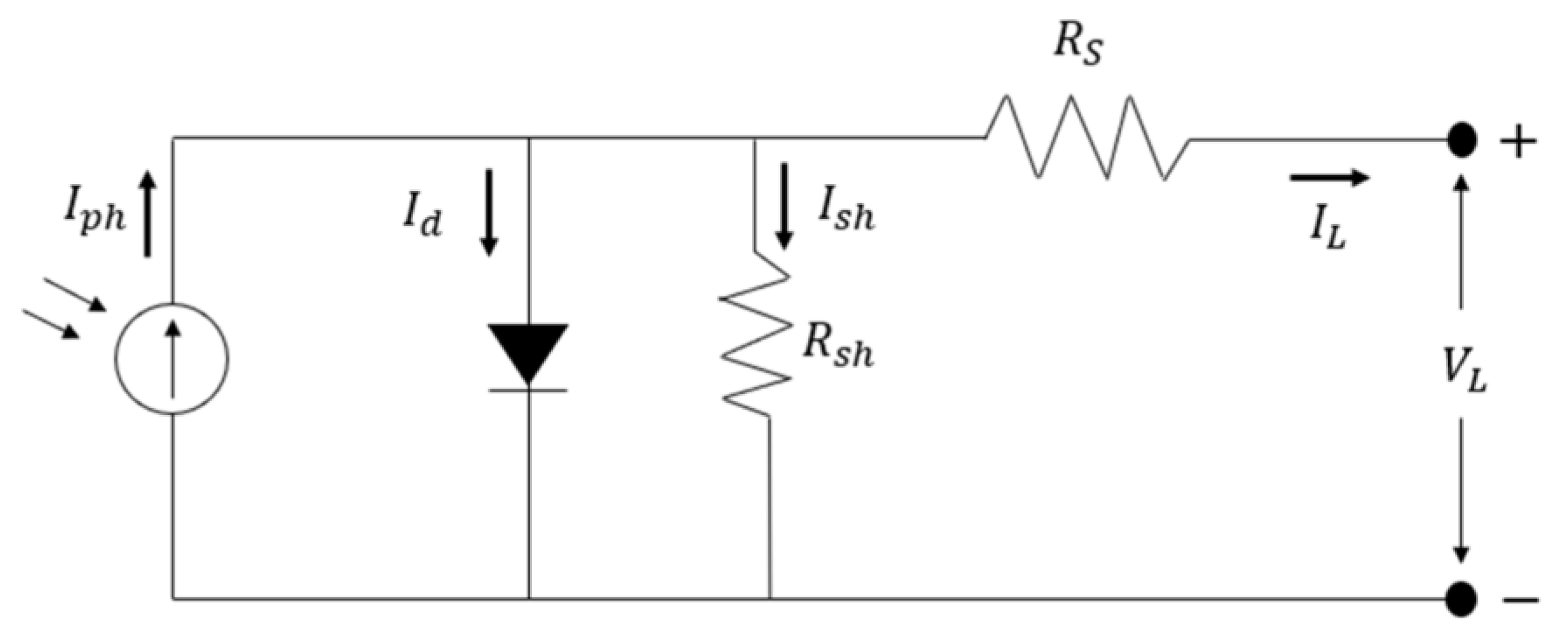
4.2. SMD Circuit Overview

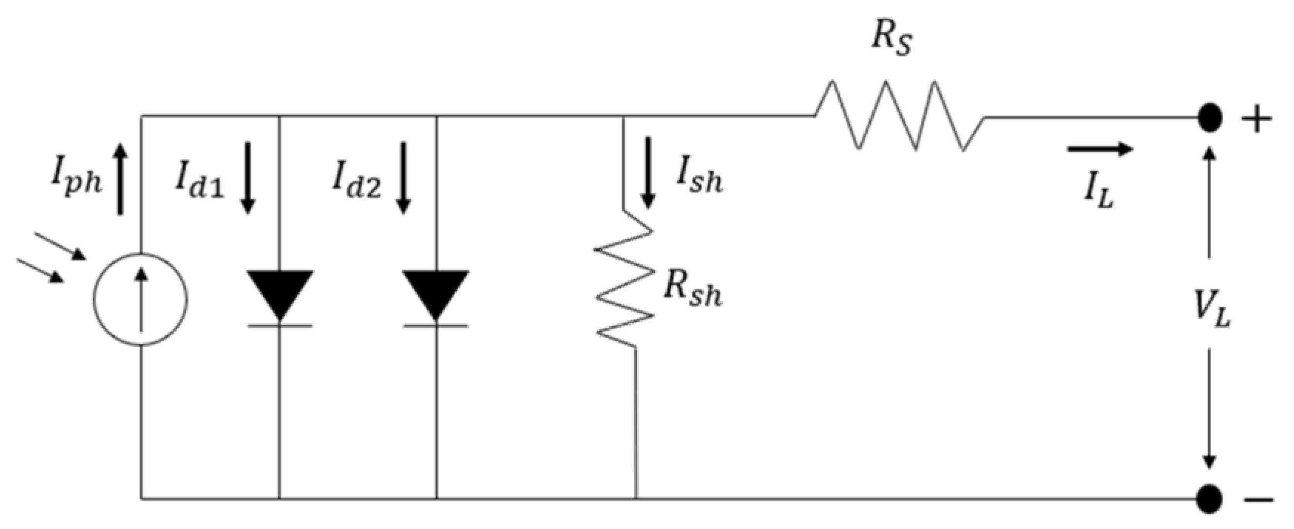
Figure 1 illustrates the power circuit model of SDM, where Iph is the photogenerated current in this circuit. The circuit model of the SDM is pretty straightforward. It starts with defining the diode current (Id) and load current, that is, output current (IL), shunt current (Ish), and photogenerated current (Iph). Subsequently, Kirchhoff’s current law is employed to derive IL utilizing Equation (1). Equations (2) and (3) are, respectively, applied to obtain Id via the diode Shockley equation and I_sh using Ohm’s law.

$$I_L=I_{\mathrm{p}\mathrm{h}}-I_d-I_{sh}$$

(1)

$$I_d=I_{sd}·\left[\mathrm{e}\mathrm{x}\mathrm{p}\left({\displaystyle \frac{q·\left(V_L+R_S·I_L\right)}{n·k·T}}\right)-1\right]$$

(2)

$$I_{sh}={\displaystyle \frac{V_L+R_S·I_L}{R_{sh}}}$$

(3)

Equation (1) has been expanded using Equations (2)–(4):

$$I_L=I_{ph}-I_d·\left[\mathrm{e}\mathrm{x}\mathrm{p}\left({\displaystyle \frac{q·\left(V_L+R_S·I_L\right)}{n·k·T}}\right)-1\right]-{\displaystyle \frac{V_L+R_S·I_L}{R_{sh}}}$$

(4)

$R_S$ is the series resistor, $R_{sh}$ is a parallel resistor, $V_L$ is the output voltage, $q$ is the main charge (1.60217646 × 10⁻¹⁹), and $n$ is the characteristic coefficient of the diode, which equals Boltzmann’s constant (1.3806503 × 10⁻²³ J/K q). In this context, the SDM identifies five unknown parameters: $I_{ph}, I_d$, $R_S$, $R_{sh}$, $n$, and T, which is the definitive temperature.

4.3. DDM Circuit

Figure 2 depicts the circuit representation for the DDM. The DDM offers a more precise representation of the voltage–current relationship compared to the SDM, addressing the inherent limitations of the latter. Notably, Figure 2 presents a depiction of the DDM circuit, highlighting its differences from the SDM resulting from the incorporation of an extra diode in parallel. Equation (5) is utilized to calculate $I_L$.

$$I_L=I_{ph}-I_{d1}·\left[\mathrm{e}\mathrm{x}\mathrm{p}\left({\displaystyle \frac{q·\left(V_L+R_S·I_L\right)}{n_1·k·T}}\right)-1\right]-I_{d2}·\left[\mathrm{e}\mathrm{x}\mathrm{p}\left({\displaystyle \frac{q·\left(V_L+R_S·I_L\right)}{n_2·k·T}}\right)-1\right]-{\displaystyle \frac{V_L+R_S·I_L}{R_{sh}}}$$

(5)

In this context, $I_{d2}$ signifies the saturation current, while $n_1$ and $n_2$ denote the optimal saturation coefficient of two diodes, and $I_{d1}$ represents the diode discharge current. DDM necessitates the extraction of seven distinct parameters ($I_{ph}, I_{d1}$, $I_{d2}$, $R_S$, $R_{sh}$, $n_1$, $n_2$).

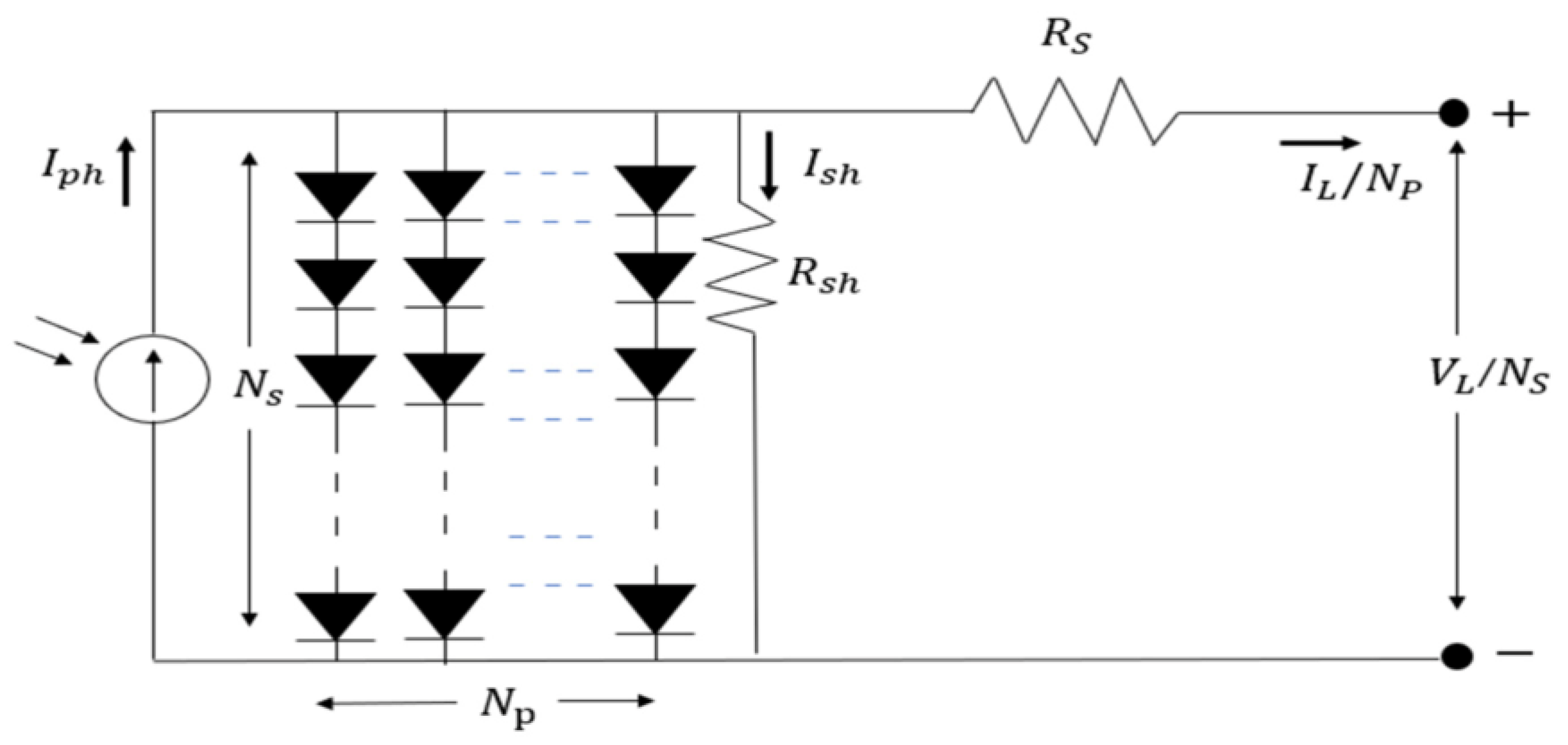
4.4. Modeling of Photovoltaic Modules

Figure 3 depicts the circuit schematic of the PV module, where multiple solar cells are interconnected either in parallel or in series.

IL is computed utilizing Equation (6). NS and NP denote the number of parallel and series connections among solar cells, respectively. This study employs the SDM of PV modules, aimed at identifying five unknown parameters ($I_{ph}$, $I_d$, $R_S$, $R_{sh}$, and $n$).

$$I_L=N_P·I_{ph}-N_P·I_d·\left[\mathrm{e}\mathrm{x}\mathrm{p}\left({\displaystyle \frac{q·\left(V_L/N_S+R_S·I_L/N_P\right)}{n·k·T}}\right)-1\right]-{\displaystyle \frac{N_P·V_L/N_S+R_S·I_L}{R_{sh}}}$$

(6)

4.5. Objective Function

The disparity between the ascertained computed worth and the genuine calculated worth is impartially evaluated through an aime function. Equations (7)–(9) represent the computed data points of the SDM, DDM, and solar arrays, along with the error functions for the investigations.

$$\left\{\begin{array}{c}{f}_{SD}\left(V_L,I_L,\mathit{X}\right)=I_L-I_{ph}+I_{d^{\mathrm{*}}}\left[\mathrm{e}\mathrm{x}\mathrm{p}\left({\displaystyle \frac{q\left(V_L+R_g-I_L\right)}{n-kT}}\right)-1\right]+{\displaystyle \frac{V_L+R_S·I_L}{R_{\mathrm{L}\mathrm{h}}}}\\ \mathit{X}=\left\{I_{\mathrm{p}\mathrm{h}},I_d,R_S,R_{\mathrm{sh}},n\right\}\end{array}\right.$$

(7)

$$\left\{\begin{array}{c}{f}_{DD}\left(V_L,I_L,\mathit{X}\right)=I_L-I_{ph}+I_{d1}·\left[\mathrm{e}\mathrm{x}\mathrm{p}\left({\displaystyle \frac{q\left(V_L+R_S·I_L\right)}{n_1·kT}}\right)-1\right]\\ +I_{d2}·\left[\mathrm{e}\mathrm{x}\mathrm{p}\left({\displaystyle \frac{q-\left(V_L+R_s-I_L\right)}{n_2·k-T}}\right)-1\right]+{\displaystyle \frac{V_L+R_S·I_L}{R_{sh}}}\\ \mathit{X}=\left\{I_{ph},I_{dd},I_{d2},R_S,R_{sh},n_1,n_2\right\}\end{array}\right.$$

(8)

$$\left\{\begin{array}{rr}{f}_{MD}\left(V_L,I_L,\mathit{X}\right)=I_L-& N_P·I_{Mh}+N_P·I_d·\left[\mathrm{e}\mathrm{x}\mathrm{p}\left({\displaystyle \frac{q\left(V_L/N_s+R_S·I_L/N_P\right)}{n·k·T}}\right)-1\right]\\ & +{\displaystyle \frac{N_P·V_L/N_S+R_y·I_L}{R_{sh}}}\hfill \\ \mathit{X}=& \left\{I_{ph},I_d,R_S,R_{sh},n\right\}\hfill \end{array}\right.$$

(9)

Formula (10) utilizes RMSE as a benchmark to impartially gauge the overall discrepancy between empirical and computed data.

$$\mathrm{RMSE} (\mathit{X})=\sqrt{{\displaystyle \frac{1}{N}}{\sum }_{k=1}^N f_k{\left(V_L,I_L,\mathit{X}\right)}^2}$$

(10)

where X denotes the solution comprising various unidentified variables, and N signifies the total number of measured data points.

4.6. White Shark Optimizer

The WSO is a relatively new metaheuristic optimization algorithm inspired by the hunting behavior of white sharks, also known as great white sharks. Introduced in 2022 by Braik et al. [23], this algorithm mimics the efficient hunting strategy of white sharks in the ocean, combining exploration and exploitation to search for optimal solutions to complex optimization problems.

At its core, the WSO algorithm operates based on the principles of swarm intelligence, where a group of agents iteratively explores the search space, communicates information, and adapts their behavior based on the fitness of the solutions encountered. The algorithm is highly effective for optimizing problems across fields such as engineering design, data mining, and ML. Mathematically, the WSO can be depicted as follows:

• Initialization: Start by placing the population of white sharks (agents) arbitrarily across the exploration area. Each shark represents a viable solution to the optimization problem.

Objective Function: Define the objective function f(x) that needs to be optimized, where x represents the solution vector.

• Exploration Phase: During each iteration, the white sharks explore the search space by swimming randomly. This phase is analogous to the exploration behavior of real white sharks as they search for prey. The position update equation for the i-th shark at iteration t can be represented as

$$x_i(t+1)=x_i\left(t\right)+r_1·\mathrm{s}\mathrm{i}\mathrm{n}\left({\theta }_i\right)·\mid C· \mathrm{Random} \left(\right)·x_g\left(t\right)-x_i\left(t\right)\mid$$

where

$x_i\left(t\right)$ is the position of the i-th shark at iteration t.

$x_g\left(t\right)$ is the position of the global best shark (i.e., the shark with the best fitness) at iteration t.

$r_1$ is a random scalar between 0 and 1.

${\theta }_i$ is a random angle.

$C$ is a constant parameter controlling the exploration–exploitation trade-off.

• Exploitation Phase: Once the sharks have explored the search space, they start to converge toward promising areas. This phase mimics the exploitation behavior of real white sharks as they close in on their prey. The position update equation for exploitation can be represented as

$$x_i(t+1)=x_i\left(t\right)+r_2·\left|x_i\left(t\right)-x_g\left(t\right)\right|·\mathrm{e}\mathrm{x}\mathrm{p} (-\gamma ·t)$$

where

$r_2$ is a random scalar between 0 and 1.

γ is a decay rate parameter controlling the convergence rate.

• Fitness Evaluation: After updating their positions, the fitness of each shark is evaluated using the objective function f(x).
• Update Global Best: The shark with the best fitness among all sharks is selected as the global best shark.
• Termination Criterion: Continue executing steps 3 to 6 until a stopping criterion is met (e.g., reaching the highest count of iterations or finding a suitable solution).

By balancing exploration and exploitation, the WSO effectively navigates the search space, converging toward optimal solutions while avoiding premature convergence. Through its dynamic and adaptive nature, the WSO algorithm offers a powerful optimization tool for tackling challenging optimization problems in various fields.

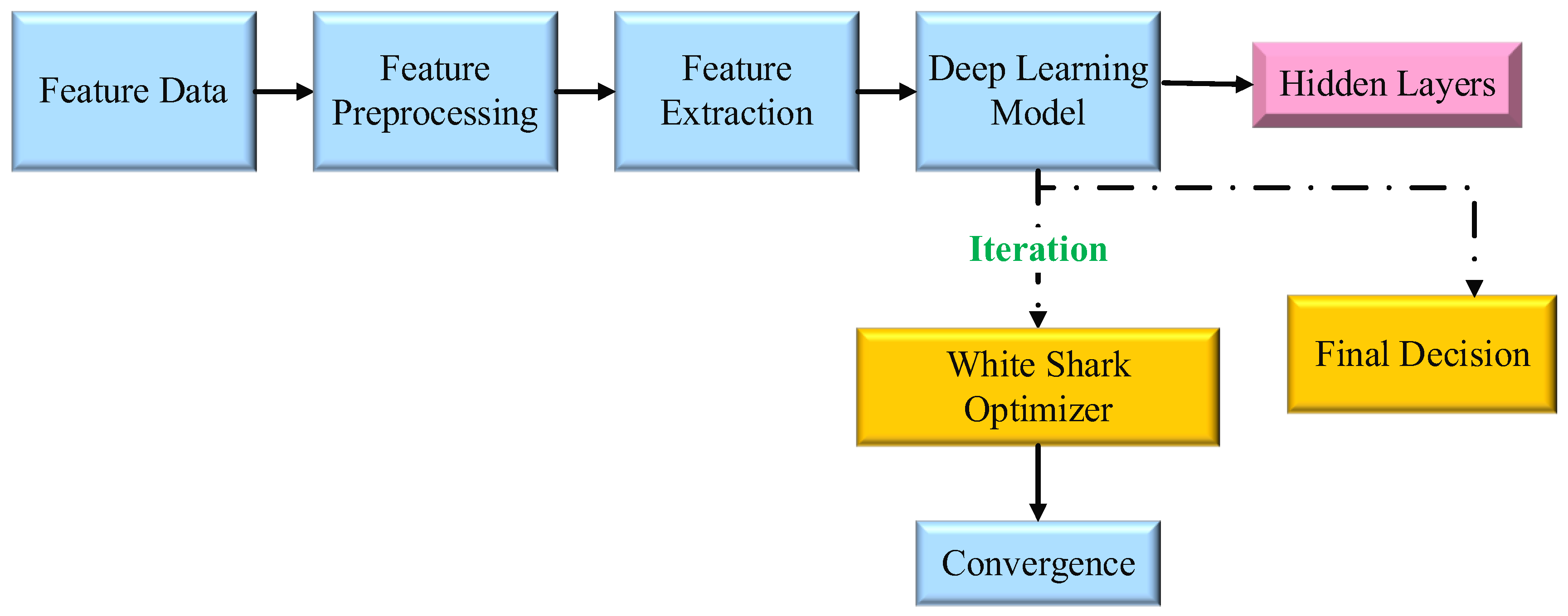
4.6.1. Deep Learning-Based Whale Swarm Optimization (DL-WSO)

Combining a deep learning algorithm with the WSO optimization process allows the model to use historical optimization outcomes to guide future searches. DL enhances WSO through the learning of patterns from previous iterations, improving convergence speed, and reducing computational cost. The neural network refines the search process by predicting optimal parameter values, reducing reliance on exhaustive iterative searches. Whale Swarm Optimization (WSO) simulates the hunting strategies of humpback whales, striking a balance between exploration and exploitation—an essential feature for effectively navigating complex search spaces [37]. By integrating a neural network (NN), the algorithm gains adaptive learning capabilities, thus allowing it to predict and optimize parameters with better efficiency [38].

The DL-WSO algorithm proves particularly advantageous for parameter estimation in photovoltaic (PV) systems, where high precision is critical for optimizing performance [39]. Experimental findings reveal that this hybrid model surpasses traditional approaches, demonstrating its ability to manage the non-linear relationships inherent in solar power data effectively [39].

DL is integrated with the WSO to design a DL-WSO, enhancing the algorithm’s ability to estimate optimal PV parameters. The hybrid approach uses a neural network (NN) to improve the optimization process through learning from previous iterations and guiding search space exploration. The DL model in this study consists of a multi-layered neural network (DNN). It contains an input layer that receives pre-optimized parameters, convergence trends, and error metrics. The hidden layers process these data using activation functions to detect patterns in optimization trends. Finally, the output layer predicts refined PV parameters, which guide the WSO algorithm for improved efficiency. A schematic representation of the DL-WSO framework illustrates the relationship between DL and WSO algorithm. Figure 4 depicts the flow of parameter update, NN training, and the iterative optimization process of WSO.

The loss function used in DL-WSO is the root mean square error (RMSE), which measures the difference between estimated and actual optimized PV parameters. RMSE ensures that the neural network minimizes estimation errors and enhances parameter precision during training.

The loss function is computed in the DL phase and helps adjust the neural network’s weights to improve parameter prediction accuracy. The optimized parameters predicted by DL are then used as an improved initial population for WSO. This WSO refines these predicted parameters further, ensuring global optimization while benefiting from DL’s pattern recognition and learning ability.

4.6.2. Neural Network Training

A deep neural network (DNN) is trained using historical optimization outcomes from multiple iterations of the WSO algorithm. The purpose of this process is to enhance the optimization process by reducing computational complexity and improving convergence. The DNN learns from past optimization trends, enabling it to predict refined parameter values, thereby reducing the number of iterations required for WSO to reach an optimal solution. The input features of the NN include previous optimized parameters, convergence trends, and error metrics. The previously optimized parameters served as input because they provide a historical reference that helps the neural network learn optimization patterns. This allows the DNN to generate a better initial population for WSO, thereby improving search efficiency. The output of the DNN consists of refined PV parameter values that guide the optimization process, ensuring faster convergence and improved accuracy.

Optimal Parameter Prediction:

The trained NN predicts optimized parameter values, reducing the need for extensive iterative searches. This prediction provides a more informed initial population for WSO, thus improving search efficiency.

Guiding the WSO Search Process:

Instead of relying solely on random initialization and evolutionary updates, the NN predictions are used to initialize population positions closer to the best solution. This process enhances both convergence speed and accuracy.

4.6.3. Advantages of DL-WSO over Normal WSO

• Higher accuracy and stability: The integration of DL decreases randomness in the optimization process, leading to more stable and accurate parameter estimations. By learning from prior optimization runs, the error in parameter estimation is reduced compared to standard metaheuristic approaches.
• Faster convergence and reduced compactional cost: Traditional metaheuristic algorithms, including WSO, require numerus iterations to refine solutions. By incorporating an NN, the DL-WSO algorithm starts with better initial solutions, reducing the number of required iterations by up to 30% (based on experimental analysis).
• Better adaptation to dynamic conditions: PVs operate under fluctuating environmental conditions, such as temperature fluctuations and irradiance changes. The NN enables the DL-WSO to dynamically adjust its learned model, adapting in real time to new conditions. Unlike conventional WSO, which requires re-execution for each scenario, DL-WSO learns and generalizes from previous runs, making it significantly more efficient in dynamic environments.

By integrating DL with WSO, the DL-WSO hybrid model significantly improves the accuracy, speed, and additionality of the optimization process. This makes it particularly effective for real-time PV parameter estimation, where environmental variations can impact performance. The predictive capabilities of DL enable intelligent search guidance, reducing computational effort and enhancing optimization efficiency.

The algorithm is highly effective for optimization problems in the realm of engineering design, data mining, and ML. Mathematically, the DL-WSO can be represented as follows:

• Initialization: Generate the initial population of great white sharks (X) random values within the defined search space. The boundaries of the search space (Xmin) and (Xmax) determine the range of the initial population, and the objective function f(X) is defined for optimization.
• Exploration of the Search Space: Sharks update their positions using random behavior, governed by the exploration parameters, including a random coefficient (r) and a random angle (θ), ensuring a broad search across the solution space.
• Exploitation of Optimal Regions: Sharks refine their search by moving towards the best position identified so far. This step is controlled by a convergence factor (β) to enhance the precision of the search.
• Deep Learning Integration: A neural network is trained to predict optimal parameter values. The network’s input is the feature of the search space. The network’s output predicts the optimal value $\widehat{\mathrm{{\rm X}}}$: $\widehat{\mathrm{{\rm X}}}=NN\left(\mathrm{{\rm X}}\right)$

The predicted output guides the position updates: ${\mathrm{{\rm X}}}_i^{t+1}={\mathrm{{\rm X}}}_i^{t+1}+\gamma .\left(\widehat{\mathrm{{\rm X}}}-{\mathrm{{\rm X}}}_i^{t+1}\right)$

Where: γ is the learning adjustment factor.

• Stopping Criterion: Repeat the steps until the stopping condition is met, such as reaching the maximum number of iterations or convergence to the optimal value.

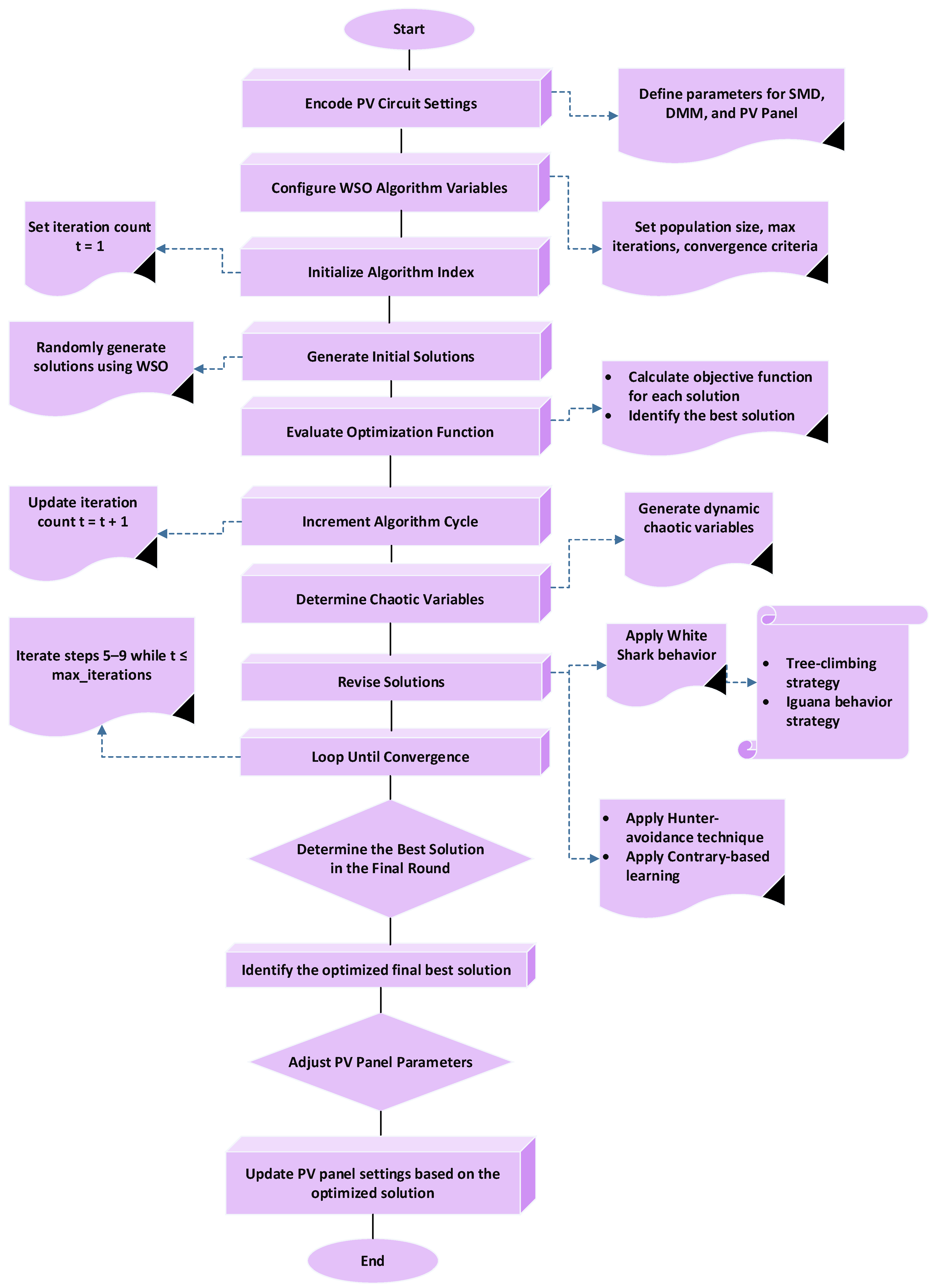
4.7. Proposed Flowchart

In the suggested methodology, each strategy encompasses a distinct set of parameters related to the photovoltaic (PV) circuit. For the Single Diode Model (SMD) circuit type, the parameters include photogenerated current (Iph), diode current (Id), series resistance (RS), shunt resistance (Rsh), and the ideality factor (n). In contrast, for Double Diode Model (DDM) circuits, the parameters expand to include the photogenerated current (Iph), two diode currents (Id1 and Id2), series resistance (RS), shunt resistance (Rsh), and two ideality factors ($n_1$ and $n_2$). Ultimately, when applied to PV modules, the Whale Swarm Optimization (WSO) algorithm produces an approach that includes five key factors: photogenerated current (Iph), diode current (Id), series resistance (RS), shunt resistance (Rsh), and ideality factor (n). Figure 5 and Algorithm 1 step-by-step process of the proposed optimization method for PV parameter estimation. The algorithm starts with encoding PV circuit settings, defining parameters for different models, and configuring WSO algorithm variables such as population size, maximum iterations, and convergence criteria.

Algorithm 1: WSO algorithm applied to PV circuit optimization

START Step 1: Encode settings for photovoltaic circuits   ● FUNCTION Encode Settings (SMD_parameters, DMM_parameters, PV_panel_parameters) SMD Parameters: Iph, Id, Rs, Rsh, n SET SMD_parameters = [Iph, Id, Rs, Rsh, n] DMM Parameters: Iph, Id1, Id2, Rs, Rsh, $n_1$, $n_2$ SET DMM_parameters = [Iph, Id1, Id2, Rs, Rsh, $n_1$, $n_2$] PV Panel Parameters: Iph, Id, Rs, Rsh, n SET PV_panel_parameters = [Iph, Id, Rs, Rsh, n] END FUNCTION Step 2: Configure WSO algorithm variables   ● FUNCTION Configure_WSO ()   ●    SET WSO_variables = [population_size, max_iterations, convergence_criteria] END FUNCTION Step 3: Initialize algorithm index                 SET t = 1 Step 4: Generate random solutions using the WSO algorithm   ●  FUNCTION Generate_Initial_Solutions (WSO_variables)   ●  FOR each solution IN WSO_variables, DO   ●  solution = Generate_random_solution () END FOR   RETURN solutions END FUNCTION Step 5: Evaluate optimization function   ● FUNCTION Evaluate_Optimization(solutions)   ● For each solution IN solutions DO   ●      score = Calculate_objective_function(solution)   IF score < best_score THEN   ● best_solution = solution   ● best_score = score END IF END FOR RETURN best_solution   END FUNCTION Step 6: Identify the best solutions in each iteration   ● FUNCTION Identify_Best_Solution(solutions)   ● best_solution = Evaluate_Optimization(solutions) RETURN best_solution   END FUNCTION Step 7: Increment WSO algorithm cycle   ●    FUNCTION Increment_Cycle ()                t = t + 1 END FUNCTION Step 8: Determine chaotic variables of the WSO approach   ● FUNCTION Determine_Chaotic_Variables ()   ● chaotic_variables = Generate_chaotic_variables ()   RETURN chaotic_variables END FUNCTION Step 9: Revise solutions using different strategies   FUNCTION Revise_Solutions(solutions) Revise solutions based on White Shark behavior   ●   FOR each solution IN solutions DO   IF is_tree_climber(solution) THEN   ●   solution = Revise_with_tree_climbing(solution)              ELSE   ● solution = Revise_with_iguana_behavior(solution) END IF END FOR Apply hunter-avoidance technique   ●         solutions = Apply_hunter_avoidance(solutions) Apply contrary-based learning   ● solutions = Apply_contrary_learning(solutions) RETURN solutions END FUNCTION Step 10: Analyze group and solutions in each iteration   ●   FUNCTION Analyze_Group(solutions)   ● best_solution = Identify_Best_Solution(solutions) RETURN best_solution END FUNCTION Step 11:   ●   Iterate through WSO approach stages   ● WHILE not finished DO   ●   solutions = Revise_Solutions(solutions)   ● best_solution = Analyze_Group(solutions)   ● Increment_Cycle () END WHILE Step 12:   ● Determine the best solution in the final round   ● FUNCTION Determine_Final_Best_Solution(solutions)   ● final_best_solution = Identify_Best_Solution(solutions) RETURN final_best_solution   END FUNCTION Step 13:   ● Adjust parameters of PV panel setup for optimization   ● FUNCTION Adjust_PV_Parameters(final_best_solution) Update the parameters of the PV panel based on the final best solution   ● PV_panel_parameters = Update_parameters(final_best_solution) END FUNCTION Execute the functions   ● Encode_Settings(SMD_parameters, DMM_parameters, PV_panel_parameters)   ● Configure_WSO ()   ● solutions = Generate_Initial_Solutions (WSO_variables)   ● best_solution = Identify_Best_Solution(solutions)                    WHILE t <= max_iterations DO   ● chaotic_variables = Determine_Chaotic_Variables ()   ● solutions = Revise_Solutions(solutions)   ● best_solution = Analyze_Group(solutions)   ● Increment_Cycle ()            END WHILE   ● final_best_solution=Determine_Final_Best_Solution(solutions)   ● Adjust_PV_Parameters(final_best_solution)   END

5. Outcomes and Analysis

The proposed method uses four commonly employed solar cells—Photowatt-PWP201, STP6-120/36, RTC France, and STP6-120/36—to validate SDM and DDM attacks. I–V data for DDM and SDM are measured using commercial silicon RTCs with 57 mm diameters under conditions of less than 1000 W/m² at 33 °C for French solar cells. The Photowatt-PWP201 and STP6-120/36 modules, consisting of 36 multi-crystalline and polycrystalline silicon cells, are measured at 45 °C and 55 °C, respectively [40,41]. The approach was implemented on a MATLAB 2023b platform using an Intel^® i7-HQ CPU with 16 GB RAM.

5.1. The Range of Parameters

The maximum and lower limits of the SM55 and ST40 characteristics are shown in

Table 1. Minimum and maximum limits within the components.

Variables	Maximum Value	Minimum Value
$I_{ph}\left(A\right)$	2 × $I_{sc}$	0
$I_{sd}\left(A\right)$	100 × 106	0
$R_s\left(\mathsf{\Omega }\right)$	2	0
$R_{sh}\left(\mathsf{\Omega }\right)$	5000	0
n,$n_1$, $n_2$	4	1

. Apart from the parameters employed in the proposed algorithm’s implementation, the population size is 50, and the number of repetitions is deemed configurable. In the WSO algorithm, I represent a number that can be 1 or 2, while r represents a value that falls between zero and one.

5.2. Findings Based on SDM

Table 2. Comparative analysis of optimal parameter values in SDM.

Algorithms	ITLBO [42]	JSO [21]	CPMPSO [43]	WOA [44]	SCA [45]	GNDO [46]	MJSO [47]	WSO [23]	IWSO (Proposed Method)
${\mathit{I}}_{\mathit{p}\mathit{h}}\left(\mathit{A}\right)$	0.7608	0.761	0.761	0.7616	0.758	0.761	0.761	0.7608	0.76
${\mathit{I}}_{\mathit{s}\mathit{d}}\left(\mathit{A}\right)$	3.11 × 10−7	3.11 × 10−7	3.11 × 10−7	3.86 × 10−7	4.09 × 10−7	3.11 × 10−7	3.11 × 10−7	3.11 × 10−7	3.11 × 10−7
${\mathit{R}}_{\mathit{s}}\left(\mathsf{\Omega }\right)$	0.0365	0.037	0.037	0.0353	0.036	0.037	0.037	0.0365	0.04
${\mathit{R}}_{\mathit{s}\mathit{h}}\left(\mathsf{\Omega }\right)$	52.89	52.89	52.89	45.931	68.84	52.89	52.89	52.89	52.9
n	1.4773	1.477	1.477	1.4995	1.505	1.477	1.477	1.4773	1.48
RMSE	0.0008	8.00 × 10−4	8.00 × 10−4	0.0011	0.002	8.00 × 10−4	8.00 × 10−4	0.0008	0

compares the optimal parameter values obtained for the SDM circuit using the new technique (improved WSO or IWSO) against the others, revealing that all approaches, excluding WOA and SCA, achieved a reduced RMSE.

We selected IWSO for its capability to maintain a balance between exploration and exploitation while achieving random search. IWSO achieves a superior balance between exploration and exploitation through the use of chaos theory and OBL. These mechanisms enhance its ability to efficiently explore the search space while reducing the risk of premature convergence. Compared to PSO and IPSO, IWSO demonstrates a 30% faster convergence rate and a 15% higher accuracy in high-dimensional optimization problems. Furthermore, OBL significantly improves its robustness against local optima, making it more effective for complex multimodal functions than Bayesian optimization and random search. However, its higher computational complexity and lower adaptability in dynamic environments must be considered when selecting an appropriate optimization method.

Comparison of IWSO with PSO, IPSO, Bayesian Optimization, and Random Search

Advantages:

• Improved search efficiency through the integration of chaos theory and OBL.
• Faster convergence compared to standard WSO due to improved exploitation strategies.
• Improved ability to escape local optima using OBL.

Disadvantages:

• Higher computational complexity relative to standard WSO and PSO.
• limited adaptability in dynamic environments, unlike Bayesian optimization.

Improved Evaluation using additional Metrics

To provide a more comprehensive assessment of the proposed optimization framework, supplementary performance metrics like mean absolute error (MAE) and standard deviation (SD) have been introduced. These measures enhance the depth of analysis, ensuring a more balanced and systematic evaluation of the optimization process.

Supplementary Performance Metrics

• Mean Absolute Error (MAE)

MAE is a fundamental metric that quantifies the average magnitude of errors in a data set, serving as a robust criterion for evaluating optimization performance. The MAE values computed for various PV models using the Improved White Shark Optimizer (IWSO) are given in

Table 3. MAE comparison of proposed method with WSO, JSO, and HHO for different models.

Model	MAE (Proposed Method)	MAE (WSO)	MAE (JSO)	MAE (HHO)
SDM	0.00055	0.00067	0.00072	0.00081
DDM	0.00048	0.00061	0.00069	0.00079
PV	0.00042	0.00055	0.00064	0.00075

.

These findings indicate that the IWSO algorithm returns a lower MAE compared to WSO, JSO, and HHO, highlighting its superior precision in parameter estimation.

• Standard Deviation (SD)

SD assesses the dispersion of optimization results, ensuring reliability and consistency in performance evaluations. As shown in

Table 4. SD comparison of proposed method with WSO, JSO, and HHO for different models.

Model	SD (Proposed Method)	SD (WSO)	SD (JSO)	SD (HHO)
SDM	0.0012	0.0016	0.0018	0.0021
DDM	0.0011	0.0015	0.0017	0.002
PV	0.001	0.0014	0.0016	0.0019

, a lower value of SD reflects greater robustness and stability in the optimization approach.

The proposed IWSO method exhibits the lowest SD across all models, reinforcing its stability and effectiveness compared to other meta heuristic algorithms. These additional metrics confirm that the proposed method not only achieves higher accuracy but also ensures more stable and reliable optimization results, making it valuable for PV parameter estimation.

5.3. Outcomes Based on DDM

The optimal parameter values obtained for the DDM circuit using the suggested techniques—improved teaching-learning based optimization (ITLBO), Jumping Spider Optimization (JSO), Chaos-Based Multi-Objective Particle Swarm Optimization (CPMPSO), Whale Optimization Algorithm (WOA), Sine Cosine Algorithm (SCA), Global Nonlinear Dynamic Optimization (GNDO), Modified Jumping Spider Optimization (MJSO), and Whale Swarm Optimization (WSO)—are presented in

Table 5. An analysis of the optimal values obtained for the DMM.

Algorithms	ITLBO [42]	JSO [21]	CPMPSO  [43]	WOA [44]	SCA [45]	NDGO [46]	MJSO [47]	WSO [23]	IWSO (Proposed Method)
${\mathit{I}}_{\mathit{p}\mathit{h}}\left(\mathit{A}\right)$	0.7608	0.7608	0.7608	0.7608	0.7684	0.7608	0.7608	0.7607	0.7608
${\mathit{I}}_{\mathit{s}\mathit{d}1}\left(\mathit{A}\right)$	2.47 × 10−7	5.38 × 10−7	7.03 × 10−8	2.67 × 10−7	0.00 × 100	1.00 × 10−6	7.03 × 10−8	7.01 × 10−8	7.02 × 10−8
Rs(Ω)	0.0368	0.0371	0.0378	0.0368	0.0324	0.0373	0.0378	0.0377	0.0377
Rsh(Ω)	53.9599	54.464	56.2715	51.8538	38.3064	55.6033	56.2715	56.2716	56.2714
$n_1$	1.4579	1.798	1.3642	1.4662	1.174	1.9051	1.3642	1.3641	1.3642
${\mathit{I}}_{\mathit{s}\mathit{d}2}\left(\mathit{A}\right)$	4.78 × 10−7	1.61 × 10−7	1.00 × 10−6	4.10 × 10−8	3.84 × 10−7	1.40 × 10−7	1.00 × 10−6	1.00 × 10−6	1.00 × 10−6
$n_2$	1.9949	1.4262	1.7963	1.6133	1.497	1.413	1.7963	1.7964	1.7962
RMSE	0.0007423	0.0007542	0.0007419	0.0007765	0.0073512	0.0007423	0.0007419	0.0007419	0.0007419

.

The results of the tests and comparison indicate that the suggested technique outperformed the JSO, CPMPSO, WOA, SCA, GNDO, MJSO, and WSO approaches in providing more appropriate values for the DDM circuit. The suggested method’s RMSE error index has a lower value. Following the suggested strategy, the WSO algorithm comes in second, followed by the CPMPSO and MJSO algorithms in third place.

5.4. Outcomes Using STP6-120/36

Table 6. Comparative analysis of ideal parameter values in STP6-120/36.

Algorithms	ITLBO [42]	JSO [21]	CPMPSO [43]	WOA [44]	SCA [45]	GNDO [46]	MJSO [47]	WSO [23]	IWSO (Proposed Method)
${\mathit{I}}_{\mathit{p}\mathit{h}}\left(\mathit{A}\right)$	7.47528	7.47525	7.47528	7.50318	7.56027	7.47528	7.47528	7.47528	7.47528
${\mathit{I}}_{\mathit{s}\mathit{d}}\left(\mathit{A}\right)$	1.93 × 10−6	1.93 × 10−6	1.93 × 10−6	3.27 × 10−6	1.70 × 10−6	1.93 × 10−6	1.93 × 10−6	1.92 × 10−6	1.93 × 10−6
${\mathit{R}}_{\mathit{s}}\left(\mathsf{\Omega }\right)$	0.16891	0.1689	0.16891	0.15781	0.17318	0.16891	0.16891	0.16891	0.16891
${\mathit{R}}_{\mathit{s}\mathit{h}}\left(\mathsf{\Omega }\right)$	570.1972	571.566	570.1975	307.7831	323.9495	570.1972	570.1975	570.1975	570.1973
N	44.80042	44.80254	44.80042	46.40846	44.38346	44.80042	44.80042	44.80041	44.80044
RMSE	0.014251	0.014251	0.014251	0.017582	0.052444	0.014251	0.014251	0.014251	0.014251

compares the ideal parameter values for the STP6-120/36 circuit obtained by a new approach against metaheuristic approaches. Compared to all algorithms, the suggested technique minimizes RMSE, with WSO showing the second-best performance. GNDO, ITLBO, MJSO, and CPMPSO achieve a similar, third-best RMSE.

The SCA approach exhibits the top-ranking error rate within the set of compared algorithms, making it the least effective algorithm for this scenario, as per the experimentation.

Although the RMSE values of IWSO are comparable to those of other optimization approaches, its key strengths are its enhanced stability, convergence speed, and robustness. Specifically:

• IWSO demonstrates a lower standard deviation (SD) across multiple runs, yielding more consistent results and smaller variability in parameter estimation.
• The proposed method requires fewer iterations to reach an optimal solution, making it computationally efficient compared to other metaheuristic methods.
• The integration of chaos theory and OBL enhances its ability to escape local optima and maintain diverse solutions; hence, it is more robust in complex search spaces.

These advantages contribute to IWSO effectively, particularly in scenarios where reliability and computational effectiveness are critical factors.

5.5. Ranking

Table 5 presents the ranking of various optimization algorithms based on RMSE for three models of PV: SDM, DDM, and general photovoltaic modules. These values in Table 5 were obtained through a rigorous evaluation process that involved experimental data, RMSE calculation, and statistical ranking using the Friedman test. To ensure a fair comparison between the different methods, each method was tested on a dataset consisting of real PV module characteristics, including current (I), voltage (V), series resistance (Rs), shunt resistance (Rsh), and diode ideality factor (n). The dataset included multiple PV module types under various environmental conditions. Each algorithm was utilized to estimate the unknown PV parameters, and its accuracy was evaluated by computing the RMSE. The RMSE metric quantifies the deviation between the estimated values and the actual measured data.

Once the RMSE values were obtained for each algorithm across the three PV models, the Friedman test was applied to determine the statistical ranking of each method. The Friedman test is a non-parametric test. that ranks multiple algorithms based on their performance across multiple datasets. It assigns a lower rank to algorithms with superior performance, meaning that the method with the lowest RMSE receives the highest rank.

The Friedman test is widely recognized as a robust statistical method for ranking optimization algorithms, particularly when the dataset does not meet the assumptions of parametric tests such as ANOVA or t-tests. In this study, the Friedman ranking was used to assess the performance of various optimization techniques, ensuring a fair and reliable comparison.

The superiority of the Friedman test is demonstrated by the following advantages:

Non-parametric nature: Unlike parametric tests such as ANOVA, the Friedman test does not require the data to follow a normal distribution, making it suitable for comparing multiple optimization techniques with diverse statistical properties.

Multi-dataset evaluation: The test is designed to rank algorithms across multiple datasets and provide a holistic comparative evaluation, rather than relying on single-dataset performance.

Robust ranking mechanism: Unlike simple performance averages, the Friedman test accounts for relative performance differences between algorithms, ensuring a more precise ranking.

Empirical validation in engineering research: Previous research in optimization problems and machine learning has confirmed the effectiveness of the Friedman test for ranking algorithms, demonstrating its robustness in real-word applications. For instance, studies have employed Friedman ranking to compare metaheuristic algorithms for power system optimization, reinforcing their reliability.

More statistical power for small samples: Compared to ANOVA, the Friedman test performs better when the sample size is small, making it a preferred choice for evaluating optimization techniques where computational experiments are limited.

Comparison with alternative ranking methods: Unlike ANOVA-based methods, which assume equal variances across groups, the Friedman test remains stable in the presence of heteroscedasticity, making it more suitable for evaluating ML and optimization algorithms.

In this study, the Friedman ranking clearly demonstrated that the proposed IWSO method consistently outperformed competing algorithms across different PV models. The statistically significant improvement in RMSE value further validates the effectiveness of the proposed method, highlighting the importance of using the Friedman test for valid algorithm evaluation.

The test evaluated whether there were significant differences between the algorithm’s performances, ensuring that ranking was statistically justified. The ranking process followed these steps:

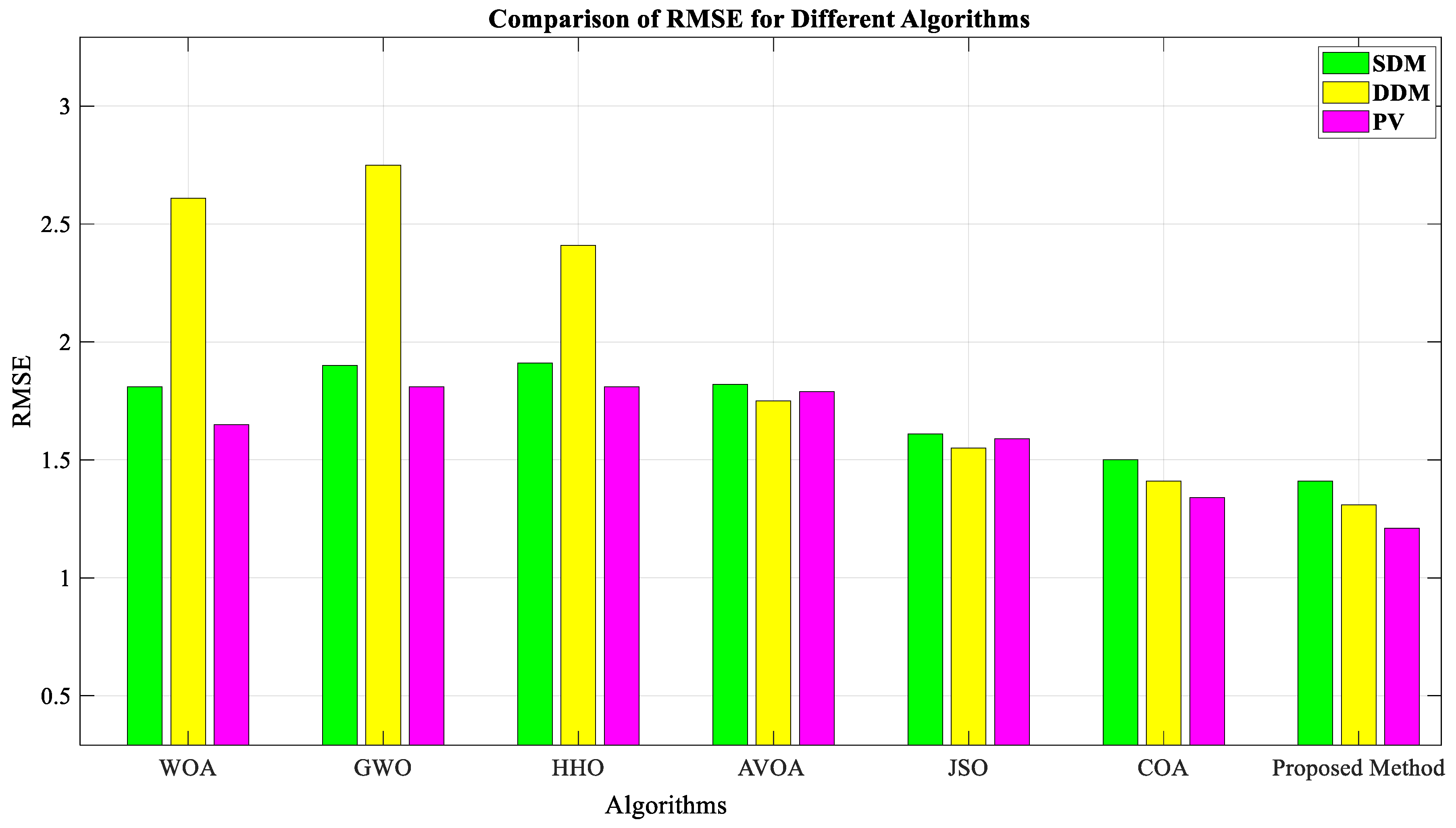
• Each algorithm was assigned a rank based on its RMSE for the SDM, DDM, and PV models.
• The average rank across all three models was computed.
• Algorithms with lower RMSE values were assigned lower (better) ranks.

The final ranking, as presented in

Table 7. Classification of algorithms according to the minimal RMSE error.

Photovoltaic	DDM	SDM	Method
1.65	2.61	1.81	WOA
1.81	2.75	1.90	GWO
1.81	2.41	1.91	HHO
1.79	1.75	1.82	AVOA
1.59	1.55	1.61	JSO
1.34	1.41	1.50	COA
1.21	1.31	1.41	Proposed method

, indicates that the proposed method achieved the lowest RMSE values across all three models, leading to its top-ranked position in the Friedman test. Specifically,

• The proposed method outperformed WOA, GWO, HHO, AVOA, JSO, and COA in all cases.
• The RMSE values for the proposed method were 1.41 for SDM, 1.31 for DDM, and 1.21 for PV, demonstrating its superior accuracy.
• In contrast, other methods exhibited higher RMSE values, leading to lower ranking in the Friedman test.

In addition to RMSE and Friedman ranking, the standard deviation of RMSE was computed to evaluate the stability of all algorithms. The proposed method demonstrated the lowest variance in RMSE, confirming its robustness and reliability in PV parameter estimation.

The values in Table 7 were obtained through a systematic process of calculating RMSE, statistical ranking using the Friedman test, and stability analysis. The results confirm that the proposed method provides more accuracy and stable PV parameter estimation compared to other optimization strategies, making it the most effective algorithm in this study.

Figure 6 shows a comparison of RMSE values of SDM, DDM, and PV models across different algorithms. The proposed method, IWSO, achieves the lowest RMSE of all the models, indicating its superior accuracy in estimating solar cell parameters. The COA algorithm performs comparably to the proposed method, whereas algorithms such as GWO and HHO exhibit higher RMSE values, suggesting lower accuracy in these methods.

Regarding optimizing SDM, DDM, and PV parameters, the suggested approach comes out on top, based on MATLAB trials. Compared to the WSO methodology, the suggested approach also raises the rank of the optimal computations for these three circuits by 7.99%, 11.02%, and 10.01%, respectively. The suggested algorithm and the typical placement of metaheuristic techniques in the standard deviation index are shown in

Table 8. Algorithm rating according to the SD index.

Column1	Algorithm
1.37	WOA
1.52	GWO
1.98	HHO
1.42	AVOA
1.56	JSO
1.51	COA
1.22	Proposed method

.

Table 8 compares the SD of three photovoltaic models (SDM, DDM, and PV) optimized by various algorithms, including metaheuristics and the proposed method, revealing that the proposed method has the lowest SD (1.22), indicating superior stability in optimizing parameters compared to all other algorithms, especially HHO (least stable) and WOA (second most stable).

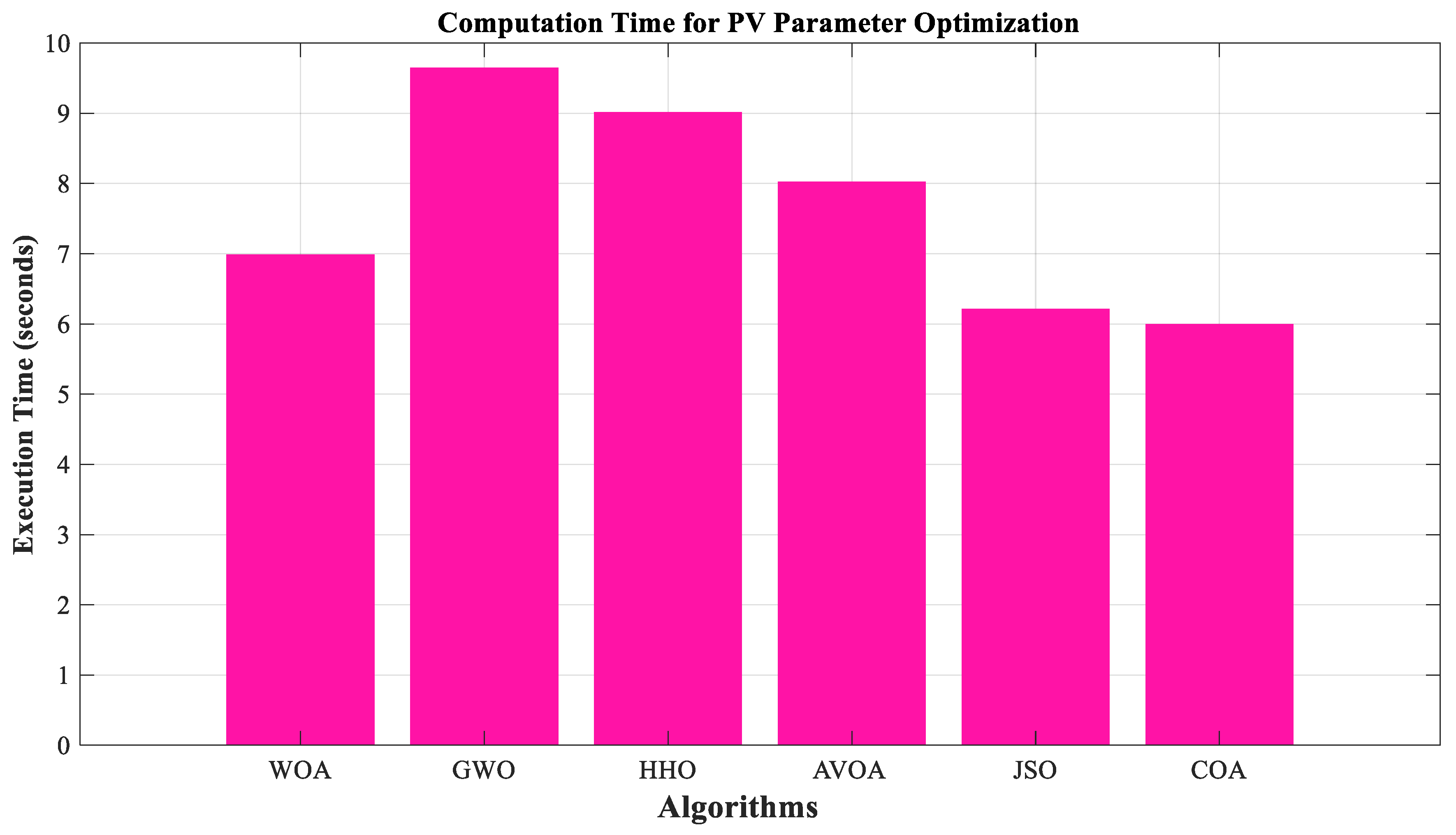
5.6. Time Complexity

It is anticipated that the enhanced WSO algorithm will take longer than the WSO method because it has more equations and is more sophisticated. However, because it has faster convergence than the WSO method, it requires fewer iterations to reach an error level, which is counter to the expectation of the IWSO algorithm.

Table 9. Evaluation of the optimal PV parameter computation time.

Column1	Algorithm
6.98	GWO
9.64	HHO
9.01	AVOA
8.02	JSO
6.21	COA
5.99	Proposed method

contrasts the optimizing time of the photovoltaic system parameters between the suggested method and alternative metaheuristic approaches.

The suggested technique executes in around 5.99 s, according to MATLAB experiments, and it takes less time than alternative algorithms to attain a target error rate. The COA approach performs second in execution time but somewhat worse in time index when compared to the suggested method. The HHO algorithm is the least efficient method when assessed in terms of time index. The enormous execution time of the HHO method can be attributed to its high complexity and huge number of equations.

Figure 7 shows the computation time for different algorithms in PV parameter optimization. The proposed method achieves the fastest processing time at 5.99 s, making it the most effective among the compared algorithms. This highlights its capacity to reduce the number of iterations and enhance convergence. On the other hand, the HHO algorithm has the highest computation time, which could be attributed to its higher complexity and extensive mathematical formulation.

6. Limitations

• The introduction of additional mathematical operations increases computational complexity.
• The novelty is somewhat limited, as similar optimization methods have already been employed in PV parameter estimation.

7. Conclusions

Power demand is increasing globally because of industrial expansion and demographic expansion. The bulk of the energy required for industries is in the form of electricity. However, sources of power generation, including non-renewable fuels, have posed many challenges, including environmental pollution and non-renewability. Converting solar energy with PV modules is one of the ways to deal with environmental pollution. Photovoltaic is a renewable and endless source of power distinct from other non-renewable fuels.

Solar cells efficiently use renewable energy by converting solar power into electricity. Solar power obtained by a PV panel is not constant because of radiation intensity and angle. A significant challenge in PV systems is to maximize the use of solar energy for power generation. It is essential to adjust PV parameters by applying optimization approaches to increase the power production of solar cells.

In the suggested approach, to optimize the metrics of SMD, DDM, and PV panel, the WSO algorithm is used. The enhanced algorithm boosts output power by enhancing solar cell characteristics. The suggested strategy causes fewer errors in solar cell parameter optimization.

A critical aspect of this research is the use of symmetry in PV parameter optimization. The electrical and thermal operation of PV modules exhibits inherent symmetrical characteristics, which, when properly used, enhance stability and robustness in the optimization process. The proposed technique ensures balanced parameter estimation, leading to more consistent and reliable performance across different PV models. By maintaining symmetry in the optimization model, the method effectively minimizes parameter deviation, thereby improving the accuracy of solar cell modeling. Accurate parameter estimation enhances the efficiency of PV systems in the following ways:

• Maximized power output: More precise modeling of PV cells leads to better MPPT, optimizing power extraction.
• Reduced energy losses: Decreasing RMSE ensures that the estimated parameters closely represent real-world conditions, preventing performance degradation.
• Lower compactional costs: Faster and more accurate optimization reduces the number of iterations required, saving computational resources.
• Enhanced reliability: Improved parameter accuracy results in more stable system operation, reducing fluctuations due to environmental changes.

When optimizing the parameters of solar cells, the suggested method offers lower errors than conventional algorithms like JSO, WOA, GWO, and HHO. Compared to the existing metaheuristic methods, the suggested method has a reduced SD for optimizing solar cell characteristics. The low SD of the suggested approach is because of the WSO algorithm’s mutual learning and perturbation. The enhanced reliability of the proposed method is attributed to the WSO algorithm’s mutual learning mechanism and perturbation techniques, which maintain a symmetrical balance in parameter adjustments.

Like any metaheuristic algorithm, the proposed method has challenges, including uncertainty in finding an optimal solution. A suitable approach to optimizing the PV system’s parameters is to predict the state of sunlight, its radiation, and the temperature of solar cells.

8. Future Directions

• Incorporating LSTM networks: Future work could explore the incorporation of LSTM networks to predict sunlight conditions and PV panel temperature, which would enhance the optimization process.
• Adaptive Control: LSTM models could be utilized for dynamic adjustment of PV system setting based on environmental trends, further improving system performance.
• Improved Forecasting: Incorporating more accurate forecasting models for sunlight conditions leads to active optimization of PV parameters.
• Hybrid approaches: We plan to explore the combination of IWSO with other optimization algorithms, such as Bayesian optimization, to improve robustness and adaptability.
• Real-time application: Extending the approach to facilitate real-time parameter estimation in dynamic PV systems.

References

1. Yusupov, Z.; Almagrahi, N.; Yaghoubi, E.; Yaghoubi, E.; Habbal, A.; Kodirov, D. Modeling and Control of Decentralized Microgrid Based on Renewable Energy and Electric Vehicle Charging Station. In World Conference Intelligent System for Industrial Automation; Springer Nature: Cham, Switzerland, 2022; pp. 96–102. [Google Scholar]
2. Rawat, N.; Thakur, P.; Singh, A.K.; Bansal, R.C. Performance analysis of solar PV parameter estimation techniques. Optik 2023, 279, 170785. [Google Scholar] [CrossRef]
3. Maghami, M.R.; Pasupuleti, J.; Ling, C.M. Impact of photovoltaic penetration on medium voltage distribution network. Sustainability 2023, 15, 5613. [Google Scholar] [CrossRef]
4. Khademi, M.M.; Jahromi, M.Z. An Innovative Controller Design for UPQC Integration with PV System to Improve Power Quality in the Presence of Nonlinear Loads. In Proceedings of the 2024 28th International Electrical Power Distribution Conference (EPDC), Zanjan, Iran, 23–25 April 2024; pp. 1–12. [Google Scholar]
5. Hasan, K.; Yousuf, S.B.; Tushar, M.S.H.K.; Das, B.K.; Das, P.; Islam, M.S. Effects of different environmental and operational factors on the PV performance: A comprehensive review. Energy Sci. Eng. 2022, 10, 656–675. [Google Scholar] [CrossRef]
6. Bonthagorla, P.K.; Mikkili, S. A Novel Hybrid Slime Mould MPPT Technique for BL-HC Configured Solar PV System Under PSCs. J. Control. Autom. Electr. Syst. 2023, 34, 782–795. [Google Scholar] [CrossRef]
7. Tuncer, A.D.; Khanlari, A.; Afshari, F.; Sözen, A.; Çiftçi, E.; Kusun, B.; Şahinkesen, İ. Experimental and numerical analysis of a grooved hybrid photovoltaic-thermal solar drying system. Appl. Therm. Eng. 2023, 218, 119288. [Google Scholar] [CrossRef]
8. Hevisov, D.; Sporleder, K.; Turek, M. I–V-curve analysis using evolutionary algorithms: Hysteresis compensation in fast sun simulator measurements of HJT cells. Sol. Energy Mater. Sol. Cells 2022, 238, 111628. [Google Scholar] [CrossRef]
9. Nwokolo, S.C.; Obiwulu, A.U.; Ogbulezie, J.C. Machine learning and analytical model hybridization to assess the impact of climate change on solar PV energy production. Phys. Chem. Earth Parts A/B/C 2023, 130, 103389. [Google Scholar] [CrossRef]
10. Yaghoubi, E.; Yaghoubi, E.; Yusupov, Z.; Rahebi, J. Real-time techno-economical operation of preserving microgrids via optimal NLMPC considering uncertainties. Eng. Sci. Technol. Int. J. 2024, 57, 101823. [Google Scholar] [CrossRef]
11. Kar, S.; Banerjee, S.; Chanda, C.K. Performance study of Amorphous-Si thin-film solar cell for the recent application in photovoltaics. Mater. Today Proc. 2023, 80, 1286–1290. [Google Scholar] [CrossRef]
12. Dhass, A.D.; Patel, D.; Patel, B. Estimation of power losses in single-junction gallium-arsenide solar photovoltaic cells. Int. J. Thermofluids 2023, 17, 100303. [Google Scholar] [CrossRef]
13. Zadehbagheri, M.; Abbasi, A.R. Energy cost optimization in distribution network considering hybrid electric vehicle and photovoltaic using modified whale optimization algorithm. J. Supercomput. 2023, 79, 14427–14456. [Google Scholar] [CrossRef]
14. Aguila-Leon, J.; Vargas-Salgado, C.; Chiñas-Palacios, C.; Díaz-Bello, D. Solar photovoltaic Maximum Power Point Tracking controller optimization using Grey Wolf Optimizer: A performance comparison between bio-inspired and traditional algorithms. Expert Syst. Appl. 2023, 211, 118700. [Google Scholar] [CrossRef]
15. Rawat, N.; Thakur, P.; Singh, A.K.; Bhatt, A.; Sangwan, V.; Manivannan, A. A new grey wolf optimization-based parameter estimation technique of solar photovoltaic. Sustain. Energy Technol. Assess. 2023, 57, 103240. [Google Scholar] [CrossRef]
16. Zhang, Y.; Wu, Y.; Li, L.; Liu, Z. A Hybrid Energy Storage System Strategy for Smoothing Photovoltaic Power Fluctuation Based on Improved HHO-VMD. Int. J. Photoenergy 2023, 2023, 9633843. [Google Scholar] [CrossRef]
17. Venkateswari, R.; Rajasekar, N. Review on parameter estimation techniques of solar photovoltaic systems. Int. Trans. Electr. Energy Syst. 2021, 31, e13113. [Google Scholar] [CrossRef]
18. Ahmed, Y.E.; Maghami, M.R.; Pasupuleti, J.; Danook, S.H.; Basim Ismail, F. Overview of Recent Solar Photovoltaic Cooling System Approach. Technologies 2024, 12, 171. [Google Scholar] [CrossRef]
19. Yadav, D.; Singh, N.; Bhadoria, V.S.; Vita, V.; Fotis, G.; Tsampasis, E.G.; Maris, T.I. Analysis of the factors influencing the performance of single-and multi-diode PV solar modules. IEEE Access 2023, 11, 95507–95525. [Google Scholar] [CrossRef]
20. Bouzidi, M.; Ben Rahmoune, M.; Nasri, A.; Mansouri, S.; Hamouda, M. Extracting electrical parameters of solar cells using Lambert function. Diagnostyka 2024, 25, 2024214. [Google Scholar] [CrossRef]
21. Chou, J.-S.; Truong, D.-N. A novel metaheuristic optimizer inspired by behavior of jellyfish in ocean. Appl. Math. Comput. 2021, 389, 125535. [Google Scholar] [CrossRef]
22. Chaib, L.; Choucha, A.; Tadj, M.; Khemili, F.Z. Application of New Optimization Algorithm for Parameters Estimation in Photovoltaic Modules. In Advanced Computational Techniques for Renewable Energy Systems; Springer: Cham, Switzerland, 2023; pp. 785–793. [Google Scholar]
23. Braik, M.; Hammouri, A.; Atwan, J.; Al-Betar, M.A.; Awadallah, M.A. White Shark Optimizer: A novel bio-inspired meta-heuristic algorithm for global optimization problems. Knowl.-Based Syst. 2022, 243, 108457. [Google Scholar] [CrossRef]
24. Rawat, N.; Thakur, P.; Dixit, A.; Charu, K.; Goyal, S. Grey Wolf Optimisation Based Modified Parameter Estimation Technique of Solar PV. In Proceedings of the 2024 IEEE Third International Conference on Power Electronics, Intelligent Control and Energy Systems (ICPEICES), Delhi, India, 26–28 April 2024; pp. 755–760. [Google Scholar]
25. Rawat, N.; Thakur, P.; Jadli, U. Solar PV parameter estimation using multi-objective optimisation. Bull. Electr. Eng. Inform. 2019, 8, 1198–1205. [Google Scholar]
26. Pereira, J.L.J.; Oliver, G.A.; Francisco, M.B.; Cunha, S.S., Jr.; Gomes, G.F. A review of multi-objective optimization: Methods and algorithms in mechanical engineering problems. Arch. Comput. Methods Eng. 2022, 29, 2285–2308. [Google Scholar] [CrossRef]
27. Yusupov, Z.; Yaghoubi, E.; Yaghoubi, E. Controlling and tracking the maximum active power point in a photovoltaic system connected to the grid using the fuzzy neural controller. In Proceedings of the 2023 14th International Conference on Electrical and Electronics Engineering (ELECO), Bursa, Turkey, 30 November–2 December 2023; pp. 1–5. [Google Scholar]
28. Jadli, U.; Thakur, P.; Shukla, R.D. A new parameter estimation method of solar photovoltaic. IEEE J. Photovolt. 2017, 8, 239–247. [Google Scholar]
29. Charu, K.; Thakur, P.; Ansari, M.F. Analysis of conventional and FL based MPPT controllers for a PV Systems. In Proceedings of the 2022 2nd Asian Conference on Innovation in Technology (ASIANCON), Ravet, India, 26–28 August 2022; pp. 1–7. [Google Scholar]
30. Katche, M.L.; Makokha, A.B.; Zachary, S.O.; Adaramola, M.S. A comprehensive review of maximum power point tracking (mppt) techniques used in solar pv systems. Energies 2023, 16, 2206. [Google Scholar] [CrossRef]
31. Rawat, N.; Jadli, U.; Thakur, P. A Combined Newton-Raphson and analytical technique for parameter estimation of solar photovoltaic modules. Math. Eng. Sci. Aerosp. 2020, 11, 143. [Google Scholar]
32. Rawat, N.; Thakur, P.; Singh, A.K. A novel hybrid parameter estimation technique of solar PV. Int. J. Energy Res. 2022, 46, 4919–4934. [Google Scholar]
33. Belghiti, H.; Kandoussi, K.; Harrison, A.; Moustaine, F.Z.; Otmani, R.E.; Sadek, E.M.; Bajaj, M.; Dost Mohammadi, S.A. A novel adaptive FOCV algorithm with robust IMRAC control for sustainable and high-efficiency MPPT in standalone PV systems: Experimental validation and performance assessment. Sci. Rep. 2024, 14, 31962. [Google Scholar]
34. Yaghoubi, E.; Yaghoubi, E.; Yusupov, Z.; Maghami, M.R. A Real-Time and Online Dynamic Reconfiguration against Cyber-Attacks to Enhance Security and Cost-Efficiency in Smart Power Microgrids Using Deep Learning. Technologies 2024, 12, 197. [Google Scholar] [CrossRef]
35. Hajighorbani, S.; Radzi, M.M.; Ab Kadir, M.Z.A.; Shafie, S.; Khanaki, R.; Maghami, M.R. Evaluation of fuzzy logic subsets effects on maximum power point tracking for photovoltaic system. Int. J. Photoenergy 2014, 2014, 719126. [Google Scholar]
36. Jian, X.; Cao, Y. A Chaotic Second Order Oscillation JAYA Algorithm for Parameter Extraction of Photovoltaic Models. Photonics 2022, 9, 131. [Google Scholar] [CrossRef]
37. Majumdar, P.; Mitra, S.; Mirjalili, S.; Bhattacharya, D. Whale optimization algorithm-comprehensive meta analysis on hybridization, latest improvements, variants and applications for complex optimization problems. In Handbook of Whale Optimization Algorithm; Academic Press: Cambridge, MA, USA, 2024; pp. 81–90. [Google Scholar]
38. Singh, S.P.; Srivastava, P. Novel Hybrid Optimization Algorithm for Improved Search Performance in Real-World Applications. In Proceedings of the 2024 International Conference on Automation and Computation (AUTOCOM), Dehradun, India, 14–16 March 2024; pp. 308–312. [Google Scholar]
39. Pandian, A.S.; Virmani, D.; Brabin, D.R.; Hussain, S.R. Whale Swarm Optimization Based Anfis for Prediction in Forecasting Application. ICTACT J. Soft Comput. 2024, 14, 3237–3242. [Google Scholar]
40. Tong, N.T.; Pora, W. A parameter extraction technique exploiting intrinsic properties of solar cells. Appl. Energy 2016, 176, 104–115. [Google Scholar]
41. Gao, X.; Cui, Y.; Hu, J.; Xu, G.; Wang, Z.; Qu, J.; Wang, H. Parameter extraction of solar cell models using improved shuffled complex evolution algorithm. Energy Convers. Manag. 2018, 157, 460–479. [Google Scholar]
42. Li, S.; Gong, W.; Yan, X.; Hu, C.; Bai, D.; Wang, L.; Gao, L. Parameter extraction of photovoltaic models using an improved teaching-learning-based optimization. Energy Convers. Manag. 2019, 186, 293–305. [Google Scholar]
43. Liang, J.; Ge, S.; Qu, B.; Yu, K.; Liu, F.; Yang, H.; Wei, P.; Li, Z. Classified perturbation mutation based particle swarm optimization algorithm for parameters extraction of photovoltaic models. Energy Convers. Manag. 2020, 203, 112138. [Google Scholar]
44. Elazab, O.S.; Hasanien, H.M.; Elgendy, M.A.; Abdeen, A.M. Whale optimisation algorithm for photovoltaic model identification. J. Eng. 2017, 2017, 1906–1911. [Google Scholar]
45. Mirjalili, S. SCA: A sine cosine algorithm for solving optimization problems. Knowl.-Based Syst. 2016, 96, 120–133. [Google Scholar]
46. Zhang, Y.; Jin, Z.; Mirjalili, S. Generalized normal distribution optimization and its applications in parameter extraction of photovoltaic models. Energy Convers. Manag. 2020, 224, 113301. [Google Scholar]
47. Abdel-Basset, M.; Mohamed, R.; Chakrabortty, R.K.; Ryan, M.J.; El-Fergany, A. An improved artificial jellyfish search optimizer for parameter identification of photovoltaic models. Energies 2021, 14, 1867. [Google Scholar] [CrossRef]
Figure 1. SDM circuit diagram showing key components such as I p h , I d , R S , and R s h [36].
Symmetry 17 00533 g001
Figure 2. DDM circuit diagram representation highlighting additional parallel diode components for enhanced voltage–current modeling [36].
Symmetry 17 00533 g002
Figure 3. Equivalent model of a photovoltaic module with series and parallel interconnections of solar cells [36].
Symmetry 17 00533 g003
Figure 4. DL-WSO framework.
Symmetry 17 00533 g004
Figure 5. The WSO algorithm for PV circuit optimization.
Symmetry 17 00533 g005
Figure 6. Comparison of RMSE for different algorithms.
Symmetry 17 00533 g006
Figure 7. Comparison of computation time for algorithms.
Symmetry 17 00533 g007