

Optimizing Decision-Making Using Domination Theory in Product Bipolar Fuzzy Graphs


Abstract
1. Introduction
- Graph theory is a fundamental way of dealing with relations between objects using a figure comprising vertices and a line that joins these vertices. Domination plays a fundamental role in graph theory for solving problems of daily life. To deal with uncertainty and approximate reasoning, we use fuzzy graph models. Due to the bipolar facts that arise in real-life situations, the theory of fuzzy graphs is inadequate. However, depending on the problems, we use models of graphs.
- To handle situations where the membership grade of an edge is either less than or greater than the product of the membership grades of its adjacent vertices, we use the theory of product bipolar fuzzy () graphs, as bipolar fuzzy () graph theory does not always yield better results.
- The notion of complete graphs, the order and size of graphs, dominating sets (DSs), minimal dominating sets (MDSs), domination number (), and operations like the complement of a graph, ∪, +, ∩, ×, ∘ on graphs are introduced in this article. Various results related to DSs, MDSs, and the are discussed in this article, and some results of the domination of the above-mentioned operations are also studied.
- The importance of the given notions is studied with an application involving the placement of stations along a bus route and designing an algorithm to sort out this decision-making problem. Moreover, the comparison between graphs and graphs is studied in this paper.
2. Preliminaries
3. Domination in Product Bipolar Fuzzy Graphs
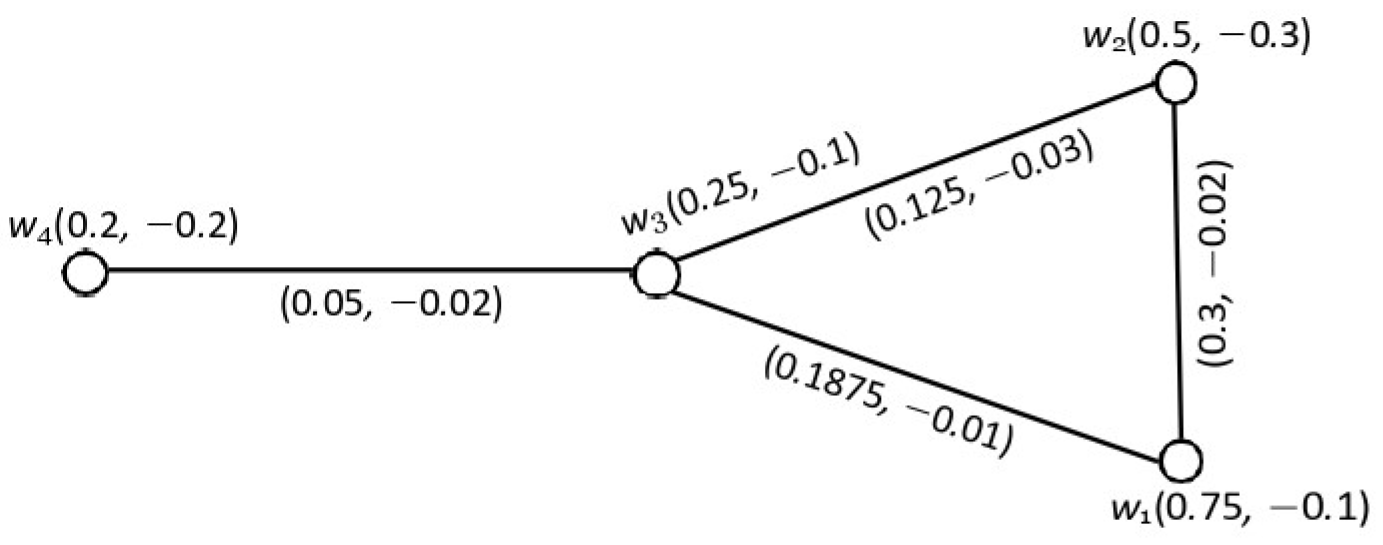
- 1.
- = , = , = , and =
- 2.
- = , = , = , and =
- 1.
- Let = = dominate , and dominate . So, by Definition 13, = is a DS of a graph
- 2.
- Let = = and and dominate , but neither nor dominate So, = is not a DS of a graph
- 3.
- Similarly, is a DS of a graph , but , , and are not DSs of a graph
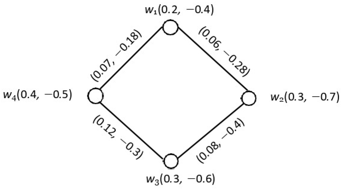
- 1.
- w does not dominate the elements in
- 2.
- There exists such that is the only element in that dominates
- Case (i) If , then does not dominate the elements in Suppose dominates the elements in . Then, is a DS of This is a contradiction, so no element in dominates w. Hence, property 1 holds.
- Case (ii) If then from above we know that Since is a DS of , then there exists such that dominates However, is not dominated by any element of Thus, therefore is the only element in that dominates Hence, property 2 holds.
- Suppose is not an MDS of Then, there exists a such that is a DS. Hence, w dominates the elements in Condition 1 does not hold.
- If is a DS, then for each element in , there exists an element in that dominates the elements in Condition 2 does not hold.
- 1.
- =
- 2.
- There is a vertex such that =
- If , then w is not dominated by any element in , which implies that =
- If , then is not dominated by any element in , but in , element only dominates Hence, = The converse is obvious. □
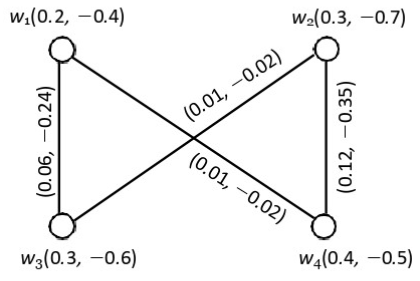
- 1.
- Let = and = , so = = and = = . Hence, the of is = min = .
- 2.
- The upper of a graph is = max = .
- 3.
- Furthermore, is the ⋎-set.
- If dominates , then dominates , where Hence, domination is a symmetric relation on
- If and for all then W is the only DS of
- = p if and only if and for all
- For any is precisely the set of all that are dominated by
4. Operations on Product Bipolar Fuzzy Graphs
4.1. Complement of a Product Bipolar Fuzzy Graph
- (i)
- = C.
- (ii)
- = for all
- (iii)
- = − and = −for all
- The complement of a complete graph is always a null graph.
- =
- If is a graph, then
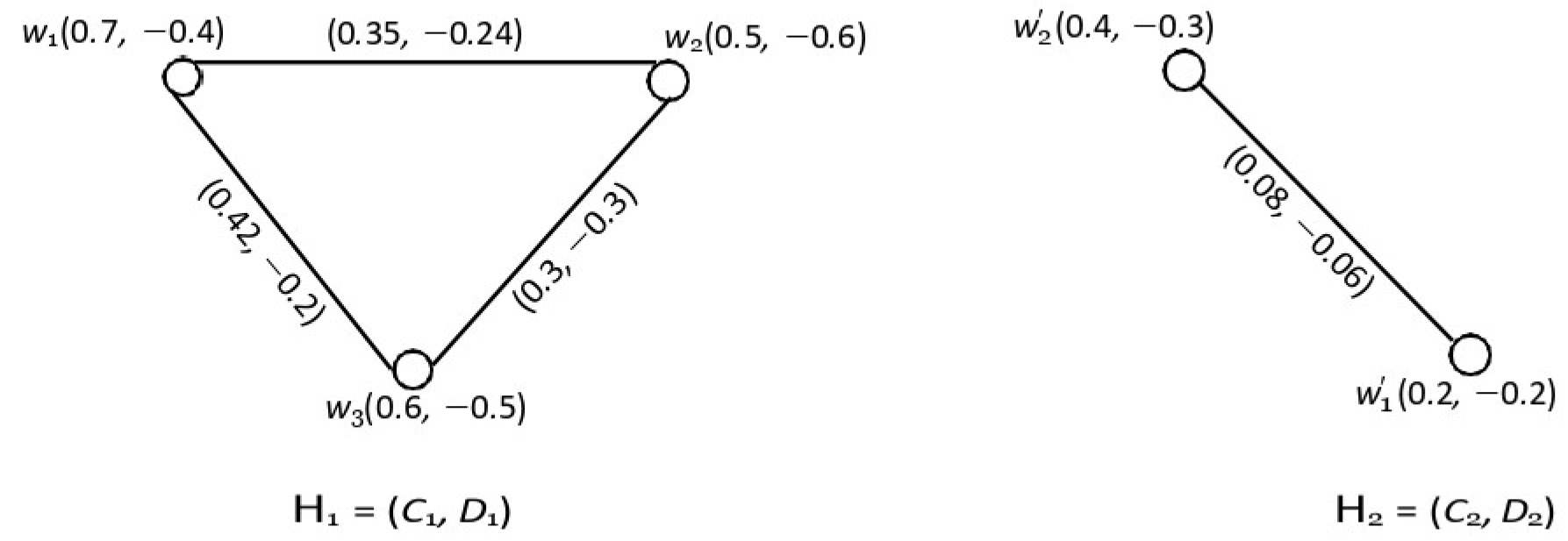
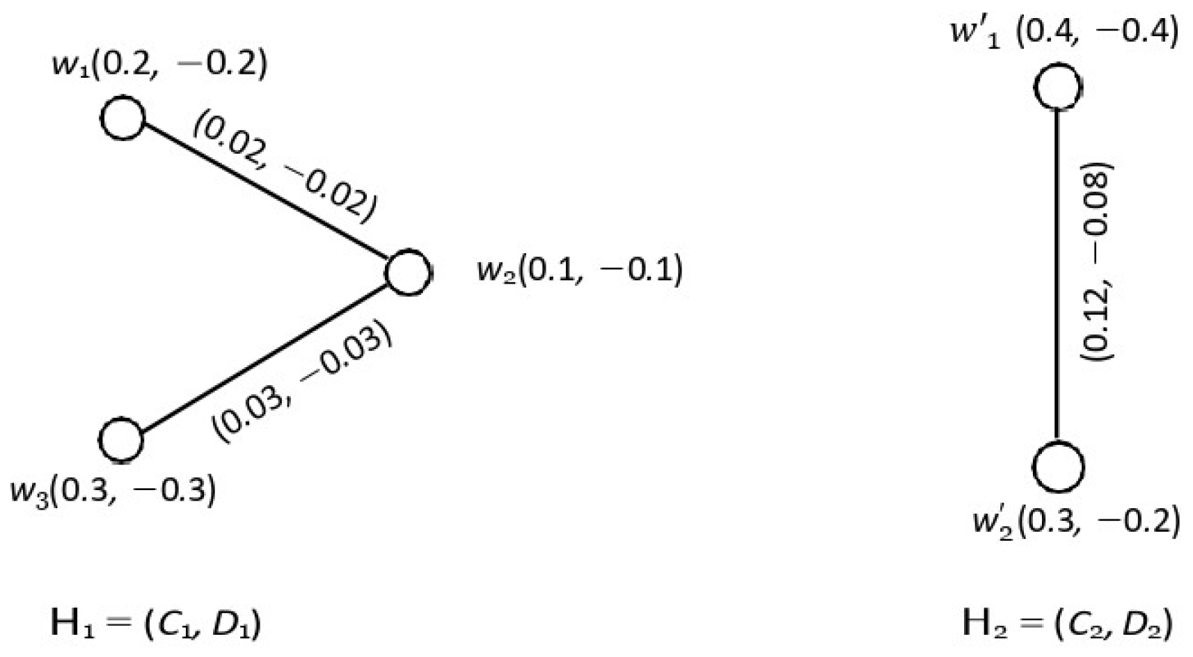
4.2. Union of Two Product Bipolar Fuzzy Graphs
- If , then there exists such that dominates
- If , then there exists such that dominates
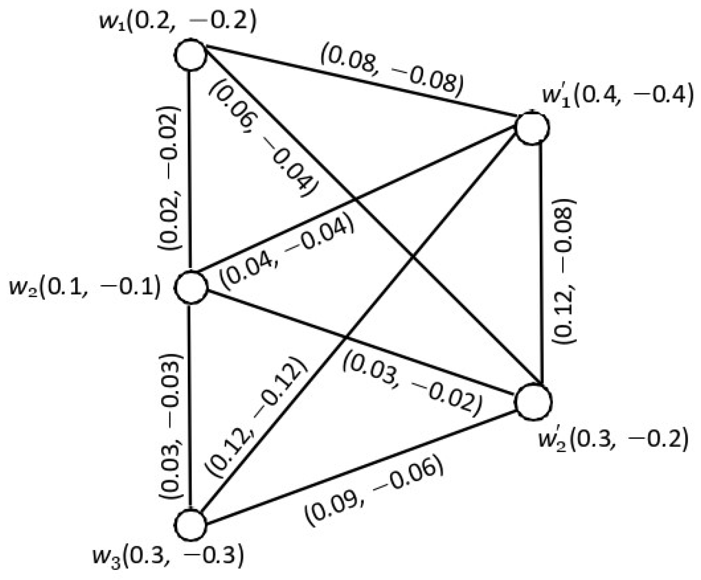
4.3. Joining Two Product Bipolar Fuzzy Graphs
- = , where is an MDS of
- = , where is an MDS of
- = , where , , and both and sets are not DSs of and , respectively.
4.4. Intersection of Two Product Bipolar Fuzzy Graphs
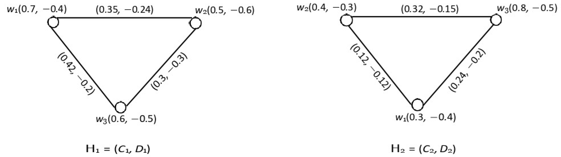
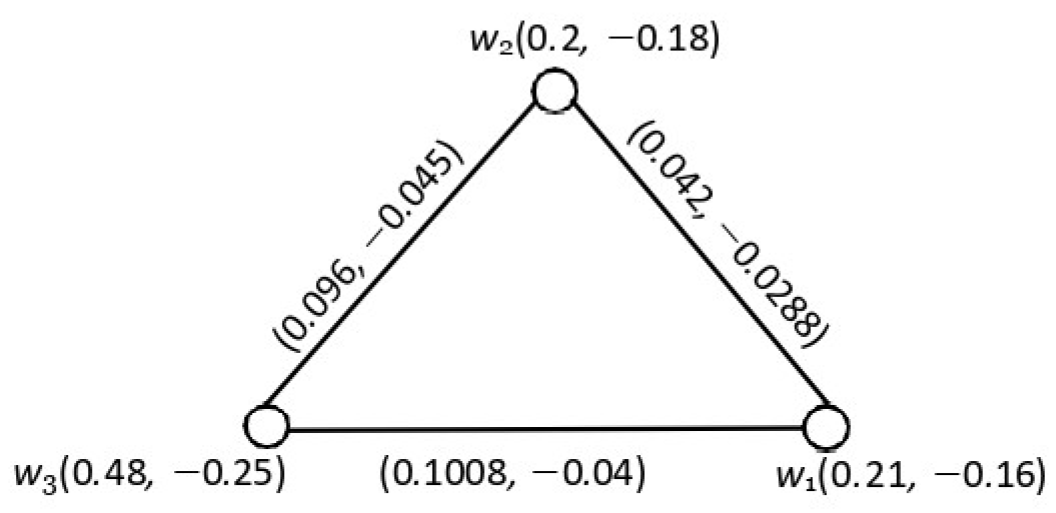
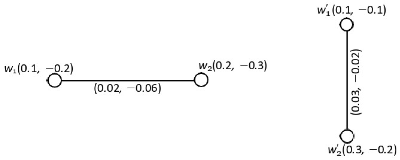
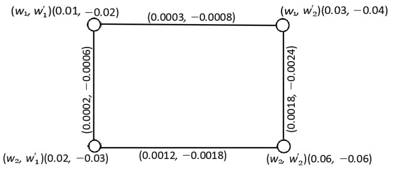
4.5. Cartesian Product of Two Product Bipolar Fuzzy Graphs
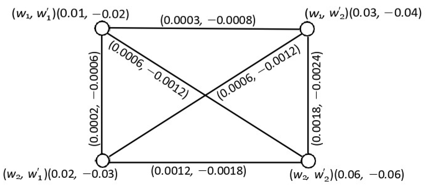
4.6. Composition of Two Product Bipolar Fuzzy Graphs
- Case (i) Suppose . Then,
- Case (ii) Suppose . Then,
- Case (iii) Suppose . Then,
- Case (i) Let and . Consider such that dominates w. Then,
- Case (ii) Let and . Consider such that dominates . Then,
- Case (iii) Let and . Consider and such that dominates w in and dominates in Then,
5. Relations Between Product Bipolar Fuzzy Graphs
- 1.
- and for all
- 2.
- and for all
- (i)
- = and = for all
- (ii)
- = and = for all
- (i)
- = and = for all
- (ii)
- = and = for all
6. Application of Domination in Product Bipolar Fuzzy Graph
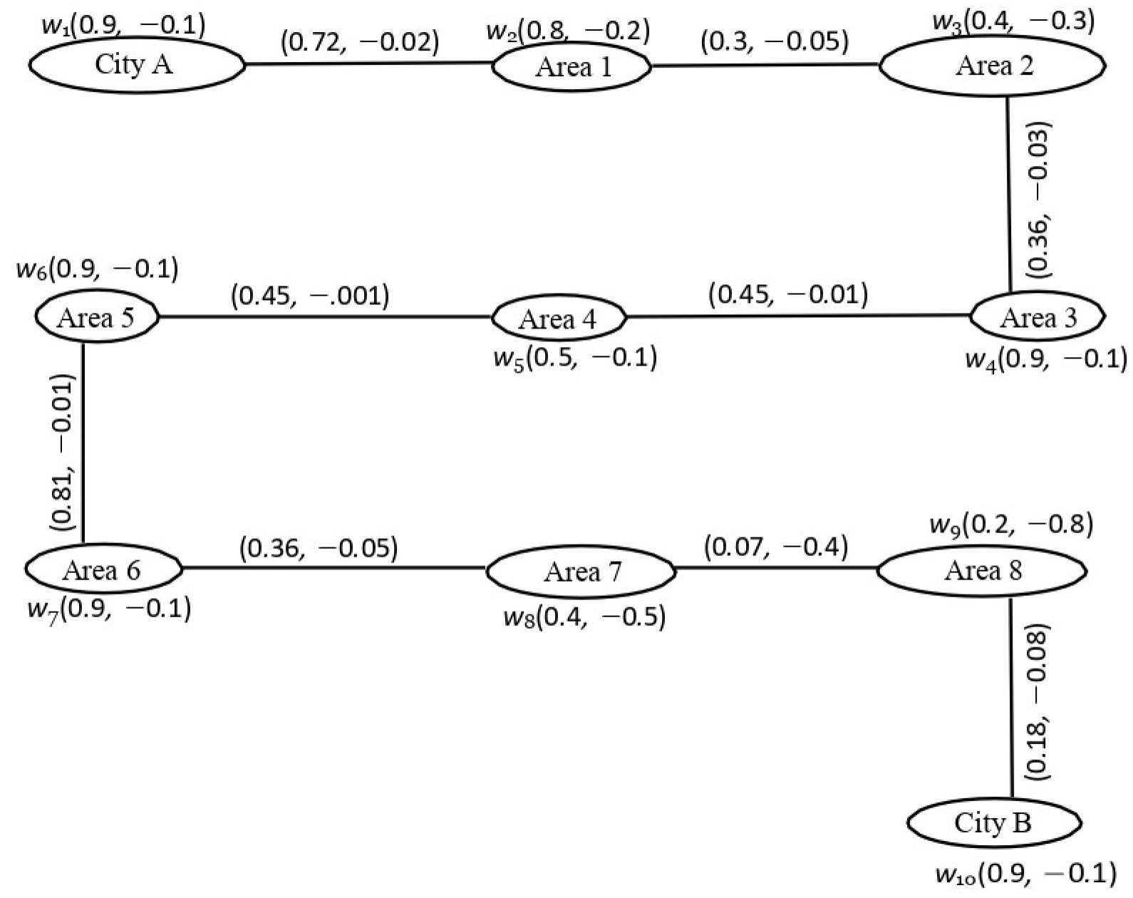
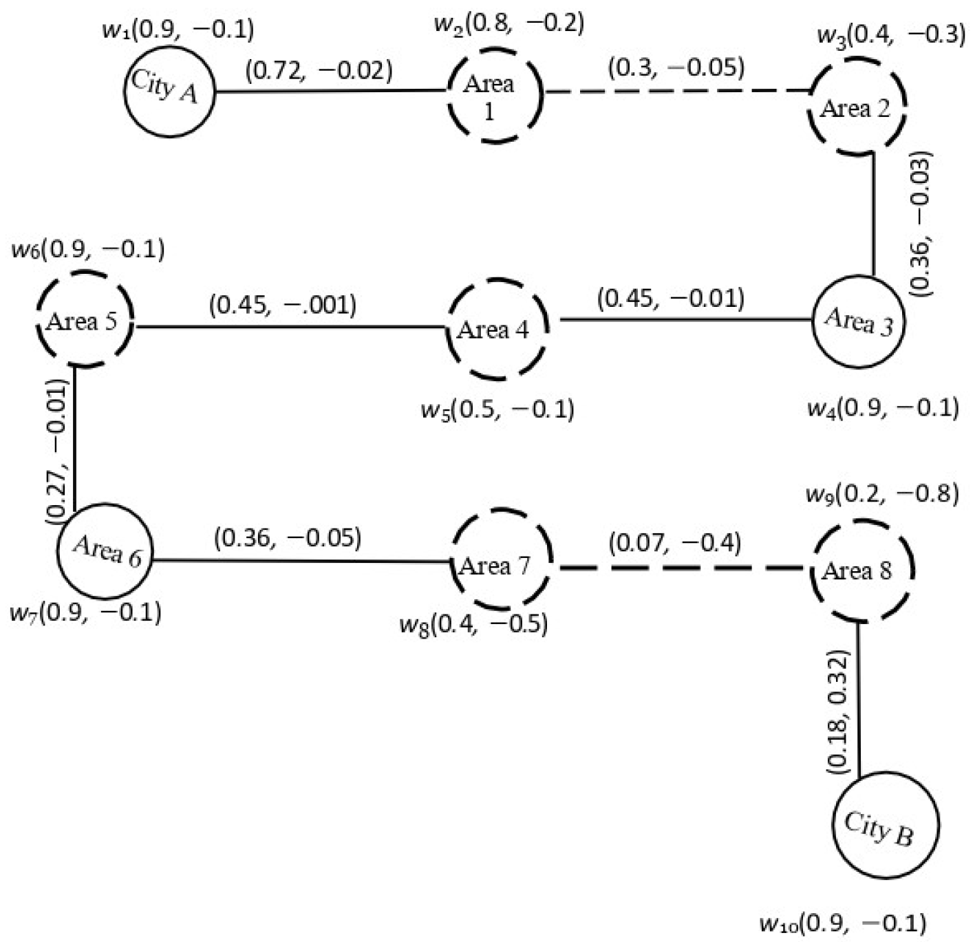
6.1. Locating Metro Bus Stations Using Domination
- The people who are living in Area 1 may use the nearby station in City A.
- The people who are living in Area 2 may use the nearby station in Area 3.
- The people who are living in Area 4 may use both nearby stations in Area 3 and Area 5.
- The people who are living in Area 7 may use the nearby station in Area 6.
- The people who are living in Area 8 may use the nearby station in City B.
| Algorithm 1: Method for Placing Stations of Metro Bus |
|
6.2. Comparison with Bipolar Fuzzy Graphs
- •
- If the membership grades of edges are less than equal to and greater than equal to the minimum and maximum of two vertices, respectively, we use the idea of domination on graphs.
- •
- In the case of the membership grades of edges being less than equal to and greater than equal to the product of two vertices, respectively, we use the theory of domination on graphs because in some cases, the theory of domination on graphs does not yield better results.
7. Conclusions and Future Directions
Author Contributions
Funding
Data Availability Statement
Acknowledgments
Conflicts of Interest
References
- Zadeh, L.A. Fuzzy sets. Inf. Control 1965, 8, 338–353. [Google Scholar]
- Zhang, W.R. Bipolar fuzzy sets and relations: A computational framework for cognitive modeling and multiagent decision analysis. In Proceedings of the First International Joint Conference of the North American Fuzzy Information Processing Society Biannual Conference, San Antonio, TX, USA, 18–21 December 1994; pp. 305–309. [Google Scholar]
- Zadeh, L.A. Similarity relations and fuzzy orderings. Inf. Sci. 1971, 3, 177–200. [Google Scholar]
- Kaufmann, A. Introduction à la Théorie des Ous-Ensembles Flous à L’usage des Ingénieurs (Fuzzy Sets Theory); Masson: Paris, France, 1975. [Google Scholar]
- Rosenfeld, A. Fuzzy graphs. In Fuzzy Sets and Their Applications to Cognitive and Decision Processes; Academic press: Cambridge, MA, USA, 1975; pp. 77–95. [Google Scholar]
- Bhattacharya, P. Some remarks on fuzzy graphs. Pattern Recognit. Lett. 1987, 6, 297–302. [Google Scholar]
- Mordeson, J.N.; Nair, P.S. Fuzzy Graphs and Fuzzy Hypergraphs; Physica: Amsterdam, The Netherlands, 2012; p. 46. [Google Scholar]
- Mordeson, J.N.; Chang-Shyh, P. Operations on fuzzy graphs. Inf. Sci. 1994, 79, 159–170. [Google Scholar]
- Sunitha, M.S.; Viiayakumar, A. Complement of a fuzzy graph. Indian J. Pure Appl. Math. 2002, 33, 1451–1464. [Google Scholar]
- Akram, M. Bipolar fuzzy graphs. Inf. Sci. 2011, 181, 5548–5564. [Google Scholar]
- Akram, M.; Shumaiza, A.J.C.R.; Alcantud, J.C.R. Multi-Criteria Decision Making Methods with Bipolar Fuzzy Sets; Springer: Singapore, 2023; Volume 2023, pp. 214–226. [Google Scholar]
- Ore, O. Theory of Graphs; American Mathematical Society Colloquium Publications: New York, NY, USA, 1962; Volume 38, pp. 206–212. [Google Scholar]
- Cockayne, E.J.; Hedetniemi, S.T. Towards a theory of domination in graphs. Networks 1977, 7, 247–261. [Google Scholar]
- Allan, R.B.; Laskar, R. On domination and independent domination of a graph. Discret. Math. 1978, 234, 73–76. [Google Scholar]
- Somasundaram, A.; Somasundarm, S. Domination in fuzzy graphs. Pattern Recognit. Lett. 1998, 19, 787–791. [Google Scholar]
- Karunambigai, M.G.; Akram, M.; Palanivel, K.; Sivasankar, S. Domination in bipolar fuzzy graphs. In Proceedings of the IEEE International Conference on Fuzzy Systems (FUZZ-IEEE), Hyderabad, India, 7–10 July 2013; pp. 1–6. [Google Scholar]
- Ponnappan, C.Y.; Ahamed, S.B.; Surulinathan, P. Edge domination in fuzzy graphs new approach. Int. J. IT Eng. Appl. Sci. Res. 2015, 4, 2319–4413. [Google Scholar]
- Ramaswamy, V.; Poornima, B. Product Fuzzy Graphs. IJCSNS Int. J. Comput. Sci. Netw. Secur. 2009, 9, 114–118. [Google Scholar]
- Shubatah, M.M. Domination in product fuzzy graphs. Adv. Comput. Math. Its Appl. 2012, 1, 119–125. [Google Scholar]
- Shubatah, M.M. Domination and Global Domination of Some Operations on Product Fuzzy Graphs. IJRDO-J. Math. 2020, 6, 41–53. [Google Scholar]
- Ahmed, H.; Alsharafi, M. Domination on bipolar fuzzy graph operations: Principles, proofs, and examples. Neutrosophic Syst. Appl. 2024, 17, 34–46. [Google Scholar]
- Gong, S.; Hua, G.; Gao, W. Domination of bipolar fuzzy graphs in various settings. Int. J. Comput. Intell. Syst. 2021, 14, 162. [Google Scholar]
- Akram, M.; Sarwar, M.; Dudek, W.A.; Akram, M.; Sarwar, M.; Dudek, W.A. Domination in Bipolar Fuzzy Graphs. In Graphs for the Analysis of Bipolar Fuzzy Information; Springer: Berlin/Heidelberg, Germany, 2021; pp. 253–280. [Google Scholar]
- Kalaiselvan, S.; Kumar, N.V.; Revathy, P. Inverse domination in bipolar fuzzy graphs. Mater. Today Proc. 2021, 47, 2071–2075. [Google Scholar]
- Mohamad, S.N.F.; Hasni, R.; Yusoff, B. On dominating energy in bipolar single–valued neutrosophic graph. Neutrosophic Sets Syst. 2023, 56, 10. [Google Scholar]
- Khan, W.A.; Taouti, A. Dominations in bipolar picture fuzzy graphs and social networks. Results Nonlinear Anal. 2023, 6, 60–74. [Google Scholar]
- Somasundaram, A. Domination in products of fuzzy graphs. Int. J. Uncertain. Fuzziness Knowl.-Based Syst. 2012, 13, 195–204. [Google Scholar]
- Akram, M.; Luqman, A. Fuzzy Hypergraphs and Related Extensions; Springer: Singapore, 2020. [Google Scholar]
- Mohanaselvi, V.; Sivamani, S. Paramount domination in bipolar fuzzy graphs. Int. J. Sci. Eng. Res. 2016, 7, 2229–5518. [Google Scholar]
- Ghorai, G.; Pal, M. Certain types of product bipolar fuzzy graphs. Int. J. Appl. Comput. Math. 2017, 3, 605–619. [Google Scholar]

| Abbreviations | Descriptions |
|---|---|
| graph | Product fuzzy graph |
| graph | Bipolar fuzzy graph |
| graph | Product bipolar fuzzy graph |
| DS | Dominating set |
| DSs | Dominating sets |
| MDS | Minimal dominating set |
| MDSs | Minimal dominating sets |
| Domination number |
| w | () | w | () |
|---|---|---|---|
| DSs | MDSs |
|---|---|
| , , | |
| , | |
| , | |
| , |
| w | () | w | () |
|---|---|---|---|
| w | () | w | () |
|---|---|---|---|
| w | () |
|---|---|
| w | () | w | () |
|---|---|---|---|
| w | () | w | () |
|---|---|---|---|
| () | () | () | () |
|---|---|---|---|
| W | Places | Positive Value | Negative Value |
|---|---|---|---|
| City A | |||
| Area 1 | |||
| Area 2 | |||
| Area 3 | |||
| Area 4 | |||
| Area 5 | |||
| Area 6 | |||
| Area 7 | |||
| Area 8 | |||
| City B |
| W | Places | Positive Value | Negative Value |
|---|---|---|---|
| (City A, Area 1) | |||
| (Area 1, Area 2) | |||
| (Area 2, Area 3) | |||
| (Area 3, Area 4) | |||
| (Area 4, Area 5) | |||
| (Area 5, Area 6) | |||
| (Area 6, Area 7) | |||
| (Area 7, Area 8) | |||
| (Area 8, City B) |
Disclaimer/Publisher’s Note: The statements, opinions and data contained in all publications are solely those of the individual author(s) and contributor(s) and not of MDPI and/or the editor(s). MDPI and/or the editor(s) disclaim responsibility for any injury to people or property resulting from any ideas, methods, instructions or products referred to in the content. |
© 2025 by the authors. Licensee MDPI, Basel, Switzerland. This article is an open access article distributed under the terms and conditions of the Creative Commons Attribution (CC BY) license (https://creativecommons.org/licenses/by/4.0/).
Share and Cite
Ming, W.; Rasool, A.; Ishtiaq, U.; Shahzadi, S.; Garayev, M.; Popa, I.-L. Optimizing Decision-Making Using Domination Theory in Product Bipolar Fuzzy Graphs. Symmetry 2025, 17, 479. https://doi.org/10.3390/sym17040479
Ming W, Rasool A, Ishtiaq U, Shahzadi S, Garayev M, Popa I-L. Optimizing Decision-Making Using Domination Theory in Product Bipolar Fuzzy Graphs. Symmetry. 2025; 17(4):479. https://doi.org/10.3390/sym17040479
Chicago/Turabian StyleMing, Wei, Areen Rasool, Umar Ishtiaq, Sundas Shahzadi, Mubariz Garayev, and Ioan-Lucian Popa. 2025. "Optimizing Decision-Making Using Domination Theory in Product Bipolar Fuzzy Graphs" Symmetry 17, no. 4: 479. https://doi.org/10.3390/sym17040479
APA StyleMing, W., Rasool, A., Ishtiaq, U., Shahzadi, S., Garayev, M., & Popa, I.-L. (2025). Optimizing Decision-Making Using Domination Theory in Product Bipolar Fuzzy Graphs. Symmetry, 17(4), 479. https://doi.org/10.3390/sym17040479