Efficient Coastal Mangrove Species Recognition Using Multi-Scale Features Enhanced by Multi-Head Attention

Abstract

Recognizing mangrove species is a challenging task in coastal wetland ecological monitoring due to the complex environment, high species similarity, and the inherent symmetry within the structural features of mangrove species. Many species coexist, exhibiting only subtle differences in leaf shape and color, which increases the risk of misclassification. Additionally, mangroves grow in intertidal environments with varying light conditions and surface reflections, further complicating feature extraction. Small species are particularly hard to distinguish in dense vegetation due to their symmetrical features that are difficult to differentiate at the pixel level. While hyperspectral imaging offers some advantages in species recognition, its high equipment costs and data acquisition complexity limit its practical application. To address these challenges, we propose MHAGFNet, a segmentation-based mangrove species recognition network. The network utilizes easily accessible RGB remote sensing images captured by drones, ensuring efficient data collection. MHAGFNet integrates a Multi-Scale Feature Fusion Module (MSFFM) and a Multi-Head Attention Guide Module (MHAGM), which enhance species recognition by improving feature capture across scales and integrating both global and local details. In this study, we also introduce MSIDBG, a dataset created using high-resolution UAV images from the Shankou Mangrove National Nature Reserve in Beihai, China. Extensive experiments demonstrate that MHAGFNet significantly improves accuracy and robustness in mangrove species recognition.

1. Introduction

Mangroves are vital coastal ecosystems that provide significant ecological, economic, and social benefits [1,2,3]. Extensively distributed across tropical and subtropical regions, they serve as natural coastal barriers, reducing erosion, buffering storm surges, and mitigating climate change impacts by sequestering large amounts of carbon [4,5]. Additionally, mangroves support diverse biodiversity, functioning as nurseries for marine species and habitats for various birds and wildlife [6].

However, over the past few decades, mangroves have faced increasingly severe threats from global climate change, rising sea levels, coastal development, and human activities. These pressures have resulted in a continuous decline in mangrove coverage, habitat fragmentation, and the degradation of ecological functions, with some species even at risk of extinction [7,8]. Consequently, the protection and monitoring of mangrove ecosystems—particularly through species identification and ecological assessment—have become critical from both scientific and practical perspectives [9].

Mangrove species recognition has long been a challenging task due to the significant morphological similarity between species [10] and their frequent co-existence within the same environment. Distinguishing species accurately using the naked eye or traditional measurement methods is inherently difficult. Furthermore, variations in growth stages, external morphology, and canopy structure add to the complexity of species identification [11].

Moreover, mangroves exhibit high species diversity, spatiotemporal heterogeneity, and intricate community structures [12,13]. These factors pose significant challenges to mangrove conservation and research, especially in large-scale ecological monitoring. The inability to accurately classify species directly affects assessments of mangrove health and species distribution.

With the rapid advancement of UAV and spectral technologies, traditional mangrove species classification has increasingly leveraged hyperspectral and multispectral data. For example, Cao [14] utilized UAV hyperspectral images to classify mangrove species on Qi’ao Island, Zhuhai, Guangdong Province, China. By integrating spectral, textural, and height features and applying SVM, the study achieved an accuracy of 88.66%, demonstrating the effectiveness of UAV hyperspectral data in species recognition. Similarly, Zulfa [15] applied the SAM spectral algorithm to classify mangrove species in the Matang Mangrove Forest Reserve (MMFR). The study employed SID and SAM algorithms to classify 40,000 trees from 19 mangrove species using medium-resolution satellite images. The SAM algorithm achieved a classification accuracy of 85.21%, and the findings indicated that mangrove species distribution was influenced by human activities. Both algorithms demonstrated complementary strengths in enhancing mangrove species identification.

Wang [16] employed the Extremely Randomized Trees (ERT) algorithm with multi-source remote sensing data to classify mangrove species in Fucheng Town, Leizhou City. By combining optical data (Gaofen-1, Sentinel-2, Landsat-9) and fully polarized SAR data (Gaofen-3), the study achieved a high classification accuracy of 90.13% (Kappa = 0.84). The ERT algorithm outperformed other methods, such as Random Forest and K-Nearest Neighbors (KNN), demonstrating the effectiveness of multi-source and multi-temporal satellite data for mangrove species classification.

Cao [17] combined UAV-based hyperspectral and LiDAR data for fine mangrove species classification in Qi’ao Island, Zhuhai, China. The proposed method, which used the Rotation Forest (RoF) algorithm, achieved an overall accuracy of 97.22%, outperforming other algorithms, such as Random Forest (RF) and Logistic Model Tree (LMT). Incorporating LiDAR-derived canopy height improved classification accuracy by 2.43%.

Zhen [18] utilized the XGBoost algorithm with multi-source satellite remote sensing data to classify mangrove species. By integrating data from WorldView-2, Orbita HyperSpectral, and ALOS-2, they achieved a high classification accuracy of 94.02% for six mangrove species. This study highlights the value of combining spectral, texture, and polarization features to improve mangrove species mapping and support conservation efforts.

Meanwhile, Yang [19] compared the performance of four machine learning algorithms—Adaptive Boosting (AdaBoost), eXtreme Gradient Boosting (XGBoost), Random Forest (RF), and Light Gradient Boosting Machine (LightGBM)—for classifying mangrove species using both multispectral and hyperspectral data. The study found that the average recognition accuracy for multispectral data was 72%, while hyperspectral data achieved an average accuracy of 91%. The highest accuracy, 97.15%, was achieved using the LightGBM method.

Although hyperspectral data offer a high resolution and the ability to capture subtle species differences, with strong robustness in complex environments, obtaining high-quality hyperspectral data presents numerous challenges. Variations in lighting, terrain, and occlusions in complex environments like wetlands can significantly affect data quality. Additionally, hyperspectral sensors are expensive, with high hardware and maintenance costs, which limits their widespread application in large-scale or long-term monitoring.

In recent years, significant progress has been made in the segmentation of UAV remote sensing images. With the development of deep learning [20], semantic segmentation networks have achieved remarkable advancements. However, the potential of these networks for mangrove species recognition remains largely unexplored. The Fully Convolutional Network (FCN) [21] was one of the earliest networks applied to semantic segmentation. It replaces fully connected layers with convolutional layers for end-to-end image segmentation. While FCN is simple and efficient, its performance is limited in complex scenarios, particularly when distinguishing subtle differences among mangrove species.

DeepLab v3 [22] and DeepLab v3+ [23] introduced atrous convolution and the Atrous Spatial Pyramid Pooling (ASPP) technique. These improvements significantly enhance segmentation accuracy, especially in capturing multi-scale information. However, these models still struggle to process fine-grained details, especially when it comes to capturing subtle edges and leaf structures, particularly in mangrove images.

UperNet [24] enhances segmentation by combining global context and local details. However, it struggles with small-scale features, which impacts recognition accuracy. MobileNet [25] is a lightweight network designed for mobile devices. It offers efficient computational performance, but it faces difficulties in capturing both global and local details in complex mangrove environments, which results in a decline in segmentation and recognition performance.

OCRNet [26] improves context expression through its object context module. This enhances overall scene understanding. However, OCRNet performs poorly under complex lighting conditions, with accuracy dropping under strong light and shadow. DMNet [27] (Dynamic Multi-scale Network) improves model flexibility by adjusting feature representations at different scales. However, it still fails to capture fine details of leaves and canopy structures in mangroves.

Although networks like Swin Transformer [28] capture global information effectively, they still encounter challenges when handling subtle species differences and complex backgrounds in mangrove environments.

To address the shortcomings of existing methods in mangrove species recognition, this paper proposes a segmentation network named MHAGFNet, based on UAV remote sensing images, aimed at significantly improving the recognition accuracy of mangrove species through image segmentation techniques. The experimental results demonstrate that the proposed MHAGFNet achieves an average recognition accuracy of 93.87% for five mangrove species on the constructed dataset, with an average segmentation accuracy of 88.46%, demonstrating excellent performance.

The main contributions of this paper are as follows:

1. Design of the Multi-Scale Feature Fusion Module (MSFFM): MSFFM combines early shallow features, such as detailed texture information, with deep features, such as high-level semantic information, to enhance the ability to distinguish visually similar mangrove species.

2. Design of the Multi-Head Attention Guide Module (MHAGM): MHAGM captures multi-scale features from the images, improving the proposed MHAGFNet’s ability to perceive both global structures and fine details.

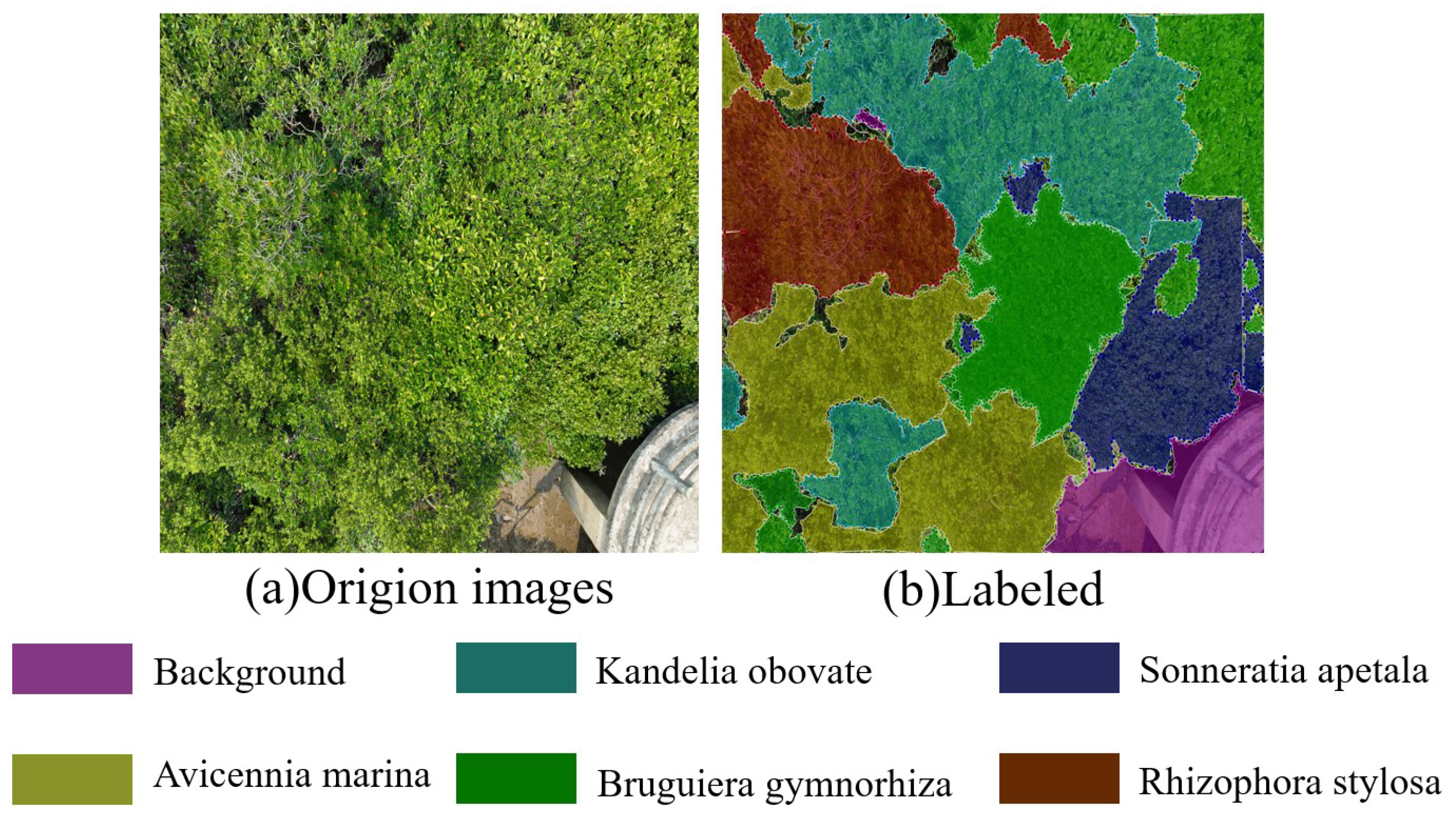
3. Building a Mangrove species dataset (MSIDBG) using a high-resolution UAV: This MSIDBG dataset was collected in Shankou Mangrove National Nature Reserve in Beihai, Guangxi Zhuang Autonomous Region, China, and serves as an important basic resource for mangrove species recognition research.

2. Mangrove Species Selection and Challenges

Mangroves grow in the intertidal zones of tropical and subtropical coastal areas, playing important roles such as purifying seawater, breaking waves, sequestering carbon, and maintaining biodiversity.

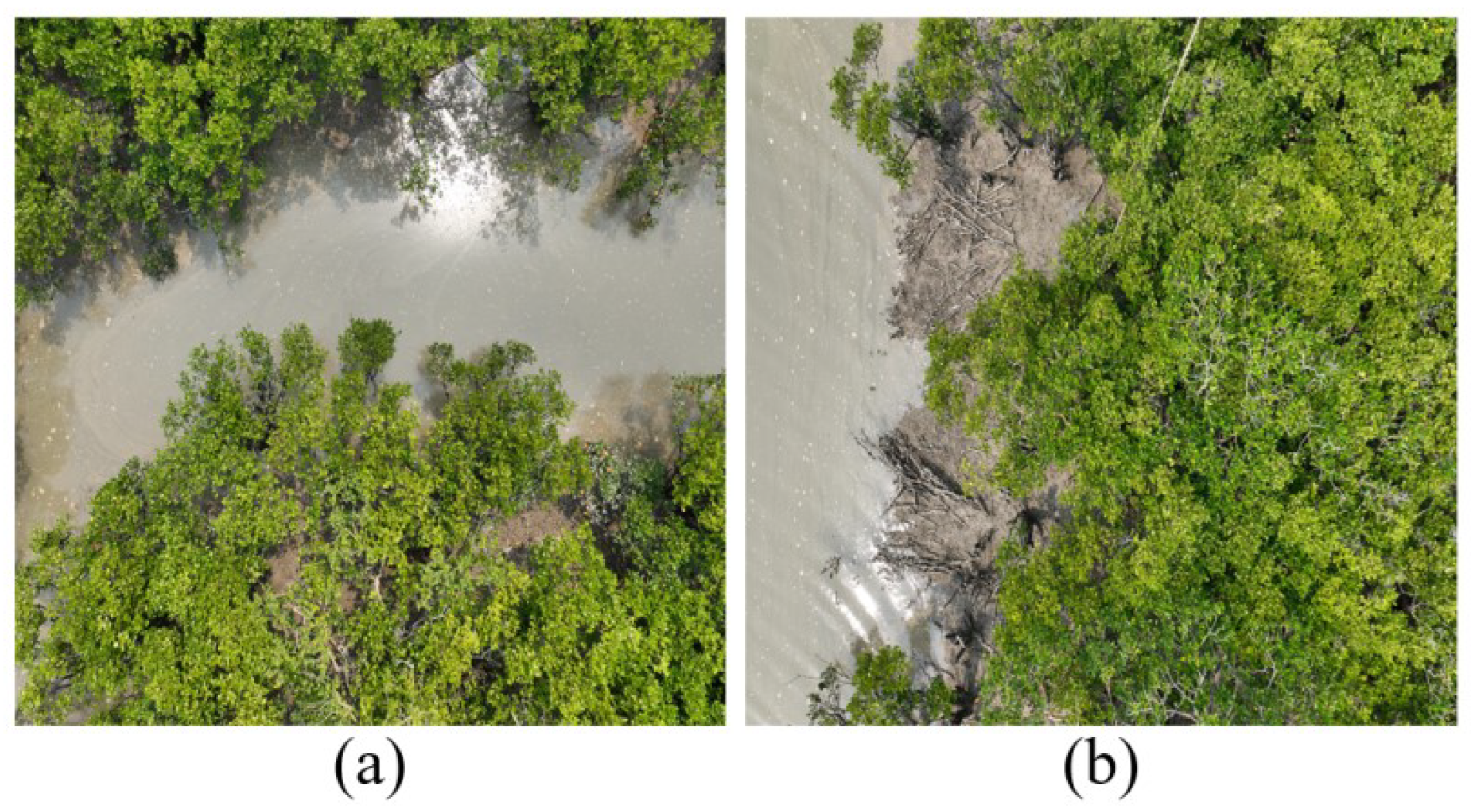
Mangrove species typically grow in similar intertidal environments, as shown in Figure 1a,b. The similarity in background height makes it challenging to distinguish them based solely on environmental features. Additionally, variations in light angles, shadow effects, and strong reflections can affect image clarity and detail capture, increasing the complexity of image processing and species recognition.

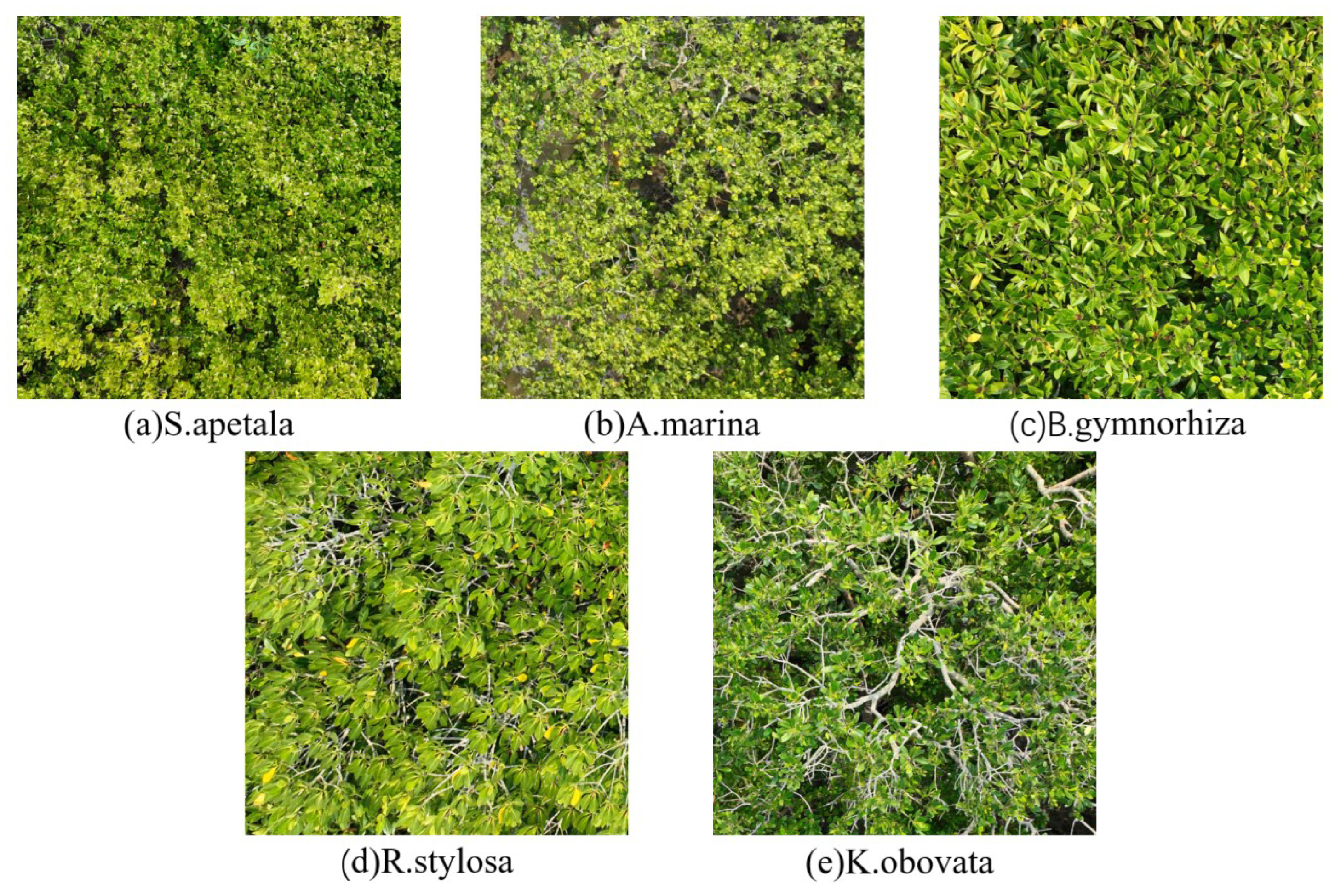
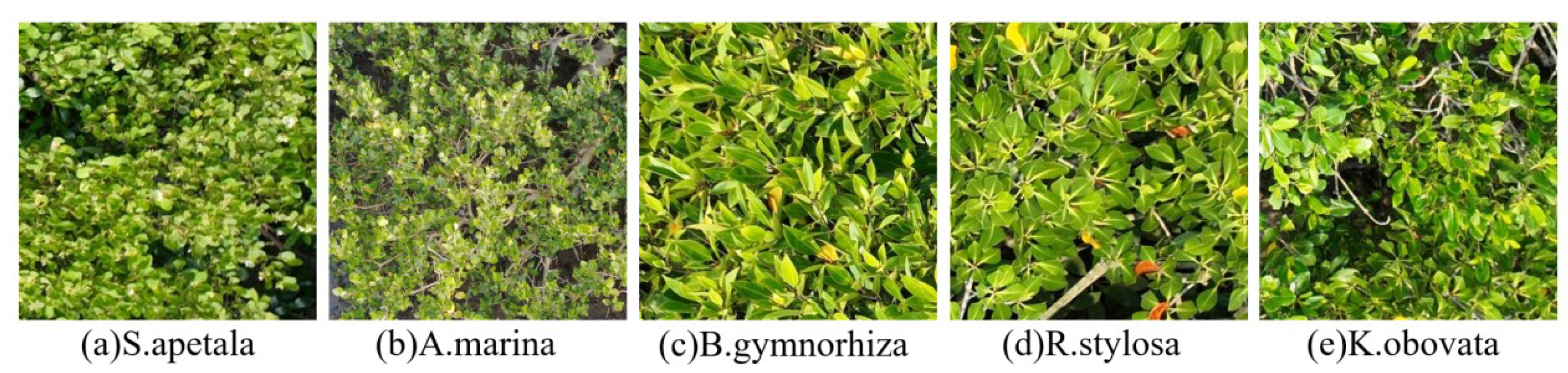
The mangrove ecosystem in southern China, as shown in Figure 2. Figure 2a–e display the following species: (a) Sonneratia apetala, (b) Avicennia marina, (c) Bruguiera gymnorhiza, (d) Rhizophora stylosa and (e) Kandelia obovata.

Figure 2a: Sonneratia apetala, an exotic mangrove species native to the Bay of Bengal and the Indochina region. Its leaves are oval-shaped, and its fruits are green and round. Sonneratia apetala adapts to humid and low-oxygen environments, often growing in mudflats and intertidal zones. However, due to its common leaf morphology and partial similarity with other species, combined with its relatively short stature and susceptibility to tidal influences (mud coverage), recognition in complex environments can be challenging.

Figure 2b: Avicennia marina, a highly salt-tolerant mangrove species that thrives in environments with high salinity and frequent tidal inundation. Its leaves are thick with a waxy surface, and its bark is grayish-white. This species exhibits remarkable adaptability to extreme environments; however, its bark color and leaf morphology can resemble those of some terrestrial plants, leading to potential misclassification in the complex mangrove growth environment.

Figure 2c: Bruguiera gymnorhiza, with smooth, dark green leaves and slight serrations along the edges. These leaf characteristics aid its growth in the intertidal zone. However, in dense mangrove areas, the leaves of Bruguiera gymnorhiza may be confused with those of Rhizophora stylosa, complicating recognition.

Figure 2d: Rhizophora stylosa, characterized by opposite leaves with blunt tips, which are typically larger and dark green, exhibiting strong adaptability. Although the leaf morphology of Rhizophora stylosa is relatively distinctive, in certain situations, variations in shadow and light may affect recognition, leading to blurred boundaries.

Figure 2e: Kandelia obovata, with smooth, oval-shaped leaves with serrated edges, and elongated seeds. The leaves are highly adaptable and can survive in saline-alkaline environments. While its morphology is relatively easy to identify, similarities with the leaves of Sonneratia apetala in certain features may pose recognition challenges in dense mangrove areas.

As can be seen from Figure 2, mangrove species recognition faces several challenges, with the first being the morphological similarity between species. Although each species differs in leaf shape and fruit morphology, these visual differences can become blurred in images captured from a distance or with a lower resolution. For instance, as shown in Figure 2, the leaves of Sonneratia apetala and Avicennia marina are easily confused under varying conditions, as their leaf colors and shapes appear similar. This similarity in morphological features exhibits a form of symmetry that challenges the recognition model to differentiate species accurately. Similarly, distinguishing the leaves of Bruguiera gymnorhiza and Rhizophora stylosa in Figure 2 may be difficult under changing light conditions or shadows.

3. Methods

In this section, we first introduce the overall network architecture. Then, we provide a detailed description of each submodule.

3.1. Overview of the Architecture

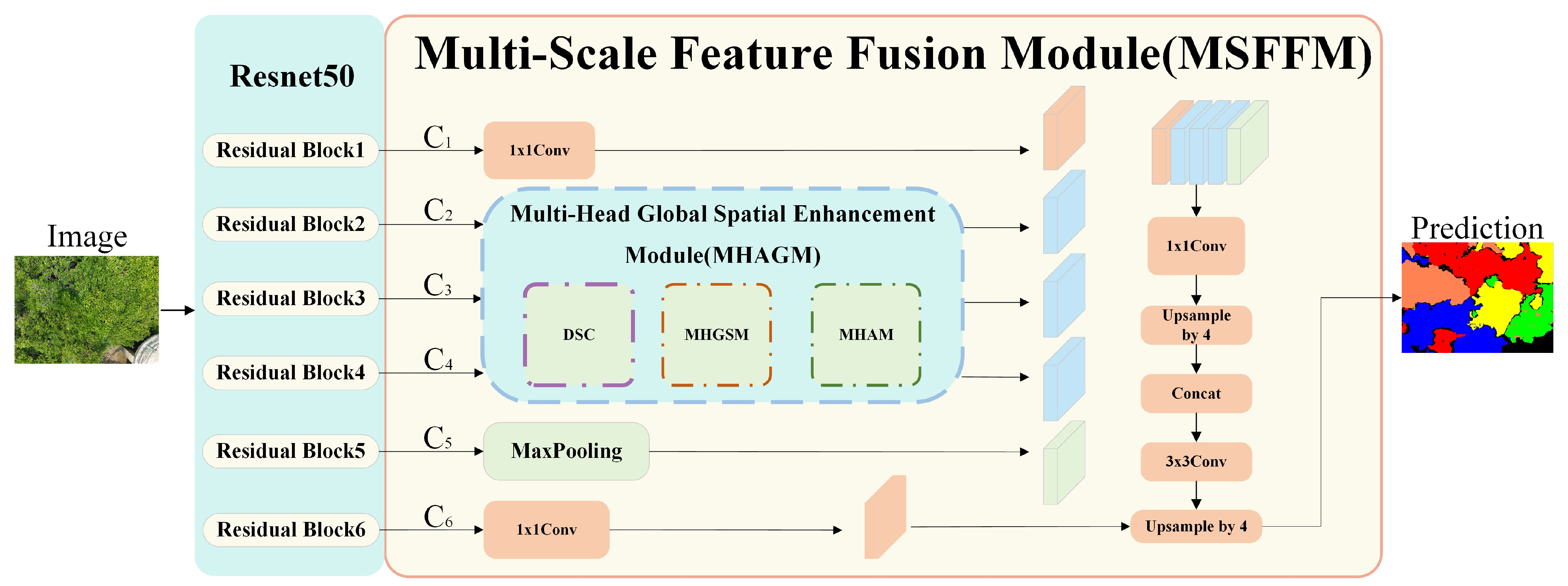
The overall architecture of the proposed MHAGFNet is shown in Figure 3. MHAGFNet consists of the ResNet50 [29] backbone network and the Multi-Scale Feature Fusion Module (MSFFM). ResNet50, as the backbone network for feature extraction, generates six feature maps of different resolutions from the input images. These feature maps represent information from low-level to high-level features, providing a rich feature base for subsequent modules. The Multi-Scale Feature Fusion Module (MSFFM) mainly includes the Multi-Head Attention Guide Module (MHAGM). By enhancing feature maps at different levels through multi-head attention guidance, MSFFM can better extract and fuse features from various scales, thereby improving the network’s ability to recognize mangrove species, particularly in situations with complex backgrounds and varying lighting conditions.

3.2. Multi-Scale Feature Fusion Module (MSFFM)

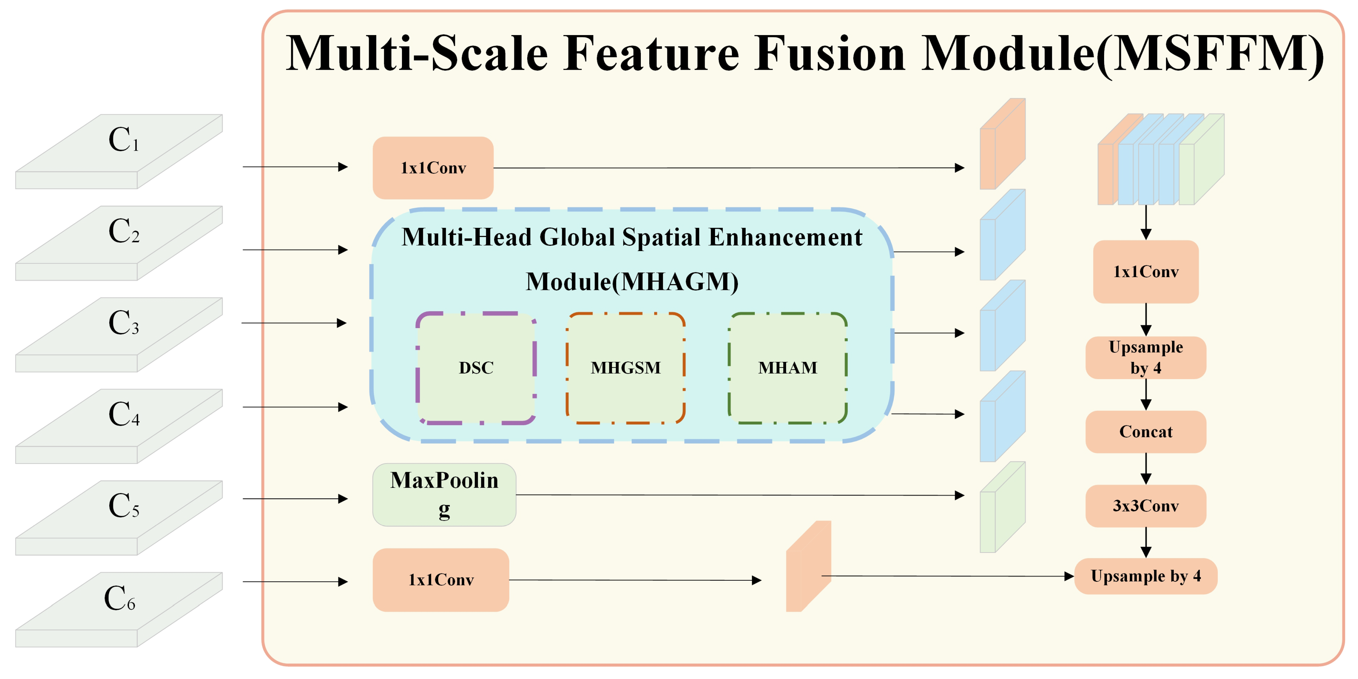
Here, we provide a detailed explanation of the core module, the MSFFM module in MHAGFNet. The structure of MSFFM is shown in Figure 4, which comprises a 1 × 1 convolution layer, three Multi-Head Attention Guide Modules (MHAGM), a feature fusion layer, an upsampling layer, and a transposed convolution layer.

MHAGM is the core component of MSFFM, consisting of three key submodules: Depthwise Separable Convolution, Multi-Head Global Spatial Enhancement Module (MHGSEM), and Mangrove All-View Attention Module (MHAM). It captures key information across different scales through the multi-head attention mechanism, enhancing the model’s sensitivity to the features of various mangrove species. Each MHAGM module independently processes features at different scales, ensuring that the model can effectively handle the complex and variable environments of mangroves and capture subtle feature differences. The feature fusion layer efficiently integrates features from various scales, reinforcing the synergy between local and global information, thereby enhancing recognition performance. The upsampling layer and transposed convolution layer restore the spatial resolution of the feature maps, ensuring that the final output segmentation results achieve higher precision. Through the extraction and fusion of multi-scale features, the MSFFM significantly improves the accuracy of mangrove species recognition in complex backgrounds and changing environments. In addition, the 1 × 1 convolution layer is utilized to reduce the channel dimensions and perform preliminary processing on the input features, preserving important information while minimizing computational complexity.

The flow of MSFFM starts with a 1 × 1 convolution applied to feature map C1, resulting in feature map F1, which reduces computational complexity. Next, feature maps C2 to C4 are input into the MHAGM modules, where they are processed using the multi-head attention mechanism, yielding enhanced feature maps F2, F3, and F4. Feature maps C5 and C6 are then processed with max pooling and 1 × 1 convolution operations, respectively, producing feature maps F5 and F6. Subsequently, feature maps F1 through F5 are fused together, followed by further compression of the fused features using a 1 × 1 convolution. This is followed by a 4× upsampling operation to enhance the resolution while retaining more detailed information. The upsampled features are concatenated with the compressed feature map F6, integrating features from all levels. Finally, the fused features undergo further processing through a 3 × 3 convolution, and a transposed convolution generates the final segmentation map. The transposed convolution restores spatial resolution and ensures the accuracy of the segmentation results.

3.3. Multi-Head Attention Guide Module (MHAGM)

Here, we provide a detailed explanation of MHAGM in MSFFM, as shown in Figure 4. The structure of MHAGM is illustrated in Figure 5. It consists of Depthwise Separable Convolution (DSC), the Multi-Head Global and Spatial Enhanced Module (MHGSEM), the Multi-Head Attention Module (MHAM), and skip connections.

Depthwise Separable Convolution (DSC) extracts local features from input data by expanding the convolution kernel and applying dilation rates, thereby enhancing feature extraction efficiency. This improves performance in complex mangrove environments.

The MHGSEM combines multi-head channel attention and spatial attention mechanisms. It enhances feature representation at both global and local levels, thereby improving the network’s recognition accuracy in complex backgrounds.

The MHAM module enhances the network’s ability to capture subtle mangrove feature differences. It integrates global, local, and edge features through a multi-dimensional attention mechanism.

Batch normalization and the ReLU activation function help accelerate model convergence. They also improve the ability to capture non-linear feature representations, enhancing overall performance.

(1) DSC Module

The MHAGM module first decomposes the Depthwise Separable Convolution (DSC) into a depthwise convolution and a pointwise convolution. The depthwise convolution extracts spatial features independently for each channel, while the pointwise convolution aggregates information across channels. Compared to standard convolution, depthwise separable convolution significantly reduces computational complexity. For an input feature map $x\in {\mathbf{R}}^{B\times C\times H\times W}$, its computational process is as follows:

$$x_d={\mathrm{Conv}}_{\mathrm{d}}(x,W_{\mathrm{d}})$$

(1)

$$x_{\mathrm{p}}={\mathrm{Conv}}_{\mathrm{p}}(x_{\mathrm{d}},W_{\mathrm{p}})$$

(2)

where $Con{v}_{\mathrm{d}}$ represents the operation using a 3 × 3 convolutional kernel applied independently to each channel, while $Con{v}_{\mathrm{p}}$ denotes the operation using a 1 × 1 convolutional kernel to perform a linear transformation on the channel dimension.

(2) MHGSEM Module

The feature map is then fed into the MHGSEM module, which adaptively adjusts the importance of each channel. MHGSEM extracts global information using a multi-head attention mechanism and generates weights to modulate each channel’s contribution. After learning the weights for different channels, they are normalized using the Sigmoid function to obtain the enhanced features. The formula is as follows:

$$x_{\mathrm{MH}}=x\times \sigma \left(\mathrm{MHGSEM}\left(x\right)\right)$$

(3)

where $\sigma$ represents the Sigmoid function.

(3) MHAM Module

After obtaining the enhanced features, to better focus on the edges, shapes, and textures of the mangrove leaves, they are fed into the MHAM module to further capture important spatial information. The formula is as follows:

$$x_{\mathrm{HA}}=x\times \sigma \left(\mathrm{MHAM}\left(x_{\mathrm{MH}}\right)\right)$$

(4)

(4) Residual connection

Finally, to mitigate the vanishing gradient problem and accelerate convergence, a skip connection is used to enhance the propagation of residual information. When the input and output channels differ, the skip connection adjusts the dimensions using a 1 × 1 convolution and adds it to the feature map after convolution, thereby maintaining the integrity of the features. The formula is as follows:

$$y=\mathrm{ReLU}(x_{\mathrm{HA}}\times x+\mathrm{Shortcut}\left(x\right))$$

(5)

where $\mathrm{Shortcut}(·)$ represents the skip connection, and $\mathrm{ReLU}(·)$ represents the activation function.

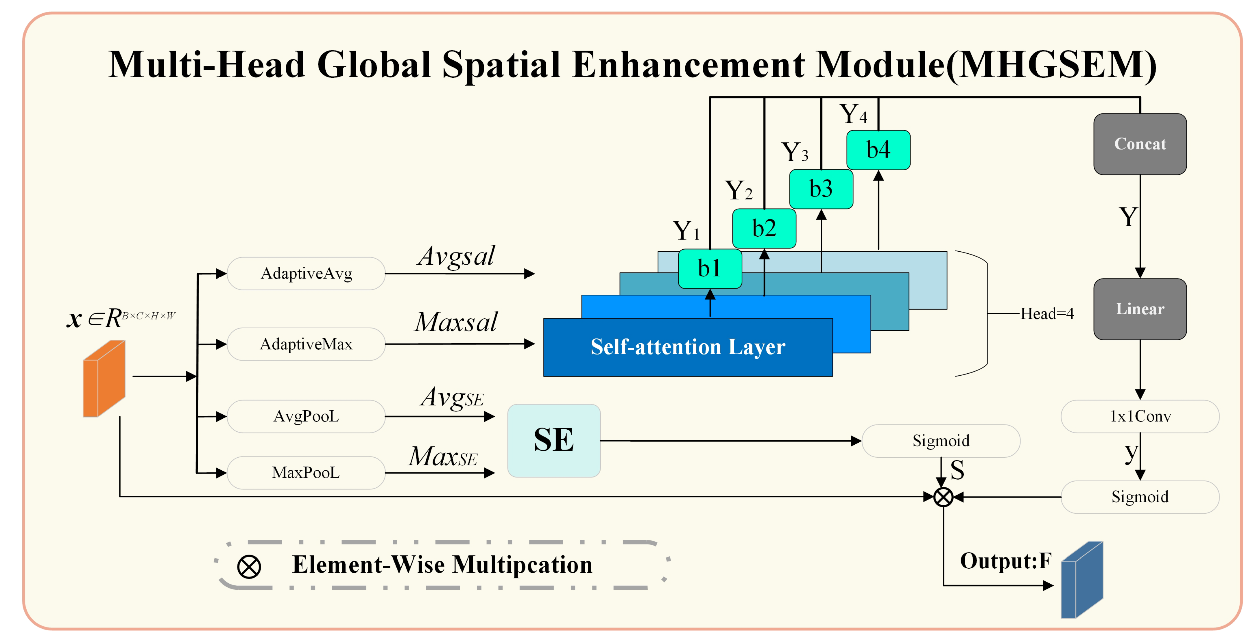
3.4. Multi-Head Global Spatial Enhancement Module (MHGSEM)

Here, we provide a detailed explanation of the MHGSEM in the MHAGM, as shown in Figure 5. The structure of MHGSEM is illustrated in Figure 6. It consists of a multi-head self-attention mechanism, a spatial attention module, and a feature fusion module.

The multi-head self-attention fully connected layer computes relationships between channels using a multi-head mechanism. Each attention head focuses on different aspects of the feature map, improving the performance of the channel attention mechanism.

The spatial attention module enhances spatial feature extraction across the feature map. It emphasizes key spatial information, such as mangrove boundaries and textures, which aids in the recognition of small mangrove species in complex scenes with lighting variations and water reflections.

The feature fusion module combines channel and spatial attention, ensuring the fused feature map retains both global and local details. This integration strengthens the model’s ability to capture comprehensive feature representations at multiple scales.

(1) Multi-head fully connected layer

For the input feature map $x\in {\mathbf{R}}^{B\times C\times H\times W}$, both adaptive global average pooling and adaptive global max pooling are applied simultaneously to reduce the dimensionality of the input features. This step extracts channel-level global features ${Avg}_{sal}$ and ${Max}_{sal}$. The resulting global features are then passed into the multi-head attention mechanism. In this mechanism, the outputs of the average pooling and max pooling are processed separately by four fully connected layers. The output of each head is represented as:

$$Y_i={\mathrm{FC}}_i\left(\mathrm{AvgPool}\left(x\right)\right)+{\mathrm{FC}}_i\left(\mathrm{MaxPool}\left(x\right)\right)$$

(6)

where $Y_i$ represents different attention heads, and ${FC}_i$ is the fully connected layer. All output features are aggregated through a weighted sum to obtain the final channel attention weights:

$$Y={\displaystyle \frac{1}{N}}\sum _{i=1}^N{Y}_i$$

(7)

The choice of four attention heads is motivated by the need to balance computational efficiency and model performance. Using multiple attention heads allows the model to capture diverse and complementary information from different subspaces, improving its ability to focus on relevant features. Through empirical testing, we found that four heads strike an optimal balance between complexity and accuracy. This setup effectively extracts multi-scale features while avoiding excessive computational burden. Moreover, this number of heads captures the necessary diversity of feature interactions for the task of mangrove species classification, while maintaining processing efficiency.

(2) Spatial Attention Module (SE)

For the input feature map $x\in {\mathbf{R}}^{B\times C\times H\times W}$, first, average pooling and max pooling are applied along the channel dimension to obtain two distinct spatial feature maps:

$${\mathrm{Avg}}_{\mathrm{SE}}={\displaystyle \frac{1}{C}}\sum _{i=1}^C{x}_i$$

(8)

$${\mathrm{Max}}_{\mathrm{SE}}=\underset{i=1}{\overset{C}{\mathrm{Max}}}{x}_i$$

(9)

where $\mathit{C}$ represents the number of channels, $Av{g}_{\mathrm{SE}}$ represents the features after average pooling, and $Ma{x}_{\mathrm{SE}}$ represents the features after max pooling.

These two distinct spatial feature maps are concatenated and passed into the SE module, followed by a Sigmoid activation function to generate the spatial attention weights:

$$S=\sigma \left(\mathrm{SE}\left({\mathrm{Avg}}_{\mathrm{SE}},{\mathrm{Max}}_{\mathrm{SE}}\right)\right)$$

(10)

where $\mathit{S}$ represents the final spatial attention weights, and $\sigma$ denotes the Sigmoid activation function.

(3) Feature Fusion

Finally, the input features, channel attention, and spatial attention are combined to obtain the final weighted output:

$$\mathrm{F}=\mathrm{ConvFusion}(x·y·\mathrm{S})$$

(11)

where F represents the final spatial attention weights, $\mathit{x}$ denotes the initial input features, and $ConvFusion(·)$ represents the fusion operation.

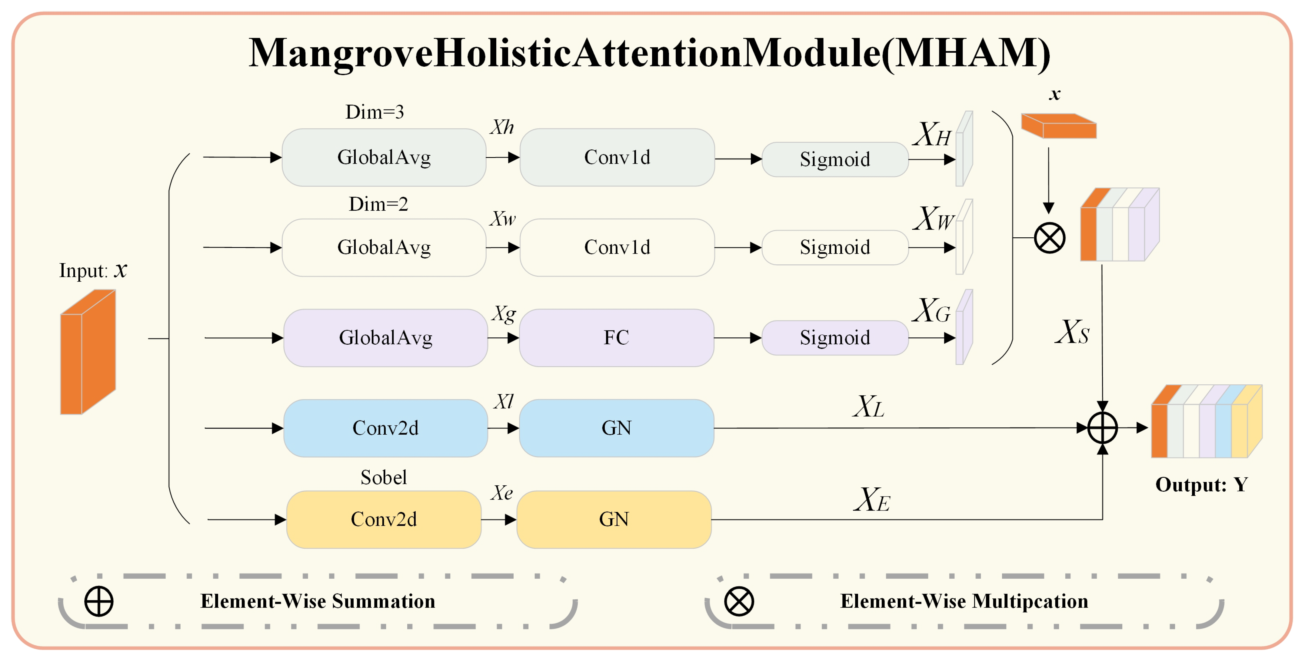
3.5. Mangrove Holistic Attention Module (MHAM)

Here, we provide a detailed explanation of the MHAM within the MHAGM, as shown in Figure 5. The structure of MHAM is illustrated in Figure 7. It consists of attention processing layers for the height and width dimensions, local feature extraction convolution layers, edge feature extraction convolution layers, and global feature extraction layers.

The attention processing layers extract features along the height and width dimensions, capturing long-range dependencies. This helps distinguish the overall morphology of different mangrove species.

The local feature extraction convolution layer focuses on fine-texture details of leaves and branches. It enhances the ability to differentiate subtle texture variations among similar species, improving fine-detail recognition.

The edge feature extraction convolution layer enhances contour detection. It aids in recognizing species with blurry edges or complex shapes, thus improving classification accuracy.

The global feature extraction layer captures overall image information, which aids in distinguishing the general structure of each species and enhances recognition in complex backgrounds.

(1) Height dimension attention

For the input feature map x, independent attention computation is performed along the height dimension. This is performed by applying a 1D convolution operation along the height, followed by normalization and a Sigmoid activation function. These steps generate the corresponding attention map $x_h$ for that dimension.The formula is as follows:

$$x_h=\mathrm{GlobalAvg}(x,\dim =3)$$

(12)

$$x_{\mathrm{H}}=\sigma \left(\mathrm{GN}\left(\mathrm{Conv}1\mathrm{D}\left(x_h\right)\right)\right)$$

(13)

where Dim = 3 indicates that the mean is computed along the width dimension. $Conv1\mathrm{D}(·)$ refers to the convolution operation applied along the channel dimension, which is used to calculate the attention along the height. $GN(·)$ stands for group normalization, which is applied to the feature map after the convolution. $\sigma$ represents the Sigmoid activation function, which outputs attention weights in the range [0, 1].

(2) Width dimension attention

Next, the mean along the height dimension of the image is calculated, and then a convolution operation is applied to compute the attention map along the width dimension. The formula is expressed as:

$$x_w=\mathrm{GlobalAvg}\left(x\right)$$

(14)

$$x_{\mathrm{W}}=\sigma \left(\mathrm{GN}\left(\mathrm{Conv}1\mathrm{D}\left(x_w\right)\right)\right)$$

(15)

where Dim = 2 indicates that the mean is computed along the height dimension. $Conv1\mathrm{D}(·)$ refers to the convolution operation applied along the channel dimension, which is used to calculate the attention along the width. $GN(·)$ represents group normalization, applied to the feature map after the convolution. $\sigma$ is the Sigmoid activation function, which outputs attention weights in the range [0, 1].

(3) Local texture feature extraction

Local features are extracted using a local convolution operation. A 3 × 3 convolution kernel is applied to the input feature map, extracting features from each local region. The computation process is as follows:

$$x_l=\mathrm{Conv}2\mathrm{D}\left(x\right)$$

(16)

$$x_{\mathrm{L}}=\sigma \left(\mathrm{FC}\left(\mathrm{ReLU}\left(\mathrm{FC}\left(x_l\right)\right)\right)\right)$$

(17)

where $\mathrm{Conv}2\mathrm{D}(·)$ refers to the 3 × 3 convolution operation, and $GN(·)$ stands for group normalization. $x_l$ represents the initially extracted local texture features, and $x_L$ denotes the final extracted local texture features.

(4) Edge feature extraction

Edge features are crucial for recognizing the morphology of mangrove species, particularly when species exhibit similar shapes or contours. To capture these edge details, this paper uses the Sobel edge detection kernel, which highlights high-gradient areas such as sharp leaf edges. These edges are then processed with group normalization for further feature extraction.

While modern deep learning methods can learn edge features automatically, Sobel edge detection remains valuable in this setting due to its simplicity and efficiency. It explicitly extracts sharp, well-defined edges, which are crucial for accurately identifying mangrove species.

The MHAM module, with its multi-level attention mechanism, also focuses on edge-like features during training. This raises the question of whether Sobel becomes redundant when combined with MHAM. In fact, Sobel and MHAM complement each other rather than overlap. Sobel provides explicit, predefined edge features, which serve as a solid foundation for further refinement. Meanwhile, MHAM enhances these features by applying both local and global attention to emphasize important boundaries. This combination allows the model to better capture fine-scale details and resolve challenging species boundaries, especially in complex cases where species overlap.

After extracting the edge information, group normalization is applied to obtain the edge features. The computation process is as follows:

$$x_e={\mathrm{Conv}2\mathrm{D}}_{\mathrm{sobel}}\left(x\right)$$

(18)

$$x_{\mathrm{E}}=\mathrm{GN}\left(x_e\right)$$

(19)

where $Conv2D_{sobel}(·)$ refers to the convolution operation using the Sobel kernel, and $GN(·)$ is group normalization, which is applied to process the convolution results.

(5) Global feature extraction

Global features are essential for identifying the large-scale patterns and spatial layouts of mangrove species. For instance, features such as crown size and tree height play a crucial role in distinguishing different species. Global features are extracted using adaptive pooling, which compresses the spatial dimensions to obtain a global feature vector. This vector is then passed through two fully connected layers to obtain the global attention $x_G$. The formula is as follows:

$$x_g=\mathrm{GlobalPool}\left(x\right)$$

(20)

$$x_{\mathrm{G}}=\sigma \left(\mathrm{FC}\left(x_g\right)\right)$$

(21)

where $GlobalPool(·)$ refers to average pooling, $FC(·)$ represents the two fully connected layers, and $\sigma$ is the Sigmoid activation function, which outputs the global attention weights.

(6) Feature fusion

After computing the attention for height, width, and global dimensions, the three attention components are combined through element-wise multiplication to obtain the final spatial and channel attention. This refined attention map is subsequently applied to the original input feature map x to generate the final feature map $x_s$. The computation process is as follows:

$$x_{\mathrm{s}}=x\times x_{\mathrm{H}}\times x_{\mathrm{W}}\times x_{\mathrm{G}}$$

(22)

Finally, the local features and edge features are integrated with the attention-enhanced feature map through element-wise addition to obtain the final fused features. The computation process is as follows:

$$\mathrm{Y}=x_{\mathrm{s}}+x_{\mathrm{L}}+x_{\mathrm{E}}$$

(23)

4. Experimental Analysis

4.1. Dataset Construction

RGB Image Collection Using Drone Remote Sensing

In this paper, a DJI Mavic 3E drone equipped with a high-resolution RGB camera sensor was used to collect data on mangrove species in the Shankou Mangrove National Nature Reserve, located in Beihai, Guangxi, China. The data collection spanned from September 2023 to June 2024, with monthly flights conducted to capture seasonal variations in the mangrove ecosystem. The drone flew at a height of 10 m with a forward speed of 3 m per second. The dataset primarily focuses on mangrove species in the Shankou Mangrove National Nature Reserve, which exhibits typical subtropical mangrove ecosystem characteristics. These areas face similar environmental challenges and human disturbances as other mangrove regions globally, making the dataset highly relevant for broader ecological applications. However, it is important to note that the data were derived from a single region, and potential domain adaptation for other mangrove species or regions with different environmental conditions should be considered for global scalability.

To ensure comprehensive coverage, the dataset includes images of mangroves at various growth stages and across different seasons. It also captures instances of flooding and mud coverage following tidal changes, as well as the impacts of typhoons and shadow effects. These conditions reflect the ecological diversity of mangrove ecosystems and provide a robust foundation for training models that can handle variations in the appearance of mangrove species under diverse environmental factors.

Figure 8 presents several typical images of mangrove species collected in the Shankou Mangrove National Nature Reserve. Panels (a) to (e) depict Sonneratia apetala, Avicennia marina, Bruguiera gymnorhiza, Rhizophora stylosa, and Kandelia obovata, respectively.

As shown in

Table 1. Data information of MSIDBG.

Database Name	MSIDBG
Corresponding Author	Shaolin Guo
Data Authors	Xin Wang, Jia Lu, Shaolin Guo, Wenlong Dai
Data Time Range	2023–2024
Geographic Area	109°37′ E–109°47′ E, 21°28′22″ N–21°37′ N
Data Volume	1 TB
Data Format	*.JPEG

, it is a brief introduction to the basic information of the MSIDBG (Mangrove Species Identification Database for UAV Images).

4.2. Images Preprocessing

For data annotation, this study used the manual labeling tool LabelMe [30], under the guidance of mangrove experts. The crowns and leaves of different species in each image were meticulously labeled to ensure accuracy and precision in the annotations. Figure 9 shows an example of the annotated images.where Figure 9a is the original image and Figure 9b is the annotated image.

In this paper, to prepare the dataset for deep learning model training, a systematic approach was adopted to ensure model robustness and generalization. Initially, the images were preprocessed, including normalization, denoising, and augmentation techniques such as random rotations, cropping, and scaling to enrich the dataset and account for various environmental conditions. For model input, each selected image region was cropped to a size of 512 × 512 pixels, which aligns with the required dimension for the deep learning model. To ensure comprehensive training, we used a sliding window approach to extract a total of 2640 image patches from the original dataset.

The dataset was then split into training, validation, and testing sets. Specifically, 60% of the images (1584 patches) were allocated for training, 20% (528 patches) for validation, and the remaining 20% (528 patches) for testing. This division ensures a balanced distribution of images for both model training and evaluation, allowing the model to generalize effectively while minimizing overfitting. The validation set was used to fine-tune hyperparameters and monitor model performance during training, while the testing set provided an unbiased evaluation of the final model’s accuracy and robustness.

4.3. Network Training

The experiments were conducted on an Ubuntu 18.04.1 operating system, equipped with an NVIDIA GeForce RTX 3090 GPU(manufactured by NVIDIA Corporation) (with 24 GB of memory), using Python 3.8 and PyTorch 1.12 (supporting CUDA 11.3) as the experimental environment. During the model training phase, the batch size was set to 2, and Stochastic Gradient Descent (SGD) was chosen as the optimization algorithm. The momentum value was set to 0.9, and the weight decay coefficient was set to 0.0001 to ensure a stable learning process. The model underwent a total of 200 training epochs on the training set. To facilitate more effective model convergence, a dynamic learning rate adjustment strategy (the polynomial strategy) was employed, which allowed the learning rate to be automatically adjusted based on training progress, thereby accelerating the model’s convergence speed.

To evaluate the recognition performance of the proposed network, we use several model metrics: IoU, accuracy (Acc), mean accuracy (mAcc), overall accuracy (aAcc), and Mean Intersection over Union (mIoU).

Pixel accuracy (Acc) measures the proportion of correctly predicted pixels in the image segmentation task. It is defined as the ratio of correctly predicted pixels to the total number of pixels:

$$\mathrm{Acc}={\displaystyle \frac{{\sum }_{i=1}^{N}T{P}_i}{{\sum }_{i=1}^N{P}_i}}$$

(24)

where $T{P}_i$ is the number of true positive pixels for class $\mathit{i}$ and $P_i$ is the total number of pixels in class $\mathit{i}$.

Mean accuracy (mAcc) evaluates the average classification accuracy for each category in the image segmentation task. It reflects the model’s ability to correctly classify pixels for each category, averaged across all categories:

$$\mathrm{mAcc}={\displaystyle \frac{1}{C}}\sum _{i=1}^C{\displaystyle \frac{T{P}_i}{T{P}_i+F{N}_i}}$$

(25)

where $\mathit{C}$ is the number of classes, $T{P}_i$ is the number of true positive pixels for class $\mathit{i}$ and $F{N}_i$ is the false negative pixels for class $\mathit{i}$.

Overall accuracy (aAcc) measures the overall classification accuracy of all pixels in the image, without distinguishing between categories. It is computed as the ratio of the total number of correctly predicted pixels to the total number of pixels in the image:

$$\mathrm{aAcc}={\displaystyle \frac{{\sum }_{i=1}^{N}T{P}_i}{{\sum }_{i=1}^N{T}_i}}$$

(26)

where $T_i$ is the total number of pixels in the image, and $T{P}_i$ is the number of true positive pixels.

Mean Intersection over Union (mIoU) is a widely used metric in image segmentation tasks. It measures the quality of the model’s predictions for each category and takes the average across all categories. It is defined as the average of the IoU for each class:

$$\mathrm{mIoU}={\displaystyle \frac{1}{C}}\sum _{i=1}^C{\displaystyle \frac{T{P}_i}{T{P}_i+F{P}_i+F{N}_i}}$$

(27)

where $T{P}_i$ is the number of true positive pixels for class $\mathit{i}$, $F{P}_i$ is the number of false positive pixels, and $F{N}_i$ is the number of false negative pixels for class $\mathit{i}$.

4.4. Experimental Results

4.4.1. Ablation Experiments

We perform an ablation study on mangrove species database MSIDBG. The experimental results are shown in

Table 2. Results of ablation experiments (Acc).

Methods	Acc (%) per Category					mAcc (%)	aAcc (%)
	K. obovata	S. apetala	A. marina	B. gymnorhiza	R. stylosa
Baseline	93.48	73.74	60.99	96.2	97.47	84.38	92.58
Baseline + MHAM	93.31	93.88	74.57	96.09	97.12	91	94.51
Baseline + MHGSEM	94.00	95.81	80.85	96.02	97.55	92.85	84.97
Baseline + MHAM + MHGSEM + MHAGM	94.76	96.83	82.96	96.81	97.99	93.87	95.89

, show pixel accuracy (Acc) performance under different module combinations. We use DeepLab v3 as the baseline model.

In our experiments conducted on the MSIDBG dataset, we evaluate the performance of the model using two key metrics: Intersection over Union (IoU) and accuracy (Acc). These metrics are calculated for five distinct mangrove species: Sonneratia apetala, Avicennia marina, Bruguiera gymnorhiza, Rhizophora stylosa, and Kandelia obovata. The background class is excluded from IoU and Acc calculations. This exclusion aligns with the dataset’s design, which focuses on mangrove species segmentation rather than background differentiation. Our primary goal is to assess the model’s ability to distinguish among different mangrove species in complex ecological environments.

From Table 2, we see that the inclusion of various modules significantly improves the recognition accuracies of the MHAGFNet. The baseline model performs poorly on the Avicennia marina category, with an accuracy of only 60.99%. After incorporating the MHAM, the accuracy for this category increases to 74.57%, and the model’s mean accuracy (mAcc) improves from 84.38% to 91%, demonstrating that MHAM effectively enhances the model’s ability to extract detailed features across different categories. With the further addition of the MHGSEM, the accuracy for Avicennia marina continues to rise to 80.85%, leading to a significant overall improvement in classification performance, with the average accuracy (mAcc) reaching 92.85%. This suggests that the MHGSEM plays a crucial role in capturing fine-grained features and enhancing local information. When all modules (MHAM, MHGSEM, and MHAGM) are combined, the proposed MHAGFNet achieves optimal performance, and recognition accuracies of all categories are further improved, especially for Avicennia marina, where the recognition accuracy reaches 82.96%. In addition, the mean accuracy (mAcc) and overall accuracy (aAcc) reach 93.87% and 95.89%, respectively. This indicates that the combination of modules can further improve the MHAGFNet’s recognition capability for various mangroves species in complex scenarios.

Table 3. Results of ablation experiments (IoU).

Methods	IoU (%) per Category					mIoU (%)
	K. obovata	S. apetala	A. marina	B. gymnorhiza	R. stylosa
Baseline	81.9	79.25	66.96	92.4	93.75	82.85
Baseline + MHAM	87.1	80.84	67.75	92.74	94.14	84.51
Baseline + MHGSEM	87.22	86.02	73.2	93.14	94.38	86.80
Baseline + MHAM + MHGSEM + MHAGM	89.6	85.94	76.11	95.33	95.25	88.45

presents the ablation experimental results on mangrove species recognition, showcasing the intersection over union (IoU) performance under different module combinations.

From Table 3, we see that the baseline model exhibits poor IoU performance for certain species, such as Sonneratia apetala and Avicennia marina, with values of 79.25% and 66.96%, respectively. After introducing the MHAM, the IoU for Sonneratia apetala and Avicennia marina improved to 80.84% and 67.75%, respectively, while the mIoU increased from the baseline value of 82.85% to 84.51%. This indicates that the MHAM improves the model’s segmentation capabilities in complex mangrove environments. When the MHGSEM is added, the IoU for Avicennia marina increases to 73.2%, and Sonneratia apetala’s IoU increases to 86.02%, achieving a mean IoU (mIoU) of 86.80%. These results demonstrate that the MHGSEM plays a positive role in multi-scale feature fusion and capturing local detailed information, thereby further enhancing segmentation accuracy. Ultimately, the combination of the MHAM, MHGSEM, and MHAGM resulted in optimal IoU performance, with Avicennia marina achieving an IoU of 76.11% and Kandelia obovata an IoU of 89.6%, resulting in a mIoU of 88.45%. This indicates that the integration of all modules significantly improves the MHAGFNet’s segmentation effectiveness for different mangrove species, particularly excelling in boundary segmentation and complex morphological features.

To more intuitively demonstrate the effectiveness of the modules proposed in this paper, we visualize the results of both individual modules and their combinations, as shown in Figure 10. The circles in the figure indicate the segmentation error for each image.

From Figure 10, the baseline model exhibits notable limitations in accurately segmenting mangrove species, particularly when distinguishing subtle morphological differences. This results in large misclassified regions and unclear boundaries between species, especially in overlapping or complex environments. These challenges are compounded by varying environmental factors such as light angles, shadows, and reflections.

When the MHAM module is introduced, the model significantly improves in recognizing mangrove species, particularly small target species. MHAM enhances both local and global feature extraction through its multi-level attention mechanism, which combines spatial, channel, and edge features. As illustrated in Figure 10a,b, in the case of Sonneratia apetala, a species with relatively subtle leaf shape differences compared to Avicennia marina, MHAM helps improve recognition by capturing fine-scale details with its edge detection convolution and local texture features. This results in improved accuracy for small target recognition. However, it is important to note that MHAM does not uniformly improve performance across all species. In some cases, such as Rhizophora stylosa (as illustrated in Figure 10e), the model’s performance in boundary delineation remains suboptimal, likely due to the overlap of leaf characteristics with Sonneratia apetala, especially under varying light conditions. This example suggests that while MHAM enhances small target detection, its effectiveness may vary across different mangrove species.

Incorporating the MHGSEM module further enhances the model’s ability to handle multi-scale features, particularly in distinguishing mangrove species with subtle morphological differences. As illustrated in Figure 10c, Kandelia obovata, which shares leaf morphology similarities with Sonneratia apetala under certain conditions, benefits from the MHGSEM module’s enhanced spatial and channel attention mechanisms. This module effectively captures both global and local features, improving the overall differentiation of species. However, similar to MHAM, MHGSEM also has its limitations. The Rhizophora stylosa species, despite its relatively distinct leaf morphology, still poses challenges for boundary detection, especially when there are variations in shadow or light intensity. This suggests that while MHGSEM improves the overall model performance, it still faces difficulties in environments with significant light variation.

Finally, by integrating all modules based on the MHAGM (which combines MHAM and MHGSEM), the model achieves a more robust solution. The fusion of global and local features improves the recognition accuracy of small targets and enhances the delineation of complex species boundaries. As illustrated in Figure 10c,d, in the case of Avicennia marina, the model demonstrates substantial improvement in accurately identifying the species’ boundaries and distinguishing it from other species, especially in environments where mangrove species overlap. However, despite these improvements, the model still encounters some failure cases. Specifically, the Sonneratia apetala and Avicennia marina species are occasionally misclassified due to their similar leaf shapes and colors, particularly in images with low resolution or under poor lighting conditions.

4.4.2. Comparison Experiments

In this section, we will conduct comparison experiments using both the public dataset and our self-created mangrove dataset, MSIDBG.

A. Comparison experiments on public dataset

To evaluate the performance roundly, we compare our method with some state-of-the-art methods on the Potsdam dataset [31] and Loveda-Rural dataset [32].

The compared experimental results (Acc) on the Potsdam dataset are presented in

Table 4. Compared experimental results (Acc) on Potsdam dataset.

Methods	Acc (%) per Category						mAcc (%)	aAcc (%)
	Impervious_Surface	Building	Low_Vegetation	Tree	Car	Clutter
FCN [21]	92.94	96.74	90.19	87.04	95.71	49.16	85.30	90.47
DeepLab v3 [22]	93.00	97.33	88.71	88.08	95.25	52.77	85.86	90.66
DeepLab v3+ [23]	92.30	97.24	89.68	86.02	95.32	52.95	85.59	90.27
UperNet [24]	92.73	97.06	89.72	87.91	95.59	54.76	86.30	90.78
Mobilenetv2 [25]	91.81	96.88	87.40	85.91	92.59	49.37	83.99	89.34
OCRNet [26]	92.29	97.38	89.28	85.11	94.13	47.76	84.32	89.82
DMNet [27]	93.15	97.06	89.15	87.94	95.89	56.93	86.68	90.89
Swin-T [28]	93.38	97.06	89.75	84.5	93.27	50.17	84.69	90.17
Ours	93.81	97.42	89.39	90.61	95.72	57.83	87.46	91.49

.

From Table 4, we see that the proposed MHAGFNet achieves a high mean accuracy (mAcc) of 87.46%, particularly excelling in the categories of buildings and trees compared to other models. Specifically, the MHAGFNet’s accuracy for the impervious surface category is 93.81%, and it reaches 97.42% for the building category, demonstrating exceptional capability in building recognition. Although the accuracy for the low vegetation and clutter categories is relatively lower at 89.39% and 57.83%, respectively, the MHAGFNet still achieves commendable performance in vehicle recognition. Overall, the proposed MHAGFNet exhibits strong generalization ability in handling complex scenes and small objects, particularly enhancing precision in the classification of buildings and trees, showcasing excellent detail handling and boundary delineation capabilities.

The compared experimental results (Acc) on the Loveda-Rural dataset are shown in

Table 5. Compared experimental results(Acc) on Loveda-Rural dataset.

Methods	Acc (%) per Category							mAcc (%)	aAcc (%)
	Background	Building	Road	Water	Barren	Forest	Agricultural
FCN [21]	87.11	62.82	25.77	77.22	13.37	30.23	52.72	49.89	67.42
DeepLab v3 [22]	92.94	64.09	26.93	72.91	16.24	11.23	52.05	48.06	68.44
DeepLab v3+ [23]	84.84	60.29	29.90	79.13	15.39	39.24	52.38	51.6	67.11
UperNet [24]	96.20	45.38	22.38	59.36	10.24	3.08	51.05	41.1	66.52
Mobilenetv2 [25]	87.04	64.95	36.23	86.57	17.40	39.50	49.10	54.4	68.34
OCRNet [26]	91.53	69.85	29.07	76.63	19.87	14.66	52.34	50.57	68.93
DMNet [27]	92.13	57.71	31.76	75.03	16.81	13.60	49.99	48.14	67.74
Swin-T [28]	87.04	64.95	36.23	86.57	17.4	39.5	49.1	54.40	68.34
Ours	93.84	64.66	37.27	75.50	20.98	41.37	50.02	54.81	70.53

.

From Table 5, we see that the proposed MHAGFNet achieves a mean accuracy (mAcc) of 54.81%, demonstrating significantly better performance than other models, especially in the categories of roads and buildings. Specifically, the accuracy for the background category is 93.84%, indicating strong recognition capabilities. The accuracy for the building category is 64.66%, which, while relatively lower compared to some models, still shows a competitive edge. The road category achieves an accuracy of 37.27%, marking an improvement over other methods, particularly under complex scenes, demonstrating some generalization ability. However, the accuracies for the water and barren categories are 75.5% and 20.98%, respectively, which fall short of certain comparative models. In contrast, the forest and agricultural categories show improved performance, with accuracies of 41.37% and 50.02%. Overall, although there is room for improvement in recognizing certain categories, the proposed MHAGFNet demonstrates strong potential in handling multiple categories, particularly excelling in road classification accuracy. These results indicate that the proposed MHAGFNet plays a crucial role in effectively classifying complex backgrounds and various land features.

The segmentation results (IoU) on the Potsdam dataset are presented in

Table 6. Compared experimental results (IoU) on the Potsdam dataset.

Methods	IoU (%) per Category						mIoU (%)
	Impervious_Surface	Building	Low_Vegetation	Tree	Car	Clutter
FCN [21]	87.05	93.32	76.04	79.32	92.19	40.5	78.07
DeepLab v3 [22]	87.36	93.14	76.54	79.63	91.9	42.56	78.52
DeepLab v3+ [23]	86.69	92.8	75.93	79.02	91.47	41.52	77.91
Upernet [24]	87.06	93.3	77.17	79.6	91.55	44.79	78.91
Mobilenetv2 [25]	85.31	91.29	75.15	77.2	88.08	37.48	75.75
OCRnet [26]	86.17	90.9	75.85	77.51	89.37	40.65	76.74
Dmnet [27]	87.49	93.22	77.21	79.45	92.18	46.48	79.34
Swin-T [28]	86.25	92.5	76.71	78.0	89.59	40.64	77.28
Ours	87.94	93.23	76.08	83.61	91.72	47.94	80.09

.

From Table 6, we see that the proposed MHAGFNet achieves a high mIoU of 80.09%, with a significant improvement in the tree category, where the IoU reaches 83.61%. Specifically, the IoU for the impervious surface category is 87.94%, slightly higher than other comparative models, while the IoU for the building category is 93.23%, which is among the best across all methods. Although the IoU for the low vegetation category is 76.08%, which is somewhat lower, the overall segmentation performance remains robust. In the car category, the IoU reaches 91.72%, demonstrating excellent classification performance, and the clutter category shows an IoU of 47.94%, performing well compared to other models. In summary, the proposed MHAGFNet demonstrates strong capabilities in handling complex scenes and capturing details, particularly excelling in the segmentation of tree and clutter categories, indicating that the introduced modules play a vital role in enhancing IoU performance.

The segmentation results (IoU) on the Loveda-Rural dataset are shown in

Table 7. Compared experimental results (IoU) on the Loveda-Rural dataset.

Methods	IoU (%) per Category							mIoU (%)
	Background	Building	Road	Water	Barren	Forest	Agricultural
FCN [21]	55.84	53.36	24.66	61.01	11.92	23.06	48.43	39.75
DeepLab v3 [22]	57.78	54.26	25.87	63.47	14.84	10.48	48.87	39.31
DeepLab v3+ [23]	54.67	50.92	28.73	63.69	13.94	25.87	48.21	40.86
Upernet [24]	56.5	42.18	21.66	54.95	9.88	3.02	48.17	33.76
Mobilenetv2 [25]	57.34	44.65	34.38	66.26	14.84	28.09	46.94	41.79
OCRnet [26]	58.18	56.48	27.46	64.23	16.93	13.28	49.03	40.8
Dmnet [27]	57.24	45.7	30.41	63.2	14.86	12.09	47.25	38.62
Swin-T [28]	57.34	44.65	34.38	66.26	14.84	28.09	46.94	41.79
Ours	59.68	44.39	34.95	67.55	17.71	28.84	48.47	43.08

.

From Table 7, we see that the proposed MHAGFNet achieves a mIoU of 43.08% for the segmentation task. Specifically, the IoU for the background category is 59.68%, outperforming most comparative models and demonstrating strong background segmentation capability. The IoU for the building category is 44.39%, which is relatively lower compared to other models but still competitive. The road category shows an IoU of 34.95%, indicating a noticeable improvement compared to other methods, particularly in classification accuracy within complex scenes. The water category excels with an IoU of 67.55%, ranking high among all methods. However, the barren category has a lower IoU of 17.71%, suggesting that segmentation for this category requires further optimization. The forest and agricultural categories achieve IoUs of 28.84% and 48.47%, respectively, reflecting the model’s ability to segment various land cover features. Overall, while there is room for improvement in certain categories, the proposed MHAGFNet demonstrates promising potential in segmentation tasks involving complex backgrounds and multiple features, particularly excelling in background and water segmentation, indicating the important role of the introduced modules in enhancing segmentation accuracy.

B. Comparison experiments on mangrove dataset (MSIDBG)

In order to evaluate the superiority of the proposed MHAGFNet, we compare our method with some state-of-the-art methods on the mangrove dataset (MSIDBG). The recognition accuracy (Acc) results on the mangrove dataset are presented in

Table 8. Compared experimental results (Acc) on the MSIDBG dataset.

Methods	Acc (%) per Category					mAcc (%)	aAcc (%)
	K. obovata	S. apetala	A. marina	B. gymnorhiza	R. stylosa
FCN [21]	93.15	96.79	73.22	96.27	97.46	91.38	94.86
DeepLab v3 [22]	86.38	92.71	71.49	96.53	97.03	82.55	93.80
DeepLab v3+ [23]	93.48	73.74	60.99	96.2	97.47	84.38	92.58
Upernet [24]	93.4	70.09	56.96	96.23	96.01	82.54	92.72
Mobilenetv2 [25]	91.94	91.12	66.55	95.56	97.15	88.46	93.79
OCRnet [26]	91.63	96.78	81.16	95.93	97.39	92.58	94.51
DMnet [27]	93.89	87.13	56.4	96.36	97.84	84.32	94.50
Swin-T [28]	96.82	93.47	65.62	96.08	97.23	89.84	94.44
Ours	94.76	96.83	82.96	96.81	97.99	93.87	95.89

.

From Table 8, we see that the proposed MHAGFNet demonstrates excellent performance across all categories. Notably, the MHAGFNet achieves a significantly higher accuracy of 82.96% for the Avicennia marina category compared to other methods, such as FCN (73.22%) and DeepLab v3+ (60.99%). This improvement can be attributed to the superior ability of MHAGFNet to capture the detailed features of this species. Overall, MHAGFNet’s mean accuracy (mAcc) reaches 93.87%, surpassing most comparative models, including FCN (91.38%) and DeepLab v3 (82.55%). Additionally, the overall accuracy (aAcc) achieves 95.89%, indicating that MHAGFNet provides more stable segmentation performance across the entire dataset.

For a clearer presentation of our experimental results on the MSIDBG dataset, the corresponding confusion matrix is illustrated in Figure 11. The confusion matrix represents the segmentation performance of our model for five mangrove species, where the color intensity indicates the accuracy of classification: darker colors represent higher accuracy, while lighter colors represent lower accuracy.

The compared experimental results (IoU) on the mangrove dataset are shown in

Table 9. Compared experimental results (IoU) on the MSIDBG dataset.

Methods	IoU (%)					mIoU (%)	Parameters (M)	Flops (G)
	K. obovata	S. apetala	A. marina	B. gymnorhiza	R. stylosa
FCN [21]	87.05	84.37	70.14	93.1	94.45	85.62	47.134	15.83
DeepLab v3 [22]	81.9	79.25	66.96	92.4	93.75	82.85	65.749	21.59
DeepLab v3+ [23]	86.89	66.2	60.94	92.98	90.47	79.49	41.22	14.13
Upernet [24]	86.47	62.25	55.16	91.87	91.31	77.41	64.052	18.97
Mobilenetv2 [25]	84.42	76.89	60.07	91.81	93.27	81.29	15.085	5.5
OCRnet [26]	85.69	84.87	66.96	92.43	93.84	84.75	30.71	49.05
DMnet [27]	87.64	81.9	55.21	93.43	94.75	82.42	50.87	15.7
Swin-T [28]	84.11	83.93	63.16	92.01	94.1	83.46	59.018	59.88
Ours	89.6	85.94	76.11	95.33	95.25	88.45	51.401	21.36

.

Table 9 further demonstrates the superiority of the proposed MHAGFNet, which achieves high IoU scores across all categories, particularly in the Avicennia marina (76.11%) and Kandelia obovata (89.6%) categories, where its performance significantly outperforms other models, such as DeepLab v3 (66.96%) and FCN (70.14%). This indicates that the proposed MHAGFNet not only excels in species recognition but also shows improved boundary segmentation. Moreover, the MHAGFNet’s mIoU values reach 88.45%, representing a significant improvement over other established methods, such as DeepLab v3 (74.25%) and Upernet (69.3%). The high IoU values indicate that the proposed MHAGFNet effectively distinguishes subtle differences between categories at the pixel level, which is particularly crucial in the complex mangrove environment.

In addition to the segmentation performance, we also evaluate the computational efficiency of each method, as indicated by the number of parameters (in millions) and FLOPs (floating-point operations in gigaflops). Our method achieves a reasonable balance between accuracy and efficiency with 51.401 million parameters and 21.36 GFLOPs, which is competitive compared to other methods.

To more intuitively observe the differences between the proposed MHAGFNet and other methods, we present a data visualization comparing our method with several representative techniques.

As shown in Figure 12, Figure 12a,b clearly show that other methods significantly lack accuracy in classifying mangroves in complex environments, particularly performing poorly when classifying small target mangrove species. As illustrated in Figure 12d,e, other methods fail to accurately identify small-target Rhizophora stylosa in overlapping regions, whereas our approach achieves more precise recognition. In the comparison between Figure 12b–d, we observe that due to the morphological similarities between mangrove species, other methods frequently encounter issues of misclassification and vague segmentation boundaries, and in some cases, even produce trapezoidal boundaries, which severely compromise the model’s recognition performance. In contrast, the proposed MHAGFNet not only demonstrates clearer and more defined segmentation boundaries but also significantly improves classification accuracy, effectively addressing challenges in complex environments. Through these comparisons, the proposed MHAGFNet showcases its superiority in mangrove species recognition, capturing subtle features and precisely delineating the boundaries of different species.

5. Conclusions

In this paper, we propose a novel approach, MHAGFNet, designed to enhance mangrove species recognition in complex ecological environments. MHAGFNet integrates several innovative modules that significantly improve its adaptability and accuracy in species classification. The Multi-Scale Feature Fusion Module (MSFFM) plays a crucial role in enhancing the network’s ability to capture subtle differences in leaf shape and canopy structure, making it particularly suited for precise classification tasks. The Multi-Head Attention Guide Module (MHAGM), which combines the Multi-Head Attention Module (MHAM) with the Multi-Head Global Semantic Enhancement Module (MHGSEM), further enriches the extraction of local, edge, and global features, improving the model’s capacity to recognize both global structures and detailed features, especially in complex and dynamic environments.

However, despite the promising results, there are limitations to the proposed method. The performance of MHAGFNet may be compromised under extreme environmental conditions, such as intense midday sunlight causing high water reflection, or when significant wind movement affects canopy stability. Additionally, the model may struggle with challenging scenarios, such as unusual lighting angles or completely submerged roots. In these situations, the network’s stability and sensitivity could be impacted, leading to potential misclassification.

To address these limitations, future work could focus on enhancing the model’s robustness to variations in lighting conditions and complex environmental factors. One potential direction is to explore advanced techniques, such as image super-resolution (SR), which can improve the quality of low-resolution images and enable the model to capture the fine details and features essential for accurate species classification. Additionally, incorporating temporal data or sensor fusion methods could further strengthen the model’s ability to adapt to dynamic environmental conditions, such as lighting variations, water reflections, and canopy movement. Further development of adaptive mechanisms to handle challenging scenarios, such as submerged structures or species with similar visual characteristics, would be beneficial for improving model stability and accuracy under extreme conditions.

References

1. Trialfhianty, T.I.; Muharram, F.W.; Quinn, C.H.; Beger, M. Spatial multi-criteria analysis to capture socio-economic factors in mangrove conservation. Mar. Policy 2022, 141, 105094. [Google Scholar] [CrossRef]
2. Su, J.; Friess, D.; Gasparatos, A. A meta-analysis of the ecological and economic outcomes of mangrove restoration. Nat. Commun. 2021, 12, 5050. [Google Scholar] [CrossRef] [PubMed]
3. Jakovac, C.C.; Latawiec, A.E.; Lacerda, E.; Lucas, I.L.; Korys, K.A.; Iribarrem, A.; Malaguti, G.A.; Turner, R.K.; Luisetti, T.; Strassburg, B.B.N. Costs and carbon benefits of mangrove conservation and restoration: A global analysis. Ecol. Econ. 2020, 176, 106758. [Google Scholar] [CrossRef]
4. Zeng, Y.; Friess, D.A.; Sarira, T.V.; Siman, K.; Koh, L.P. Global potential and limits of mangrove blue carbon for climate change mitigation. Curr. Biol. 2021, 31, 1737–1743. [Google Scholar] [CrossRef] [PubMed]
5. Song, S.; Ding, Y.; Li, W.; Meng, Y.; Zhou, J.; Gou, R.; Zhang, C.; Ye, S.; Saintilan, N.; Krauss, K.W.; et al. Mangrove reforestation provides greater blue carbon benefit than afforestation for mitigating global climate change. Nat. Commun. 2023, 14, 756. [Google Scholar] [CrossRef]
6. Marlianingrum, P.R.; Kusumastanto, T.; Adrianto, L.; Fahrudin, A. Valuing habitat quality for managing mangrove ecosystem services in coastal Tangerang District, Indonesia. Mar. Policy 2021, 133, 104747. [Google Scholar] [CrossRef]
7. Aburto-Oropeza, O.; Ezcurra, E.; Danemann, G.; Valdez, V.; Murray, J.; Sala, E. Mangroves in the Gulf of California increase fishery yields. Proc. Natl. Acad. Sci. USA 2008, 105, 10456–10459. [Google Scholar] [CrossRef]
8. Boonman, C.C.; Serra-Diaz, J.M.; Hoeks, S.; Guo, W.Y.; Enquist, B.J.; Maitner, B.; Malhi, Y.; Merow, C.; Buitenwerf, R.; Svenning, J.C. More than 17,000 tree species are at risk from rapid global change. Nat. Commun. 2024, 15, 166. [Google Scholar] [CrossRef]
9. Maurya, K.; Mahajan, S.; Chaube, N. Remote sensing techniques: Mapping and monitoring of mangrove ecosystem—A review. Complex Intell. Syst. 2021, 7, 2797–2818. [Google Scholar] [CrossRef]
10. Tomlinson, P.B. The Botany of Mangroves; Cambridge University Press: Cambridge, UK, 2016. [Google Scholar]
11. Fu, B.; He, X.; Yao, H.; Liang, Y.; Deng, T.; He, H.; Fan, D.; Lan, G.; He, W. Comparison of RFE-DL and stacking ensemble learning algorithms for classifying mangrove species on UAV multispectral images. Int. J. Appl. Earth Obs. Geoinf. 2022, 112, 102890. [Google Scholar] [CrossRef]
12. Manna, S.; Raychaudhuri, B. Mapping distribution of Sundarban mangroves using Sentinel-2 data and new spectral metric for detecting their health condition. Geocarto Int. 2020, 35, 434–452. [Google Scholar] [CrossRef]
13. Setyadi, G.; Pribadi, R.; Wijayanti, D.P.; Sugianto, D.N. Mangrove diversity and community structure of Mimika District, Papua, Indonesia. Biodivers. J. Biol. Divers. 2021, 22. [Google Scholar] [CrossRef]
14. Cao, J.; Leng, W.; Liu, K.; Liu, L.; He, Z.; Zhu, Y. Object-based mangrove species classification using unmanned aerial vehicle hyperspectral images and digital surface models. Remote Sens. 2018, 10, 89. [Google Scholar] [CrossRef]
15. Zulfa, A.; Norizah, K.; Hamdan, O.; Faridah-Hanum, I.; Rhyma, P.; Fitrianto, A. Spectral signature analysis to determine mangrove species delineation structured by anthropogenic effects. Ecol. Indic. 2021, 130, 108148. [Google Scholar] [CrossRef]
16. Wang, X.; Tan, L.; Fan, J. Performance evaluation of mangrove species classification based on multi-source Remote Sensing data using extremely randomized trees in Fucheng Town, Leizhou city, Guangdong Province. Remote Sens. 2023, 15, 1386. [Google Scholar] [CrossRef]
17. Cao, J.; Liu, K.; Zhuo, L.; Liu, L.; Zhu, Y.; Peng, L. Combining UAV-based hyperspectral and LiDAR data for mangrove species classification using the rotation forest algorithm. Int. J. Appl. Earth Obs. Geoinf. 2021, 102, 102414. [Google Scholar] [CrossRef]
18. Zhen, J.; Mao, D.; Shen, Z.; Zhao, D.; Xu, Y.; Wang, J.; Jia, M.; Wang, Z.; Ren, C. Performance of XGBoost Ensemble Learning Algorithm for Mangrove Species Classification with Multisource Spaceborne Remote Sensing Data. J. Remote Sens. 2024, 4, 0146. [Google Scholar] [CrossRef]
19. Yang, Y.; Meng, Z.; Zu, J.; Cai, W.; Wang, J.; Su, H.; Yang, J. Fine-scale mangrove species classification based on uav multispectral and hyperspectral remote sensing using machine learning. Remote Sens. 2024, 16, 3093. [Google Scholar] [CrossRef]
20. Cheng, Y.; Yan, J.; Zhang, F.; Li, M.; Zhou, N.; Shi, C.; Jin, B.; Zhang, W. Surrogate modeling of pantograph-catenary system interactions. Mech. Syst. Signal Process. 2025, 224, 112134. [Google Scholar] [CrossRef]
21. Lu, Y.; Chen, Y.; Zhao, D.; Chen, J. Graph-FCN for image semantic segmentation. In Advances in Neural Networks, Proceedings of the International Symposium on Neural Networks, Moscow, Russia, 10–12 July 2019; Springer: Berlin/Heidelberg, Germany, 2019; pp. 97–105. [Google Scholar]
22. Chen, L.C.; Papandreou, G.; Kokkinos, I.; Murphy, K.; Yuille, A.L. Deeplab: Semantic image segmentation with deep convolutional nets, atrous convolution, and fully connected crfs. IEEE Trans. Pattern Anal. Mach. Intell. 2017, 40, 834–848. [Google Scholar] [CrossRef]
23. Liu, Y.; Bai, X.; Wang, J.; Li, G.; Li, J.; Lv, Z. Image semantic segmentation approach based on DeepLabV3 plus network with an attention mechanism. Eng. Appl. Artif. Intell. 2024, 127, 107260. [Google Scholar] [CrossRef]
24. Xiao, T.; Liu, Y.; Zhou, B.; Jiang, Y.; Sun, J. Unified perceptual parsing for scene understanding. In Proceedings of the European Conference on Computer Vision (ECCV), Munich, Germany, 8–14 September 2018; pp. 418–434. [Google Scholar]
25. Howard, A.G. Mobilenets: Efficient convolutional neural networks for mobile vision applications. arXiv 2017, arXiv:1704.04861. [Google Scholar]
26. Yuan, Y.; Chen, X.; Chen, X.; Wang, J. Segmentation Transformer: Object-Contextual Representations for Semantic Segmentation. arXiv 1909, arXiv:1909.11065. [Google Scholar]
27. He, J.; Deng, Z.; Qiao, Y. Dynamic multi-scale filters for semantic segmentation. In Proceedings of the IEEE/CVF International Conference on Computer Vision, Seoul, Republic of Korea, 27 October–2 November 2019; pp. 3562–3572. [Google Scholar]
28. Liu, Z.; Lin, Y.; Cao, Y.; Hu, H.; Wei, Y.; Zhang, Z.; Lin, S.; Guo, B. Swin transformer: Hierarchical vision transformer using shifted windows. In Proceedings of the IEEE/CVF International Conference on Computer Vision, Montreal, BC, Canada, 11–17 October 2021; pp. 10012–10022. [Google Scholar]
29. He, K.; Zhang, X.; Ren, S.; Sun, J. Deep residual learning for image recognition. In Proceedings of the IEEE Conference on Computer Vision and Pattern Recognition, Las Vegas, NV, USA, 27–30 June 2016; pp. 770–778. [Google Scholar]
30. Russell, B.C.; Torralba, A.; Murphy, K.P.; Freeman, W.T. LabelMe: A database and web-based tool for image annotation. Int. J. Comput. Vis. 2008, 77, 157–173. [Google Scholar] [CrossRef]
31. Rottensteiner, F.; Sohn, G.; Gerke, M.; Wegner, J.D. ISPRS semantic labeling contest. ISPRS LeopoldshÖhe Germany 2014, 1, 4. [Google Scholar]
32. Wang, J.; Zheng, Z.; Ma, A.; Lu, X.; Zhong, Y. LoveDA: A remote sensing land-cover dataset for domain adaptive semantic segmentation. arXiv 2021, arXiv:2110.08733. [Google Scholar]
Figure 1. Mangrove growth environment.
Symmetry 17 00461 g001
Figure 2. Examples of several typical mangrove species.
Symmetry 17 00461 g002
Figure 3. The architecture of proposed MHAGFNet.
Symmetry 17 00461 g003
Figure 4. Multi-Scale Feature Fusion Module.
Symmetry 17 00461 g004
Figure 5. Multi-Head Attention Guide Module.
Symmetry 17 00461 g005
Figure 6. Multi-Head Global Spatial Enhancement Module.
Symmetry 17 00461 g006
Figure 7. Mangrove holistic attention module.
Symmetry 17 00461 g007
Figure 8. Typical examples of mangrove species collected.
Symmetry 17 00461 g008
Figure 9. Example of labeled mangrove species images.
Symmetry 17 00461 g009
Figure 10. Visual comparison of ablation experiments.
Symmetry 17 00461 g010
Figure 11. Visual of the confusion matrix.
Symmetry 17 00461 g011
Figure 12. Visual comparison of comparison experiments.
Symmetry 17 00461 g012