Article

Functional Time Series Analysis Using Single-Index L1-Modal Regression

1
Department of Mathematics, College of Science, King Khalid University, Abha 62529, Saudi Arabia
2
Department of Mathematical Sciences, College of Science, Princess Nourah Bint Abdulrahman University, P.O. Box 84428, Riyadh 11671, Saudi Arabia
*
Author to whom correspondence should be addressed.
Symmetry 2025, 17(3), 460; https://doi.org/10.3390/sym17030460
Submission received: 17 February 2025 / Revised: 12 March 2025 / Accepted: 14 March 2025 / Published: 19 March 2025
(This article belongs to the Section Mathematics)

Abstract

:
A new predictor in functional time series (FTS ) is considered. It is based on the asymmetric weighting function of quantile regression. More precisely, we assume that FTS is generated from a single-index model that permits the observation of endogenous–exogenous variables by combining the nonparametric model with a linear one. In parallel, the L 1 -modal predictor is estimated using the M-estimation of the derivative of the conditional quantile of the generated FTS. In the mathematical part, we prove the complete convergence of the constructed estimator, and we determine its convergence rate. An empirical analysis is performed to prove the applicability of the estimator and to evaluate the impact of different structures involved in the smoothing approach. This analysis is carried out using simulated and real data. Finally, the regressive nature of the constructed predictor allows it to provide a robust instantaneous predictor for environmental data.
MSC:
62G08; 62G10; 62G35; 62G07; 62G32; 62G30; 62H12

1. Introduction

Forecasting the interaction between dependent functional random variables is an important topic of applied data analysis. This issue has been studied by many authors in the past while considering the conditional mean. Alternatively, in this paper, we use modal regression, which is more informative than the conditional mean. The importance of modal regression is justified by its strong link to the conditional distribution (see [1] for more motivation on the conditional mode prediction). Thus, prediction by combining the conditional mode (CM) with the functional single index algorithm (FSI) is a prominent topic in functional data analysis (FDA).
It is well known that the FSI structure is crucial for increasing the performance of nonparametric prediction by using the projection of the exogenous variable over a given functional. The popularity of the FSI structure comes from the simplicity of its linear part and the flexibility of the nonparametric techniques. The first investigations on this topic were developed by [2,3]. We refer also to [4,5,6] for a list of references. While the cited references consider the vectorial case, we focus in this paper on the functional case. In fact, single-index regression was considered in functional statistics by [7,8]. They studied the Nadaraya–Watson (NW) estimator of the conditional mean under the FSI setting. We return to [9] for the conditional median using the FSI approach. They treated the estimation of the slope component using a B-spline approach. Moreover, we found the nonparametric estimation of the unknown link function in [9]. The authors of [10] estimate the compact single functional index with a specific coefficient function. The nonparametric estimation of the conditional distribution under the FSI assumption was studied by [6]. The multi-index case was introduced by [11]. They demonstrated the asymptotic property of the Nadaraya–Watson estimator of the unknown parameters in the functional model. Readers interested in the FSI topic may refer to [12,13] for conditional density estimation when the input variables belong to a Hilbert space. We cite [14,15,16] for an overview of functional semi-parametric modeling. The second component of this work is the L 1 estimation of modal regression. Furthermore, the functional CM was considered by [17]. Since the publication of the cited monograph, a great number of papers have been developed to explore the relationship between a functional variable and a scalar output one. For example, ref. [18] treats the M-regression, ref. [19] considers linear local regression, and [20] introduces the functional relative error. In this context, nonparametric CM estimation has been studied by many authors. For instance, [21] stated the asymptotic normality of the NW estimator of the CM function. The result was obtained in the case of identically distributed and independent observations. In [22], the authors extended this asymptotic normality to the dependent case. We refer to [23] for the complete consistency of the NW-estimator of the spatio-functional mode. The L p consistency of this estimator was obtained by [24]. The NW-estimator of the mode function in a functional ergodic time series case was introduced by [25]. They treated the sure consistency when the data exhibited some missingness at random (MAR) in the response variable. Ref. [26] provided the local linear estimator of the CM model. We found in this cited paper the asymptotic distribution of the constructed estimator.
Alternatively, in contrast to the previously cited works, we consider in this paper a new estimation method based on L 1 techniques. The latter defines the modal predictor as the minimizer of the derivative of the quantile function. This approach enhances the robustness properties of modal regression. The asymptotic property of the new predictor is developed under a functional time series drawn by the FSI structure. The obtained results confirm the main advantages of the constructed estimator in both robustness and accuracy. In particular, it accumulates the advantages of different parameters involved in the estimators. Indeed, from the single-index modeling, we improve the accuracy of the prediction, and from the L 1 -approach, we enhance its robustness. It should be noted that the novelty of this work is the treatment of the dependent case.
We have modeled the dependency aspect using the strong mixing condition. From a practical point of view, the development of the proposed model over the strong mixing FTS allows us to extend its scope of application. Indeed, it is well known that the strong mixing assumption implies the ϕ -mixing and the ρ -mixing as well as the standard time series models (such as AR, ARIMA and ARCH ), which satisfy, under certain additional conditions, the strong mixing assumption (see [27]). Furthermore, the computational ability of the estimator is highlighted using real and simulated data. Specifically, the usefulness of the new predictor has been examined using air quality data. More precisely, we compare it to the FSI-standard CM model. Finally, let us point out that the robustness property is fundamental for functional time series prediction, as it permits controlling the deviations of the complicated structure of the data linked to its functional nature and/or its strong correlation, hence the importance of developing a robust version of the functional regression model in FTS data analysis.
The paper is organized as follows. We introduce the model in the following section. Section 3 is devoted to the establishment of the main result. The applicability of the estimator over artificial data and real data is treated in Section 4 and Section 5. In Section 6, we summarize some concluding remarks. The proof of the technical results is delegated to Section 7.

2. Robust Estimator of the Modal-Regression in FSI Structure

Let ( T , S ) be a couple of random variables in E × I R . The functional space E is Hilbertian and has an inner product < · , · > . Let ( T i , S i ) 1 i n , be n a sample of stationary vectors that have the same distribution as ( T , S ) . In a functional single index structure (FSI), the input–output S and T are related
τ E I E [ S | T ] = I E [ S | < τ , T > ] .
Furthermore, the identifiability of the FSI structure has been studied by [8]. It is ensured by assuming the differentiability of the conditional expectation and the functional index τ such that < τ , v 1 > = 1 , where v 1 is the first vector of an orthonormal basis of E . In fact, the FSI approach is very efficient in reducing the effect of the infinite dimensionality of the estimator. Thus, we aim in this paper to improve the convergence of the standard functional modal regression by considering the FSI structure. For this purpose, we fix a location point v in E , and we set N v as a neighborhood of v. In addition, the conditional distribution function of S given < τ , T > = < τ , v > , denoted by C D τ ( · | v ) , is strictly increasing and has a continuous density C F τ ( t | v ) with respect to Lebesgue’s measure over I R . The conditional mode in FSI is the maximizer of the conditional probability density function ( C D τ ) over a compact K
M d τ ( v ) = arg max t K C D τ ( t | < τ , v > ) ,
Alternatively, the function of M d τ can be related to the quantile regression Q R by using
Q R ( q | v ) = Q R ( q | v ) q = 1 C D τ ( Q R ( q | v ) | v ) q C D τ 1 ( K | v ) = [ a v , b v ] ( 0 , 1 ) .
where Q R ( q | v ) is the conditional quantile of order q given < τ , T > = < τ , v > . Therefore, the function M d τ ( u ) satisfies
M d τ ( v ) = Q R ( q τ | v )
with
q τ = arg min q [ a v , b v ] Q R ( q | v ) .
Thus, the robust estimator of the FSI mode is
M d τ ^ ( v ) = Q R ^ ( q τ ^ | v )
where
q τ ^ = arg min q [ a v , b v ] Q R ^ ( q | v ) .
with Q R ^ and Q R ^ are, respectively, estimators of the conditional quantile and its derivative. Firstly, the derivative Q R ( q | v ) , q ( 0 , 1 ) is estimated by
Q R ^ ( q | v ) = Q R ^ ( q + n | v ) Q R ^ ( q n | v ) 2 n .
where n is a sequence of positive numbers in I R . Secondly, the q t h conditional quantile Q R ( q | v ) is estimated by the solution with respect to t of the optimization problem
min t I R I E L q ( S , t ) | < τ , T > = < τ , v >
where L q ( u ) = ( 2 q 1 ) ( u ) + | u | . Finally, the robust estimator of the FSI mode is obtained by estimating
Q R ^ ( q | v ) = arg min t I R Q ^ ( t , q | v ) .
where
Q ^ ( t , q | v ) = i = 1 n H ( n 1 d τ ( u , T i ) ) L q ( S i t ) i = 1 n H ( n 1 d τ ( u , T i ) ) , t I R
with d τ ( x , y ) = | < τ , x y > | .   H is a kernel map and n is a sequence of positive in I R that tends to zero as n tends to infinity. As mentioned previously, the main purpose of this work is to establish the asymptotic property M d τ ^ ( u ) under the strong mixing assumption. Recall that a strictly stationary sequence of random variables Z = ( Z i = ( T i , S i ) , i = 1 , 2 , is strongly mixing if
α ( n ) = sup I P ( A 1 A 2 ) I P ( A 1 ) I P ( A 2 ) : A 1 Z 1 k ( Z ) and A 2 F k + n ( Z ) , k I N * . 0 a s n
where F i k ( Z ) is the σ algebra generated by Z j : i j k .
The importance of the mixing assumption comes from the fact that it permits many practical applications, especially in the fields of economics and finance. For example, there exist several time series models satisfying the α -mixing condition, such as ARCH, ARMA, threshold models, EXPAR models, ARCH models, GARCH models, and bilinear Markovian models that are geometrically strongly mixing (see [28,29] for more examples). In this paper, we focus on the almost complete convergence, which is defined below.
Definition 1. 
Let ( z n ) n N * be a sequence of real variables; we say that z n converges almost completely (a.co.) to zero if and only if ϵ > 0 , n = 1 P ( | z n | > ϵ ) < . Moreover, let ( u n ) n N * be a sequence of positive real numbers; we say that z n = O ( u n ) a.co. if and only if ϵ > 0 , n = 1 P ( | z n | > ϵ u n ) < . This kind of convergence implies both almost certain convergence and convergence in probability.

3. Main Results

Firstly, we start by denoting C or C as some positive constants, and we set
B ( v , r ) = u F : d τ ( u , v ) < r .
Now, we list some required conditions that are necessary in deriving the almost complete convergence of M d τ ^ ( v ) of M d τ ( v ) .
(AS1)
I P ( T B ( v , r ) ) = ζ v ( r ) > 0 . Furthermore, ζ v ( r ) 0 as r 0 .
(AS2)
The functions Q R ( · | v ) is of class C 3 ( [ a v , b v ] ) and C D τ ( · | v ) such that the following Lipschitz’s condition is satisfied:
for all ( v 1 , v 2 ) N v , | C D τ ( t | v 1 ) C D τ ( t | v 2 ) | C d τ b ( v 1 , v 2 ) for some b > 0 .
(AS3)
The sequence ( Z i = ( T i , S i ) ) i I N satisfies a > 5 , c > 0 : n I N , α ( n ) c n a and
I P ( T i , S j ) B ( v , r ) × B ( v , r ) = ψ v ( r ) > 0 .
(AS4)
H is a function with support ( 0 , 1 ) such that 0 < C < H ( t ) < C < .
(AS5)
There exists 0 < η < 2 a 5 a + 1 such that
C n 2 ( 5 a ) ( a + 1 ) + η ς v ( n ) ,
where
ξ v ( r ) = max ( ζ v 2 ( r ) , ψ v ( r ) ) .
The assumed conditions (AS1)–(AS4) are classic in nonparametric functional statistics. Assumption (AS1) is primordial in this kind of data analysis. The function ζ v ( . ) can be explicitly defined for several continuous processes [17]). Furthermore, the regularity postulate (AS2) is assumed to identify the functional space of the model. Such an assumption has a great impact on the bias component in the convergence rate of M d τ ^ ( u ) . More precisely, we point out that the conditions (AS4)–(AS5) are linked to the kernel H and the bandwidth n . Such technical assumptions are used to simplify the demonstration of the consistency of the estimator M d τ ^ ( v ) . In fact, the assumptions are less restrictive than those used in the previous studies of modal prediction in functional data analysis. More precisely, the main advantage of the present contribution is the use of one kernel instead of the standard case approach, which requires two kernels.
Theorem 1. 
Under assumptions (AS1)–(AS4), and if inf q ( 0 , 1 ) 3 Q R ( q | v ) q > 0 we have:
M d τ ^ ( v ) M d τ ( v ) = O ( n b / 2 ) + O ξ v 1 / 2 ( n ) ln n n n ζ v 2 ( n ) 1 4 , a . c o .
where b = m a x ( b , 1 ) .
The obtained convergence rate explores the impact of the strong correlation of the data on the estimation quality. In particular, this aspect is controlled through the function ξ v . Not surprisingly, the level of dependency has a negative effect on estimation quality. In this sense, the convergence rate decreases when the level of dependency increases. Additionally, the obtained convergence rate highlights the importance of the choice of the smoothing parameter n and the functional index τ . The expression of the convergence rate provides a preliminary idea of this direction. Indeed, it suffices to select n and τ by minimizing the asymptotic quantity ( n b / 2 + ( ξ v 1 / 2 ( n ) ln n n n ζ v 2 ( n ) ) 1 4 ) . Of course, the practical use of this rule requires the plug-in estimation of the unknown functions in this expression, which is not trivial. For this reason, the empirical rules based on the cross-validation criterion are more adequate for practical purposes.

4. Computational Study

This section is devoted to analyzing the computational ability of the constructed estimator. First, we aim to check its easy implantation, and the second aim is to evaluate its behavior in terms of accuracy and robustness. Of course, this analysis is performed through a comparison study between the new estimator and the standard one. More precisely, we will control the effect of dependency, as well as the outlier resistance of both estimators. For this purpose, we generate dependent functional regressors as functional ARCH of order p, whose conditional volatility depends on the following kernel:
Default   kernel     ψ ( t , s ) = 12 t ( 1 t ) s ( 1 s ) , t , s [ 0 , 1 ] .
Recall that the functional ARCH of order p is defined by
T i ( t ) = σ i ( t ) ϵ i ( t ) , σ i 2 ( t ) = w ( t ) + k = 1 p 0 1 ψ ( t , s ) T i k 2 ( s ) d s , t [ 0 , 1 ]
where the innovation ϵ i ( t ) is i.i.d. error generated from an Ornstein–Uhlenbeck process and the constant coefficient w ( t ) = 0.1 t ( 1 t ) . The kernel Equation (6) is the default choice in the FTSgof R-package. Of course, the correlation level is adjusted via the parameter p. In the cited package, the correlation is quantified through the function fACF. The different shapes of the generated functional time series are given in Figure 1, Figure 2 and Figure 3.
For the response variable S, we use the heteroscedastic single-index model is defined as
S i = 2 cos π 0 1 e 1 ( t ) T i 2 ( t ) d t + 0.5 sin 1 1 + 0 1 e 1 ( t ) T i ( t ) 2 ε i
where e 1 is the first element of the basis function of Karhunen–Loeve, associated with the sample ( T i ) i . The variable ε is the white noise independent of T i . They are generated using three distinct distributions: Laplace, Weibull and log-normal. This choice is motivated by the heavy-tailed property of the considered distributions. On the other hand, the three distributions are unvaried by translation, which permits identifying the true models. It is obtained by shifting the distribution of ε i . Furthermore, we use the MAD function to detect the outliers in the response variable. We point out that there exist many other alternative outlier detectors (see [30] for more details). However, the MAD function controls the median absolute deviations, which is very simple to execute. The number of detected outliers using the MAD function is displayed in Figure 4, Figure 5 and Figure 6.
In these simulation experiments, we compare the estimator M d τ ^ to the standard one defined by the conditional density as
M d ˜ ( v ) = arg max s i = 1 n H ( n 1 d τ ( v , T i ) ) H ( n 1 ( s S i ) ) i = 1 n n H ( n 1 d τ ( v , T i ) ) .
Clearly, the performance of the estimators is related to the determination of the different components of the estimation. In this kind of smoothing approach, the bandwidth parameter and the functional index play a crucial role. In this empirical analysis, the sequence n and the functional index τ are selected using the leave-one-out mean square cross-validation rule defined by
( τ C V , C V ) = arg min r n H n τ Θ n 1 n i = 1 n ( S i M ^ n i ( T i ) ) 2 ,
where M ^ n i ( T i ) is the leave-one-out estimator M d ˜ or M d ^ . The subset H n is the positive real numbers, r n , such that the ball centered at v with radius r n contains exactly k = { 5 , 15 , 25 , , 55 } neighbors of v. We point out that we have used the PCA-metric to construct the previous balls (see [17] for more details about this metric). In addition, the subset Θ n = θ F , θ = i = 1 k 0 c i e i , θ = 1 , and j 1 , , k 0   such   that   N θ ( e j ) > 0 ,   ( c i ) i being in { 1 , 0 , 1 } and e i is where ( e i ) i = 1 , , k 0 = 8 is finite basis functions of the Hilbert subspace spanned by the covariates ( T i ) i . The latter is determined by the k 0 first eigenvectors associated with the k 0 largest eigenvalues of the variance-covariance matrix of the explanatory variables T i . Also, we specify that we have used the quadratic kernel. Finally, we examine the efficiency of the estimators M d ˜ or M d ^ using the mean absolute error by
M A E = 1 n i = 1 n | S i M ^ n ( T i ) | .
We compute this error for the three functional time series (for p = 1 , 4 , 10 ), for three values of n = 50 , 100 , 250 and for two cases. In the first case, we consider the data without modification, while in the second case, we remove the outliers observations detected in Figure 4, Figure 5 and Figure 6. The obtained results are presented in the following Table 1.
Finally, we see clearly that the MAE error is more stable in the M d ^ estimator. In this sense, the variability of the MAE is more important in the standard case M d ˜ . However, the accuracy of the estimation is also affected by the degree of dependency and the nonparametric distribution. There is a significant difference between different functional time series cases, and the MAE-error increases with the level of dependency.

5. Real Data Example

In addition to the empirical analysis developed in the last section, we aim in this section to examine the applicability of the proposed model to a real-life example. More precisely, our aim is to show how the robust estimation of the modal regression is useful in the prediction problem. Indeed, we use the predictor M d ^ to forecast the daily temperature in Houston two months ahead using historical data from the past. For this aim, we consider the dataset of this city, which is available on the website “https://kilthub.cmu.edu/articles/dataset/Compiled_daily_temperature_and_precipitation_data_for_the_U_S_cities/7890488” (accessed on 15 February 2025). The station provides daily measurements from 1889 to 2023.
Recall that the main feature of functional data analysis is its ability to model complicated data with high dimensionality. For this reason, it is necessary to examine the reliability of the proposed method over an explanatory variable with a long trajectory. This consideration permits the incorporation of the principle of functional statistics and the evaluation of the role of the functional single-index modeling in this complicated prediction issue. We point out that the choice of an explanatory variable with few historical data is not beneficial for functional data analysis. In this real-data study, we have examined many periods (25 days, 60 days, and 75 days, among others). We have observed that the historical data of 60 days are more informative than the other examined cases. Thus, we will predict the daily temperature of one day given the curves of the last 60 days. For this aim, we construct a functional time series by cutting the whole curve into sub-curves T i = ( T i ( t ) ) , i = 1 , , n + 1 , each of which contains the data for 60 days. We compare the robust predictor M d ^ to the standard one M d ˜ . In order to highlight the robustness property, we conduct this comparison study in both cases (with outliers and without outliers). Furthermore, the outlier curves are obtained using the routine code outliers.depth.trim from the R-package fda.usc. We return to [31] for more discussion on the functional outlier detector. The following Figure 7 displays some functional regressors as well as the outlier curves (in red).
In the first case, we execute the function with the initial data without changes, while in the second case, we remove the outlier curves as well as the outliers in the response variable. Finally, we compute the predictors M d ˜ or M d ^ using the same procedure as in Section 4 to choose the bandwidth n and the index τ . In addition, we specify that we have used the quadratic kernel function to compute the estimators. The prediction results are plotted in Figure 8, Figure 9, Figure 10 and Figure 11, where we show the true values of temperature for the last 60 days and the predicted values.
We can see that the predictor M d ^ is more appropriate for the first case, when the data contain some outliers. Meanwhile, the estimator M d ˜ performs well when the outliers are removed. This conclusion can be confirmed using the mean absolute error (MAE) used in the last section. We have obtained, for the first situation, an MAE of 3.75 for M d ^ against M A E = 7.18 for M d ˜ . The MAE values of the second situation are M A E = 3.82 for M d ˜ versus 4.51 for M d ^ .

6. Conclusions and Prospects

In this paper, we have investigated the robust estimation of the conditional mode in a functional time series case. The estimator is derived from the robust estimation of the quantile regression. The constructed estimator constitutes an alternative estimator to the standard one based on the conditional density estimation. Moreover, it aims to improve the accuracy as well as the robustness of the conditional mode prediction. This statement is confirmed by the obtained asymptotic result. Indeed, we show that the new estimator can be defined by one kernel and one bandwidth parameter, which allows reducing the almost complete convergence rate.
The second component of this contribution is the specific functional structure, which is modeled using the single-index smoothing algorithm combined with the strong mixing assumption. We have explored this feature in the expression of the convergence. In this sense, the consistency of the estimator is strongly affected by the level of correlation, as well as the choice of the functional index. This aspect is explored in the empirical analysis. Furthermore, the simulation study proves the easy implementation of the constructed estimator. Moreover, it confirms the robustness and the accuracy of the predictor compared to other alternative estimators. From this empirical analysis, we conclude that the performance of the predictor is impacted by the selection of the different parameters involved in the estimator. The arbitrary choice of these parameters can negatively impact the quality of the prediction. For this reason, we can say that the nonexistence of an automatic procedure to select the best bandwidth and the best functional form is the principal concern that negatively affects the applicability of the constructed estimator. In fact, such an issue constitutes an important prospect for the future.
Additionally, for the last open question, we also list the local linear estimator of the modal regression. In this sense, we will combine the robust estimation with the local linear approaches. Recall that local linear modeling is an important algorithm for improving the bias term in the convergence rate. Finally, it is well known that the asymptotic normality of the robust estimator is interesting for the estimation of the confidence interval. Thus, the statement of this asymptotic result is also important for practical purposes.

7. The Mathematical Development

This section is dedicated to proving the asymptotic results of the paper.
The proof of Theorem 1 is based on some standard analytical arguments. Indeed, we write
M d τ ^ ( v ) M d τ ( v ) = Q R ^ ( q τ ^ | v ) Q R ( q τ | v ) = Q R ^ ( q τ ^ | v ) Q R ( q τ ^ | v ) + Q R ( q τ ^ | v ) Q R ( q τ | v ) max q [ a v , b v ] | Q R ^ ( q | v ) Q R ( q | v ) | + Q R ( q τ ^ | v ) Q R ( q τ | v )
From Taylor expansion,
Q R ( q τ ^ | v ) Q R ( q τ | v ) = ( q τ ^ q τ ) Q R ( q τ * | v ) , q τ *   being   in   ( q τ ^ , q τ ) .
Because q τ is a minimizer of Q R ( · | v ) ,
Q R ( q τ ^ | v ) Q R ( q τ | v ) = ( q τ ^ q τ ) 2 t ( q τ * * | v ) , where   q τ * * ( q τ ^ , q τ ) .
Moreover,
Q R ( q τ ^ | v ) Q R ( q τ | v ) = Q R ( q τ ^ | v ) Q R ^ ( q τ ^ | v ) + Q R ^ ( q τ ^ | v ) Q R ( q τ | v ) | Q R ( q τ ^ | v ) Q R ^ ( q τ ^ | v ) | + | min q Q R ^ ( q | v ) min q Q R ( q | v ) | 2 max q [ a v , b v ] | Q R ^ ( q | v ) Q R ( q | v ) |
Combining Equations (7)–(10),
| ( M d τ ^ ( v ) M d τ ( v ) | C max q [ a v , b v ] | Q R ^ ( q | v ) Q R ( q | v ) |
+ max q [ a v , b v ] | Q R ^ ( q | v ) Q R ( q | v ) | .
The definition Q R ^ ( q | v ) gives
Q R ^ ( q | v ) Q R ( q | v ) = Q R ^ ( q + n | v ) Q R ( q + n | v ) + Q R ( q n | v ) Q R ^ ( q n | v ) 2 n + Q R ( q + n | v ) Q R ( q | v ) + Q R ( q | v ) Q R ( q n | v ) 2 n Q R ( q | v ) 2 n C n 1 max q ( a v n , b v + n ) | Q R ^ ( q | v ) Q R ( q | v ) | + O ( n )
So,
max q [ 0 , 1 ] | Q R ^ ( q | v ) Q R ( q | v ) | .
Thus, Theorem 1 is a consequence of Proposition 1.
Proposition 1. 
Under the postulates of Theorem 1, we have
max q ( 0 , 1 ) | Q R ^ ( q | v ) Q R ( q | v ) | = O ( n b ) + O a . c o . ξ v 1 / 2 ( n ) ln n n ζ v 2 ( n ) 1 2 .
The proof is based on
Lemma 1 
(see [32]). Let Z n be a sequence of decreasing real random functions, and let L n be a random real sequence such that
L n = o a . c o . ( 1 ) a n d sup | ς | M | Z n ( ς ) + λ ς n L n | = o a . c o . ( 1 ) f o r   c e r t a i n   c o n s t a n t s λ , M > 0 .
Then, for any real random sequence δ n such that Z n ( ς n ) = o a . c o . ( 1 ) , we have
n = 1 P | ς n | M < .
Proof. 
Apply Lemma 1 on
Z n ( ς ) = 1 n I E [ H 1 ] i = 1 n ( q 1 I S i ( ς + Q R ( q | v ) ) ) H i ,
ς n = Q R ^ ( q | v ) Q R ( q | v ) a n d L n = Z n ( 0 ) .
where H ( n 1 d τ ( u , T i ) ) . Observe that Z n ( ς n ) = 0 . So, it suffices
L n = o a . c o . ( 1 )
M , χ > 0 such that
max | ς | M | Z n ( ς ) + χ ς L n | = o a . c o . ( 1 ) .
For Equation (11), we put
ξ i ( z ) = q 1 I [ S i Q R ( q | v ) ] H i I E q 1 I [ S i Q R ( q | v ) ] H i .
Then,
L n I E [ L n ] = 1 n I E [ H 1 ] i = 1 n ξ i ( z ) .
implies
ϵ > 0 I P L n I E [ L n ] > ε = I P 1 n I E H 1 i = 1 n ξ i ( z ) > ε I P i = 1 n ξ i ( z ) > ε n I E [ H 1 ] .
We evaluate asymptotically
S n 2 = i = 1 n j = 1 n Cov ( ξ i ( z ) , ξ j ( z ) ) = i = 1 n i j Cov ( ξ i ( z ) , ξ j ( z ) ) + n V a r [ ξ 1 ( z ) ] .
For the covariance part, we split the sum into two sets defined by
S 1 = ( i , j ) such that 1 i j u n
and
S 2 = ( i , j ) such that u n + 1 i j n 1 .
Let J 1 , n and J 2 , n be the sum of covariance over S 1 and S 2 , respectively. Obviously,
J 1 , n = S 1 Cov ( ξ i ( z ) , ξ j ( z ) ) C S 1 I E H i H j + I E H i I E H j .
From (AS1), (AS3) and (AS4), we have
J 1 , n C n u n ξ v ( n ) .
Next, for the quantity J 2 , n we use Davydov–Rio’s inequality, to show that
| Cov ( ξ i ( z ) , ξ j ( z ) ) | C α ( | i j | ) .
We deduce
J 2 , n = S 2 | Cov ( ξ i ( z ) , ξ j ( z ) ) | n u n a + 1 a 1 .
Taking
u n = 1 ξ v ( n ) 1 / a ,
to
i = 1 n i j Cov ( ξ i ( z ) , ξ j ( z ) ) = O n ξ v ( n ) ( a 1 ) / a .
Next, from (AS1) to (AS4) we obtain
V a r ( ξ 1 ( z ) ) I E H i 2 = O ( ζ v ( n ) ) .
We conclude
S n 2 = O n ξ v ( 1 / 2 ) ( n ) .
Finally, from Fuk–Nagaev’s inequality on ξ i ( z )
I P L n I E [ L n ] > ε I P i = 1 n ξ i ( z ) > ε n I E [ H 1 ] C ( C 1 + C 2 ) ,
where for all ζ > 0 and ε > 0 ,
C 1 = 1 + ε 2 n 2 ( I E [ H 1 ] ) 2 S n 2 ζ ζ / 2 a n d C 2 = n ζ 1 ζ ε n I E [ H 1 ] a + 1 .
For
ε = ϵ 0 n ln n ξ v 1 / 2 ( n ) n I E [ H 1 ] a n d ζ = C ( ln n ) 2 ,
to obtain,
C 2 C n 1 ( a + 1 ) / 2 ξ v ( n ) ( a + 1 ) / 4 ( ln n ) ( 3 a 1 ) / 2 C n 1 c 1 ,
and
C 1 C 1 + λ 2 ln n ζ ζ / 2 C n 1 c 2 ,
for c 1 > 0 and c 2 > 0 . Combining Equations (14) and (15) to conclude that
L n I E L n = O a . c o . ln n ξ v 1 / 2 ( n ) n ζ v 2 ( n ) .
Further,
I E L n = 1 I E [ H 1 ] I E q 1 I [ S 1 Q R ( q | v ) ] H 1 1 I E [ H 1 ] I E C F τ ( Q R ( q | v ) | v ) C F τ ( Q R ( q | v ) | v ) H 1 = O ( n b ) .
Therefore,
| L n | = O ( n b ) + O a . c o . ln n ξ v 1 / 2 ( n ) n ζ v 2 ( n )
For Equation (12), we have
max | ς | M | Z n ( ς ) L n I E Z n ( ς ) L n | = O a . c o . ln n ξ v 1 / 2 ( n ) n ζ v 2 ( n )
and the bias
max | ς | M | I E Z n ( ς ) L n + C F τ ( t q ( u ) | v ) ς | = O ( n b ) .
For Equation (17), we write
[ M , M ] j = 1 d n [ ς j l n , ς j + l n ] , f o r ς j [ M , M ] and l n = d n 1 = 1 / n .
So, ς [ M , M ] and we put j ( ς ) = arg min j | ς ς j | . Thus
max | ς | M | Z n ( ς ) L n I E Z n ( ς ) L n | max | ς | M | Z n ( ς ) Z n ( ς j ( ς ) ) |
+ max | ς | M | Z n ( ς j ( ς ) ) L n I E Z n ( ς j ( ς ) ) L n | + max | ς | M | I E Z n ( ς ) Z n ( ς j ( ς ) ) | .
Since | 1 I [ Y < a ] 1 I [ Y < b ] | 1 I | Y b | | a b | then
max | ς | M | Z n ( ς ) Z n ( ς j ) | 1 n I E [ H 1 ] i X i
where
X i = max | ς | M 1 I | S i ς j ( ς ) Q R ( q | v ) | C l n H i .
Once again, we determine the asymptotic behavior of the variance term to apply Fuk–Nagaev’s inequality. Indeed
S n 2 = V a r i = 1 n X i .
So,
S n 2 = i = 1 n j = 1 n Cov ( X i , X j ) = i = 1 n i j Cov ( X i , X j ) + n V a r [ X 1 ] .
We split the sum into two sets defined by
E 1 = ( i , j ) such that 1 i j u n ,
E 2 = ( i , j ) such that u n + 1 i j n 1 .
Put I 1 , n and I 2 , n , the sum of covariance, over E 1 and E 2 , respectively. We have
I 1 , n = E 1 Cov ( X i , X j ) C l n 2 E 1 I E H i H j + I E H i I E H j .
By (AS3) and (AS5)
I 1 , n C n l n 2 u n ξ v ( n ) .
Next, we use Davydov–Rio’s inequality for
q > 2 a 2 a 2
to show
| Cov ( X i , X j ) | C l n 2 / q ξ v 1 / q ( n ) α 1 2 / q ( | i j | ) .
Hence,
I 2 , n = E 2 | Cov ( X i , X j ) | C n ( ξ v ( n ) l n 2 ) 1 / q u n a ( q 2 ) / q + 1 .
Choose
u n = ξ v ( n ) l n 2 ( q 1 ) / a ( q 2 ) .
Thus,
i = 1 n i j Cov ( X i , X j ) = o n l n ξ v 1 / 2 ( n ) .
From (AS1) and (AS4), we obtain
V a r ( X 1 ) = O l n ξ v 1 / 2 ( n ) .
The Fu–Nagaev inequality implies
l n = o ξ v 1 / 2 ( n ) ln n n ζ v 2 ( n )
to obtain
sup | ς | M | Z n ( ς ) Z n ( ς j ) | = O a . c o . ξ v 1 / 2 ( n ) ln n n ζ v 2 ( n ) .
For the last term,
sup | ς | M | I E Z n ( ς ) Z n ( ς j ) | 1 n I E [ H 1 ] I E [ X 1 ] C l n
By Equation (19) we obtain
sup | ς | M | I E Z n ( ς ) Z n ( ς j ) | = o ς v 1 / 2 ( n ) ln n n ζ v 2 ( n ) .
Therefore,
sup | ς | M | Z n ( ς j ) L n I E Z n ( ς j ) L n | .
implies
Z n ( ς j ) L n I E Z n ( ς j ) L n = 1 n I E [ H 1 ] i = 1 n Γ i
with
Γ i = 1 I S i t ( p | x ) 1 I S i ξ j + t ( p | x ) H i I E 1 I S i t ( p | x ) 1 I S i ξ j + t ( p | x ) H i .
Reasoning by the same manner as in L n , we show that
V a r i = 1 n Γ i = O n ξ v ( 1 / 2 ) ( n ) .
Consequently, η > 0 such that
n I P max | ς | M | Z n ( ς j ( ς ) ) L n I E Z n ( ς j ( ς ) ) L n | η ln n ξ v 1 / 2 ( n ) n ζ v 2 ( n )        n d n max j I P | Z n ( ς j ) L n I E Z n ( ς j ) L n | η ln n ξ v 1 / 2 ( n ) n ζ v 2 ( n ) <
which proves Equation (17).
Concerning Equation (18),
I E Z n ( ς ) L n = 1 I E [ H 1 ] I E 1 I S 1 ς + Q R ( q | v ) 1 I S 1 Q R ( q | v ) H i = 1 I E [ H 1 ] I E C F τ ( ς + Q R ( q | v ) | v ) C F τ ( Q R ( q | v ) | v ) H 1 = 1 I E [ H 1 ] I E C F τ ( ς + Q R ( q | v ) | v ) C F τ ( Q R ( q | v ) | v ) H 1 + O ( n b ) = ς C F τ ( Q R ( q | v ) | v ) I E [ H 1 ] I E H 1 + O ( n b ) + o ς .
implying
I E Z n ( ς ) L n = C F τ ( t q ( u ) | v ) ς + O ( n b ) + o ς
Therefore,
Q R ^ ( q | v ) Q R ( q | v ) = ς n = 1 C F τ ( t q ( u ) | v ) L n + O max | ς | M | Z n ( ς ) + χ ς L n | .
Now, from the Bahadur representation, we demonstrate the uniform consistency of Q R ^ ( q | v ) Q R ( q | v ) . We prove
max q [ 0 , 1 ] | L n I E L n | and max q [ 0 , 1 ] max | ξ | M | Z n ( ς ) L n I E Z n ( ς ) L n | .
We demonstrate and prove only the second one. From the compactness [ 0 , 1 ] ,
[ 0 , 1 ] k = 1 d n [ q k l n , q k + l n ] , f o r q k [ 0 , 1 ] .
So, q [ 0 , 1 ] and we put H ( q ) = arg min k | q q k | and
U n ( ς , q ) = Z n ( ς ) L n .
Therefore,
max | ς | M max q [ 0 , 1 ] | U n ( ς , q ) I E U n ( ς , q ) | + max | ς | M max q [ 0 , 1 ] | U n ( ς , q ) U n ( ς j ( ς ) , q ) | + max | ς | M max q [ 0 , 1 ] | U n ( ς j ( ς ) , q ) U n ( ς j ( ς ) , q H ( q ) ) | + max | ς | M max q [ 0 , 1 ] | U n ( ς j ( ς ) , q H ( q ) ) I E [ U n ( ς j ( ς ) , q H ( q ) ) ] | + max | ς | M max q [ 0 , 1 ] | I E [ U n ( ς j ( ς ) , q H ( q ) ) ] I E [ U n ( ς , q H ( q ) ) ] + max | ς | M max q [ 0 , 1 ] | I E [ U n ( ς , q H ( q ) ) ] I E [ U n ( ς , q ) ] .
Thus
max | ς | M max q [ 0 , 1 ] | U n ( ς , q ) U n ( ς j ( ς ) , q ) | 1 n I E [ H 1 ] i X i 0
with
X i 0 = max | ς | M max q [ 0 , 1 ] 1 I | S i ς j ( ς ) Q R ( q | v ) | C l n H i .
V a r i = 1 n X i 0 = O n l n ξ v 1 / 2 ( n ) and I E [ X i 0 ] = O n l n ξ v 1 / 2 ( n )
we obtain
max | ς | M max q [ 0 , 1 ] | U n ( ς , q ) U n ( ς j ( ς ) , q ) = O a . c o . ln n ξ v 1 / 2 ( n ) n ζ v 2 ( n )
and
max | ς | M max q [ 0 , 1 ] | I E U n ( ς , q ) U n ( ς j ( ς ) , q ) = o a . c o . ξ v 1 / 2 ( n ) ln n n ζ v 2 ( n ) .
Similarly,
max | ς | M max q [ 0 , 1 ] | U n ( ς j ( ς ) , q ) U n ( ς j ( ς ) , q H ( q ) ) | 1 n I E [ H 1 ] i X i 1
with
X i 1 = max | ς | M max q [ 0 , 1 ] 1 I | S i ς j ( ς ) Q R ( q | v ) | C l n + 1 I | S i Q R ( q H ( q ) | v ) | C l n H i .
Since
V a r i = 1 n X i 1 = O n l n ξ v 1 / 2 ( n ) and I E [ X i 1 ] = O n l n ξ v 1 / 2 ( n )
we obtain
max | ς | M max q [ 0 , 1 ] | U n ( ς , q ) U n ( ς j ( ς ) , q ) = O a . c o . ξ v 1 / 2 ( n ) ln n n ζ v 2 ( n )
and
max | ς | M max q [ 0 , 1 ] | I E U n ( ς , q ) U n ( ς j ( ς ) , q ) = o ξ v 1 / 2 ( n ) ln n n ζ v 2 ( n ) .
Putting
U n ( ς j , q k ) I E [ U n ( ς j , q k ) ] = 1 n I E [ H 1 ] i = 1 n Y i
where
Y i = 1 I S i Q R ( q k | v ) 1 I S i ς j + Q R ( q k | v ) H i
I E 1 I S i Q R ( q k | v ) 1 I S i ς j + Q R ( q k | v ) H i .
Reasoning by the same manner as in L n , we prove that
V a r i = 1 n Y i = O n ξ v ( 1 / 2 ) ( n ) .
Consequently, η > 0 such that
n I P sup | δ | M F n ( δ j ( δ ) ) L n I E F n ( δ j ( δ ) ) L n η ln n ξ v 1 / 2 ( n ) n ζ v 2 ( n )
n d n max j I P F n ( δ j ) L n I E F n ( δ j ) L n η ξ v 1 / 2 ( n ) ln n n ζ v 2 ( n ) <
Then, η > 0 such that
n I P max | ξ | M max q [ 0 , 1 ] | U n ( ς j ( ς ) , q H ( q ) ) I E [ U n ( ς j ( ς ) , q H ( q ) ) ] | η ln n ξ v 1 / 2 ( n ) n ζ v 2 ( n )        n d n 2 max j max k I P | U n ( ς j , q k ) I E [ U n ( ς j , q k ) ] | η ξ v 1 / 2 ( n ) ln n n ζ v 2 ( n ) < .
Hence,
max q [ 0 , 1 ] max | ς | M | Z n ( ς ) L n I E Z n ( ς ) L n | = O a . c o . ln n ξ v 1 / 2 ( n ) n ζ v 2 ( n )
We prove
max q [ 0 , 1 ] | L n I E L n | = O a . c o . ln n ξ v 1 / 2 ( n ) n ζ v 2 ( n )
We conclude
max q [ 0 , 1 ] | Q R ^ ( q | v ) Q R ( q | v ) | = O ( n b ) + O a . c o . ln n ξ v 1 / 2 ( n ) n ζ v 2 ( n ) .

Author Contributions

Conceptualization, A.L.; Methodology, M.B.A. and A.L.; Investigation, F.A.A.; Data curation, Z.K. and A.L.; Writing—original draft, A.L.; Writing—review & editing, Z.K.; Project administration, Z.K.; Funding acquisition, F.A.A. All authors have read and agreed to the final version of the manuscript.

Funding

This research was funded by Princess Nourah bint Abdulrahman University Researchers; Supporting Project number (PNURSP2025R515); Princess Nourah bint Abdulrahman University, Riyadh, Saudi Arabia; and the Deanship of Scientific Research and Graduate Studies at King Khalid University through the Research Groups Program under grant number R.G.P. 1/163/45.

Data Availability Statement

The data used in this study are available through the link https://kilthub.cmu.edu (accessed on 2 February 2025).

Acknowledgments

The authors would like to thank the referees for their very valuable comments and suggestions, which led to a considerable improvement of the manuscript. The authors thank and extend their appreciation to the funders of this work. This work was supported by Princess Nourah bint Abdulrahman University Researchers; Supporting Project number (PNURSP2025R515); Princess Nourah bint Abdulrahman University, Riyadh, Saudi Arabia, and the Deanship of Scientific Research and Graduate Studies at King Khalid University through the Research Groups Program under grant number R.G.P. 1/163/45.

Conflicts of Interest

The authors declare no conflicts of interest.

References

  1. Collomb, G.; Härdle, W.; Hassani, S. A note on prediction via estimation of conditional mode function. J. Statist. Plan. Inf. 1987, 15, 227–236. [Google Scholar] [CrossRef]
  2. Härdle, W.; Hall, P.; Ichimura, H. Optimal smoothing in single-index models. Ann. Statist. 1993, 21, 157–178. [Google Scholar] [CrossRef]
  3. Stute, W.; Zhu, L.-X. Nonparametric checks for single-index models. Ann. Statist. 2005, 33, 1048–1083. [Google Scholar] [CrossRef]
  4. Tang, Q.; Kong, L.; Rupper, D.; Karunamuni, R.J. Partial functional partially linear single-index models. Statist. Sin. 2021, 31, 107–133. [Google Scholar] [CrossRef]
  5. Zhou, W.; Gao, J.; Harris, D.; Kew, H. Semi-parametric single-index predictive regression models with cointegrated regressors. J. Econom. 2024, 238, 105577. [Google Scholar] [CrossRef]
  6. Zhu, H.; Zhang, R.; Liu, Y.; Ding, H. Robust estimation for a general functional single index model via quantile regression. J. Korean Stat. Soc. 2022, 51, 1041–1070. [Google Scholar] [CrossRef]
  7. Ferraty, F.; Peuch, A.; Vieu, P. Modèle à indice fonctionnel simple. Comptes Rendus Math. 2003, 336, 1025–1028. [Google Scholar] [CrossRef]
  8. Ait-Saïdi, A.; Ferraty, F.; Kassa, R.; Vieu, P. Cross-validated estimations in the single-functional index model. Statistics 2008, 42, 475–494. [Google Scholar] [CrossRef]
  9. Jiang, Z.; Huang, Z.; Zhang, J. Functional single-index composite quantile regression. Metrika 2023, 86, 595–603. [Google Scholar] [CrossRef]
  10. Nie, Y.; Wang, L.; Cao, J. Estimating functional single index models with compact support. Environmetrics 2023, 34, e2784. [Google Scholar] [CrossRef]
  11. Chen, D.; Hall, P.; Müller, H.-G. Single and multiple index functional regression models with nonparametric link. Ann. Statist. 2011, 39, 1720–1747. [Google Scholar] [CrossRef]
  12. Ling, N.; Xu, Q. Asymptotic normality of conditional density estimation in the single index model for functional time series data. Statist. Probab. Lett. 2012, 82, 2235–2243. [Google Scholar] [CrossRef]
  13. Attaoui, S. On the nonparametric conditional density and mode estimates in the single functional index model with strongly mixing data. Sankhya A 2014, 76, 356–378. [Google Scholar] [CrossRef]
  14. Han, Z.-C.; Lin, J.-G.; Zhao, Y.-Y. Adaptive semiparametric estimation for single index models with jumps. Comput. Stat. Data Anal. 2020, 151, 107013. [Google Scholar] [CrossRef]
  15. Hao, M.; Liu, K.Y.; Su, W.; Zhao, X. Semiparametric estimation for the functional additive hazards model. Can. J. Stat. 2024, 52, 755–782. [Google Scholar] [CrossRef]
  16. Kowal, D.R.; Canale, A. Semiparametric Functional Factor Models with Bayesian Rank Selection. Bayesian Anal. 2023, 18, 1161–1189. [Google Scholar] [CrossRef]
  17. Ferraty, F.; Vieu, P. Nonparametric Functional Data Analysis; Springer: New York, NY, USA, 2006. [Google Scholar]
  18. Azzedine, N.; Laksaci, A.; Ould-Saïd, E. On robust nonparametric regression estimation for functional regressor. Stat. Probab. Lett. 2008, 78, 3216–3221. [Google Scholar] [CrossRef]
  19. Barrientos-Marin, J.; Ferraty, F.; Vieu, P. Locally modelled regression and functional data. J. Nonparametric Stat. 2010, 22, 617–632. [Google Scholar] [CrossRef]
  20. Demongeot, J.; Hamie, A.; Laksaci, A.; Rachdi, M. Relative-error prediction in nonparametric functional statistics: Theory and practice. J. Multivar. Anal. 2016, 146, 261–268. [Google Scholar] [CrossRef]
  21. Ezzahrioui, M.; Ouldsaïd, E. Asymptotic normality of a nonparametric estimator of the conditional mode function for functional data. J. Nonparametric Stat. 2008, 20, 3–18. [Google Scholar] [CrossRef]
  22. Ezzahrioui, M.; Ould-Said, E. Some asymptotic results of a non-parametric conditional mode estimator for functional time-series data. Stat. Neerl. 2010, 64, 171–201. [Google Scholar] [CrossRef]
  23. Dabo-Niang, S.; Laksaci, A. Estimation non paramétrique du mode conditionnel pour variable explicative fonctionnelle. Pub. Inst. Stat. Univ. Paris 2007, 3, 27–42. [Google Scholar] [CrossRef]
  24. Dabo-Niang, S.; Kaid, Z.; Laksaci, A. Asymptotic properties of the kernel estimate of spatial conditional mode when the regressor is functional. AStA Adv. Stat. Anal. 2015, 99, 131–160. [Google Scholar] [CrossRef]
  25. Ling, N.; Liu, Y.; Vieu, P. Conditional mode estimation for functional stationary ergodic data with responses missing at random. Statistics 2016, 50, 991–1013. [Google Scholar] [CrossRef]
  26. Bouanani, O.; Rahmani, S.; Laksaci, A.; Rachdi, M. Asymptotic normality of conditional mode estimation for functional dependent data. Indian J. Pure Appl. Math. 2020, 51, 465–481. [Google Scholar] [CrossRef]
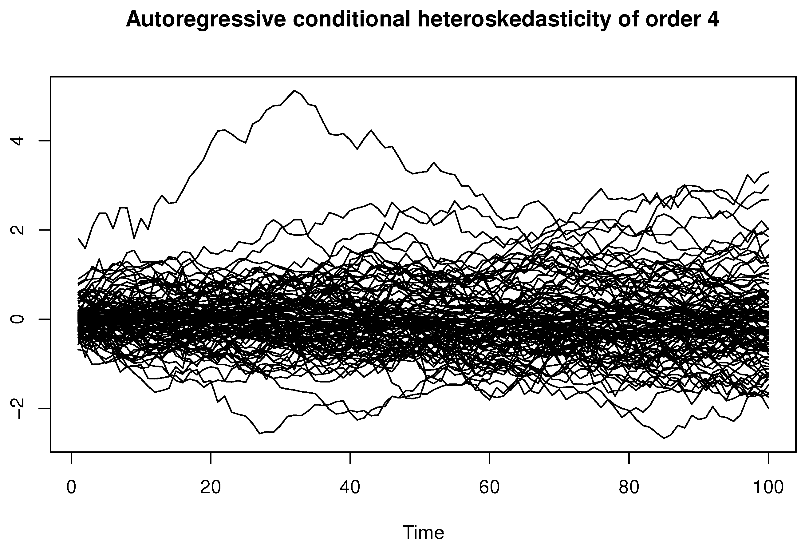
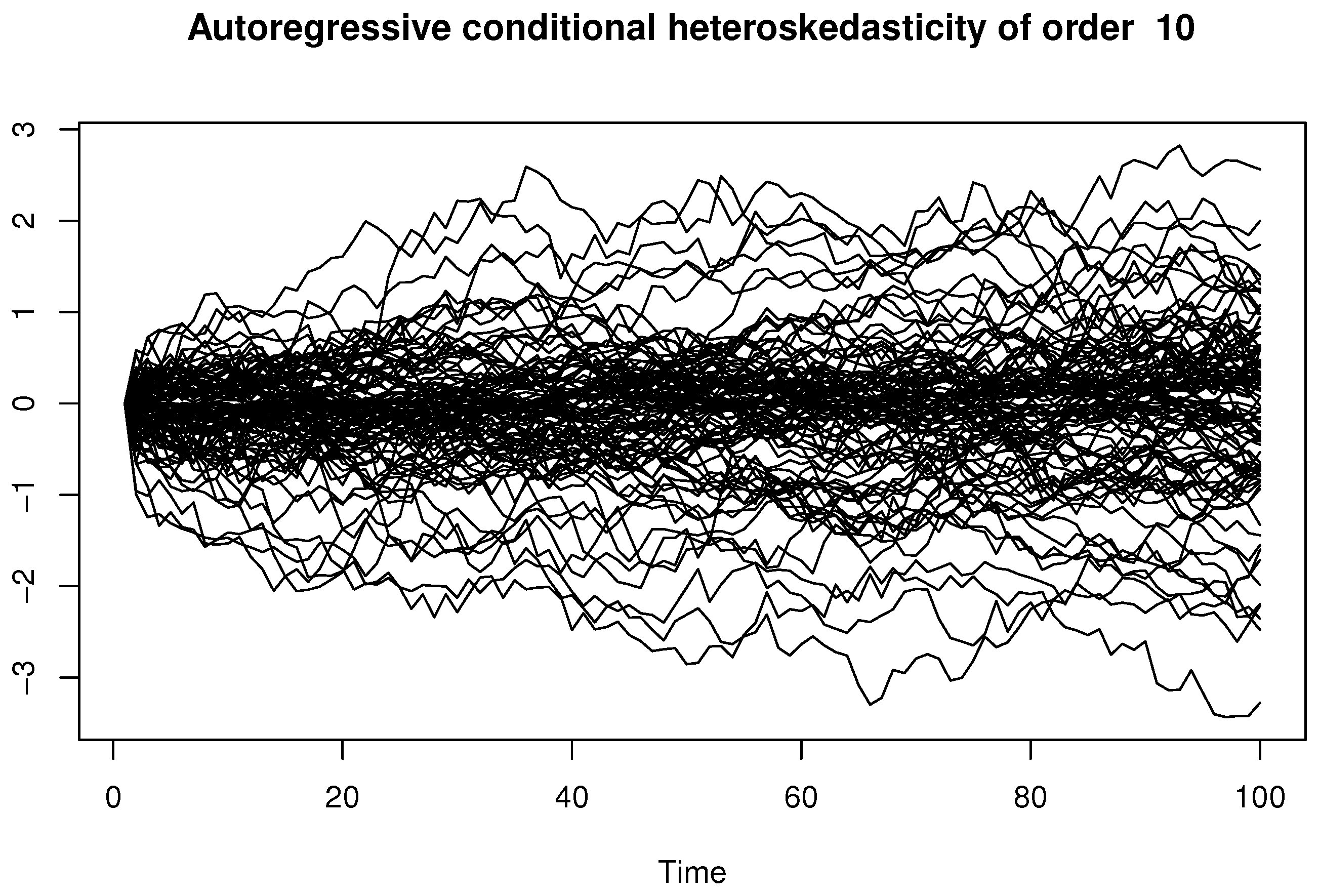
  27. Engle, R.F. Autoregressive conditional heteroskedasticity with estimates of the variance of U.K. inflation. Econometrica 1982, 50, 987–1007. [Google Scholar] [CrossRef]
  28. Jones, D.A. Nonlinear autoregressive processes. Proc. Roy. Soc. A 1978, 360, 71–95. [Google Scholar]
  29. Bollerslev, T. General autoregressive conditional heteroskedasticity. J. Econom. 1986, 31, 307–327. [Google Scholar] [CrossRef]
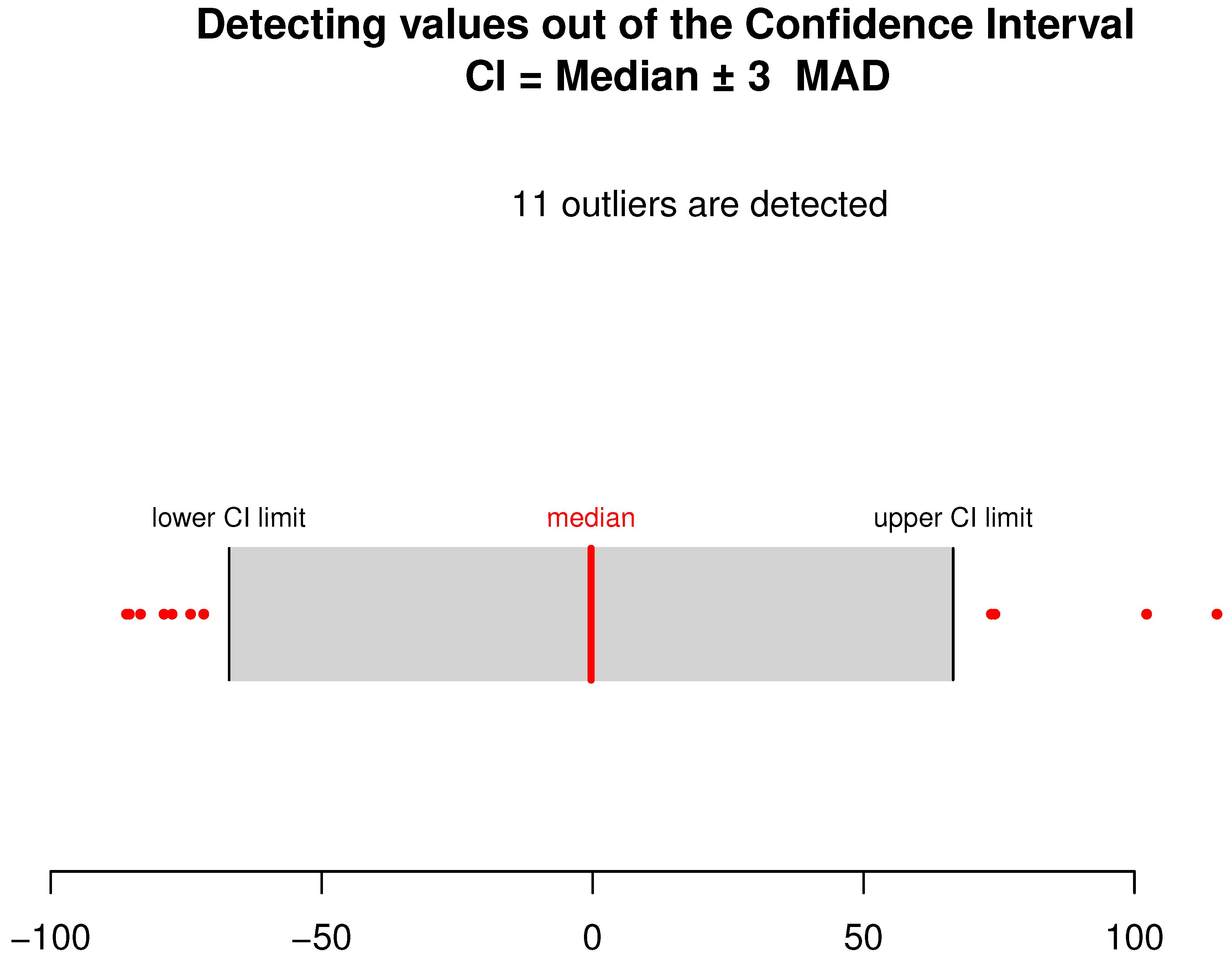
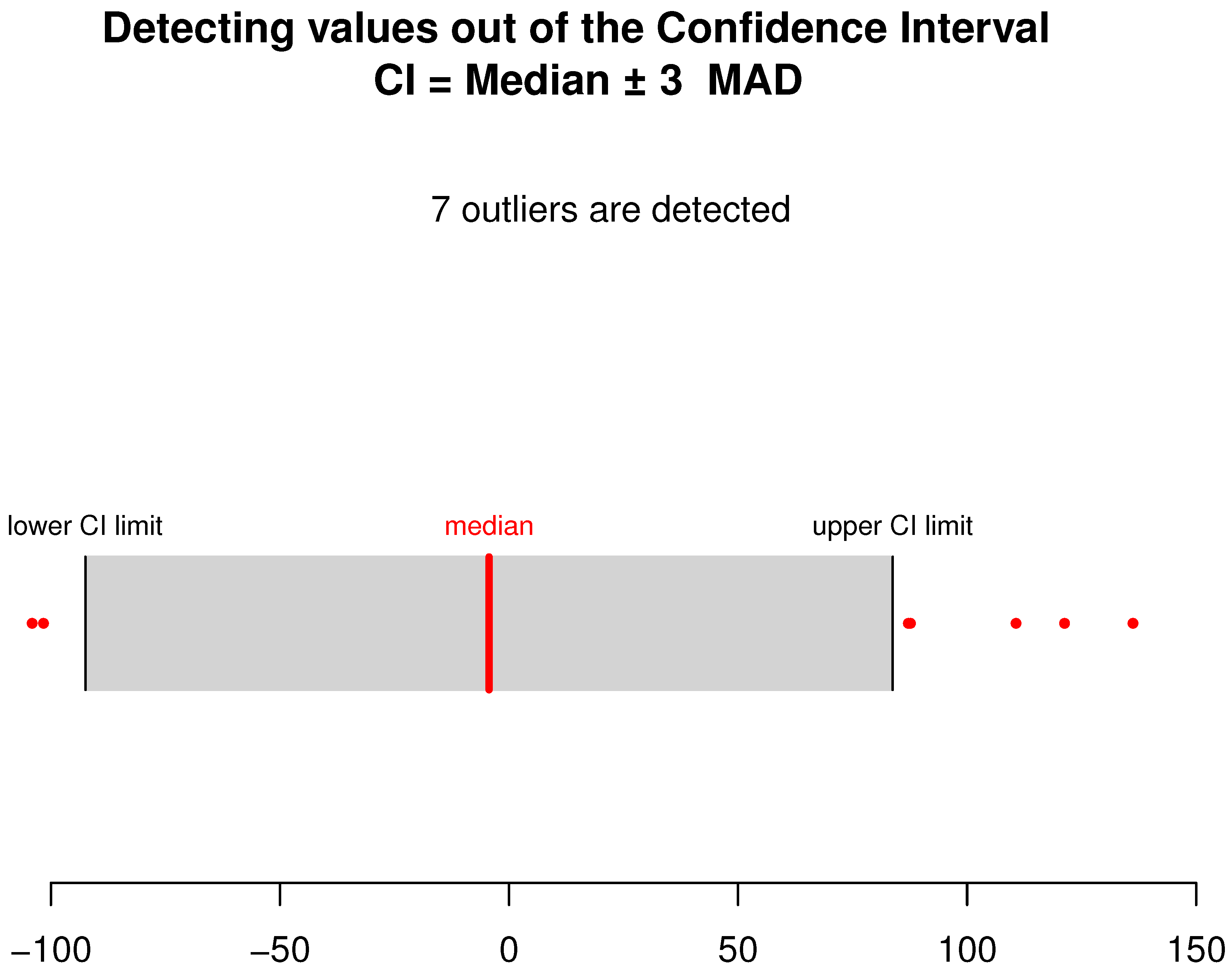
  30. Leys, C.; Ley, C.; Klein, O.; Bernard, P.; Licata, L. Detecting outliers: Do not use standard deviation around the mean, use absolute deviation around the median. J. Exp. Soc. Psychol. 2013, 49, 764–766. [Google Scholar] [CrossRef]
  31. Febrero, M.; Galeano, P.; González-Manteiga, W. Outlier detection in functional data by depth measures with application to identify abnormal NOx levels. Environmetrics 2008, 19, 331–345. [Google Scholar] [CrossRef]
  32. Azzi, A.; Belguerna, A.; Laksaci, A.; Rachdi, M. The scalar-on-function modal regression for functional time series data. J. Nonparametric Stat. 2024, 36, 503–526. [Google Scholar] [CrossRef]
Figure 1. A sample of 100 curves from FARCH(1).
Symmetry 17 00460 g001
Figure 2. A sample of 100 curves from FARCH(4).
Symmetry 17 00460 g002
Figure 3. A sample of 100 curves from FARCH(10).
Symmetry 17 00460 g003
Figure 4. The umber of outliers detected using the MAD-test. The outliers are displayed in red dots.
Symmetry 17 00460 g004
Figure 5. The number of outliers detected using the MAD test. The outliers are displayed in red dots.
Symmetry 17 00460 g005
Figure 6. The number of outliers detected using the MAD test. The outliers are displayed in red dots.
Symmetry 17 00460 g006
Figure 7. A sample of curves and the number of outlier curves.
Symmetry 17 00460 g007
Figure 8. The prediction with the robust mode M d τ ^ with outliers. The true values on black line and the predicted on the red line.
Symmetry 17 00460 g008
Figure 9. The prediction with the standard mode M d τ ˜ with outliers.The true values on black line and the predicted on the red line.
Symmetry 17 00460 g009
Figure 10. The prediction with the robust mode M d τ ^ without outliers. The true values on black line and the predicted on the red line.
Symmetry 17 00460 g010
Figure 11. The prediction with the standard mode M d τ ˜ without outliers. The true values on black line and the predicted on the red line.
Symmetry 17 00460 g011
Table 1. MAE results.
The White Noise DistributionnpOutliers Case MAE ( Md ˜ ) MAE ( Md ^ )
Laplace distribution501with outliers2.431.37
1without outliers1.060.51
4with outliers7.922.29
4without outliers1.410.39
10with outliers7.822.92
10without outliers1.950.52
1001with outliers2.361.29
1without outliers0.980.43
4with outliers7.612.17
4without outliers1.320.28
10with outliers7.662.84
10without outliers1.890.39
2501with outliers2.171.07
1without outliers0.840.32
4with outliers7.432.06
4without outliers1.110.12
10with outliers7.322.52
10without outliers1.720.25
Weibull distribution501with outliers4.542.95
1without outliers1.810.77
4with outliers4.823.23
4without outliers2.431.03
10with outliers5.913.48
10without outliers2.461.05
1001with outliers4.322.88
1without outliers1.630.69
4with outliers4.533.02
4without outliers2.010.85
10with outliers5.783.34
10without outliers2.260.92
2501with outliers4.142.63
1without outliers1.320.43
4with outliers4.252.98
4without outliers1.930.71
10with outliers5.493.11
10without outliers2.010.74
Log-normal distribution501with outliers6.531.32
1without outliers2.500.79
4with outliers5.422.54
4without outliers2.621.12
10with outliers6.612.66
10without outliers3.081.48
1001with outliers 26.361.19
1without outliers2.040.67
4with outliers5.132.33
4without outliers2.390.98
10with outliers6.442.59
10without outliers2.951.23
2501with outliers 26.111.02
1without outliers1.820.51
4with outliers5.022.07
4without outliers2.140.71
10with outliers6.362.28
10without outliers2.771.09
Disclaimer/Publisher’s Note: The statements, opinions and data contained in all publications are solely those of the individual author(s) and contributor(s) and not of MDPI and/or the editor(s). MDPI and/or the editor(s) disclaim responsibility for any injury to people or property resulting from any ideas, methods, instructions or products referred to in the content.

