Fractional Order Curves

Abstract

This paper continues the subject of symmetry breaking of fractional-order maps, previously addressed by one of the authors. Several known planar classes of curves of integer order are considered and transformed into their fractional order. Several known planar classes of curves of integer order are considered and transformed into their fractional order. For this purpose, the Grunwald–Letnikov numerical scheme is used. It is shown numerically that the aesthetic appeal of most of the considered curves of integer order is broken when the curves are transformed into fractional-order variants. The considered curves are defined by parametric representation, Cartesian representation, and iterated function systems. To facilitate the numerical implementation, most of the curves are considered under their affine function representation. In this way, the utilized iterative algorithm can be easily followed. Besides histograms, the entropy of a curve, a useful numerical tool to unveil the characteristics of the obtained fractional-order curves and to compare them with their integer-order counterparts, is used. A Matlab code is presented that can be easily modified to run for all considered curves.

Beauty is the first test. There is no permanent place in the world for ugly mathematics (Jonathan Borwein and David Bailey 2008 [1])

1. Introduction

To paraphrase the words of Jonathan Borwein and David Bailey [1], even fractional-order (FO) derivatives are generalizations of integer-order differentiation, providing a powerful tool for modeling complex systems with memory effects and hereditary properties. The beauty of the symmetries found in integer-order (IO) systems can be affected by the FO approach, as is proved numerically in this paper. The main motivation of this article is to draw attention to the fact that, although fractional-order calculus is becoming increasingly used in modeling some systems, the maintenance of symmetry can be affected (see [2], where it is shown that Caputo’s fractional-order discrete maps may lose their symmetries).

The history of non-integer order derivatives dates back to the beginning of the theory of differential calculus in 1695. On the other side, the development of the theory of fractional calculus, which is useful in engineering and mathematics and helpful for scientists and researchers working with real-life applications, starts with the work of Euler, Liouville, Riemann, and Letnikov (see [3,4]). Basic aspects of the theory of fractional differential equations can be found in [5], and for a review of definitions of fractional derivatives and other operators, see [6].

Fractional difference equations have received increasing attention recently, with one of the first definitions of a fractional difference operator being proposed in 1974 [5]. However, there are still a few works in the field of the theory of fractional finite difference equations. Problems related to Caputo-like discrete fractional differences can be found in [7], while initial value problems of fractional order are studied in [8]. Stability aspects related to fractional differences can be found in [9,10]. Some applications can be found in [11,12,13]. A comprehensive treatment of discrete fractional calculus can be found in [14]

Another widely used operator is the Grünwald–Letnikov (GL) fractional difference operator [15,16,17].

As known, simple plane curves are nonintersecting, such as space-filling curves, while not simple plane curves intersect themselves. Both simple and not simple plane curves can be closed (such as circles, epycicloids), or not closed (such as lines, parabolas, and hyperbolas). Curves that are interesting for some reason and whose properties have therefore been investigated are called “special curves” [18], such as the epicycloid considered in this paper. Usually, the curves are given in Cartesian form, polar form, or parametric form.

The aim of this paper is not to present some new insights into the curves theory, which are extremely well known and can be found in many existing works, but to show numerically that some plane patterns generated by diverse two-dimensional curves, transformed and drawn as FO plane curves, may lose their symmetry. For this purpose, the GL numerical scheme is considered. The manuscript is focused on the Preliminaries Section, where there is the utilized GL scheme and its boundedness property; the utilized algorithm, the entropy used, and the studied curves are presented; finally, there is the Section of drawing curves of FO and the Conclusion. The Appendix A presents the Matlab code to generate most of the presented curves of FO.

2. Preliminaries

The reasons to consider the GL scheme are the following: The considered curves are not long-term memory systems case, when Caputo’s derivative is recommended. The GL derivative can be directly defined in a discrete manner; it involves straightforward, less intensive summation formulas, and it is also recommended in the case of a relatively small fractional order $q\in (0,1)$.

2.1. Fractional-Order Grünval–Letnikov Scheme

Consider the following fractional difference initial value problem in the GL sense

$$\left\{\begin{array}{c}{n-L}^{{\Delta }_n^q}u\left(n\right)=f\left(u\left(n-1\right)\right),n\in {\mathbb{N}}_1,\hfill \\ u\left(0\right)=u_0.\hfill \end{array}\right.$$

(1)

Here $0<q<1$, $f:\mathbb{R}\to \mathbb{R}$, $u_0\in \mathbb{R}$, and ${n-L}^{{\Delta }_n^q}$ denotes the $q^{\mathrm{th}}$-order GL delta fractional difference operator with fixed memory length $L\in {\mathbb{N}}_1$ [19].

The Equation (1) is considered as a qth order difference equation, with $0<q<1$, because it can be treated as a fractional analogue of the classical first-order difference equation, which represents many discrete dynamical systems in the real world. We know that

$$\begin{array}{cc}\hfill {n-L}^{{\Delta }_n^q}u\left(n\right)& =\sum _{k=0}^L{(-1)}^k\left({\displaystyle \genfrac{}{}{0pt}{}{q}{k}}\right)u(n-k)\hfill \\ & ={\displaystyle \frac{1}{\Gamma (-q)}}\sum _{k=0}^L{\displaystyle \frac{\Gamma (k-q)}{\Gamma (k+1)}}u(n-k)\hfill \\ & =u\left(n\right)+{\displaystyle \frac{1}{\Gamma (-q)}}\sum _{k=1}^L{\displaystyle \frac{\Gamma (k-q)}{\Gamma (k+1)}}u(n-k),\hfill \end{array}$$

for $n\in {\mathbb{N}}_1$. Then, from (1), we obtain the numerical form, utilized in this paper as

$$u\left(n\right)=f\left(u\left(n-1\right)\right)-{\displaystyle \frac{1}{\Gamma (-q)}}\sum _{k=1}^L{\displaystyle \frac{\Gamma (k-q)}{\Gamma (k+1)}}u(n-k),n\in {\mathbb{N}}_L,$$

(2)

where the Gamma function $\Gamma (.)$ is

$$\Gamma \left(z\right)={\int }_0^{\infty }{e}^{-t}{t}^{z-1}dt$$

for $\Re \left(z\right)>0$.

The GL operator used in this paper is one of the popular difference operators that have been defined in discrete fractional calculus. This operator can be considered as the discrete version of the GL fractional derivative. The GL numerical scheme reproduces the qualitatively right behavior of the solution.

Assumption (A):  ${\displaystyle \left|f\left(\xi \right)\right|\le M,\xi \in \mathbb{R}}$.

Next the following solutions asymptotic behaviour results are presented

Lemma 1.

For $L=1$, the solution u of (2) verifies

$${\displaystyle u\to \frac{M}{1-q}\mathrm{as}n\to \infty .}$$

Proof.  

If $L=1$, we have the following first-order nonlinear difference equation

$$u\left(n\right)-qu(n-1)=f\left(u\left(n-1\right)\right),n\in {\mathbb{N}}_1,$$

whose equivalent form is given by

$$u\left(n\right)=u_0{q}^n+\sum _{k=1}^n{q}^{n-k}f\left(u\left(k-1\right)\right),n\in {\mathbb{N}}_1.$$

(3)

Assume that (A) holds. Then, for $n\in {\mathbb{N}}_1$,

$$\begin{array}{cc}\hfill \left|u\left(n\right)\right|& =\left|u_0{q}^n+\sum _{k=1}^n{q}^{n-k}f\left(u\left(k-1\right)\right)\right|\hfill \\ & \le \left|u_0\right|q^n+\left|\sum _{k=1}^n{q}^{n-k}f\left(u\left(k-1\right)\right)\right|\hfill \\ & \le \left|u_0\right|q^n+\sum _{k=1}^n{q}^{n-k}\left|f\left(u\left(k-1\right)\right)\right|\hfill \\ & \le \left|u_0\right|q^n+M\sum _{k=1}^n{q}^{n-k}\hfill \\ & =\left|u_0\right|q^n+M\left[{\displaystyle \frac{1-q^n}{1-q}}\right].\hfill \end{array}$$

Clearly, ${\displaystyle u\to \frac{M}{1-q}}$ as $n\to \infty$.    □

Lemma 2.

For $L=2$, ${\displaystyle u\to \frac{M}{q_1-q_2}\left[\frac{q_1}{1-q_1}+\frac{\left|q_2\right|}{1-\left|q_2\right|}\right]}$ as $n\to \infty$.

Proof.  

We have the following second-order nonlinear difference equation

$$u\left(n\right)-qu(n-1)-{\displaystyle \frac{q(1-q)}{2}}u(n-2)=f\left(u\left(n-1\right)\right),n\in {\mathbb{N}}_2,$$

whose equivalent form is given by

$$u\left(n\right)=C_1{q}_1^n+C_2{q}_2^n+{\displaystyle \frac{1}{q_1-q_2}}\sum _{k=1}^{n-1}\left[q_1^{n-k}-q_2^{n-k}\right]f\left(u\left(k\right)\right),n\in {\mathbb{N}}_1.$$

(4)

Here

$$q_1={\displaystyle \frac{q+\sqrt{2q-q^2}}{2}},q_2={\displaystyle \frac{q-\sqrt{2q-q^2}}{2}},$$

and $C_1$, $C_2$ are arbitrary constants. Clearly, $0<q_1<1$, $-1<q_2<0$ and $q_1-q_2>0$. Assume that (A) holds. Then, for $n\in {\mathbb{N}}_1$,

$$\begin{array}{cc}\hfill \left|u\left(n\right)\right|& =\left|C_1{q}_1^n+C_2{q}_2^n+{\displaystyle \frac{1}{q_1-q_2}}\sum _{k=1}^{n-1}\left[q_1^{n-k}-q_2^{n-k}\right]f\left(u\left(k\right)\right)\right|\hfill \\ & \le \left|C_1\right|q_1^n+\left|C_2\right|{\left|q_2\right|}^n+\left|{\displaystyle \frac{1}{q_1-q_2}}\sum _{k=1}^{n-1}\left[q_1^{n-k}-q_2^{n-k}\right]f\left(u\left(k\right)\right)\right|\hfill \\ & \le \left|C_1\right|q_1^n+\left|C_2\right|{\left|q_2\right|}^n+{\displaystyle \frac{1}{q_1-q_2}}\sum _{k=1}^{n-1}\left[q_1^{n-k}-q_2^{n-k}\right]\left|f\left(u\left(k\right)\right)\right|\hfill \\ & \le \left|C_1\right|q_1^n+\left|C_2\right|{\left|q_2\right|}^n+{\displaystyle \frac{M}{q_1-q_2}}\sum _{k=1}^{n-1}\left[q_1^{n-k}+{\left|q_2\right|}^{n-k}\right]\hfill \\ & =\left|C_1\right|q_1^n+\left|C_2\right|{\left|q_2\right|}^n+{\displaystyle \frac{M}{q_1-q_2}}\left[q_1\left({\displaystyle \frac{1-q_1^{n-1}}{1-q_1}}\right)+\left|q_2\right|\left({\displaystyle \frac{1-{\left|q_2\right|}^{n-1}}{1-\left|q_2\right|}}\right)\right].\hfill \end{array}$$

Clearly, for $n\to \infty$, ${\displaystyle u\to \frac{M}{q_1-q_2}\left[\frac{q_1}{1-q_1}+\frac{\left|q_2\right|}{1-\left|q_2\right|}\right]}$.    □

Remark 1.

In a similar way, we are entitled to consider that for $L\in {\mathbb{N}}_1$, u tends to a finite number as $n\to \infty$, provided (A) holds. Being defined with continuous functions on compact intervals, the considered functions verify Assumption (A).

To implement the numerical Scheme (2), for some $L\in {\mathbb{N}}_1$ and given $u\left(0\right)$, one computes the first starting values $u\left(1\right),u\left(2\right),\dots ,u(L-1)$ with one of the following relations (see Remark 3)

$$u\left(n\right)=f\left(u\left(n-1\right)\right),n=1,2,\cdots ,L-1,$$

or

$$u\left(n\right)=u(n-1)+f\left(u\right(n-1\left)\right),n=1,2,\dots ,L-1,$$

after which the scheme is applied to next points L, $L+1$, … (see Algorithm 1)

The main difference between fractional-order difference equations and ordinary difference equations lies in the order of the differences used and their ability to capture memory effects. Ordinary difference equations are the discrete counterpart of differential equations, using integer-order differences to model discrete-time systems. They describe models with integer-step evolution and are commonly used in numerical methods, control systems, and signal processing. Fractional-order difference equations extend ordinary difference equations by allowing non-integer (fractional) orders of differences, based on fractional difference operators, often the Grünwald-Letnikov, Caputo, or Riemann-Liouville formulations. They model systems with memory and hereditary properties, where the current state depends on past states. Due to their ability to model complex systems with memory, non-local interactions, and anomalous dynamics, fractional finite difference equations are useful in modeling real-world phenomena where standard integer-order models fail and have practical applications in various fields such as: engineering and physics (signal and image processing, control systems, electromagnetism); finance and economics (stock market and risk analysis, option pricing); biology and medicine (neuroscience, epidemiology); environmental and Earth sciences (groundwater flow and pollution transport, climate modeling); material science and mechanics (viscoelastic materials, fracture mechanics); computer science and artificial intelligence (machine learning, cryptography).

Algorithm 1 Algorithm for GL scheme (2)

2.2. Considered Curves and Fractals

There are several classifications of plane curves. In accordance with the purpose of this paper, we consider the following classification of the analyzed curves. The fractional-order Mandelbrot and Julia fractal sets are not considered here; they can be found in [20,21].

2.2.1. Parametric Curves

As known, a parametric equation expressing, e.g., the coordinates of a point as functions of one or several variables (parameters) is called a parametric equation. If there is a single parameter (generally $time$), the parametric equations usually express the trajectory of a moving point, which describes a curve called a parametric curve [22]. As known, these curves are described by the set of equations.

$$\begin{array}{c}x=f\left(t\right),\hfill \\ y=g\left(t\right),t\in I=[t_1,t_2],\hfill \end{array}$$

(5)

where $f,g$ are some continuous functions on I and the parameter of the curve is $t\in \mathbb{R}$ (the polar form is not considered here).

To draw a parametric curve, the algorithm presented in Algorithm 2 can be used.

Algorithm 2 Parametric curves representation

1: Input $\Delta t$, $t_1$, $t_2$ 2: for $t\leftarrow t_1$ to $t_2$ step $\Delta t$ do 3:       $x\leftarrow x\left(t\right)$ 4:       $y\leftarrow y\left(t\right)$ 5:     plot(x,y) 6: end for

In this case, the discretization required by the GL scheme can be done in the following way: instead of $x\left(t\right)$, for increasing $t:t_1,t_1+\Delta t,t_2+\Delta t,\dots$ one considers

$$x(n\Delta t),\mathrm{for}n=1,2,\dots .$$

(6)

2.2.2. Cartesian Curves

Most of the considered curves in this paper could be considered to belong to the class of curves that can be described as functions in Cartesian coordinates.

The Barnsley fern fractal, one of the basic examples of self-similar sets considered here, is not a curve. However, this fractal is presented in this paper due to its spectacularity and, especially, because it can be generated with the affine transformations used to generate the other space-filling curves.

$\left(i\right)$

Maps

Some of the most spectacular curves from this class are the partial Gaussian summations, which give rise to a beautiful family of Cornu spirals, known also as Curlicues curves (see e.g., [23,24,25,26]). Curlicues are, in the visual arts, fancy twists, or curls, composed usually of a series of concentric circles and are fractals.

$\left(ii\right)$

Space-filling curves

Usually, the space-filling curves fill a rectangular region of space. There are many variations of the space-filling curves, but the simplest version is a continuous curve that passes through every point in, usually, the unit square. Generally, they are continuous surjective functions that map the unit interval $[0,1]$ into the unit square $[0,1]\times [0,1]$. Compared to the parametric curves and some curlicues, space-filling curves may contact (or not) one another but do so without crossing (see [27]).

This kind of curve can be characterized in the metric space ${\mathbb{R}}^2$ by the fractal dimensionD (see [28]), a measure of how “complicated” a self-similar figure is, which is a real number to characterize fractal patterns or sets, greater than the topological dimension $d_T$ and less than the Euclidean dimension $d_E$ of the embedding space.

$$d_T\le D\le d_E.$$

In the plane, $d_T=1$ and $d_E=2$ and therefore, for plane fractal curves, D, could be a real number. In concrete examples, where the fractal is made by using the similarity property, the fractal dimension, D, can be calculated as the log of the number of the obtained pieces N obtained every iteration divided by the log of the magnification factor r

$$D={\displaystyle \frac{log\left(N\right)}{log\left(r\right)}}.$$

(7)

Because the space-filling curves reach every point in a region of the plane, following the generation process, it is easy to understand that $D=2$.

The curves considered here are the Hilbert curve and the Péano curve.

$\left(iii\right)$

Iterated Function Systems (IFS)

Several space-filling curves can be obtained by using affine transformations, which have the form

$$\begin{array}{c}T\left(\begin{array}{c}x\\ y\end{array}\right)=scale·A\left(\begin{array}{c}x\\ y\end{array}\right)+scale·\left(\begin{array}{c}t{r}_x\\ t{r}_y\end{array}\right),\end{array}$$

(8)

where A is a $2\times 2$ real matrix representing linear transformations and $tr={(t{r}_x,t{r}_y)}^t$ is the translation matrix. For a unitary representation of functions for all considered systems, the scaling scalar $scale$ is extracted as a common factor of the matrices A and $tr$. To note that affine functions are composed of a linear function with a translation, but generally, there is also a possible separate transformation: the rotation (which is not part of an affine transformation by itself). The plane rotation matrix with the angle $\alpha$ has the form

$$R\left(\alpha \right)=\left(\begin{array}{c}cos\alpha -sin\alpha \\ sin\alpha cos\alpha \end{array}\right),$$

(9)

and to rotate the point $u={(x,y)}^t$ with an angle $\alpha$, one calculates $Ru$.

The most famous fractal from the class of IFS, which is a set of points generated randomly, but it is not a curve, is the Barnsley fern.

For the considered curves in this section, the operators T in (8), given by matrices A, $tr$, and $scale$, are presented in

Table 1. The elements of the affine functions utilized in simulations.

Curve	A	tr	$\mathit{Scale}/\mathit{Probability}$
Hilbert	$\left(\begin{array}{cc}0& 1\\ 1& 0\end{array}\right)$   $\left(\begin{array}{cc}1& 0\\ 0& 1\end{array}\right)$   $\left(\begin{array}{cc}1& 0\\ 0& 1\end{array}\right)$ $\left(\begin{array}{cc}0& -1\\ -1& 0\end{array}\right)$	$\left(\begin{array}{c}-{\displaystyle \frac{1}{2}}\\ -{\displaystyle \frac{1}{2}}\end{array}\right)$  $\left(\begin{array}{c}-{\displaystyle \frac{1}{2}}\\ {\displaystyle \frac{1}{2}}\end{array}\right)$   $\left(\begin{array}{c}{\displaystyle \frac{1}{2}}\\ {\displaystyle \frac{1}{2}}\end{array}\right)$   $\left(\begin{array}{c}{\displaystyle \frac{1}{2}}\\ -{\displaystyle \frac{1}{2}}\end{array}\right)$	$scale={\displaystyle \frac{1}{2}}$
Peano	$\left(\begin{array}{cc}1& 0\\ 0& 1\end{array}\right)$  $\left(\begin{array}{cc}1& 0\\ 0& -1\end{array}\right)$  $\left(\begin{array}{cc}1& 0\\ 0& 1\end{array}\right)$  $\left(\begin{array}{cc}-1& 0\\ 0& 1\end{array}\right)$  $\left(\begin{array}{cc}-1& 0\\ 0& -1\end{array}\right)$  $\left(\begin{array}{cc}-1& 0\\ 0& 1\end{array}\right)$  $\left(\begin{array}{cc}1& 0\\ 0& 1\end{array}\right)$  $\left(\begin{array}{cc}1& 0\\ 0& -1\end{array}\right)$  $\left(\begin{array}{cc}1& 0\\ 0& 1\end{array}\right)$	$\left(\begin{array}{c}-1\\ -1\end{array}\right)$  $\left(\begin{array}{c}0\\ -1\end{array}\right)$  $\left(\begin{array}{c}1\\ -1\end{array}\right)$  $\left(\begin{array}{c}1\\ 0\end{array}\right)$  $\left(\begin{array}{c}0\\ 0\end{array}\right)$  $\left(\begin{array}{c}-1\\ 0\end{array}\right)$  $\left(\begin{array}{c}-1\\ 1\end{array}\right)$  $\left(\begin{array}{c}0\\ 1\end{array}\right)$  $\left(\begin{array}{c}1\\ 1\end{array}\right)$	$scale={\displaystyle \frac{1}{3}}$
Koch	$\left(\begin{array}{cc}1& 0\\ 0& 1\end{array}\right)$  $\left(\begin{array}{cc}{\displaystyle \frac{1}{2}}& -{\displaystyle \frac{\sqrt{3}}{2}}\\ {\displaystyle \frac{\sqrt{3}}{2}}& {\displaystyle \frac{1}{2}}\end{array}\right)$  $\left(\begin{array}{cc}{\displaystyle \frac{1}{2}}& {\displaystyle \frac{\sqrt{3}}{2}}\\ -{\displaystyle \frac{\sqrt{3}}{2}}& {\displaystyle \frac{1}{2}}\end{array}\right)$  $\left(\begin{array}{cc}1& 0\\ 0& 1\end{array}\right)$	$\left(\begin{array}{c}0\\ 0\end{array}\right)$  $\left(\begin{array}{c}1\\ 0\end{array}\right)$  $\left(\begin{array}{c}{\displaystyle \frac{1}{2}}\\ {\displaystyle \frac{\sqrt{3}}{2}}\end{array}\right)$ $\left(\begin{array}{c}2\\ 0\end{array}\right)$	$scale={\displaystyle \frac{1}{3}}$
Fern	$\left(\begin{array}{cc}0& 0\\ 0& 0.16\end{array}\right)$  $\left(\begin{array}{cc}0.85& 0.04\\ -0.04& 0.85\end{array}\right)$  $\left(\begin{array}{cc}0.20& -0.26\\ 0.23& 0.22\end{array}\right)$  $\left(\begin{array}{cc}-0.15& 0.28\\ 0.26& 0.24\end{array}\right)$	$\left(\begin{array}{c}0\\ 0\end{array}\right)$  $\left(\begin{array}{c}0\\ 1.60\end{array}\right)$  $\left(\begin{array}{c}0\\ 1.60\end{array}\right)$ $\left(\begin{array}{c}0\\ 0.44\end{array}\right)$	$p=0.01$   $p=0.85$   $p=0.07$   $p=0.07$

.

The space-filling curves and IFS curves are usually generated recursively; additionally, some of them can be constructed as L-systems (Lindenmayer systems) via a type of formal grammar [29]. Also, recursive turtle programs can be used to generate such curves. For a recursive generation of the IO Hilbert curve, see [30], while for the IO Péano curve, see [31].

Remark 2.

These space-filling curves and IFS systems can be programmed via affine transformations (see e.g., [32]), which can be simply implemented in the GL scheme (2). Therefore, in this paper, for the construction of the IO and FO space-filling curves, this approach is used.

2.3. Entropy of a Curve

One of the tools utilized in this paper is entropy. The concept of information entropy has been introduced by Claude Shannon in 1948 [33] and is also referred to as Shannon entropy. The entropy of a curve is, roughly speaking, 0 when the curve is a straight line and increases when the curve becomes more “jagged”; it is based on the distribution of its values. Thus, the entropy indicator clearly depends on the irregularity of the curve. Entropy can be used to study the time evolution of a curve. The theory of thermodynamics of a curve was born in 1983 once with the pioneering work of Mèdes France [34] (see also [35]). In analogy with Shannon’s measure of entropy, the entropy of a curve can be defined as

$$H(\Gamma )=-\sum _{n=1}^{\infty }{P}_n{log}_2{P}_n,$$

where $P_n$ is the probability for a line to intersect a plane curve in n points (see [36]), the sum being truncated. In this paper, this indicator is shown to be useful to unveil the role of the fractional order q in the shape of the obtained FO curve.

3. Drawing the Patterns of the FO Curves

A computer program to generate such curves is either recursive (when an entity calls itself) or iterative (when there is a loop or repetition). In this paper, the iterative way is chosen, and a Matlab code is presented in the Appendix A. The program can be easily adapted to generate all considered Cartesian curves. Because the influence of L on results is not significant, L is considered $L\in \{3,4,5\}$, the only necessary condition being $N>L$.

Notation The curves of IO are denoted $\Gamma$, and the FO curves, generated with the GL scheme, for a fixed fractional order q, are denoted ${\Gamma }_q$.

Remark 3.

The affine representation of the curves, like the Hilbert curve, Péano curve, Koch curve, Dragon curve, and Barnsley fern, is obtained through an iterative additive update (see the relation (8)), i.e., it can be modeled by the following general form:

$$u\left(n\right)=Au(n-1)+b,n=1,2,\dots$$

(10)

In the Algorithm 1, $f\left(u\right(n-1\left)\right):=Au(n-1)+b$.

The curlicue curves (16) can also be defined as additive update iteration:

$$u\left(n\right)=u(n-1)+f\left(u\right(n-1\left)\right),n=1,2,\dots$$

(11)

On the other side, the parametric considered curves are defined as iterative multiplicative (functional) updates, i.e.,

$$u\left(n\right)=f\left(u\right(n-1\left)\right)n=1,2,\dots$$

(12)

3.1. FO Parametric Curves

Two parametric curves are considered next.

3.1.1. Surface-Like Curve

Most spectacular parametric curves are modeled with trigonometric functions. Let the curve described by the following equations.

$$\begin{array}{cc}\hfill x\left(t\right)& =0.99cos\left(0.99t\right)+2.107sin\left(3.01t\right)\hfill \\ \hfill y\left(t\right)& =-1.01sin\left(1.01t\right)+1.503cos\left(15.03t\right),\mathrm{for}t=0,\Delta t,2\Delta t,\dots \hfill \end{array}$$

(13)

where $\Delta t\in {\mathbb{R}}_{+}$. The equations of IO (13) generate the surface-like curve $\Gamma$ in Figure 1a. Following the transformation presented in Section 2.2.1, $x\left(t\right)$ and $y\left(t\right)$ are transformed as follows:

$$\begin{array}{cc}\hfill x\left(n\right)& =0.99cos(0.99n\Delta t)+2.107sin(3.01n\Delta t)\hfill \\ \hfill y\left(n\right)& =-1.01sin(1.01n\Delta t)+1.503cos(15.03n\Delta t),\mathrm{for}n=0,1,\dots \hfill \end{array}$$

(14)

which can be implemented in the GL scheme (2). The obtained FO curve, for $q=0.5$, $L=5$, and with $\Delta t=1e-2$, is presented in Figure 1b. Histograms (Figure 1c,d, respectively) indicate some differences between $\Gamma$ and ${\Gamma }_{0.5}$, but, as can be seen, except for their size, their shapes look similar. On the other side, the entropy of ${\Gamma }_{0.5}$ (Figure 1c reveals a higher irregularity of ${\Gamma }_{0.5}$ compared to $\Gamma$, a fact that seems counterintuitive since the curves apparently look similar and have the same shape. As expected, $H_{min}=1.959$, which is reached for $q\to 0$ and $q\to 1$, corresponds to $\Gamma$, and $H_{max}=2.287$ is attained at $q=0.6$. From a computationally point of view, software like Matlab can deal with the singularity of $\Gamma \left(0\right)$.

Symmetries: The parametric curve of IO does not exhibit symmetry with respect to the x-axis, y-axis, or origin (see Remark 6 (i)).

3.1.2. Epycicloid

Another spectacular curve, the epicycloid (also called hypercycloid) of IO, $\Gamma$ is presented in Figure 2a (red plot) for $a=2.1$, $b=1$. Its transformed equations are

$$\begin{array}{c}\hfill x\left(n\right)=(a+b)cos(n\Delta t)-bcos\left(\right(a/b+1)n\Delta t)\\ \hfill y\left(n\right)=(a+b)sin(n\Delta t)-bsin\left(\right(a/b+1)n\Delta t),n0,1,\dots ,\end{array}$$

(15)

The FO variant for $q=0.5$ is superimposed over the IO variant $\Gamma$ (Figure 2a (blue plot). Again, as for the curve (14), the only influence of the fractional order q consists in the size in the space $(x,y)$. The entropy is presented in Figure 2b with $H_{min}=2.832$ and $H_{max}=2.62$ at $q=0.55$. Despite the fact that apparently there are no differences between the two curves, their histograms, Figure 2c,d, indicate some smaller differences.

Symmetries: The IO curve has rotational symmetry about the center; it has mirror symmetry against multiple axes passing through the center, i.e., it remains unchanged when reflected along these axes (see Remark 6 ($ii$)).

Remark 4.

The fractional order can refine the peaks of a curve, but the effect depends on the specific system, the nature of the fractional derivative, and the chosen fractional order. Thus, while generally the peaks broaden and shift under the effect of fractional order, probably due to the particular discretization (6), only peak shifting has been observed (see the case of the curve (15)). A similar phenomenon appears in the FO curlicues in Figure 3e,f.

3.2. FO Curlicues

Some of these curves considered in this paper can be generated by iterating the complex map $e^{i2\pi f\left(n\right)}$, $n=0,1,\dots$, which, in the cartesian form reads [25]

$$\begin{array}{cc}\hfill x(n+1)& =x\left(n\right)+cos\left(2\pi f\right(n\left)\right),n=0,1,\dots \hfill \\ \hfill y(n+1)& =y\left(n\right)+sin\left(2\pi f\right(n\left)\right)\hfill \end{array}$$

(16)

where $f\left(n\right)=n^m/p$, for different positive integers m and p.

In Figure 3, several cases are considered. In Figure 3a–c, three are curlicues of IO for $m=2$, $p=1000$, $m=3$, $p=1002$, and $m=3$, $p=1013$, respectively. In Figure 3d–i, FO curlicues are presented. In Figure 3d–f, the FO curlicues are represented, a variant of their IO counterparts in Figure 3a–c, q being set at $0.01$, while in Figure 3g, $q=0.1$. As can be seen, the influence of q in the shape of curves is important. Histograms in Figure 3h, for $m=3$ and $p=1013$ (top: the IO; bottom: FO), also underline this difference. The entropy $H_{min}=1380$, while $H_{max}=3.750$ at $q=0.7$.

Symmetries: Curlicue curves exhibit quasi-symmetry (not fully symmetric) and, generally, do not have exact reflectional or rotational symmetry and could preserve the symmetry of f. Based on the simulation results, one can conclude that the FO approach affects the curlicue symmetries.

3.3. Space-Filling Curves

The space-filling curves presented next are the Hilbert curve and Péano curve.

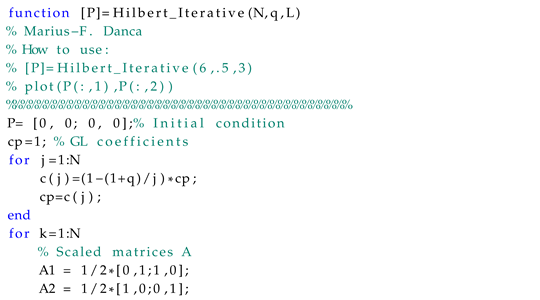
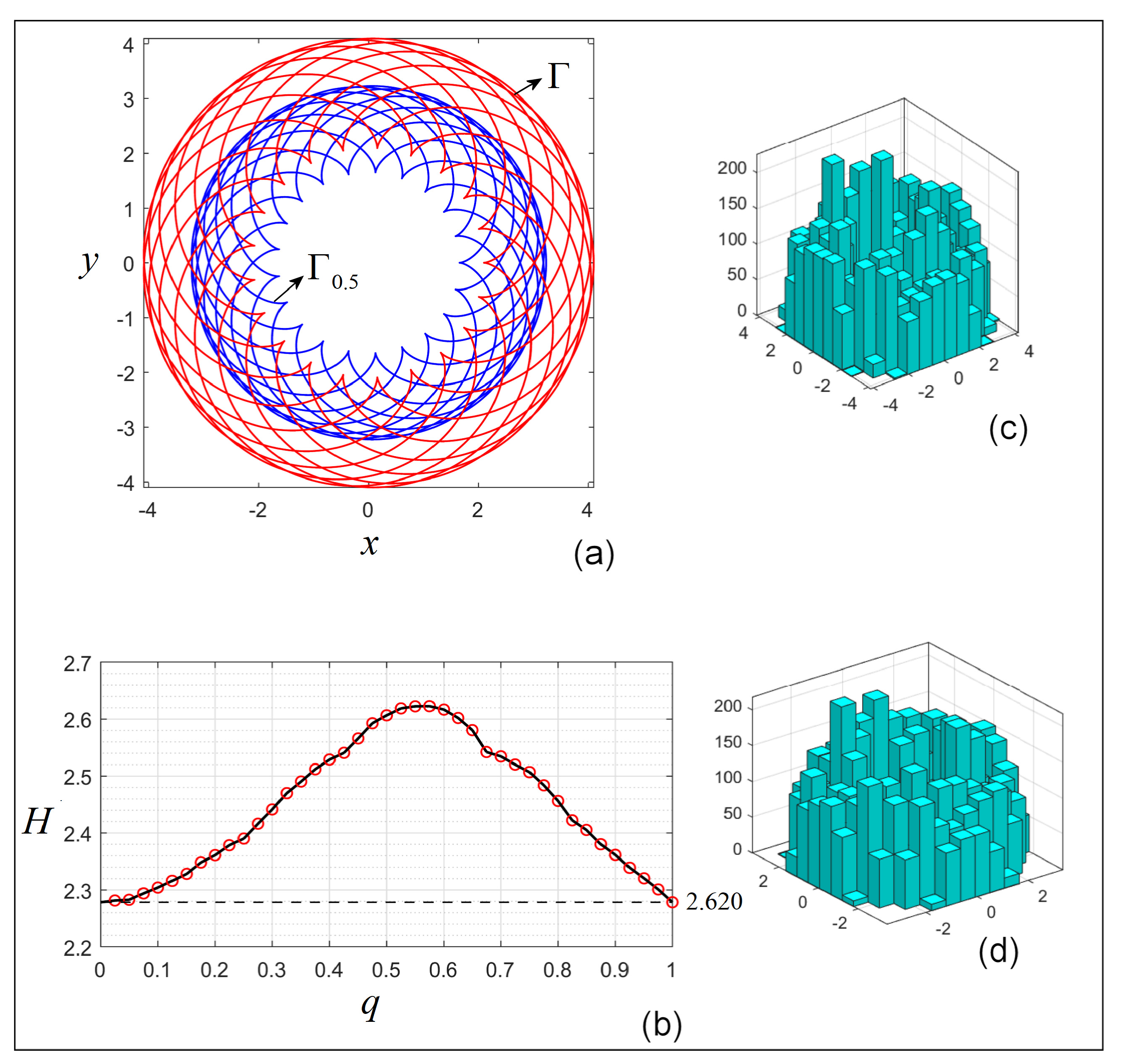
3.3.1. Hilbert Curve

The Hilbert curve [37], a self-similar and recursive curve, is constructed as a limit of piecewise linear (affine) curves generally embedded into the square $[0,1]\times [0,1]$. The initial shape is a U-shaped generator, which has four possible orientations by scaling, rotating, and translating in each iteration (Figure 4a). Note that line segments linking the shapes U together (red plot) are used. At each stage, the side length of the square is halved. The four affine functions defining the curves, applied in the 4 quadrants (see Figure 4a,b), are given in Table 1 (The Matlab code in the Appendix A is designed to generate Hilbert curves).

On the top of Figure 3a–c are the results for the IO case, while for the FO case, the results are presented at the bottom of the figure (Figure 3d–h). The perfect order in the shape of IO is revealed, beside Figure 4b (for $N=6$, when the graphical result is still clear), by the histogram in Figure 4c. In the FO case, in Figure 3d, the curves of order $N=3$ and 4 for $q=0.12$ are presented. The non-crossing limit iteration for $q=0.12$ was $N=6$ (Figure 4e). As expected, for higher q, $q=0.75$, the disorder increases, and the self-crossing phenomenon appears (see Figure 3f). This fact can also be deduced from the entropy evolution in Figure 3, where one can see that $H\left(0.12\right)$ is smaller than $H\left(0.75\right)$.

Symmetries: The fractal Hilbert of the IO curve presents several symmetries: self-similarity; reflection symmetry; smaller segments exhibit ${90}^{\circ }$ local rotational symmetry and are invariant under ${180}^{\circ }$ rotation (see Remark 6 (i)).

3.3.2. Péano Curve

This curve, called a “monstrous curve”, was discovered first by Péano in 1890 [38]. To note that Péano did not provide an explicit description of what his curve might look like but only defined a pair of functions for x and y coordinates inside a square for each position along a line segment. Against expectations, they are not fractals [39] and may be constructed recursively (divide-and-conquer process and exploiting self-similarity).

The Péano curve is based on a $3\times 3$ grid usually considered in the square $[0,1]\times [0,1]$. Therefore, it is more complex than the Hilbert curve, having 9 transformations applied in the circled 9 points (centers of 9 ninths of a square quarter; see Figure 5a). In Figure 5, the curve for $N=4$ iterations is presented. The FO cases, $q=0.2$ and $q=0.5$ for $N=3$, $N=4$, and $N=5$, are presented in Figure 5d,e,g, respectively. The histograms (Figure 5c,f, respectively) underline the differences between the IO and FO cases. Now, the fact that the FO curve covers less than the square considered is more obvious than for the Hilbert curve (Figure 5e,g) and indicates that the fractal dimension D is smaller than its IO variant, i.e., $D<2$. The irregularity of the FO Péano curve is unveiled by the entropy H (Figure 5h).

Symmetries: The IO Péano’s curves present self-similarity; reflection symmetry (Hilbert and Péano curves have horizontal and vertical reflection symmetry); rotational 90° symmetry (see Remark 6 (i)).

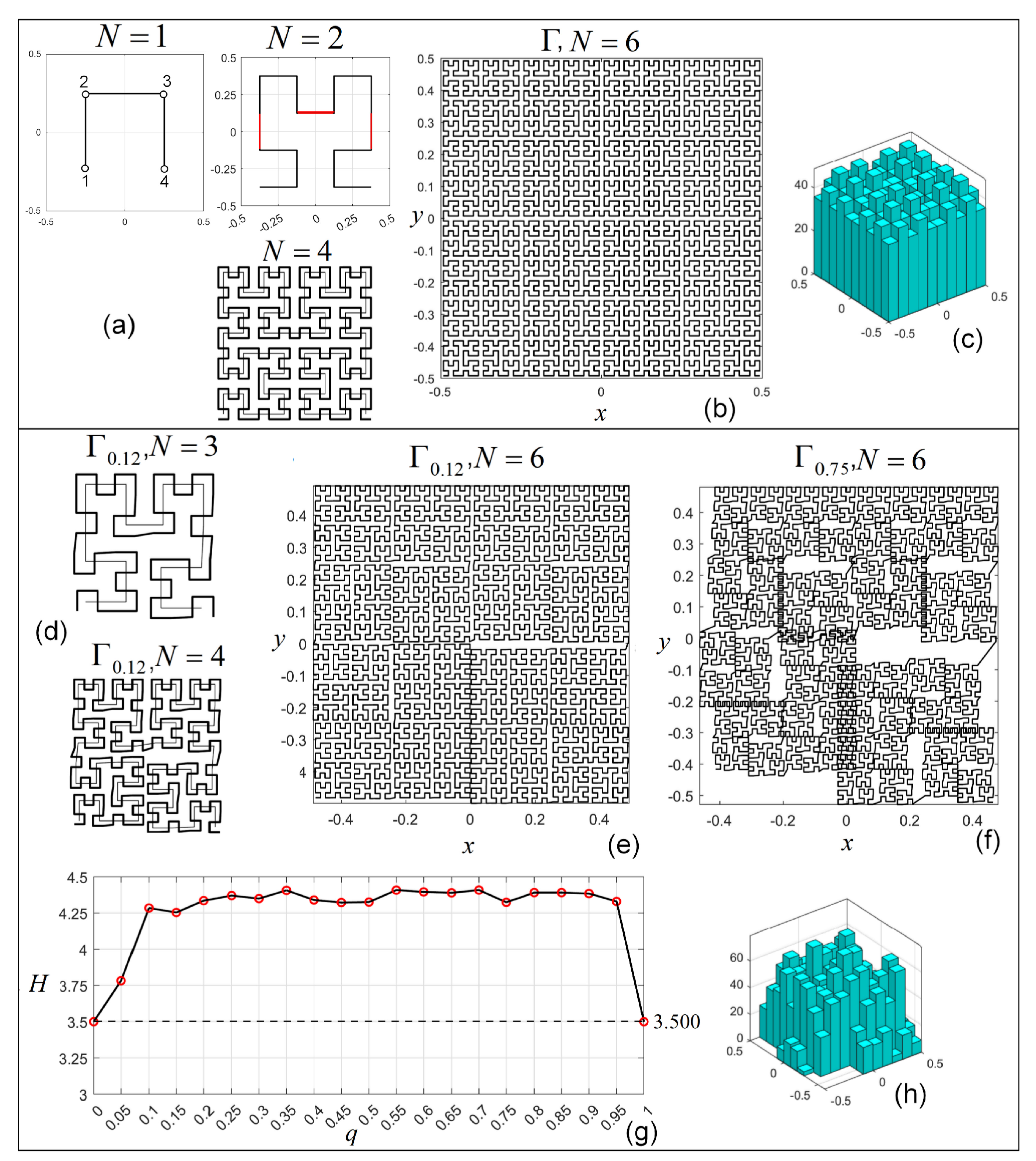
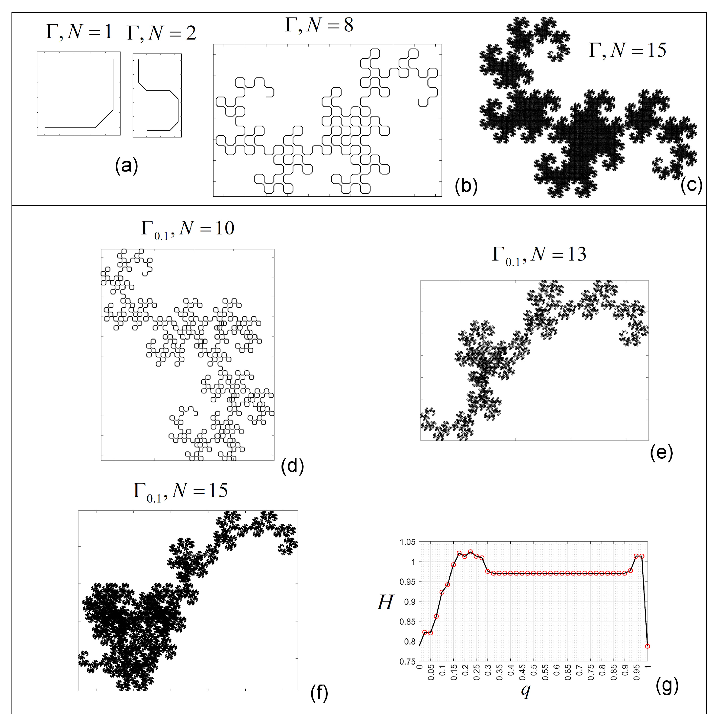
3.4. Koch Fractal Curve

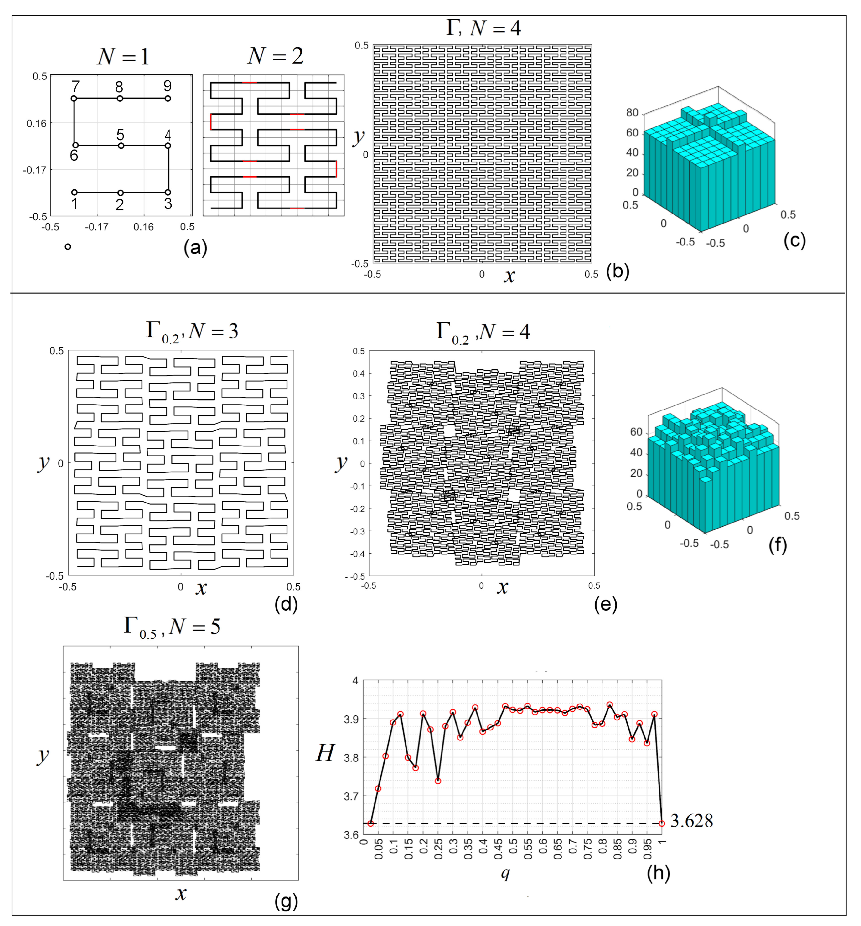
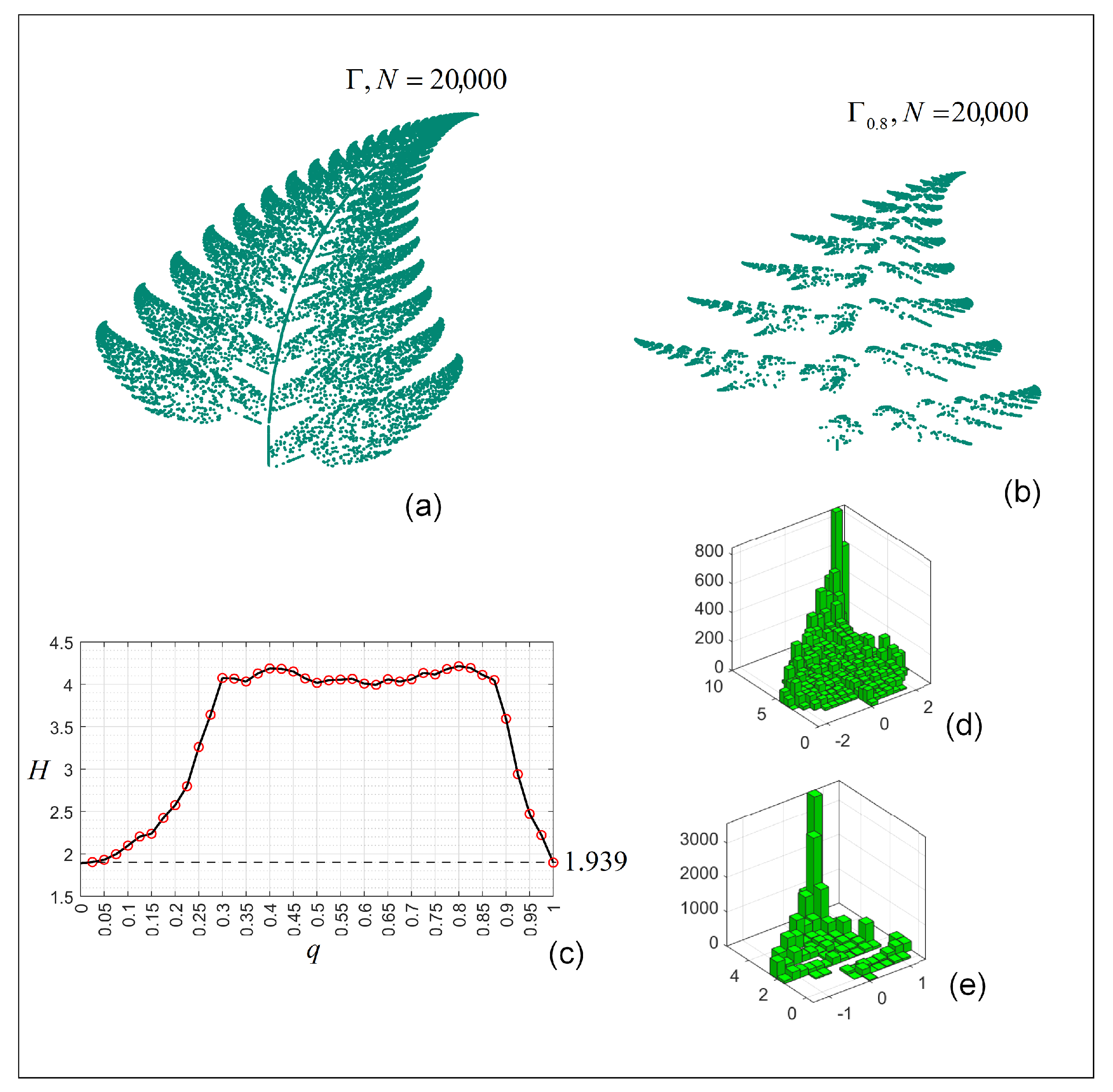
Koch fractal curves are some of the most intuitive uniform self-similar fractal curves and one of the earliest described fractals [39,40] ch. 6.

In Figure 6 are presented the IO case for $N=5$ and the generator (Figure 6a), while in Figure 6b,c,f the FO cases for $q=0.15$ and $N=2,3,5$ iterations. Histograms in Figure 6e reveal the differences between the two cases, while the irregularity of the FO curves can be viewed in the histogram as a function of q (Figure 6d).

The four transformations $T_i$, $i=1,2,3,4$ acting on the four points 1st-4th (see Figure 6) are presented in Table 1.

The Koch curve is a fractal with fractal dimension calculated with (7) is $D=log4/log\left(3\right)\approx 1.261<2$ and, therefore, it is not a space-filling curve.

Symmetries: The IO curve presents self-similarity; rotational symmetry (it has rotational symmetry of order 3 in the sense that the entire shape can be rotated by 120° or 240° without changing its shape); reflection symmetry (three axes of reflection symmetry, corresponding to the lines that pass through opposite points of its triangular structure) (see Remark 6 (i)).

For a better understanding of space-filling curve generation, see, e.g., [41,42,43].

Remark 5.

The affine functions defining the above space-filling curves are not unique.

3.5. Barnsley Fern

One of the most famous iterated function systems (IFS) is the fern, Barnsley fern (Figure 7) named after the British mathematician Michael Barnsley, who first described it in his book [43]. It is obtained with the code developed by Barnsley, which refers to the iterated function system (IFS). The four affine transformations are called only when the randomly generated probability p receives the values proposed by Barnsley (see Table 1). However, the data defining this fractal can be modified.

Symmetries: The IO curve exhibits self-similarity (see Remark 6 (i)).

3.6. FO Dragon Curve

This curve, whose name derives from its resemblance to a certain mythical creature, was described by Martin Gardner in his Scientific American column Mathematical Games in 1967 [44].

In Figure 8, the IO and FO of the dragon curve are presented. Because the path of the curve designed to avoid the tangency requires a longer set of functions, it is not represented in Table 1. As expected, the FO leads to self-crossings, even for small values of q.

Symmetries: The Dragon Curve of IO is a self-similar fractal and has two-fold rotational symmetry (180° symmetry) (see Remark 6 (i)).

Remark 6. Symmetry breaking

Notions on symmetries in mathematics, physics, and nature, as well as the historical development of symmetry concepts see, e.g., [45,46], respectively. Symmetry breaking in fractional-order maps occurs due to the memory effect and the non-local nature of fractional derivatives. Thus, unlike integer-order maps, where dynamics are determined solely by the present state, fractional-order maps incorporate past states, leading to asymmetric behavior even if the system itself appears symmetric in structure. This phenomenon affects the graphical results, even if the governing equations are symmetric. Also, the weighted sum of all past states (see (1)), leads to deviations from the expected symmetric behavior. Moreover, directional biases appear that can break symmetry in attractors, bifurcation structures, and chaotic regions and can be seen from the figures; as the fractional order decreases, symmetry-breaking effects become more pronounced.

$\left(i\right)$

Most of the symmetries in the considered examples are based on matrices such as (see Table 1): $[01;10]$, $[0-1;-10]$, $[1/2-\sqrt{3}/2;\sqrt{3}/21/2]$, $[1/2\sqrt{3}/2;-\sqrt{3}/21/2]$, represent the rotation matrices $R\left({90}^{\circ }\right)$, $R(-{90}^{\circ })$, $R\left({60}^{\circ }\right)$ and $R(-{60}^{\circ })$, respectively (see (9)) while $[-10;0-1]$ is a reflection through the origin, $[-10;01]$ is a reflection across the y-axis and $[10;0-1]$ is a reflection across the x-axis.

$\left(ii\right)$

Consider the curves defined as affine function representations (Hilbert curve, Péano curve, Koch curve, Barnsley fern, and Dragon curve).

If the transformations given by (8) did not contain the shift $tr$, i.e., $tr={(0,0)}^t$, then $T{(x,y)}^t=scale\times A$, which preserves the symmetry induced by A (such as, e.g., $A=(01;10)$ (see Hilbert curve in Table 1), which swaps x and y every step). In other words, if T were linear maps ($tr={(0,0)}^t$), then the symmetry generated by A would be conserved even by the GL approach (2), and the behavior would be cyclic and predictable.

On the other hand, consider that besides the linear maps A, T includes the shift $tr\ne {(0,0)}^t$, i.e., they are affine maps (as in all considered cases). Therefore, being applied at every step, the iterations accumulate the shifts $tr$ over time, which means the system drifts from a purely symmetric evolution and the symmetry is broken.

In conclusion, all these curves lose the symmetries existing in their IO counterparts, as the numerical results show.

$\left(iii\right)$

If one considers the case of the parametric curves (13) and (15). The first curve has no symmetry, while the second one does (a fact that can be verified analytically). However, except for their size, which reduces for $q>0$, their shapes do not seem to be affected by the FO approach. This result, as shown in Remark (6) (i), is connected to the nonexistence of the shift $tr$ (curve expressions do not have constant terms). Moreover, considering the numerical evidence, the symmetry in the parametric curves is not affected by the FO approach.

4. Conclusions

Without having the intention of covering all classes of plane curves, this paper considers some of the FO variants in the GL sense of the most significant classes of curves. While the IO space-filling curves do not present intersections, their FO variants can intersect, especially when the fractional order increases. The size of the shape of the FO parametric curves decreases compared to their IO variants when the fractional order increases. Except for the case of FO parametric curves, when the symmetries seem to be unaffected, in all other cases, symmetries are affected. The entropy determined as a function of the fractal order q reveals the fact that the disorder created by the fractional order q is, for almost all curves, higher for q further from the ends of the interval $[0,1]$. Since the results indicate that the shape of the FO curves reduces along with the growth of q, it is supposed that the fractal dimension D too decreases compared to the IO case. For example, in the case of Péano curves, where $N=9$ and $r=3$, and $D=log9/log3=2$, and in the case of the Hilbert curve, D = log 4/log 2 = 2, i.e., s are no the curve finally fills the entire considered square. In the FO case, as the results show, the shape size of the curve remains smaller than the considered square, and, therefore, D would be smaller, and the FO variant of these curves is no longer space-filling. The problem of non-refining peaks in the case of the parametric curves (15), and some curlicues, where only peak shifts have been remarked, remains an open problem. The presented Matlab code allows obtaining all considered curves of IO or FO. An approximate value of D could be determined by determining the box-counting dimension [28] to analyze the influence of the fractal order on the fractal dimension (an open problem for future work).

References

1. Borwein, J.; Bailey, D. Mathematics by Experiment Plausible Reasoning in the 21st Century; Wellesley: Massachusetts, UK, 2008. [Google Scholar]
2. Danca, M.F. Symmetry-breaking and bifurcation diagrams of fractional-order maps. Commun. Nonlinear Sci. Numer. Simul. 2023, 116, 106760. [Google Scholar] [CrossRef]
3. Oldham, K.; Spanier, J. The Fractional Calculus: Theory and Applications of Differentiation and Integration to Arbitrary Order; Academic Press: New York, NY, USA, 1974. [Google Scholar]
4. Podlubny, I. Geometric and physical interpretation of fractional integration and fractional differentiation. Fract. Calc. Appl. Anal. 2002, 5, 367–386. [Google Scholar]
5. Diaz, J.B.; Olser, T.J. Differences of fractional order. Math. Comput. 1974, 28, 185–202. [Google Scholar] [CrossRef]
6. Tenreiro, T.G.S.; Machado, J.A.; Oliveira, C.E. A review of definitions of fractional derivatives and other operators. J. Comput. Phys. 2019, 388, 195–208. [Google Scholar]
7. Abdeljawad, T. On Riemann and Caputo fractional differences. Comput. Math. Appl. 2011, 62, 1602–1611. [Google Scholar] [CrossRef]
8. Atici, F.M.; Eloe, P.W. Initial value problems in discrete fractional calculus. Proc. Am. Math. Soc. 2007, 137, 981–989. [Google Scholar] [CrossRef]
9. Cermak, J.; Gyori, I.; Nechvatal, L. On explicit stability conditions for a linear fractional difference system. Fract. Calc. Appl. Anal. 2015, 18, 651–672. [Google Scholar] [CrossRef]
10. Chen, F.L. A review of existence and stability results for discrete fractional equations. J. Comput. Complex. Appl. 2015, 1, 22–53. [Google Scholar]
11. Wu, G.C.; Baleanu, D.; Zeng, S.D. Several fractional differences and their applications to discrete maps. J. Appl. Nonlinear Dyn 2015, 4, 339–348. [Google Scholar] [CrossRef]
12. Wu, G.C.; Baleanu, D.; Xie, H.P.; Chen, F.L. Chaos synchronization of fractional chaotic maps based on the stability condition. Physica A 2016, 460, 374–383. [Google Scholar] [CrossRef]
13. Khennaoui, A.A.; Ouannas, A.; Bendoukha, S.; Grassi, G.; Wang, X.; Pham, V.T.; Al-saadi, F.E. Chaos, control, and synchronization in some fractional-order difference equations. Adv. Differ. Equations 2019, 412, 1–23. [Google Scholar] [CrossRef]
14. Goodrich, C.; Peterson, A.C. Discrete Fractional Calculus; Springer: Berlin/Heidelberg, Germany, 2015. [Google Scholar]
15. Atici, F.M.; Eloe, P.W. Discrete Fractional Calculus with Applications in Difference Equations. J. Math. Anal. Appl. 2009, 369, 1–15. [Google Scholar] [CrossRef]
16. Wu, G.C.; Baleanu, D. Discrete chaos in fractional delayed logistic maps. Nonlinear Dyn. 2015, 80, 1697–1703. [Google Scholar] [CrossRef]
17. Ferreira, R.A.C.; Torres, D.F.M. Fractional h-difference equations arising from the calculus of variations. Appl. Anal. Discret. Math. 2011, 4, 110–121. [Google Scholar] [CrossRef]
18. Lawrence, J.D. A Catalog of Special Plane Curves; Dover: New York, NY, USA, 1972. [Google Scholar]
19. Wei, Y.; Cao, J.; Li, C.; Chen, Y. How to empower Grünwald-Letnikov fractional difference equations with available initial condition? Nonlinear Anal. Model. Control 2022, 27, 650–668. [Google Scholar] [CrossRef]
20. Danca, M.F. Mandelbrot set as a particular Julia set of fractional order, echipotential lines and external rays of Mandelbrot and Julia sets of fractional order. Fractal Fract. 2024, 8, 69. [Google Scholar] [CrossRef]
21. Danca, M.F.; Feckan, M. Mandelbrot set and Julia sets of fractional order. Nonlinear Dyn. 2023, 111, 9555–9570. [Google Scholar] [CrossRef]
22. Kunz, E. Introduction to Plane Algebraic Curves; Birkhauser: Basel, Switzerland, 2005. [Google Scholar]
23. Pickover, C.A. The fractal golden curlicue is cool. In Keys to Infinity; W. H. Freeman: New York, NY, USA, 1995; pp. 163–167. [Google Scholar]
24. Berry, M.V.; Goldberg, J. Renormalisation of curlicues. Nonlinearity 1988, 1, 1–26. [Google Scholar] [CrossRef]
25. Romera, M. Técnica de los Sistemas Dinámicos Discretos; Instityuto de Física Aplicada: Madrid, Spain, 1997. [Google Scholar]
26. Dekking, M. Paperfolding morphisms, planefilling curves, and fractal tiles. Theor. Comput. Sci. 2012, 414, 20–37. [Google Scholar] [CrossRef]
27. Bader, M. Space Filling Curves: An Introduction with Applications in Scientific Computing; Springer: Berlin/Heidelberg, Germany, 2016. [Google Scholar]
28. Falconer, K. Fractal Geometry: Mathematical Foundations and Applications; John Wiley & Sons: New York, NY, USA; London, UK, 2003. [Google Scholar]
29. Lindenmayer, A. Mathematical models for cellular interactions in development II. Simple and branching filaments with two-sided inputs. J. Theor. Biol. 1968, 18, 300–315. [Google Scholar] [CrossRef]
30. Ye, R.; Liu, L. An iterated function system based method to generate Hilbert-type space-filling curves. Int. J. Inf. Technol. Comput. Sci. 2015, 12, 12–22. [Google Scholar] [CrossRef]
31. Peano Space-Filling Curve. Available online: https://www.mathworks.com/matlabcentral/fileexchange/130354-peano-space-filling-curve (accessed on 2 February 2025).
32. Massopust, P.R. Fractal Peano curves. J. Geom. 1989, 1, 127–138. [Google Scholar] [CrossRef]
33. Shannon, C.E. A mathematical theory of communication. Bell Syst. Tech. J. 1948, 27, 379–423. [Google Scholar] [CrossRef]
34. France, M.M. Les courbes chaotiques. Courr. Cent. Natl. Recerche Sci. 1983, 51, 5–9. [Google Scholar]
35. Dupain, Y.; Kamae, T.; France, M.M. Can one measure the temperature of a curve? Arch. Rational Mech. Anal. 1986, 94, 155–163. [Google Scholar] [CrossRef]
36. Balestrino, A.; Caiti, A.; Crisostomi, E. Generalised entropy of curves for the analysis and classification of dynamical systems. Entropy 2009, 11, 249–270. [Google Scholar] [CrossRef]
37. Hilbert, D. Über die stetige abbildung einer linie auf ein flachenstück. Math. Ann. 1891, 38, 459–460. [Google Scholar] [CrossRef]
38. Peano, G. Sur une courbe, qui remplit toute une aire plane. Math. Ann. 1890, 36, 157–160. [Google Scholar] [CrossRef]
39. Mandelbrot, B. The Fractal Geometry of Nature, 3rd ed.; W. H. Freeman and Comp.: New York, NY, USA, 1983. [Google Scholar]
40. Addison, P.S. Fractals and Chaos: An Illustrated Course; Institute of Physics: Melville, NY, USA, 1997. [Google Scholar]
41. Crinkly Curves by Brian Hayes. Available online: https://www.americanscientist.org/article/crinkly-curves (accessed on 13 March 2025).
42. Brian Hayes. Available online: http://bit-player.org/2013/mapping-the-hilbert-curve (accessed on 13 March 2025).
43. Barnsley, M. Fractals Everywhere; Academic Press: Boston, MA, USA, 1993. [Google Scholar]
44. Gardner, M. Mathematical Magic Show: More Puzzles, Games, Diversions, Illusions and Other Mathematical Sleight-of-Mind from Scientific American; Vintage: New York, NY, USA, 1978. [Google Scholar]
45. Weyl, H. Symmetry; Princeton University Press: Princeton, NJ, USA, 1952. [Google Scholar]
46. Stewart, I. Why Beauty Is Truth: A History of Symmetry; Basic Books: New York, NY, USA, 2007. [Google Scholar]
Figure 1. Surface−like curves obtained with the parametric Equation (14) (Figure 1 (a): for the IO case) and (15) (b): for the FO case, respectively). Both curves are obtained for N = 10,000 iterations; (c,d): histograms for the IO case and Γ 0.5 , respectively; (e): Entropy as a function of q.
Symmetry 17 00455 g001
Figure 2. (a): Overplotted epicycloids of IO (red plot) and FO (blue plot); (b): Entropy as a function of q; (c,d): Hystograms for the IO and Γ 0.5 .
Symmetry 17 00455 g002
Figure 3. Curlicues curves: (ac): IO curlicues for ( m = 2 , p = 1000 ) , ( m = 3 , p = 1002 ) , and m = 3 , p = 1013 ) respectively; (df): FO curlicues, counterparts of the IO curlicues in Figure 3 (ac); (g): FO curlicue Γ 0.1 for ( m = 2 , p = 1000 ) ; (h): Histograms of the IO and Γ 0.01 for ( m = 3 , p = 1013 ) , respectively; (i): Entropy of the FO case, for ( m = 2 , p = 1000 ) as function of q.
Symmetry 17 00455 g003
Figure 4. Hilbert curves: (a): First steps; (b): IO curve for N = 6 iterations; (c): Histogram for N = 6 ; (d): Γ 0.12 for N = 3 and N = 4 (e) Γ 0.12 for N = 6 ; (f): Γ 0.75 for N = 6 ; (g): Entropy as function of q; (h): Histogram of Γ 0.75 .
Symmetry 17 00455 g004
Figure 5. Péano curves: (a): First generating steps for IO curve; (b): IO curve for N = 4 iterations; (c): Histogram for N = 4 ; (d): Γ 0.2 for N = 3 ; (e) Γ 0.2 for N = 4 ; (f): Histogram of Γ 0.2 ; (g): Γ 0.5 for N = 5 ; (h): Entropy as function of q.
Symmetry 17 00455 g005
Figure 6. Koch curves: (a): Koch curve for N = 5 and the generator; (b,c) Γ 0.15 for N = 2 and N = 3 iterations; (d): Entropy of the FO Koch curve; (e): Histograms for IO case and FO case ( q = 0.15 ), respectively; (f): Γ 0.15 for N = 5 , as function of q.
Symmetry 17 00455 g006
Figure 7. Barnsley fern: (a): The IO fern fractal with N = 20,000 iterations; (b): The FO fern with N = 20,000 and q = 0.3 ; (c): Entropy of the FO fern; (d,e): Histograms for the IO case and FO case ( q = 0.3 ), respectively.
Symmetry 17 00455 g007
Figure 8. Dragon curves: (a): The first two steps; (b): N = 8 iterations; (c): N = 15 iterations; (d): Γ 0.1 and N = 10 iterations; (e): Γ 0.1 for N = 13 iterations; (f): FO dragon curve Γ 0.1 for N = 15 iterations; (g): Entropy as function of q.
Symmetry 17 00455 g008