A Trace Recognition of Rock Mass Point Clouds by the Fusion of Normal Tensor Voting and a Minimum Spanning Tree

Abstract

Point cloud data are often accompanied by noise and irregularities, which bring great challenges to the extraction of point cloud surface traces of discontinuous rock masses. Most of the existing feature line extraction methods rely on traditional geometric or statistical techniques, which are less resistant to noise. To address this issue, this paper proposes a novel method for trajectory recognition on discontinuous surfaces of rock mass point clouds. The method first detects and extracts the trajectory feature points using normal tensor voting theory based on the symmetry of the point cloud at different periods. Then, three steps of grouping, trace segment growth, and inter-group connection are used to extract discontinuous traces from the feature points. The experimental results show that the optimal triangular grid cell size in this paper is between 5 cm and 7 cm; the optimal range of the angle threshold is between 70° and 90°; the optimal range of the angle threshold is between 50° and 60°; and the value of the distance threshold should be at least 15 times the size of the triangular grid cell. The method in this paper can still maintain a high accuracy and stability in noisy rock mass point cloud data, and has a strong potential for practical application.

1. Introduction

Rock mass discontinuities are geological interfaces that form and develop within rock masses. These discontinuities are considered as discontinuous surfaces and exhibit specific directional characteristics [1]. These surfaces include faults, joints, laminated surfaces, etc. A sizable number of structural facets are formed within the rock mass and their spatial distribution is random. This distribution plays a crucial role in the integrity, stability, and permeability of the rock mass. Therefore, the accurate identification of fracture network information is very important to evaluate slope stability [2].

Some researchers have extracted rock surface traces by analyzing changes in pixel intensity and color in 2D images [1,3]. However, this method is greatly affected by environmental factors such as lighting conditions and occlusion shadows, resulting in overly fragmented extraction results [4]. In addition, the use of image processing methods usually shows two other drawbacks: one is that the method cannot accurately capture the geometrical structural information of the structural surface of the rock mass; the other is that the images obtained by uncalibrated cameras are affected by projection and lens distortion, making it difficult to make effective corrections.

With the development of measurement technology, researchers have started to focus on the extraction of surface trace points from 3D laser point clouds [5,6]. Compared with conventional image-based methodologies for rock discontinuity detection, point cloud-driven approaches demonstrate three fundamental advantages in geometric fidelity and operational robustness: (1) Volumetric Data Integrity: Unlike 2D photographic projections that suffer from perspective distortion and occlusions [7], 3D point clouds preserve millimeter-level geometric veracity through direct spatial sampling. (2) Illumination-Invariant Analysis: Photogrammetric techniques exhibit an inherent sensitivity to ambient lighting variations and surface reflectivity anomalies [7], whereas LiDAR-derived point clouds acquire geometrically consistent measurements regardless of the surface albedo or illumination conditions, effectively eliminating photometric interference in underground excavations. Some researchers have extracted discontinuous traces from 3D point cloud surface models of rock bodies [7,8], which are intersections between fitted planes on the rock mass surface [9], and the accuracy of their extraction mainly depends on the accuracy of the fitted planes, which in turn depends on the accuracy of the segmentation accuracy of the rock mass surface. Some other researchers have identified traces by detecting the principal curvature of vertices in digital surface models (DSM) of rock bodies [10].

However, the rock mass surface has a highly irregular shape and also contains small-scale roughness variations and large-scale fluctuation features [11]. Feature line extraction based on the 3D point cloud has significant advantages in 3D data processing, which can provide high-precision structural information, especially in complex terrain and structural surface identification. Therefore, more and more researchers are focusing on how to automate feature line extraction to reduce manual intervention and improve efficiency [12,13]. For example, He et al. [14] calculated the curvature value of each point by the PCA method, and classified the curvature values to obtain the feature points by using the maximum interclass variance method of the Otsu algorithm. This method is applicable to a variety of data scenarios. However, the accuracy of feature extraction is reduced when the noise is large. Guo et al. [15] proposed an automated trace extraction method based on the curvature computed by a Fourier series. The trace points are refined by a curvature-weighted Laplace smoothing technique and combined with a line growth algorithm to generate feature lines. The method performs well in terms of extraction efficiency and trace accuracy and is suitable for complex and large-scale rock data. However, it has a limited effect on the extraction of traces on smooth surfaces. Subsequently, Guo et al. [16] further considered the effects of light and color variations in their study to optimize the extraction accuracy of discontinuity features.

The above methods adequately address the influence of these factors on the recognition of rock surface features, thereby improving the extraction accuracy. However, they involve multiple optimization steps and feature fusion, have a high computational complexity, and require a high data quality. Gézero et al. [17] proposed a road edge feature extraction method based on LiDAR point cloud, which uses the scan angle and GPS time stamps to remove non-ground point interferences and generate accurate upper and lower edge break lines. This method significantly improves the efficiency of edge break line extraction. However, manually setting the threshold value has a large impact on the results, and the accuracy is limited especially when the curb height varies greatly. Ge et al. [18] effectively improved the detection accuracy of the discontinuities by using the geometric and statistical features of the point cloud (e.g., coordinates, normal vectors, curvature, and density) as input parameters through an artificial neural network (ANN). However, the performance of the method is still limited in regions with smooth or insufficient boundary information. Mehrishal et al. [19] first used image analysis technology to detect the traces of rock mass, and then the identified traces were reprojected onto the 3D point cloud. Finally, the individual trajectories are connected together to obtain a three-dimensional representation of the trajectory network. Alseid et al. [20] proposed a deep convolutional neural network (DCNN)-based method, which is capable of extracting discontinuity features, such as cracks and faults, from the surface of a rock mass. The method improves the accuracy and efficiency of the extraction of discontinuity surface extraction from large-scale point cloud data, but it is more dependent on a large amount of labelled data for training and has higher hard-ware requirements.

Rock mass surfaces exhibit highly irregular geometries, characterized by small-scale roughness variations and large-scale undulating features. Conventional techniques often struggle to accurately capture the detailed characteristics of rock mass surfaces. In response to these challenges, researchers have proposed automated identification methods for structural surface characteristics of rock masses based on point cloud analysis. However, three critical challenges persist: (1) structural feature points are predominantly located at geometric discontinuities of rock interfaces, while 3D point cloud-based feature detection remains susceptible to noise interference; (2) inherent surface asperities may induce discontinuities in trajectory detection, resulting in fragmented fracture trace identification; and (3) current methodologies heavily rely on empirical threshold selection, thereby hindering the development of a robust, fully point cloud-based identification framework for rock mass structural surfaces. To address these limitations, this study proposes a novel methodology integrating feature point recognition and characteristic trajectory computation within 3D point cloud frameworks. The proposed methodology initiates with a normal tensor voting [21] implementation to mitigate noise-induced interference in feature point detection along structural trajectories. This preprocessing stage establishes geometric coherence through tensor field propagation, effectively discriminating between authentic discontinuities and stochastic measurement artifacts. Then, the minimum spanning tree method is used to achieve the smooth continuity of the trace. Finally, based on the circular window sampling method, a weighted approach is introduced to achieve a precise estimation of the trajectory length.

2. Proposed Methods

The surface trace mapping method for discontinuous rock bodies with automation proposed in this paper consists of five steps:

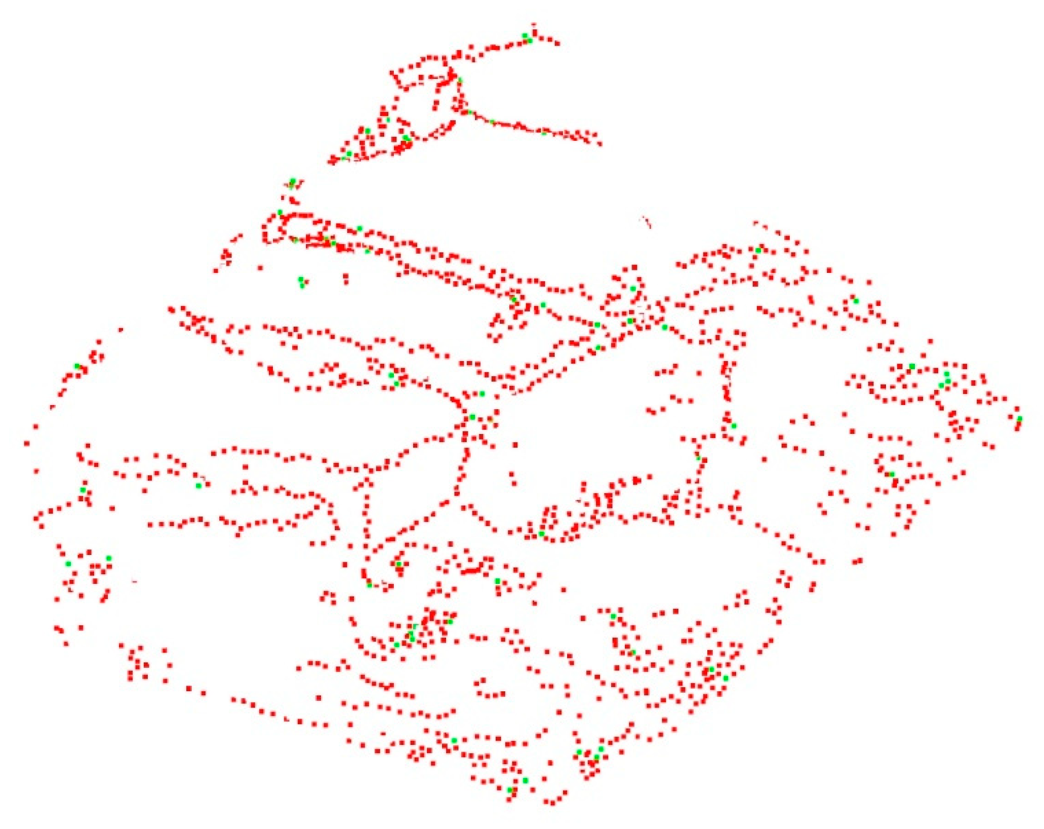
• Step 1: Detect trace feature points on the triangulated point cloud surfaces by using the normal tensor voting method;
• Step 2: Group neighboring feature points;
• Step 3: Connect feature points belonging to the same grouping to form a trace segment using a growth algorithm;
• Step 4: Connect the trace segments that may belong to one trace;
• Step 5: Calculate an estimate of the final trace length. The overall flow of the method is shown in Figure 1.

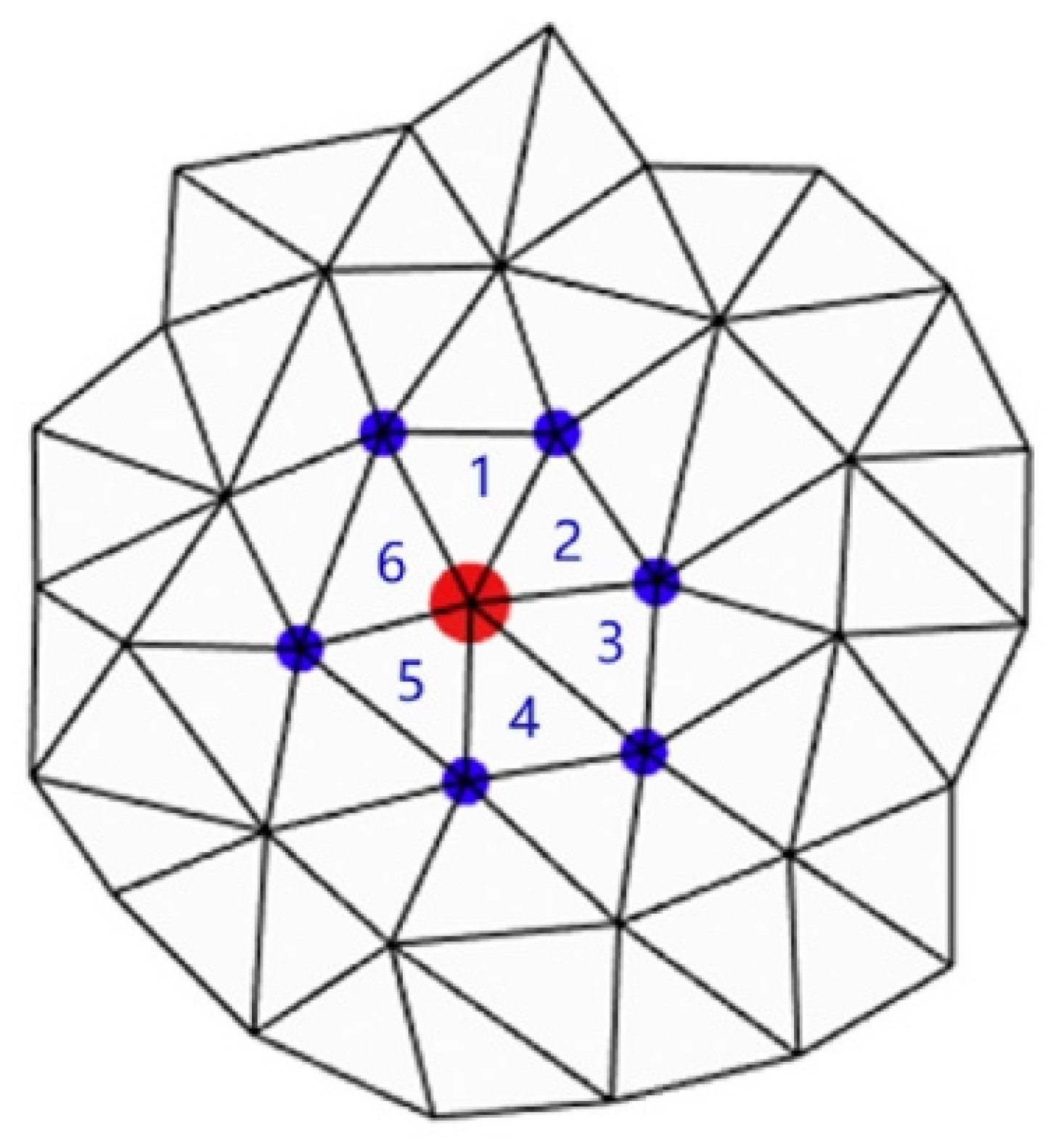
2.1. Trace Feature Point Detection by Normal Tensor Voting Method

The triangulated mesh processed from point cloud data can be used to build a skeleton of the rock mass structure by extracting the vertices at the edges or corners of the mesh, thereby identifying the traces of the rock mass. The structural surfaces of a rock mass include joint surfaces, laminated surfaces, faults, and other types of cleavage surfaces, which usually form distinct junctions on both sides. These junctions often have linear features called traces. In the point cloud data, the edge regions of these structural surfaces show obvious abrupt changes in normal vectors. Therefore, the edges of structured surfaces can be effectively detected by analyzing the changes of the surface normal in the neighboring regions, so as to extract the trace features of discontinuous surfaces [22].

The normal tensor voting (NTV) method improves the feature extraction effect of the traditional tensor voting method by combining the normal vectors of the points, which improves the accuracy and efficiency of the voting process, and shows a better robustness in the case of more noise and sparse data. The voting scheme can be simply viewed as an eigenvalue analysis of the surface normals. In the normal tensor voting method, for each point $p_i$ in the dataset, an initial tensor ${\mathit{T}}_{\mathit{i}}$ and a normal vector ${\mathit{n}}_{\mathit{i}}$ are defined where, point $p_i$ votes on point $p_j$ in its neighborhood to generate a voting tensor ${\mathit{T}}_{\mathit{i}\mathit{j}}$ with the expression as in Equation (1):

$$T_{ij}=w\left(d_{ij}\right)·w\left({\mathit{n}}_{\mathit{i}},{\mathit{n}}_{\mathit{j}}\right)·{\mathit{e}}_{\mathit{i}\mathit{j}}{\mathit{e}}_{\mathit{i}\mathit{j}}^{\mathit{T}}$$

(1)

where $w\left(d_{ij}\right)$ is the distance weight, $w\left({\mathit{n}}_{\mathit{i}},{\mathit{n}}_{\mathit{j}}\right)$ is the normal vector weight, ${\mathit{e}}_{\mathit{i}\mathit{j}}$ is the unit vector pointing from $p_i$ to $p_j$, and ${\mathit{e}}_{\mathit{i}\mathit{j}}{\mathit{e}}_{\mathit{i}\mathit{j}}^{\mathit{T}}$ is the second-order tensor used for the voting direction, which represents the feature information along ${\mathit{e}}_{\mathit{i}\mathit{j}}$.

The distance weight $w\left(d_{ij}\right)$ is usually a Gaussian function, and the weight varies with the distance from the neighboring point to the current point, and the larger the distance, the smaller the weight, as shown in Equation (2):

$$w\left(d_{ij}\right)=exp\left(-{\displaystyle \frac{d_{ij}^2}{{2\sigma }^2}}\right)$$

(2)

where $d_{ij}$ denotes the distance from point $p_j$ to point $p_i$, and σ is the scale parameter that controls the influence range of the vote.

The normal vector weights $w\left({\mathit{n}}_{\mathit{i}},{\mathit{n}}_{\mathit{j}}\right)$ are usually used as a measure of similarity using the cosine of the angle of the normal vector pinch, and the expression is shown in Equation (3):

$$w\left(n_i,n_j\right)=\cos {\theta }_{ij}={\displaystyle \frac{{\mathit{n}}_{\mathit{i}}\cdot {\mathit{n}}_{\mathit{j}}}{‖{\mathit{n}}_{\mathit{i}}‖‖{\mathit{n}}_{\mathit{j}}‖}}$$

(3)

where ${\mathit{n}}_{\mathit{i}}$ and ${\mathit{n}}_{\mathit{j}}$ are the normal vectors of the points $p_i$ and $p_j$, respectively.

The voting tensor ${\mathit{T}}_{\mathit{i}\mathit{j}}$ of all points $p_j$ in the neighborhood of point $p_i$ is accumulated to obtain the final tensor ${\mathit{T}}_{\mathit{i}}$ of point $p_i$ as shown in Equation (4):

$${\mathit{T}}_{\mathit{i}}={\sum }_{j\in S}{\mathit{T}}_{\mathit{i}\mathit{j}}$$

(4)

where S is the domain of point $p_i$.

In this paper, we perform Delaunay triangulation on a point cloud and then give an M = (P,E,T) to represent these triangle meshes. Where P = {$p_1$, $p_2$, …, $p_n$} denotes a set of vertices in the mesh, E denotes the common edges of neighboring triangles, and T = {$t_1$, $t_2$, …, $t_m$} denotes the set of triangle faces in the mesh. These triangle faces are described by the vertex indices. In this case, the expression of the normal tensor voting method needs to be adapted accordingly, and the normal vectors of each triangle in the triangular mesh structure can be used to optimize the voting process. The domain object is transformed from an original single point to a triangle containing this point, which in turn needs to replace the original vectors between points based on the normal vectors of these triangles, as shown in Equation (5):

$${\mathit{T}}_{\mathit{i}}={\sum }_{j\in S_{t\left(p\right)}}{\mu }_{ti}{\mathit{n}}_{\mathit{t}\mathit{i}}{\mathit{n}}_{\mathit{t}\mathit{i}}^{\mathit{T}}$$

(5)

where ${\mathit{n}}_{\mathit{t}\mathit{i}}$ is the normal vector of the triangle $t_i$, $S_{t\left(p\right)}$ is the unicyclic neighborhood surface index of the point $p_i$ (as in Figure 2), and ${\mu }_{ti}$ is the weighting coefficient proposed by Kim et al. [23], with the specific expression that is given below as follows:

$${\mu }_{ti}={\displaystyle \frac{A\left(t_i\right)}{A_{max}}}·exp\left(-{\displaystyle \frac{‖c_{t_i}-p‖}{\sigma /3}}\right)$$

(6)

where $A\left(t_i\right)$ is the area of triangle $t_i$, $A_{max}$ is the maximum area of $A\left(t_i\right)$, $c_{t_i}$ is the center of the mass of triangle $t_i$, and σ is the length of the side of the smallest cube containing the triangle.

In Equation (5), ${\mathit{T}}_{\mathit{i}}$ is a symmetric semipositive definite matrix and thus can be expressed as in Equation (7):

$${\mathit{T}}_{\mathit{i}}={\lambda }_1{\mathit{e}}_1{\mathit{e}}_1^{\mathit{T}}+{\lambda }_2{\mathit{e}}_2{\mathit{e}}_2^{\mathit{T}}+{\lambda }_3{\mathit{e}}_3{\mathit{e}}_3^{\mathit{T}}$$

(7)

where ${\lambda }_1$, ${\lambda }_2$, and ${\lambda }_3$ are the eigenvalues of ${\mathit{T}}_{\mathit{i}}$ and ${\lambda }_1\ge {\lambda }_2\ge {\lambda }_3\ge 0$. ${\mathit{e}}_1$, ${\mathit{e}}_2$, and ${\mathit{e}}_3$ are the unit eigenvectors corresponding to the eigenvalues.

The vertices can be classified into three different types based on different eigenvalues, which are faceted, sharp-edged, and angular [23]. The classification rules are as follows:

(1)

If ${\lambda }_1$ is dominant and when ${\lambda }_2$ and ${\lambda }_3$ can be neglected, the vertex is the face type;

(2)

If ${\lambda }_1$ and ${\lambda }_2$ are dominant and when ${\lambda }_3$ can be neglected and not remembered, the vertex is of the sharp edge type;

(3)

If ${\lambda }_1$, ${\lambda }_2$, and ${\lambda }_3$ are approximately equal, then the vertices are of the angular type.

After the above processing to divide all the point clouds into three types, the feature points referred to in this paper consist of the vertices of the above three types: face type, sharp edge type, and corner type.

In order to filter out the key feature points that can reflect the trace of the rock structure surface from many feature points, two thresholds $\alpha$ and $\beta$ are introduced in this paper to control the detection of corner-type and sharp-edge-type vertices, respectively. Firstly, the two thresholds can be initially set according to the requirements, and then the thresholds are further adjusted to optimize the results by visually and intuitively evaluating the number of detected corner-type and sharp-edge-type vertices. Specifically, the value of threshold $\alpha$ should be large enough to avoid extracting too many false corner points, while threshold $\beta$ should be carefully adjusted within a certain range to balance the relationship between the detection of weak features and the number of noise points to achieve the best results [2]. The definition of the thresholds $\alpha$ and $\beta$ depends on the visual assessment of the number of recognized edge types and corner-type vertices.

The value of threshold α controls the number of corner points. A smaller $\alpha$ will lower the screening threshold for feature points and thus will increase the number of corner points, and vice versa; with the threshold $\alpha$ determined first, the ratio of face-type points to sharp-edge-type points is controlled by the threshold $\beta$. A larger threshold $\beta$ will generate more facet points and conversely a smaller threshold $\beta$ will generate more edge points. The initial results of the facet point detection are shown in Figure 3. It is chosen to mark the corner points with green dots and the sharp-edge-type points with red dots, while the face-type points are mostly distributed at the plane and are not involved in the trace feature study and are not colored to highlight the trace features.

2.2. Grouping of Trace Feature Points

All of the feature points that make up the trace of the rock mass trace are obtained by the above analysis step. However, what is obtained by only one step of feature point extraction is the entire trace profile, and feature points representing different traces are stored in the same point set. Therefore, it is necessary to divide the overall trace profile and divide adjacent feature points with similar characteristics into the same group to obtain trace features that are locally similar to the structural surface of the rock mass. In grouping, we divide the feature points that simultaneously satisfy the following conditions at the same time into one group: (1) The feature points share the same edge of the triangulated mesh. After triangulating the mesh, the mesh where the angular and sharp-edged feature points are located must be in the vicinity of the trace, coupled with the use of triangular connections, so that the neighboring feature points share the same edge. (2) The angle of the normal vector of the feature points is less than the threshold value ${\theta }_1$. By limiting the angle of the normal vector of the feature points, it prevents the occurrence of a too-large grouping while keeping the distribution of the feature points within the same group as consistent as possible. In addition, due to the existence of corner points, the intersection points of different traces appear at the corner points, by which different traces can be separated. After testing the data, the initial value of the threshold ${\theta }_1$ can be temporarily set to 60°.

The steps for grouping are roughly as follows:

(1)

Place the angular and acute-edge points of the feature points into a separate set. One feature point is randomly selected as the initial point;

(2)

Calculate the angle between the current feature point and the normal vectors of the neighboring points, and compare it with the threshold value, and finally divide it into the same group;

(3)

Compare all the points found until there is no feature point that satisfies the threshold condition. Then, the current grouping is completed, and the next group is started;

(4)

Repeat the above steps for the remaining feature points until all the feature points are grouped.

Through the above steps, the feature points are grouped into different groups, and each group consists of neighboring feature points. The results of the rock surface characterization after grouping are shown in Figure 4. As can be seen from the groups within the rectangular area in Figure 4, the same grouping contains feature points with multiple traces, and these traces with different traces increase the difficulty of growing trace segments within a group. In addition, a trace may also be spread over several adjacent groups, so after connecting the traces of the feature points, it is also necessary to connect the traces of the adjacent subgroups to form consecutive trace segments in order to best describe a complete trace.

2.3. Grouping of Traces Growth

In the analysis of rock mass point cloud data, the simple point cloud data does not fully reflect the direction and structural characteristics of the rock mass surface traces. In order to more accurately grasp the direction of the surface traces of the rock mass, the grouped points are connected to identify the trace direction, etc.

Currently, the Principal Component Analysis (PCA) method is the most common method used to connect the traces within a grouping. However, the point cloud data of rock bodies usually have a more complex spatial structure and often exhibit irregularities and variability. Determining the main direction by PCA alone cannot connect all the branching traces. In contrast, the Minimum Spanning Tree (MST) method can not only overcome the limitations of the PCA method, but also better reflect the real structure of the rock data. This method realizes the connectivity of traces by connecting all points in the graph and minimizing the total weight. The endpoints in the above grouping can be labeled using the MST method and used as the basis for trace growth, as shown in Figure 5.

The steps for grouped trace segment growth in this paper are roughly as follows:

(1)

Process each grouping using the MST algorithm to find the possible endpoints in the group;

(2)

Select the endpoints of the group that are furthest apart, specifying the direction of the line between the two points as the direction of the subject’s connecting line;

(3)

Find the surrounding neighboring feature points using one of the subject endpoints as the starting point, which is also the current connecting point;

(4)

Calculate the angle between the connecting line between the current point and the neighboring points and the main body connecting line, give an angle threshold of θ₂, and connect the line if the angle is within the threshold;

(5)

The body’s connecting lines are connected according to the Euclidean distance, and its connecting lines will be used as the body part of the current grouping;

(6)

Since groupings containing multiple traces exist, after the subject is identified, the remaining endpoints are connected with the subject as the target until they are merged into the subject.

2.4. Trace Segments Connection

The above growth process implements the concatenation of trace feature points within a grouping, but since a single trace may be spread across multiple adjacent groups, it is also necessary to reclassify the traces of neighboring groupings. If the same attribute conditions are satisfied between adjacent groups, indicating that they come from the same trace, then two neighboring groups can be merged together to form a continuous trace segment as a way to represent a continuous trace. In this paper, we compare the angle of the main body connecting line between groups to determine whether they come from the same trace. Each end point of the body line can represent the start or end point of the group to be connected. The connecting criterion of the trace section is that the connecting line between the groups satisfies the angle threshold ${\theta }_3$ and the distance between the endpoints satisfies the threshold $d$. The overall effect of the connecting part of the trace section is shown in Figure 6, and the connected groups are indicated by the same or similar colors.

2.5. Calculation of Mean Trace Length

The mean trace length estimation methods mainly include the line estimation method, the rectangular sampling method, and the circular window sampling method. Since the circular window sampling method does not need to consider the nodal production distribution and does not need to perform integration operations when estimating the mean trace length, the circular window sampling method is used to estimate the mean trace length in this paper [24]. A trace sampling program is used for sampling [10]. The relationship between the circular window sampling window and the nodal trace is shown in Figure 7. In the round window sampling method, the traces can be classified into three different types according to the different positional relationships with the sampling window, which are penetrating, intersecting, and inwardly wrapped; penetrating is a trace with both ends outside the window, intersecting is a trace with only one end inside the window, and inwardly wrapped is a trace with both ends inside the window. Let their numbers be $L_0$, $L_1$, and $L_2$ in that order, then the total number of traces is $L=L_0+L_1+L_2$, to obtain the average trace length formula as in Equation (8):

$$s={\displaystyle \frac{\pi \left(L+L_0-L_2\right)}{2\left(L-L_0+L_2\right)}}r$$

(8)

where $r$ is the sampling radius of the circular sampling window.

The sample plane for the circular window method in the first dataset is shown in Figure 8. The traces are orthogonally projected onto the sampling plane (x-y plane). Then, the centers of nine circular windows with different radii are placed symmetrically in the sampling area. The radii were 10%, 15%, 20%, 25%, 30%, and 40% of the length of the short side of the sample region.

Despite the wide applicability of the circular window sampling method, it may lead to incomplete sampling if the window at the data boundary does not completely cover the target area. Therefore, this paper considers weighting the different types of traces in the sampling window according to the percentage of the number. Since nine circular windows with different radii are used for sampling simultaneously in this paper, the number of traces in different windows will vary. Therefore, in this paper, weights are assigned to the three types of traces to ensure that the more numerous types have larger weights for the same radius. The weights are defined as follows:

$$w_n={\sum }_{n=0}^2{\displaystyle \frac{L_n}{L}}$$

(9)

where $L$ is the total number of traces, $L_n$ is the different types of traces in the sampling window, and the values of $n$ are 0, 1, and 2. From Equations (8) and (9), the formula for the final average trace length is as shown in Equation (10):

$$s={\displaystyle \frac{\pi \left(L+w_0{L}_0-w_2{L}_2\right)}{2\left(L-w_0{L}_0+w_2{L}_2\right)}}r$$

(10)

3. Results

In this section, we conduct the experiment analysis by using two different types of rock mass point clouds. The first rock mass point cloud dataset is derived from LiDAR data available in the open repository Rockbench [18]. It originates from a natural rock mass outcrop at a roadcut slope in Ouray, Colorado, USA, as shown in Figure 9. The point cloud was acquired using an Optech Ilris3D scanner and consists of 1,040,956 points with a resolution of approximately 2 cm, as shown in Figure 9b. The second dataset consists of rock mass point cloud data collected from an exposed rock mass area, as shown in Figure 10. The study area is marked by a red box in Figure 10b and contains 501,329 points in the point cloud.

3.1. The Effect of Different Parameters

The triangular grid cell size for resampling, the angle threshold ${\theta }_2$ in the grouped trace growth step, the angle threshold ${\theta }_3$ in the intergroup trace joining step, and the distance threshold d are all important parameters of the semi-automatic trace mapping method. This chapter focuses on the effect of these parameters on the final average trace length estimation.

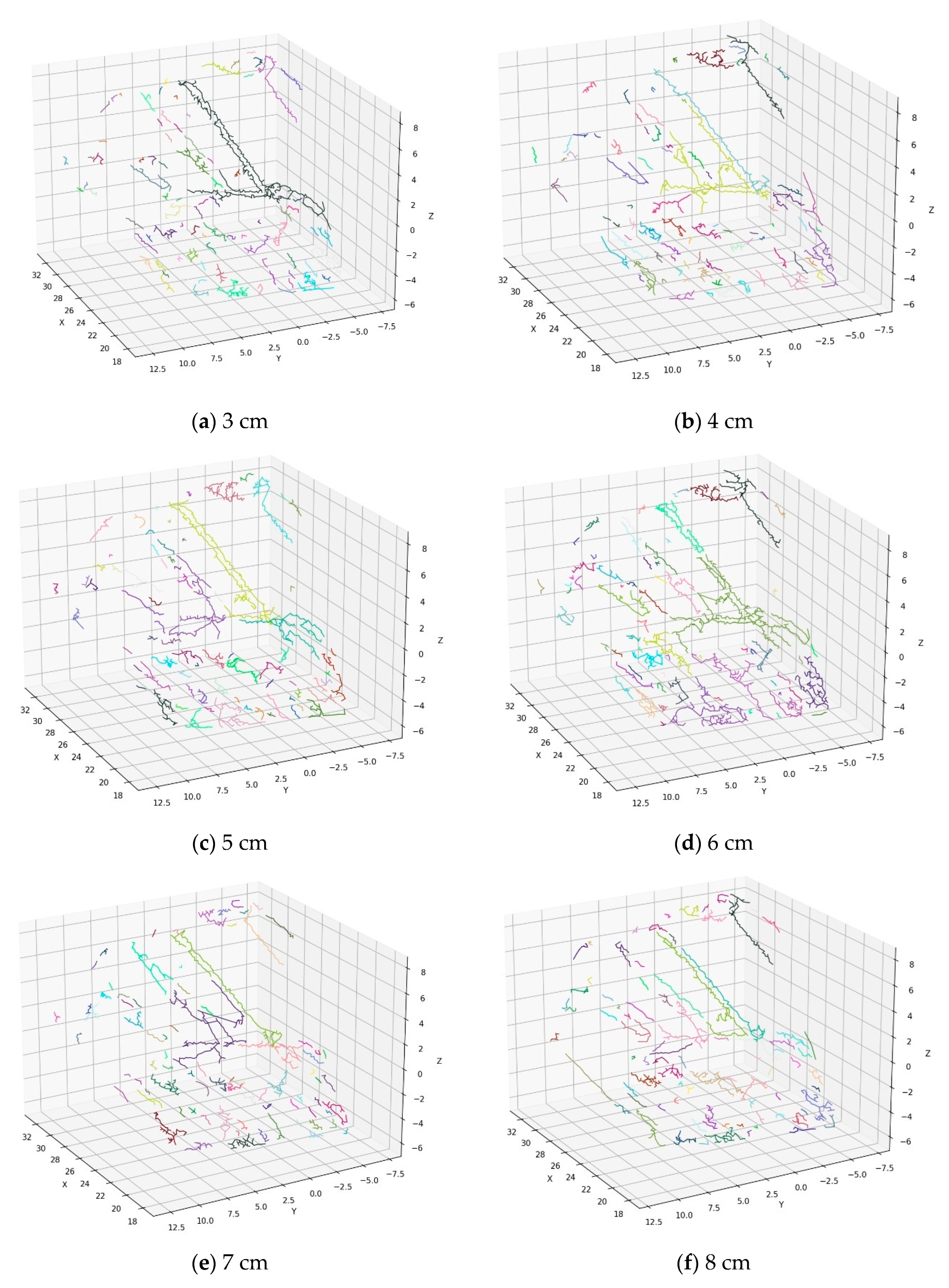
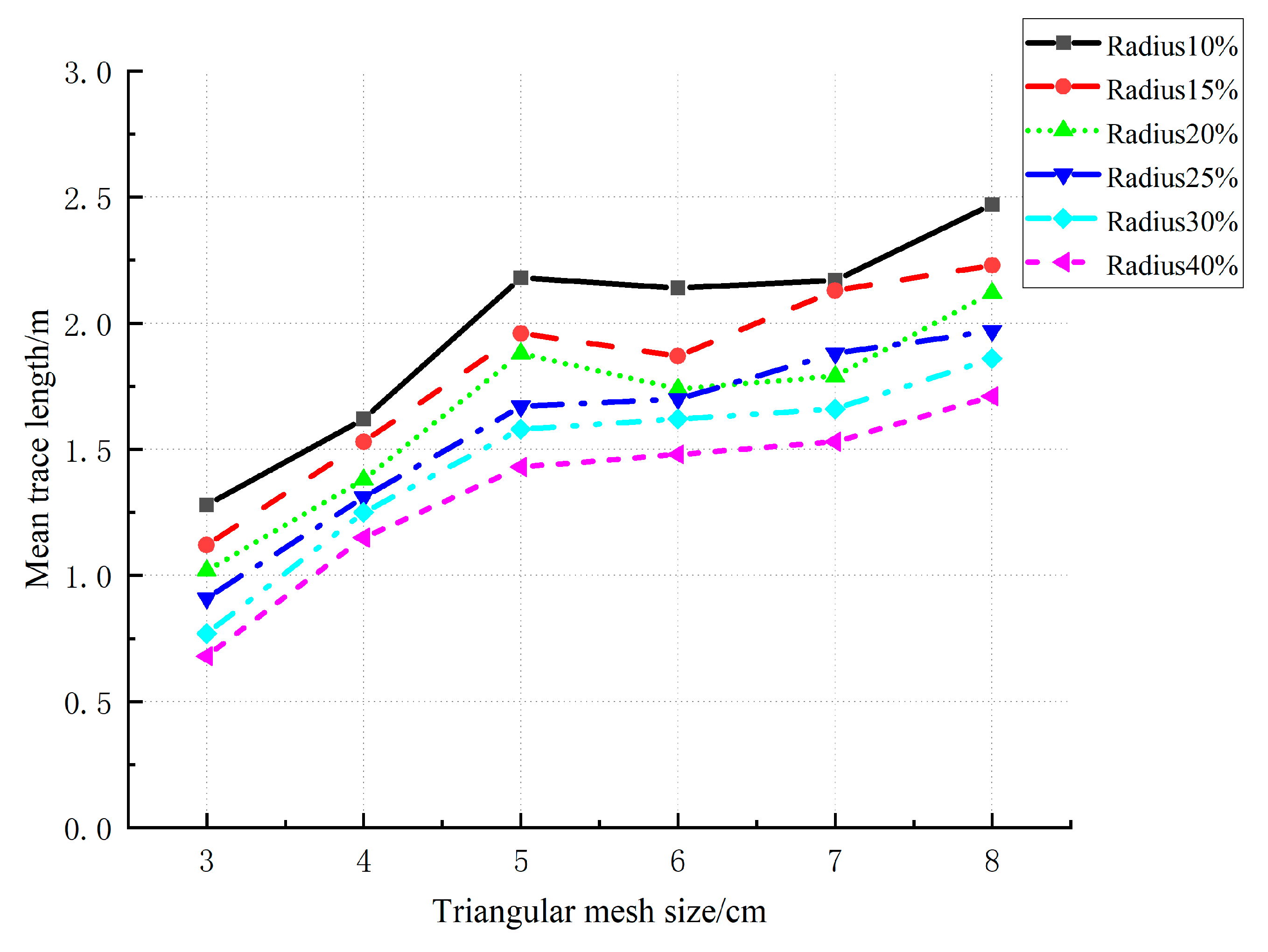
3.1.1. The Effect of Resampled Triangular Grid Cell Sizes

The effect of the resampling size on point cloud data is multifaceted. A smaller resampling size helps to preserve details and improve accuracy, thus better capturing the finer geometric features and complex details of objects in space, but increases the computational burden and data storage requirements, while a larger resampling size improves computational efficiency but may lead to the loss of some details.

In this paper, different triangle mesh sizes of 3 cm, 4 cm, 5 cm, 6 cm, 7 cm, and 8 cm are used to resample the original point cloud. The trace results are obtained by the above steps and are shown in Figure 11. It can be clearly seen from Figure 11 that the number of fine discontinuous traces decreases as the resampling triangle mesh size increases.

The relationship between the changes in the relative mean trace lengths for different sampling radii for different triangular grid sizes is shown in Figure 12. As can be seen from Figure 12, as the triangular grid size increases, the average trace length first shows an upward trend, then tends to stabilize, and then continues to show an upward trend. In addition, when the triangular grid cell size is small, many fine, discontinuous traces are generated on the rock surface. Some of these fine traces reflect small nodal variations on the rock mass surface, and others are due to significant changes in nodal orientation in the discontinuous regions that prevent the traces from connecting. However, the surface of the triangulated model becomes progressively smoother as the triangular grid cell size increases. As a result, the uneven ridges as well as the nodal surfaces are gradually reduced, and some of these fine traces are integrated into the model surface due to the change in processing accuracy, while others are connected to the continuous traces. As a result, when the triangular grid cell size is between 3 cm and 5 cm, the average trace length obtained increases as the grid size increases. When the triangular grid cell size is between 5 cm and 7 cm, the average trace length tends to stabilize because the fine traces and the fine trace connections are no longer detected. However, when the triangular grid size exceeds 7 cm, erroneous connections occur between some of the traces, causing the resulting average trace length to also become too large, and this phenomenon of trace length growth due to erroneous connections tends to result in an erroneous trace length estimation. Therefore, the optimal triangular grid cell size was determined to be between 5 cm and 7 cm.

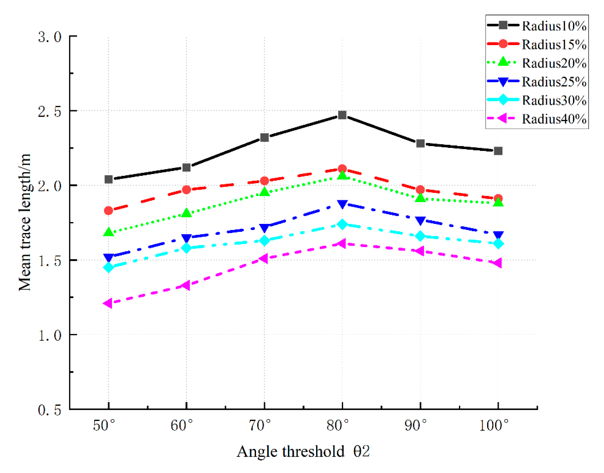
3.1.2. The Effect of the Angular Threshold ${\theta }_2$

According to Section 3.1.1, the triangular grid cell size is kept as 5 cm. The angle threshold ${\theta }_2$ is taken as six values of 50°, 60°, 70°, 80°, 90° and 100°. The variation of the obtained mean trace length with respect to the angle threshold ${\theta }_2$ is shown in Figure 13. According to the results shown in Figure 13, the average trace length gradually increases and then slightly decreases with the increase of the threshold value ${\theta }_2$. The reason for this result is that the triangular mesh tends to be distorted in irregular and uneven regions such as discontinuous surfaces, so the growth of trace segments is easily interrupted at the distorted locations when the value of the threshold ${\theta }_2$ is small, and when the value of the threshold ${\theta }_2$ is too large, trace segments deviating from the straight line are generated and cannot be connected in the subsequent step of connecting between the groups of traces. Another part of the reason is that when the threshold ${\theta }_2$ is taken at a small value, the connecting line will select a point that is farther away from the connecting line, resulting in the generation of fewer trace segments during the growth process, and the number of traces obtained during the sampling process will be reduced; on the contrary, if the threshold value ${\theta }_2$ is set at too large a value, although the distortion of a part of the irregular region is alleviated, due to the threshold value being too high, part of the simpler and regular region may be be ignored and part of the complex regions, the growth process of the linking algorithm, may appear jagged, resulting in an increase in the number of traces obtained during the sampling process. In addition, a threshold that is too high may also result in the loss of detail, especially in some boundary or transition regions, which will affect the accuracy of the results. When ${\theta }_2$ takes a value between 70°and 90°, the average trace length is relatively large. Therefore, the optimal angle of the threshold ${\theta }_2$ in the grouped trace growth step may be set between 70°and 90°.

3.1.3. The Effect of the Distance Threshold d

In this section, the triangular grid cell size is fixed to 5 cm, the angle threshold ${\theta }_2$ is 80°, and the angle threshold ${\theta }_3$ is 60°. The distance threshold d takes five values of 5 L, 10 L, 15 L, 20 L, and 25 L, where L is the triangular grid cell size. The variation of the obtained mean trace length with respect to the distance threshold $d$ for different sampling radii is shown in Figure 14. From Figure 14, it can be clearly seen that the average trace length continuously increases with the value of the distance threshold $d$ until it reaches a stable level. The reason is that when the distance threshold $d$ is small, there are only fewer or no other groups existing within the distance range, and even no inter-group trace segments are generated between the groups, and the average trace length responds less to the change of the threshold $d$, making the average trace length smaller. As the distance threshold d increases, the number of groups within the distance d also increases, the number of traces obtained in the sampling process increases, and the calculated average trace length gradually increases. In addition, when the value of the distance threshold $d$ is increased to a certain extent, the number of effective traces obtained in the sampling process tends to stabilize, and therefore the trace length also tends to stabilize. When the value of the distance threshold $d$ is taken near 15 L, the average trace length gradually tends to stabilize. Therefore, the optimal distance threshold $d$ in the connectivity algorithm should be set to be at least 15 times the average triangular grid cell size.

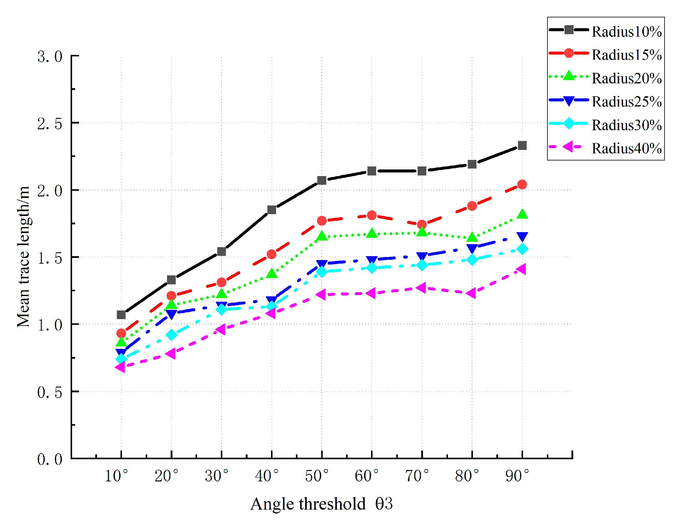
3.1.4. The Effect of the Angular Threshold ${\theta }_3$

The angle threshold ${\theta }_3$ takes nine values of 10°, 20°, 30°, 40°, 50°, 60°, 70°, 80°, and 90°, at which time the triangular grid cell size is fixed at 5 cm, the angle threshold ${\theta }_2$ is 80°, and the distance threshold $d$ is taken to be 15 times the size of the triangular grid cell at the optimal distance. Figure 15 shows the relationship between the change of the average trace length relative to the angular threshold ${\theta }_3$ for different sampling radii. From Figure 15, it can be clearly seen that the average trace length first increases gradually and then decreases slightly as the threshold value ${\theta }_3$ increases. When the value of the angle threshold ${\theta }_3$ is increased from 10° to 40°, the average trace length gradually increases and then stabilizes between 50° and 70°, but after 70°, the average trace length appears to continue to increase. The reason is that when the value of the angular threshold ${\theta }_3$ is taken between 10° and 40°, as the threshold ${\theta }_3$ increases, the groups that are in the surrounding area gradually comply with the distance condition, the line segments near the direction of the connecting lines of the main bodies of the groups are continuously connected, and most of the groups that are in the same trace are in the threshold interval, which leads to the gradual increase of the average trace length. When the angular threshold ${\theta }_3$ is between 50° and 70°, most of the groups in the same trace have been connected to each other, and the average trace length tends to stabilize at this time. However, when the value of the angle threshold ${\theta }_3$ is taken to be greater than 70°, there may be a situation in which the line segments are incorrectly connected, and some groups that do not belong to the same trace may be incorrectly connected, causing the average trace length to increase again. Therefore, the optimal angle of the threshold ${\theta }_3$ in the step of connecting the traces between groups may be set between 50° and 70°.

3.2. Comparative Analysis

The results of the method in this paper are compared with the results of the conventional growth method, as shown in Figure 16. Figure 16a shows the results of conventional growth, while Figure 16b shows the results of the proposed method. The comparison in Figure 16a,b demonstrates a comparable extraction efficacy between the conventional growth-based approach and our proposed methodology in extracting rock mass point cloud trajectories. However, the methodological comparison reveals a critical performance discrepancy: as highlighted in the red rectangular boxes in Figure 16a,b, our approach successfully identified four additional rock mass discontinuity traces compared to the conventional growing technique, quantitatively demonstrating its enhanced detection capability. Meanwhile, the traditional growth method retains some redundant rock mass traces, as shown in the oval frame in Figure 16a, while the method in this paper successfully removes these redundant rock mass traces, as shown in the oval frame in Figure 16b. In addition, the trace connection effect in the discontinuous surface region of the method of this paper is significantly improved compared with the conventional method, as shown in the black rectangular box.

The results of the method of this paper are compared with those of Zhang et al. [25], as shown in Figure 17. Figure 17a shows the results of the method of Zhang et al., while Figure 17b shows the results of the method of this paper. As demarcated by the red rectangular annotations in Figure 17a,b, it is revealed that our methodology detects three additional rock mass discontinuities compared to the growing algorithm proposed by Zhang et al. Moreover, the proposed method demonstrates a superior rock trace connectivity preservation in discontinuous surface regions when benchmarked against Zhang et al.’s approach, as evidenced by the enhanced rock trace continuity within the black rectangular annotation in Figure 17a.

3.3. Noise Resistance Analysis

To verify the effectiveness and stability of the feature point and trace extraction method in this paper, Gaussian noise of 0.005 m, 0.05 m, 0.01 m, and 0.1 m is added to the original point cloud data, respectively. With different degrees of Gaussian noise, the extracted feature points are shown in Figure 18. Figure 18a–d show the detected feature points after adding 0.005 m, 0.05 m, 0.01 m, and 0.1 m Gaussian noise in order. From the figure, it can be seen that as the noise increases, a small number of noise points are detected as redundant points, causing the number of feature points to increase slightly, but the overall contour of the structural surface of the rock mass can still be successfully obtained.

As can be clearly seen from Figure 19, the trace extraction results under different noise levels also show slight variations. It can be clearly seen from Figure 19 that the trace extraction effect is slightly different under different noise levels. Under a Gaussian noise level of 0.005 m, the proposed method successfully extracted almost all fracture traces in the rock mass, with numerous long fracture traces exhibiting no apparent discontinuities, as demonstrated in Figure 19a. When the Gaussian noise increases to 0.01 m, almost all the long rock mass trace lines are successfully extracted by the proposed method. However, some of the long rock mass trace lines exhibit breaks, as shown in the rectangular box in the upper right corner of Figure 19b. When the Gaussian noise is 0.005 m, the rock mass trace lines in the same region are continuous, as shown in the rectangular box in the upper right corner of Figure 19a. When the Gaussian noise increases to 0.05 m, the proposed method still successfully extracts the rock mass trace at this noise level, and the extraction results are similar to those in Figure 19a,b. Similarly, a small number of long traces appear discontinuous, as shown in the top right rectangular box of Figure 19c. When the Gaussian noise increases to 0.1 m, many of the rock mass traces become discontinuous, and some of the shorter traces cannot be extracted, as shown in the rectangular box in Figure 19d. However, as can be seen from Figure 19d, the overall rock mass trace lines are not significantly different from those at other noise levels. As can be seen from the above analysis, as the noise increases, it has little effect on the overall trace extraction, although it contains a small number of redundant points. Therefore, from the results in Figure 19, it can be concluded that the method in this paper is robust.

3.4. Case Study

For the second dataset used in this paper, the trace extraction is performed using the discontinuous trace mapping method steps proposed in this paper, and the average trace length estimation is performed using the circular window sampling method. During the processing of each step, the range of each threshold value is adopted from the above analysis as a way to verify whether the data is reliable.

In the feature point detection step, the initial feature vertices are extracted using the normal tensor voting method, as shown in Figure 20a. Then, the grouping of feature points, the extraction of the end points of each group, and the connection of the traces between the groups are carried out using steps I to IV of the method in this paper, respectively, as shown in Figure 20c,d. As can be seen from Figure 20a, the proposed method successfully extracted almost all trace feature points of the rock mass structural plane. Moreover, the extracted feature points do not contain many redundant points. As can be seen from the feature points of different colors in Figure 20b, the feature points of each trace are grouped separately by the method presented in this paper. However, it can be seen from the feature points in the adjacent grouping that some feature points that should belong to one trace are grouped into two. The reason for this grouping is that there are some redundant points or discontinuities directly in the feature points adjacent to the grouping. In order to obtain the grouping of the same feature points more precisely and avoid the wrong grouping of feature points, it is divided into two adjacent groups. The two endpoints of each trace, as shown in Figure 20c, can then be connected to form a grouping trace. It can be clearly seen from Figure 20d that the trace formed after the intergroup trace segments are connected by this method, making the discontinuous traces more continuous and shows the characteristic line of the rock mass structural plane more clearly. The resulting traces are orthogonally projected onto the sampling plane in an orthogonal manner. The average trace length was calculated using the centers of nine circular windows with seven different radii placed symmetrically on the sampling area for sampling, and the sampling area effect is shown in Figure 21. The final calculation of the ground-averaged trace length calculation for the different sampling radii is shown in

Table 1. The mean trace lengths at different sampling radii.

Sampling Radii/m	Mesh Size/cm	Angle Threshold θ2	Angle Threshold θ3	Distance Threshold d	Mean Trace Lengths/m
10%	5	80°	60°	$15L$	0.83
15%	5	80°	60°	$15L$	0.97
20%	5	80°	60°	$15L$	1.34
25%	5	80°	60°	$15L$	1.18
30%	5	80°	60°	$15L$	1.04
35%	5	80°	60°	$15L$	0.92
40%	5	80°	60°	$15L$	0.85

. As shown in Figure 22, the average trace length decreases with the increase of the sampling radius value and gradually reaches a stable level. According to Table 1, the average trace length of the rock mass structural plane is obtained, which is used as an important parameter for describing the extent and distribution scale of structural surfaces, and it plays a significant role in the stability analysis of rock masses.

3.5. Discussion

The extraction of structural discontinuity traces and their length quantification in rock masses hold significant implications for both theoretical research and engineering applications. As primary geometric descriptors of fracture networks, these traces serve as fundamental parameters for analyzing rock mass mechanical behavior, including but not limited to strength anisotropy, permeability characteristics, and failure mechanisms.

From an engineering geology perspective, accurate trace mapping enables the following:

(1)

A reliability assessment of the discontinuities’ spatial persistence in stability analysis.

(2)

The statistical determination of representative elementary volumes (REVs) for numerical modeling.

(3)

An objective evaluation of rock mass quality indices (e.g., RQD and GSI).

Moreover, trace-length distributions provide critical insights into geological evolution processes, allowing for a quantitative characterization of fracture propagation patterns and tectonic stress field reconstruction. The methodological advancement in high-fidelity trace extraction under noisy conditions (e.g., 0.005 m Gaussian noise) particularly enhances the feasibility of non-destructive characterization in complex field environments, bridging the gap between laboratory-scale measurements and practical geotechnical investigations.

In this paper, trace extraction and the length measurements of rock mass structural planes are realized through four steps, and the influence of different parameters on trace extraction is analyzed. According to the analysis in Figure 9, the larger the triangular mesh size, the more difficult it is to extract small discontinuous traces. Therefore, for the rock mass point cloud with a high precision and relatively simple structure, a larger triangular mesh can be selected. On the contrary, a smaller triangular mesh should be selected. According to the analysis in Figure 13, for most of the rock mass point clouds, threshold ${\theta }_2$ in the grouped trace growth step is generally set between 70° and 90°. Of course, threshold ${\theta }_2$ can be appropriately lower than 70° or higher than 90°. In the same way, the initial best values of the distance threshold $d$ and angle threshold ${\theta }_3$ are obtained from Figure 14 and Figure 15. Although the universal applicability of these determined optimal threshold parameters across diverse rock mass point clouds remains unverified, they can serve as empirical initial reference values for structural discontinuity trace extraction. Subsequent parameter tuning within constrained ranges adjacent to these baseline values enables the progressive refinement of trace identification accuracy, thus achieving optimized extraction outcomes through iterative empirical optimization. To ensure that the method proposed in this paper is applicable to large-scale rock engineering datasets, the algorithm complexity of the proposed method is designed to be low, given the large volume of point cloud data associated with rock mass structural surfaces. The proposed method mainly includes detection, grouping, and growth of trace feature points. The computational cost of these processes is low. We use python as the experimental platform, and the proposed method is applied on a computer with a hardware configuration of Intel Core i7-5500U CPU with a 2.40 GHz 4.00-GB memory and Windows 10 operating system. The experimental results demonstrate that the presented approach successfully extracted fracture traces from a rock mass point cloud dataset comprising 1,040,956 individual points, requiring less than 5 min total of a processing time. Of course, the computational efficiency of the algorithm is inherently influenced by programming paradigms, and the optimized programming strategies can reduce time complexity. Therefore, the proposed method is suitable for extracting point cloud traces of rock masses in large-scale scenarios.

The comparison between the proposed method and other methods shows that the proposed method has two main advantages, as follows:

(1)

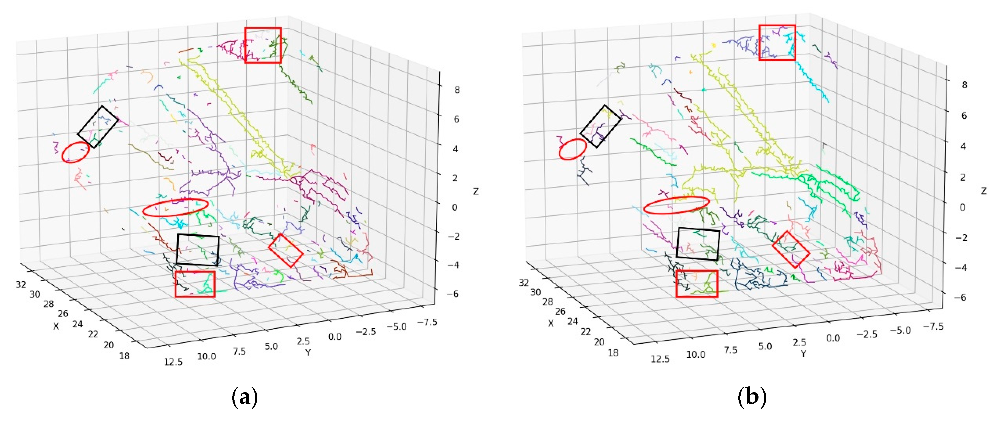
The linear extension of the detected traces is obvious, robust to noise points, and better matches the main trend of the real traces;

(2)

The proposed method is more stable, and is able to overcome the segmentation problem of trace extraction and obtain linear and continuous traces.

However, there are still shortcomings in this paper, such as the failure to summarize the optimal parameter threshold applicable to all rock mass point clouds. The method in this paper still belongs to semi-automatic rock mass trace extraction. At the same time, it can be seen from the case study of Figure 20d that there are still many discontinuities in the rock mass trace obtained by this method. Therefore, these shortcomings of the proposed method will be studied in the future, so as to achieve an automatic and high-precision rock mass trace extraction.

4. Conclusions

This paper proposes a new method of trace mapping based on the 3D point cloud of the rock surface to automatically draw the trace of the discontinuous surface. The optimal values of the different parameters of the method are determined by a sensitivity analysis of the main parameters of the method. The experimental results show that, as follows: the optimal triangular grid cell size is between 5 cm and 7 cm, the optimal range of the angle threshold θ₂ is between 70° and 90° for the grouped trace growth step, the optimal range of the angle threshold θ₃ is between 50° and 60° for the intergroup trace joining step, and the distance threshold should be taken as at least 15 times of the triangular grid cell size. The method proposed in this paper detects a greater number of rock mass trace lines compared to traditional growth methods, and the trace line connection effect on discontinuous surface areas obtained by this method is superior to that of the method of Zhang et al. In addition, the method proposed in this paper is still capable of extracting feature points and traces even after the addition of Gaussian noise, indicating that the method possesses a certain level of robustness.

The case study of this paper shows that the method can measure the geometric features of discontinuous surfaces quickly and effectively. The method can be used as a supplement to the traditional direct crack and scanning line measurements, providing an efficient detection tool for rock engineering investigation and the analysis of rock engineering. However, a disadvantage of the proposed method is that it does not provide fixed parameters applicable to all types of rock mass point clouds, thereby preventing it from achieving automated rock mass trace extraction. Moreover, the proposed method calculates the rock mass trace length based on different sampling window radii, which prevents it from obtaining the final precise trace length. Therefore, in the future, we will investigate the relationship between parameters and point cloud accuracy and density to develop a parameter model applicable to all types of rock mass point clouds. Additionally, we will explore more accurate methods for calculating rock mass trace length.

References

1. Hu, Q.; Ma, C.; Bai, Y.; He, L.; Tan, J.; Cai, Q.; Zeng, J. A Rapid Method of the Rock Mass Surface Reconstruction for Surface Deformation Detection at Close Range. Sensors 2020, 20, 5371. [Google Scholar] [CrossRef] [PubMed]
2. Mehrishal, S.; Kim, J.; Song, J.J.; Sainoki, A. A semi-automatic approach for joint orientation recognition using 3D trace network analysis. Eng. Geol. 2024, 332, 107462. [Google Scholar] [CrossRef]
3. Lemy, F.; Hadjigeorgiou, J. Discontinuity Trace Map Construction Using Photographs of Rock Exposures. Int. J. Rock Mech. Min. Sci. 2003, 40, 903–917. [Google Scholar] [CrossRef]
4. Ferrero, A.M.; Forlani, G.; Roncella, R.; Voyat, H. Advanced Geostructural Survey Methods Applied to Rock Mass Characterization. Rock Mech. Rock Eng. 2009, 42, 631–665. [Google Scholar] [CrossRef]
5. Li, X.; Chen, J.; Zhu, H. A New Method for Automated Discontinuity Trace Mapping on Rock Mass 3d Surface Model. Comput. Geosci. 2016, 89, 118–131. [Google Scholar] [CrossRef]
6. Cao, T.; Xiao, A.; Wu, L.; Mao, L. Automatic Fracture Detection Based on Terrestrial Laser Scanning Data: A New Method and Case Study. Comput. Geosci. 2017, 106, 209–216. [Google Scholar] [CrossRef]
7. Pan, D.; Li, Y.; Wang, X.; Xu, Z. Intelligent Image-Based Identification and 3-D Reconstruction of Rock Fractures: Implementation and Application. Tunn. Undergr. Space Technol. 2024, 145, 105582. [Google Scholar] [CrossRef]
8. Gigli, G.; Casagli, N. Semi-Automatic Extraction of Rock Mass Structural Data from High Resolution Lidar Point Clouds. Int. J. Rock Mech. Min. Sci. 2011, 48, 187–198. [Google Scholar] [CrossRef]
9. Lu, F.; Fu, C.; Shi, J.; Zhang, G. Attention Based Deep Neural Network for Micro-Fracture Extraction of Sequential Coal Rock Ct Images. Multimed. Tools Appl. 2022, 81, 26463–26482. [Google Scholar] [CrossRef]
10. Umili, G.; Ferrero, A.; Einstein, H. A New Method for Automatic Discontinuity Traces Sampling on Rock Mass 3d Model. Comput. Geosci. 2013, 51, 182–192. [Google Scholar] [CrossRef]
11. Vöge, M.; Lato, M.J.; Diederichs, M.S. Automated Rockmass Discontinuity Mapping from 3-Dimensional Surface Data. Eng. Geol. 2013, 164, 155–162. [Google Scholar] [CrossRef]
12. Taghizadeh, M.; Kakaee, R.K.; Nasirabad, H.M.; Alenizi, F.A. Automatic Detection of Discontinuity Trace Maps: A Study of Image Processing Techniques in Building Stone Mines. Geomech. Eng. 2024, 36, 205. [Google Scholar]
13. Chudasama, B.; Ovaskainen, N.; Tamminen, J.; Nordbäck, N.; Engström, J.; Aaltonen, I. Automated Mapping of Bedrock-Fracture Traces from Uav-Acquired Images Using U-Net Convolutional Neural Networks. Comput. Geosci. 2024, 182, 105463. [Google Scholar] [CrossRef]
14. He, Y.; Hu, Z.; Wang, R.; Zhu, H.; Fu, G. Features Extraction of Point Clouds Based on Otsu’s Algorithm. Meas. Sci. Technol. 2024, 35, 065205. [Google Scholar] [CrossRef]
15. Guo, J.; Wu, L.; Zhang, M.; Liu, S.; Sun, X. Towards Automatic Discontinuity Trace Extraction from Rock Mass Point Cloud without Triangulation. Int. J. Rock Mech. Min. Sci. 2018, 112, 226–237. [Google Scholar] [CrossRef]
16. Guo, J.; Zhang, Z.; Mao, Y.; Liu, S.; Zhu, W.; Yang, T. Automatic Extraction of Discontinuity Traces from 3d Rock Mass Point Clouds Considering the Influence of Light Shadows and Color Change. Remote Sens. 2022, 14, 5314. [Google Scholar] [CrossRef]
17. Gézero, L.; Antunes, C. Automated Road Curb Break Lines Extraction from Mobile Lidar Point Clouds. ISPRS Int. J. Geo-Inf. 2019, 8, 476. [Google Scholar] [CrossRef]
18. Ge, Y.; Cao, B.; Tang, H. Rock Discontinuities Identification from 3d Point Clouds Using Artificial Neural Network. Rock Mech. Rock Eng. 2022, 55, 1705–1720. [Google Scholar] [CrossRef]
19. Mehrishal, S.; Kim, J.; Shao, Y.; Song, J.J. Artificial intelligence-aided semi-automatic joint trace detection from textured three-dimensional models of rock mass. J. Rock Mech. Geotech. Eng. 2024; in press. [Google Scholar] [CrossRef]
20. Alseid, B.; Chen, J.; Huang, H.; Seo, H. Automatic Detection of Traces in 3d Point Clouds of Rock Tunnel Faces Using a Novel Roughness: Canupo Method. J. Civ. Struct. Health Monit. 2024, 17, 1703–1718. [Google Scholar] [CrossRef]
21. Page, D.L.; Sun, Y.; Koschan, A.F.; Paik, J.; Abidi, M.A. Normal Vector Voting: Crease Detection and Curvature Estimation on Large, Noisy Meshes. Graph. Models 2002, 64, 199–229. [Google Scholar] [CrossRef]
22. Phan, T.D.K. A Triangle Mesh-Based Corner Detection Algorithm for Catadioptric Images. Imaging Sci. J. 2018, 66, 220–230. [Google Scholar] [CrossRef]
23. Kim, H.S.; Choi, H.K.; Lee, K.H. Feature Detection of Triangular Meshes Based on Tensor Voting Theory. Comput. Aided Des. 2009, 41, 47–58. [Google Scholar] [CrossRef]
24. Zhang, L.; Einstein, H. Estimating the Mean Trace Length of Rock Discontinuities. Rock Mech. Rock Eng. 1998, 31, 217–235. [Google Scholar] [CrossRef]
25. Zhang, K.; Wu, W.; Zhu, H.; Zhang, L.; Li, X.; Zhang, H. A Modified Method of Discontinuity Trace Mapping Using Three-Dimensional Point Clouds of Rock Mass Surfaces. J. Rock Mech. Geotech. Eng. 2020, 12, 571–586. [Google Scholar] [CrossRef]
Figure 1. Flowchart of the discontinuous trace mapping method.
Symmetry 17 00415 g001
Figure 2. An example of a one-loop neighbor point and S t ( p ) . The red point denotes the point p i , the blue points around it are its one-ring neighbor points, and the blue numbers are the one-ring neighbor surface indices corresponding to the point p i ; thus, S t ( p ) = {1,2,3,4,5,6}.
Symmetry 17 00415 g002
Figure 3. The initial feature points detected using the normal tensor method. Red is sharp-edge-type points and green is corner-type points.
Symmetry 17 00415 g003
Figure 4. Feature point grouping results. Each color in (a) represents a group, and (b) is the part of the red box in (a) where the points of multiple traces are grouped in the same point set.
Symmetry 17 00415 g004
Figure 5. Groups of endpoints extracted using the MST algorithm. Endpoints are marked in red.
Symmetry 17 00415 g005
Figure 6. Traces after trace segment connection.
Symmetry 17 00415 g006
Figure 7. Schematic diagram of the circular window sampling method.
Symmetry 17 00415 g007
Figure 8. An example of the sampling for nine different positional windows.
Symmetry 17 00415 g008
Figure 9. The first rock mass point cloud dataset, (a) the rock mass image, and (b) the rock mass point cloud.
Symmetry 17 00415 g009
Figure 10. The second rock mass point cloud dataset, (a) an exposed rock mass area, and (b) the rock mass point cloud of the study area.
Symmetry 17 00415 g010
Figure 11. Trace results obtained by mapping with different triangular mesh sizes.
Symmetry 17 00415 g011
Figure 12. The average trace length for different triangular grid sizes.
Symmetry 17 00415 g012
Figure 13. The mean trace length for different angle threshold θ 2 .
Symmetry 17 00415 g013
Figure 14. The mean trace length for different distance threshold d .
Symmetry 17 00415 g014
Figure 15. The mean trace length for different angle threshold θ 3 .
Symmetry 17 00415 g015
Figure 16. Results of the traditional growth method (a) and the results of our method (b).
Symmetry 17 00415 g016
Figure 17. Results of the method of Zhang et al, 2020. (a) and the results of our method (b).
Symmetry 17 00415 g017
Figure 18. Images (ad) show the feature points after adding different sizes of Gaussian noise in turn.
Symmetry 17 00415 g018
Figure 19. Images (ad) show the traces after adding different sizes of Gaussian noise in turn.
Symmetry 17 00415 g019
Figure 20. Images (ad) show the results obtained in steps I to IV: (a) detected feature points, (b) feature point grouping, (c) the endpoints of each group, and (d) the trace after the intergroup trace is connected.
Symmetry 17 00415 g020
Figure 21. Sampling using a window of seven radii at nine different locations.
Symmetry 17 00415 g021
Figure 22. The mean trace length for different sampling window radii.
Symmetry 17 00415 g022