

Riemannian Topological Analysis of Neuronal Activity


Abstract
1. Introduction
2. Preliminary
- The values of determine the connection on the open set .
- Conversely, given a coordinate neighborhood and an arbitrary set of differentiable functions on , there exists a unique affine connection on whose Christoffel symbols in the coordinates are .
- Let be the Christoffel symbols of a connection on for the coordinate neighborhood . It follows that is symmetric on (see Definition 1) if and only if for all .
- Let be a connection on , and let and be two coordinate systems on the same open set . The relationship between the Christoffel symbols and , which are associated with their respective coordinate systems, is
- 1.
- The covariant derivative is -linear, that is,
- 2.
- The Leibniz rule for the product holds, that is,
- The parallel transport mapis a vector space isomorphism.
- If is a basis of and are the corresponding vector fields along obtained by the parallel transport of the vectors , respectively, then any parallel vector field along can be written as
- The following equality holds: ,
- It is possible to reconstruct the connection from the parallel transport. Indeed, for each vector field and each curve in , the vector field can be expressed in terms of the parallel transport map, which is as follows:
- (i)
- (;
- (ii)
- is inextensible (or maximal), that is, there does not exist another geodesic that satisfies (i) and whose domain of definition strictly contains .
3. Results
- (a)
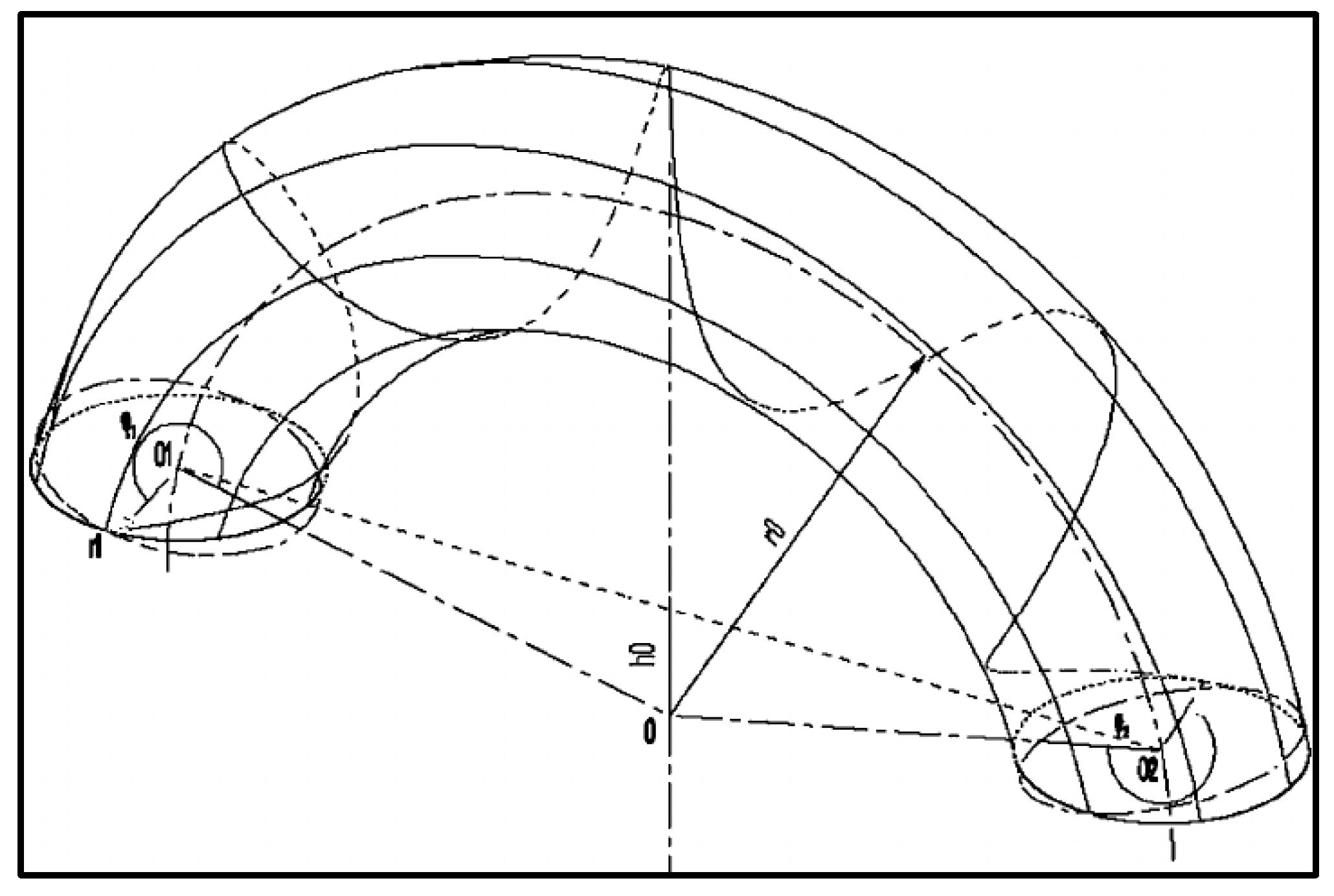
- and have values such that , and the geodesics wind around the torus.
- (b)
- and have values such that , and then the geodesic is asymptotic to the circle
- (c)
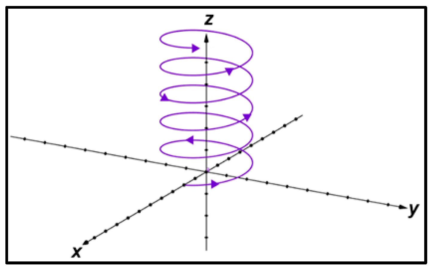
- and have values such that , and then the only geodesics in this case are the curves that wind around the torus in the manner of circular helices on a cylinder (see Figure 2), the meridians, and the parallels.
4. Discussion
5. Conclusions
Author Contributions
Funding
Data Availability Statement
Conflicts of Interest
References
- Curto, C. What can topology tell us about the neural code? Bull. Amer. Math. Soc. 2017, 54, 63–78. [Google Scholar] [CrossRef]
- Bruner, E.; Esteve-Altava, B.; Rasskin-Gutman, D. A network approach to brain form, cortical topology and human evolution. Brain Struct. Funct. 2019, 224, 2231–2245. [Google Scholar] [CrossRef] [PubMed]
- Gastner, M.T.; Odor, G. The topology of large Open Connectome networks for the human brain. Sci. Rep. 2016, 6, 27249. [Google Scholar] [CrossRef]
- Yang, Y.M.; Chang, K.C.; Luo, J.N. Hybrid neural-based intrusion detection system: Leveraging LightGBM and MobileNetV2 for IoT security. Symmetry 2025, 17, 314–333. [Google Scholar] [CrossRef]
- Gardner, R.J.; Hermansen, E.; Pachitariu, M.; Burak, Y.; Baas, N.A.; Dunn, B.A.; Moser, M.-B.; Moser, E.I. Toroidal topology of population activity in grid cells. Nature 2022, 602, 123–128. [Google Scholar] [CrossRef]
- Kang, L.; Xu, B.; Morozov, D. Evaluating state space discovery by persistent cohomology in the spatial representation system. Front. Comput. Neurosci. 2021, 15, 616748. [Google Scholar] [CrossRef]
- De Silva, V.; Morozov, D.; Vejdemo-Johansson, M. Persistent cohomology and circular coordinates. Discrete Comput. Geom. 2011, 45, 737–759. [Google Scholar] [CrossRef]
- Singh, G.; Memoli, F.; Ishkhanov, T.; Sapiro, G.; Carlsson, G.; Ringach, D.L. Topological analysis of population activity in visual cortex. J. Vis. 2008, 8, 11. [Google Scholar] [CrossRef]
- Xu, Y.; Long, X.; Feng, J.; Gong, P. Interacting spiral wave patterns underlie complex brain dynamics and are related to cognitive processing. Nat. Hum. Behav. 2023, 7, 1196–1215. [Google Scholar] [CrossRef]
- Barrio, R.A.; Varea, C.; Aragon, J.L.; Maini, P.K. A two dimensional numerical study of spatial pattern formation in interacting turing systems. Bull. Math. Biol. 1999, 61, 483. [Google Scholar] [CrossRef]
- Luo, L. Architectures of neuronal circuits. Science 2021, 373, eabg7285. [Google Scholar] [CrossRef] [PubMed]
- Achard, S.; Bullmore, E. Efficiency and cost of economical brain functional networks. PLoS Comput. Biol. 2007, 3, e17. [Google Scholar] [CrossRef] [PubMed]
- Bullmore, E.; Sporns, O. The economy of brain network organization. Nat. Rev. Neurosci. 2012, 13, 336–349. [Google Scholar] [CrossRef] [PubMed]
- Vézquez-Rodríguez, B.; Liu, Z.Q.; Hagmann, P.; Misic, B. Signal propagation via cortical hierarchies. Netw. Neurosci. 2020, 4, 1072–1090. [Google Scholar] [CrossRef]
- Suárez, L.E.; Markello, R.D.; Betzel, R.F.; Misic, B. Linking structure and function in macroscale brain networks. Trends Cogn. Sci. 2020, 24, 302–315. [Google Scholar] [CrossRef]
- Kawaguchi, A. On the theory of non-linear connections II. Theory of Minkowski spaces and of non-linear connections in a Finsler space. Tensor (N.S.) 1956, 6, 165199. [Google Scholar]
- Gromov, M. Hyperbolic manifolds, groups and actions, Riemann surfaces and related topics. In Proceedings of the 1978 Stony Brook Conference, New York, NJ, USA, 25 June 1980; Princeton University Press: Princeton, NJ, USA, 1980; pp. 183–213. [Google Scholar]
- Kawaguchi, A. On the theory of non-linear connections I. Introduction to the theory of non linear connections. Tensor (N.S.) 1952, 2, 123–142. [Google Scholar]
- Alexander, S.B.; Berg, I.D.; Bishop, R.L. Cauchy uniqueness in the Riemannian obstacle problem. Lect. Notes Math. 1985, 1209, 1–7. [Google Scholar]
- Xiaochun, R. Positive curvature, local and global symmetry, and fundamental groups. Am. J. Math. 1999, 121, 931–943. [Google Scholar]
- Fialkow, A. Conformal geodesics. Trans. Amer. Math. Soc. 1939, 45, 443–473. [Google Scholar] [CrossRef]
- Chazal, F.; Guibas, L.J.; Oudot, S.Y.; Skraba, P. Persistence-based clustering in Riemannian manifolds. J. ACM 2013, 60, 41. [Google Scholar] [CrossRef]
- Kiryati, N.; Székely, N. Estimating shortest paths and minimal distances on digitized three-dimensional surfaces. Pattern Recognit. 1993, 26, 1623–1637. [Google Scholar] [CrossRef]
- Alexandrov, A.D.; Berestovski, V.N.; Nikolaev, I.G. Generalized Riemannian spaces. Russ. Math Surv. 1986, 41, 1–54. [Google Scholar] [CrossRef]
- Albrecht, F.; Berg, I.D. Geodesics in Euclidean space with analytic obstacle. Proc. Am. Math. Soc. 1991, 113, 201–207. [Google Scholar] [CrossRef]
- Current, J.; ReVelle, C.; Cohon, J. The shortest covering path problem: An application of locational constraints to network design. J. Reg. Sci. 1984, 24, 161–183. [Google Scholar] [CrossRef]
- Cao, Y.; Li, D.; Sun, H.; Assadi, A.H.; Zhang, S. Efficient Weingarten map and curvature estimation on manifolds. Mach. Learn. 2021, 110, 1319–1344. [Google Scholar] [CrossRef]
- Ortega, M.; Perez, J.D. Some conditions on the Weingarten endomorfism of real hypersurfaces in quaternionic space forms. Tsukuba J. Math. 2001, 25, 299–309. [Google Scholar] [CrossRef]
- Absil, P.A.; Mahony, R.; Trumpf, J. An extrinsic look at the Riemannian Hessian. In Proceedings of the International Conference on Geometric Science of Information, Paris, France, 28–30 August 2013; Springer: Berlin/Heidelberg, Germany, 2013; pp. 361–368. [Google Scholar]
- Henig, I.H. The shortest path problem with two objective functions. Eur. J. Oper. Res. 1985, 25, 281–291. [Google Scholar] [CrossRef]
- Hastings, M.B. The short path algorithm applied to a toy model. Quantum 2019, 3, 145. [Google Scholar] [CrossRef]
- Giblin, P. Symmetry Sets and Medial Axes in Two and Three Dimensions. In Proceedings of the 9th IMA Conference on the Mathematics of Surfaces, Cambridge, UK, 4–7 September 2000; University of Cambridge: Cambridge, UK, 2000. [Google Scholar]
- Ekeland, I. The Hopf-Rinow theorem in infinite dimension. J. Differ. Geom. 1978, 13, 287–301. [Google Scholar] [CrossRef]
- Gluck, H. Higher curvatures of curves in Euclidean space. Am. Math. Mon. 1967, 73, 699–704. [Google Scholar] [CrossRef]
- Krupa, M.; Popovic, N.; Kopell, N. Mixed-mode oscillations in three timescale systems: A prototypical exemple. SIAM J. Appl. Dyn. Syst. 2008, 7, 361–420. [Google Scholar] [CrossRef]
- Luzyanina, T.; Roose, D. Numerical stability analysis and computation of Hopf bifurcation points for delay differential equations. J. Comput. Appl. Math. 1996, 72, 379–392. [Google Scholar] [CrossRef]
- Coeurjolly, D.; Serge, M.; Laure, T. Discrete curvature based on osculating circles estimation. Lect. Notes Comput. Sci. 2001, 2059, 303–312. [Google Scholar]
- Mikeš, J. Geodesic mappings of affine-connected and Riemannian spaces. J. Math. Sci. 1996, 78, 311–333. [Google Scholar] [CrossRef]
- Alexander, S.B.; Berg, I.D.; Bishop, R.L. The Riemannian obstacle problem. Illinois. J. Math. 1987, 31, 167–184. [Google Scholar] [CrossRef]
- Alexander, R.; Alexander, S.B. Geodesies in Riemannian manifolds-with-boundary. Indiana Univ. Math. J. 1981, 30, 481–488. [Google Scholar] [CrossRef]
- Arnol’d, V.I. Singularities in the calculus of variations. J. Sov. Math. 1984, 27, 2679–2712. [Google Scholar] [CrossRef]
- Weyl, H. Raum-Zeit-Materie; Springer: Berlin/Heidelberg, Germany, 1921. [Google Scholar]
- Mikeš, J.; Hinterleitner, I.; Guseva, N. There are no conformal Einstein rescalings of pseudo-Riemannian Einstein spaces with n complete light-like geodesics. Mathematics 2019, 7, 801. [Google Scholar] [CrossRef]
- Deco, G.; Jirsa, V.K.; McIntosh, A.R. Emerging concepts for the dynamical organization of resting-state activity in the brain. Nat. Rev. Neurosci. 2011, 12, 43–56. [Google Scholar] [CrossRef]
- Expert, P.; Lord, L.D.; Kringelbach, M.L.; Petri, G. Editorial: Topological Neuroscience. Netw. Neurosci. 2019, 3, 653–655. [Google Scholar] [CrossRef] [PubMed]
- Alexander-Bloch, A.F.; Vértes, P.E.; Stidd, R.; Lalonde, F.; Clasen, L.; Rapoport, J.; Giedd, J.; Bullmore, E.T.; Gogtay, N. The anatomical distance of functional connections predicts brain network topology in health and schizophrenia. Cereb. Cortex. 2013, 23, 127–138. [Google Scholar] [CrossRef] [PubMed]
- Stolz, B.J.; Emerson, T.; Nahkuri, S.; Porter, M.A. Topological data analysis of task-based fMRI data from experiments on schizophrenia. J. Phys. Complex. 2021, 2, 035006. [Google Scholar] [CrossRef]
- Fornito, A.; Zalesky, A.; Breakspear, M. The connectomics of brain disorders. Nat. Rev. Neurosci. 2015, 16, 159–172. [Google Scholar] [CrossRef]
- Compte, A.; Brunel, N.; Goldman-Rakic, P.S.; Wang, X.J. Synaptic mechanisms and network dynamics underlying spatial working memory in a cortical network model. Cereb. Cortex. 2000, 10, 910–923. [Google Scholar] [CrossRef]
- Ben-Yishai, R.; Bar-Or, R.L.; Sompolinsky, H. Theory of orientation tuning in visual cortex. Proc. Natl. Acad. Sci. USA 1995, 92, 3844–3848. [Google Scholar] [CrossRef]
- Zhang, K. Representation of spatial orientation by the intrinsic dynamics of the head-direction cell ensemble: A theory. J. Neurosci. 1996, 16, 2112–2126. [Google Scholar] [CrossRef]
- Fox, M.D.; Snyder, A.Z.; Vincent, J.L.; Corbetta, M.; Van Essen, D.C.; Raichle, M.E. The human brain is intrinsically organized into dynamic, anticorrelated functional networks. Proc. Natl. Acad. Sci. USA 2005, 102, 9673–9678. [Google Scholar] [CrossRef]
- de Reus, M.A.; van den Heuvel, M.P. The parcellation-based connectome: Limitations and extensions. Neuroimage 2013, 80, 397–404. [Google Scholar] [CrossRef]
- Giusti, C.; Pastalkova, E.; Curto, C.; Itskov, V. Clique topology reveals intrinsic geometric structure in neural correlations. Proc. Natl. Acad. Sci. USA 2015, 112, 13455–13460. [Google Scholar] [CrossRef]
- Huntenburg, J.M.; Bazin, P.L.; Margulies, D.S. Large-scale gradients in human cortical organization. Trends Cogn. Sci. 2018, 22, 21–31. [Google Scholar] [CrossRef] [PubMed]
- Uddin, L.Q. Bring the noise: Reconceptualizing spontaneous neural activity. Trends Cogn. Sci. 2020, 24, 734–746. [Google Scholar] [CrossRef] [PubMed]
- Raichle, M.E.; MacLeod, A.M.; Snyder, A.Z.; Powers, W.J.; Gusnard, D.A.; Shulman, G.L. A default mode of brain function. Proc. Natl. Acad. Sci. USA 2001, 98, 676–682. [Google Scholar] [CrossRef] [PubMed]
- Stachel, J. General Relativity and Gravitation: A Hundred Years After the Birth of Einstein; Held, A., Ed.; Plenum: New York, NY, USA, 1980; pp. 48–62. [Google Scholar]
- Hart, P.E.; Nilsson, N.J.; Raphael, B. A formal basis for the heuristic determination of minimum cost paths. IEEE Trans. Syst. Sci. Cybern. 1968, 4, 100–107. [Google Scholar] [CrossRef]
- Loui, R.P. Optimal paths in graphs with stochastic or multidimensional weights. Commun. ACM 1983, 26, 670–676. [Google Scholar] [CrossRef]

Disclaimer/Publisher’s Note: The statements, opinions and data contained in all publications are solely those of the individual author(s) and contributor(s) and not of MDPI and/or the editor(s). MDPI and/or the editor(s) disclaim responsibility for any injury to people or property resulting from any ideas, methods, instructions or products referred to in the content. |
© 2025 by the authors. Licensee MDPI, Basel, Switzerland. This article is an open access article distributed under the terms and conditions of the Creative Commons Attribution (CC BY) license (https://creativecommons.org/licenses/by/4.0/).
Share and Cite
Rivas, M.; Reina, M. Riemannian Topological Analysis of Neuronal Activity. Symmetry 2025, 17, 412. https://doi.org/10.3390/sym17030412
Rivas M, Reina M. Riemannian Topological Analysis of Neuronal Activity. Symmetry. 2025; 17(3):412. https://doi.org/10.3390/sym17030412
Chicago/Turabian StyleRivas, Manuel, and Manuel Reina. 2025. "Riemannian Topological Analysis of Neuronal Activity" Symmetry 17, no. 3: 412. https://doi.org/10.3390/sym17030412
APA StyleRivas, M., & Reina, M. (2025). Riemannian Topological Analysis of Neuronal Activity. Symmetry, 17(3), 412. https://doi.org/10.3390/sym17030412