Article

Investigation of Turbulence Characteristics Influenced by Flow Velocity, Roughness, and Eccentricity in Horizontal Annuli Based on Numerical Simulation

1
Key Laboratory of Mechanics on Disaster and Environment in Western China, Lanzhou University, Lanzhou 730000, China
2
College of Civil Engineering and Mechanics, Lanzhou University, Lanzhou 730000, China
*
Author to whom correspondence should be addressed.
Symmetry 2025, 17(3), 409; https://doi.org/10.3390/sym17030409
Submission received: 27 January 2025 / Revised: 5 March 2025 / Accepted: 6 March 2025 / Published: 9 March 2025
(This article belongs to the Section Physics)

Abstract

:
Annular flow channels, which are distinct from circular pipes, represent a complex flow structure widely applied in fields such as food engineering and petroleum engineering. Discovering the internal flow patterns is conducive to the study of heat and mass transfer laws, thereby playing a crucial role in optimizing flow processes and selecting equipment. However, the mechanism underlying the influence of annular turbulent flow on macro-pressure drop remains to be further investigated. This paper focuses on the roughness of both inner and outer pipes, as well as positive and negative eccentricities. Numerical simulation is employed to study the microscopic characteristics of the flow field, and the numerical model is validated through indoor experimental measurements of pressure drop laws. Further numerical simulations are conducted to explore the microscopic variations in the flow field, analyzed from the perspectives of wall shear force and turbulence characteristics. The results indicate that an increase in inner pipe roughness significantly enhances the wall shear force on both the inner and outer pipes, and vice versa. In the concentric case, wall shear force and turbulence characteristics exhibit central symmetry. Eccentricity leads to uneven distributions of velocity, turbulence intensity, and shear force, with such unevenness presenting axial symmetry under both positive and negative eccentricities. Additionally, eccentricity demonstrates turbulence drag reduction characteristics. This study enhances our understanding of the mechanism by which annular turbulent flow influences pressure drop. Furthermore, it offers theoretical backing for the design and optimization of annular space piping, thereby aiding in the enhancement of the performance and stability of associated industrial systems.

1. Introduction

An annular flow channel represents a flow structure that diverges from a circular tube, characterized by the formation of an annular space through the combination of inner and outer tubes. This flow channel finds extensive applications in various fields, including food engineering and petroleum engineering. The radius ratio of the inner and outer pipes stands as a distinctive characteristic parameter of this annular flow channel, which varies based on the different diameters of the tubes forming the annular space. The inner tube’s mobility imparts it with unique characteristics such as rotation and eccentricity. Furthermore, the walls of these tubes cannot be perfectly smooth, leading to the presence of roughness. These factors collectively constitute the primary influences shaping the characteristics of the annular flow field.
Numerical simulation is typically employed for the microscopic study of flow within annulus channels. Bagheri et al. [1] utilized a pseudo-spectral method for conducting direct numerical simulation (DNS) of turbulent flow in concentric annular pipes. Their objective was to investigate the impact of computational domain size on turbulent statistics by examining the velocity field characteristics under two distinct Reynolds numbers. Their findings revealed that the scale and dynamics of turbulent structures vary according to the curvature of both concave and convex wall surfaces. In another study, Bagheri et al. [2] applied the DNS method to explore the influence of the radius ratio on fully developed flow and structure in concentric annular pipes. They discovered that the radius ratio significantly affects the interaction between the two boundary layers developed on the inner and outer cylindrical surfaces, thereby influencing turbulent structure and dynamics. Meanwhile, Xiong et al. [3,4] conducted computational fluid dynamics (CFD) simulations based on the Reynolds-Averaged Navier–Stokes (RANS) equations to study fully developed turbulent Newtonian flow in concentric annuli. Additionally, they investigated the time-averaged turbulent statistical properties and turbulent-drag-reducing flows of shear-thinning fluids.
In the context of multi-layer water injection for polymer flooding, Zhang and Li [5] faced challenges in simultaneously achieving substantial pressure drops and minimal viscosity losses with water distributors. To tackle this dilemma, they devised two flow channel configurations: an annular groove structure and a conical groove structure. Leveraging the RANS method, they employed the ubiquitous standard k-ε model tailored to the flow field characteristics. For the near-wall treatment, adhering to no-slip boundary conditions, they utilized the standard wall function method to simulate the flow dynamics of non-Newtonian fluids within these intricate annular passages. Comparative analyses of pressure drops, velocity profiles, and turbulent kinetic energy revealed the superiority of the conical groove structure. Bekiri and Benchabane [6] delved into the behavior of non-Newtonian power-law fluids under laminar flow conditions. Utilizing ANSYS Fluent, they simulated annular spaces with varying inlet velocities and pipe rotational speeds. Their study assumptions encompassed steady-state flow and the adoption of the power-law model for non-Newtonian fluids. The physical attributes of fluid flow were elucidated using the RANS equations. Notably, their findings highlighted a significant influence of increased pipe rotation on pressure, alongside a uniform velocity distribution within the annular space.
Najafabadi et al. [7] modeled a heat exchanger and its associated conditions in ANSYS Fluent, utilizing the k-ε RNG (Re-normalization Group) turbulence model to simulate turbulent flows. Their research underscored the pivotal role of inlet temperature and the diameters of both inner and outer tubes in the design of thermal storage systems. Himanshu et al. [8], addressing the turbulent flow induced by secondary air entrainment at the combustion chamber’s apex, adopted the k-ω SST (Shear Stress Transfer) model for turbulence modeling. To accurately capture boundary layer effects proximity to the wall, they maintained wall y+ values within the range of 0 to 1. Their simulation results illuminated that heat loss from the combustion chamber to the furnace walls primarily occurred via conduction through the stove’s top plate and radiation, rather than convection within the preheated secondary air confined within the combustion chamber. Motaman et al. [9] employed the ANSYS Fluent fluid solver to resolve the RANS equations for Newtonian fluids. For the highly turbulent airflow within a flywheel’s annulus, they chose the k-ω SST turbulence model augmented with viscous heating to compute the Reynolds stress tensor. This model is particularly apt for narrow-gap annular regions characterized by high swirling flows, especially when resolving the viscous sublayer is imperative. Numerical outcomes demonstrated the formation of periodic and axisymmetric Taylor vortices within the flywheel annulus. CFD analyses indicated that as flywheel speed escalated, Taylor vortex cells enlarged in size and became more compact under fully turbulent flow conditions. Jing et al. [10] conducted a numerical investigation using ANSYS Fluent and the RANS equations to explore oil–water two-phase flow characteristics and structural optimization of joints for innovative wellbore lubrication systems. They adopted the Reynolds Stress Model (RSM) for turbulence modeling to account for anisotropic flows. Their study results prioritized the influencing factors, namely guide vane angle, guide vane thickness, middle rod diameter, swirl chamber length, and center cone length.
Numerous studies have been conducted on eccentric annular spaces. Dokhani et al.’s [11] research indicates that as eccentricity increases, the maximum time-averaged axial velocity in wider sections rises, whereas it decreases in narrower sections. Hacislamoglu and Langinais [12] demonstrated that eccentricity exerts a notable influence on flow profiles, highlighting that the pressure loss difference between concentric and eccentric annuli can be as high as 60%. Furthermore, Erge et al. [13] found through CFD analysis that pressure losses in fully eccentric annuli are 44% lower compared to concentric annuli. Ferroudji et al. [14] conducted a numerical analysis of laminar and turbulent flows of power-law fluids through concentric and eccentric annular spaces, focusing on different eccentricity values (0.3, 0.6, and 0.9). They investigated the impact of factors such as inner drill pipe rotation, flow behavior index, radius ratio, and the presence of secondary flows on pressure loss. The results indicated that increases in eccentricity, diameter ratio, and flow behavior index significantly enhanced the pressure loss. Subsequently, based on CFD methods [15], they employed ANSYS Fluent 18.2 software to study pressure loss in both laminar and turbulent states for two non-Newtonian fluid models, with the inner drill pipe exhibiting orbital motion [16]. Following this, they examined the influence of eccentricity on pressure loss, revealing that, for both laminar and turbulent conditions, the orbital motion of the inner drill pipe exacerbated the reduction in pressure loss caused by increasing eccentricity. Belimane et al. [17] utilized commercial software (ANSYS Fluent 19R3) to investigate the impact of eccentricity within the annulus on the relationship between kick pressure and related drilling parameters, specifically tripping speed, annulus geometry, and non-Newtonian fluid rheological properties. The results demonstrated that eccentricity reduced kick pressure, but the magnitude of this reduction varied across different parameters. Liu et al. [18] studied the effect of eccentricity within the annulus on Taylor bubble morphology: as eccentricity increased, the shape of the Taylor bubble underwent changes. Especially in the presence of countercurrent liquid flow, the eccentricity of the bubble increased with rising countercurrent velocity. While the bubble body remained smooth, its tail fluctuated and approached the outer pipe wall, leaving a larger flow path for the countercurrent fluid on the liquid bridge side. The importance of Taylor bubble motion in eccentric annuli was emphasized, as eccentricity was found to influence bubble dynamics.
However, the impact of roughness in annulus channels on pressure drop has received limited attention in the literature. Some experts have emphasized its significant influence in practical engineering applications and emphasized the need for consideration. Rushd et al. [19] employed numerical simulation to investigate the pressure drop behavior of non-Newtonian fluids during the cleaning of horizontal annulus. Their findings reveal that higher roughness values can markedly elevate pressure losses, which are heavily influenced by the equivalent roughness of the drilling annulus and the eccentricity of the drill pipe. They further suggested that roughness has not been thoroughly examined. Consequently, for pipes with rough surfaces, predictions may underestimate the friction pressure drop in turbulent flow, necessitating more comprehensive research on rough annuli in turbulent flow conditions.
Based on the aforementioned analysis, it becomes evident that current research primarily focuses on experimental studies of smooth annular pipelines and downward positive eccentricities. The effects of rough annular walls and negative eccentricities on turbulent flow fields remain understudied. This article delves into the investigation of four combined working conditions involving rough inner and outer pipes, examining the influence of positive and negative eccentricity, as well as flow velocity, on turbulence characteristics. Numerical simulation techniques are utilized to study the micro flow characteristics of annular flow channels. The exploration of micro flow characteristics of turbulence enhances our understanding of macroscopic processes.

2. Methods and Procedures

2.1. Numerical Simulation

The fundamental equation employed in the numerical simulation presented in this paper is the RANS equation, which was used to calculate turbulence statistics. The velocity distribution and turbulence characteristics within the annular space are crucial for the design and operational efficiency of drilling equipment. The primary objective of this paper is to explore the impact of roughness and positive/negative eccentricity on fluid flow through meticulous numerical simulation. Furthermore, it aims to provide a deeper understanding of the hydrodynamic characteristics of the annular space.

2.1.1. Numerical Model

(1)
Governing equation
In the RANS formula, turbulence variables are decomposed into time average components and time-varying fluctuation components
φ i = φ i + ϕ i with   φ i = 1 Δ t t t + Δ t φ i d t
By applying the decomposition and averaging of velocity to the original Navier–Stokes equation, the continuity equation and momentum conservation equation can be converted into the following expressions:
U = 0
x j ρ U i U j = P x i + x j μ U i x j + U j x i ρ u i u j ¯
The last term in Equation (3) is called the Reynolds stress. Obviously, only the average velocity field is solved in the RANS model, and the effect of fluctuating turbulent velocity on the whole flow field is expressed by Reynolds stress, which is the velocity covariance obtained from the average operation of the Navier–Stokes equation. In order to use the RANS model to accurately characterize the turbulence structure, it is necessary to use an appropriate turbulence model. The most commonly used turbulence model in CFD is the eddy viscosity model based on the Boussinesq hypothesis [20], in which the Reynolds stress is related to the average velocity gradient and the eddy viscosity of the gradient diffusion hypothesis.
(2)
Turbulence model
The Shear Stress Transfer (SST) model plays a pivotal role in turbulence modeling, as the selection of the turbulence model has a profound impact on the turbulence structure of the flow field predicted by CFD codes. In this study, the standard SST model, which is grounded in the Boussinesq hypothesis [21], is employed to estimate the Reynolds stress. This choice is justified by the model’s integration of the strengths of both the k-ε and k-ω models. Utilizing specially defined blending functions, the SST model seamlessly transitions from the low Reynolds number (LRN) formulation in the near-wall boundary layer (derived from the standard k-ω model) to the k-ε turbulence model in the free shear layer. The development of this model is further encouraged by the following observations: in the k-ω model, the near-wall processing of LRN necessitates less computational resolution, thereby circumventing the nonlinear damping function specified in the k-ε model. However, it remains sensitive to the boundary conditions of the free flow [22]. However, the limitation of the k-ω SST model lies in its potential for slower computation due to the complexity of the hybrid model, as well as its high demand for wall resolution [8]. In this study, the wall resolution y+ of the grid is 0.9. Therefore, the k-ω SST model is selected to obtain information on wall shear stress.
SST model uses two transportation equations [23], one for turbulence kinetic energy k (variance of velocity fluctuation), and the other for turbulent frequency ω. The relationship between k, ε, and ω can be found in the following equation:
ε = C μ k ω
where k is the rate at which the velocity fluctuations dissipate and Cμ is a model constant: k-equation
x j ρ U j k = x j μ + μ t σ k k x j + P k ~ β ' ρ k ω
where
P ~ = min P k , C lim ρ ε
ω-equation
x j ρ U j ω = α ρ U i x j + U j x i 2 + x j μ + μ t σ ω ω x j ρ β ω 2 + 2 ρ 1 F 1 ω σ ω 2 k x j ω x j
α = α 1 F 1 + α 2 1 F 1
The role of α is to enable a smooth transition between using the k-ε model in high-Reynolds-number regions and the k-ω model in low-Reynolds-number regions [3].
F 1 = tanh arg 1 4
arg 1 = min max k β ω y , 500 υ y 2 ω , 4 ρ k σ ω 2 C D k ω y 2
C D k ω = max 2 ρ σ ω 2 ω k x j ω x j , 10 10
F 2 = tanh arg 2 2
arg 2 = max 2 k β ω y , 500 υ y 2 ω
S = 2 S i j S i j
where Sij can be expressed as
S i j = 1 2 U i x j + U j x i
The eddy viscosity can be expressed as
υ t = α 1 κ max α 1 ω , S F 2
The expression for Reynolds stress is
ρ u i u j _ _ _ _ _ = 2 μ t S i j
The correlation coefficients involved in the above equation system are detailed in reference [3].

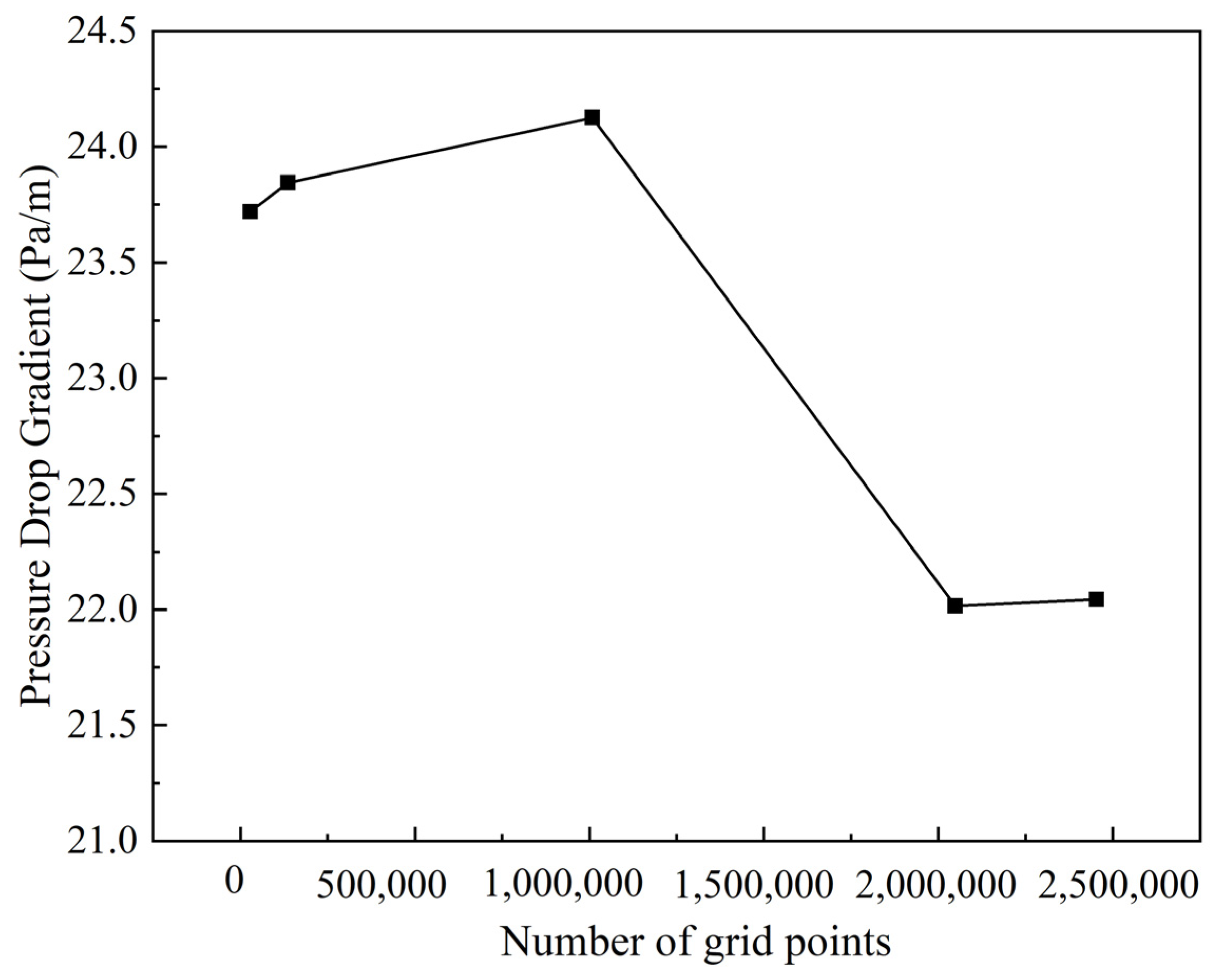
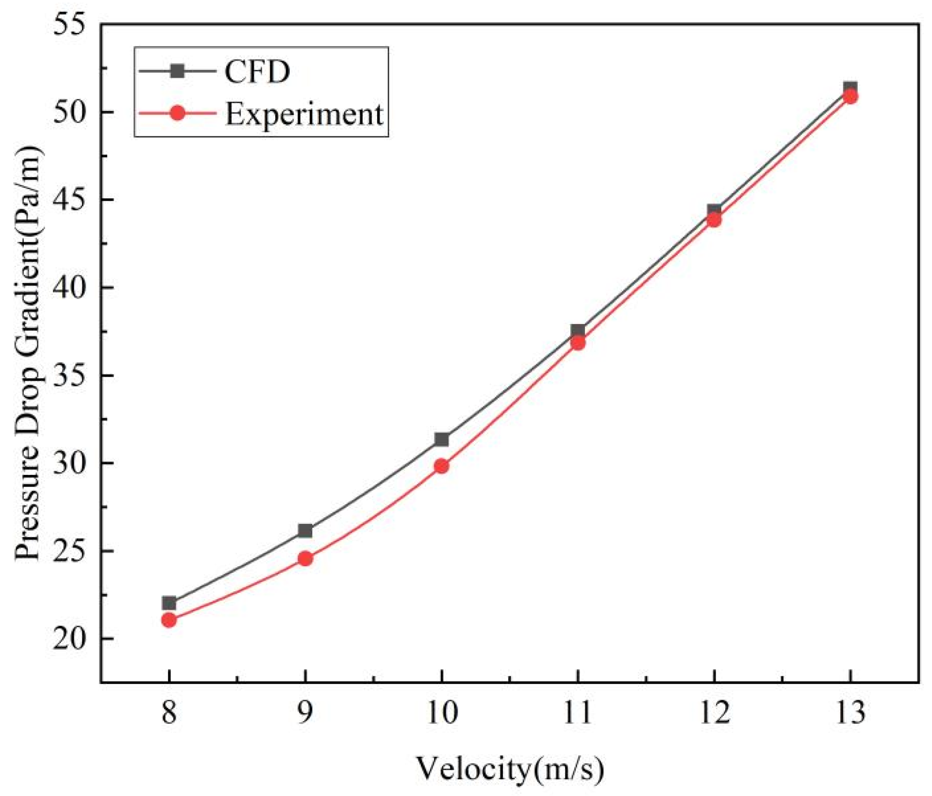
2.1.2. Model Validation

Before the numerical model is utilized for research purposes, it undergoes a rigorous validation process. This validation is conducted through simulation under conditions that mirror the experimental setup, with the pressure drop gradient serving as the benchmark for verification.
The validation of the numerical model was facilitated by a custom-designed experimental platform. A schematic representation of this experimental setup is depicted in Figure 1. The platform features an outer tube with an inner diameter of 110 mm, an inner tube with a diameter of 63 mm, and a total length of 8 m, to determine the inlet length for flow in an annulus based on the Equations (18) and (19); for an 8 m length, the inlet section requires 2.25 m and the outlet requires 1.1 m, meeting the requirements for fully developed flow. For the inlet length (Lin) of the annular flow [24,25].
L i n = 50 D o D i
For the outlet length (Lout) of the annular flow [26],
L o u t = 4.4 Re 1 6 D o D i
After the required lengths for the inlet and outlet are determined, the middle section, where the flow is fully developed, is used as the experimental section for measurement [27].
The flow rate adjustment capability was within the range of 8–13 m/s. The properties of the fluid were as follows: the density of air was approximately 1.18 kg/m3, the kinematic viscosity was approximately 185.5 mPa·s, and the air temperature was 30 °C. The Reynolds number range was between 22,900 and 37,213. The setup included a flowmeter (Model LUGB-100-TD-C, with a measuring range of 90–600 m3/h and an accuracy class of 1.0, manufactured by Dotory Automation Equipment Co., Ltd., Shangdong, China), a data acquisition system (Model DAM3055N, with an accuracy of one in a thousand and a resolution of 16 bits, manufactured by Aertech Technology Co., Ltd., Beijing, China), and a differential pressure transmitter (Model HY-130, with an accuracy of 0.25% FS and a measuring range of 1–5 kPa, manufactured by Shanghai Huanyu Automation Equipment Co., Ltd., Shanghai, China). The differential pressure transmitter was utilized to accurately measure the annular pressure drop. The numerical simulation was configured to replicate these exact experimental conditions.
Before the experiment commenced, the differential pressure transmitter was zeroed, and the data acquisition system was also zeroed and calibrated. The experiment involved measuring the fluid’s pressure drop within a range of 5 m from the inlet and 1.5 m from the outlet. The control fan for flow velocity was calibrated to establish a correlation between the frequency of the Variable-Frequency Drive (VFD) and the flow rate, enabling precise flow velocity control and adjustment of the fan through the VFD. The experiment was conducted with flow velocities ranging from 8 to 13 m/s, corresponding to a Reynolds number between 22,900 and 37,213. The eccentric device was calibrated by adjusting its height, with the eccentric distance adjustable within a range of −0.9 to 0.9. After the initial conditions were set, pressure drop data were measured and recorded in the experimental section. All operating conditions were covered by replacing either the inner tube with a roughness of 0.25 mm or the outer tube with a roughness of 1 mm.
Repetitive experiments were conducted on both smooth and rough pipelines based on the above experimental conditions, with each operating condition being tested three times. The experimental results are shown in Figure 2, and the analysis is presented in Table 1.
From the analysis in Table 1, it can be concluded that the overall uncertainty estimate (based on the average of standard deviations) for the pressure drop in smooth tubes is approximately 1.14. The overall uncertainty estimate (based on the average of standard deviations) for the pressure drop in rough tubes is approximately 2.69.
Simulations of an annulus were conducted in ANSYS Fluent 19.0 software [28], utilizing the Finite Volume Method (FVM) as the basis. The “SIMPLE” algorithm was employed to address the coupling between pressure and velocity. The momentum, turbulent kinetic energy, and specific dissipation rate equations were solved using the Second-Order Upwind scheme. Notably, the convergence criteria for computational residuals were uniformly set to 10−5. At the inlet of the annulus, an inlet velocity boundary condition was imposed, whereas at the outlet, an atmospheric pressure boundary condition was applied. Regarding the dimensions of the computational domain, the outer tube had a diameter of 110 mm, the inner tube had a diameter of 65 mm, and the length was 6 m. Hexahedral meshing was adopted, with a y+ value of 0.9 at the center of the first grid layer adjacent to the wall. A mesh independence verification is illustrated in Figure 3. The roughness heights were set to 0.25 mm and 1 mm, with a roughness constant of 0.5. The settings for roughness were based on the ANSYS Fluent Users Guide: the roughness height (Ks) and roughness constant (Cs) need to be specified. For uniform sand roughness, the height of the sand grains can be directly used as Ks, and the roughness constant (Cs) is taken as 0.5.
When the number of grid points reaches 2,048,160 and 2,453,780, as illustrated in Figure 3, the pressure drop gradient stabilizes essentially. Consequently, to enhance computational efficiency, a grid size of 2,048,160 is adopted for subsequent research.
Employing the RANS model to simulate complex turbulence offers a commendable balance between simulation accuracy and computational efficiency [29]. In this study, RANS is leveraged to investigate turbulence within concentric annular pipes. The entire turbulence within the horizontal annulus is meticulously simulated using RANS. As illustrated in Figure 4, the strong agreement between our current results and experimental data underscores the dependability of the RANS model in predicting the pressure drop gradient.
Based on the aforementioned analysis, this paper adopts this model for all subsequent numerical simulation research endeavors. The parameter range for the subsequent research is determined based on practical engineering applications. Specific details are shown in Table 2.

3. Results and Discussion

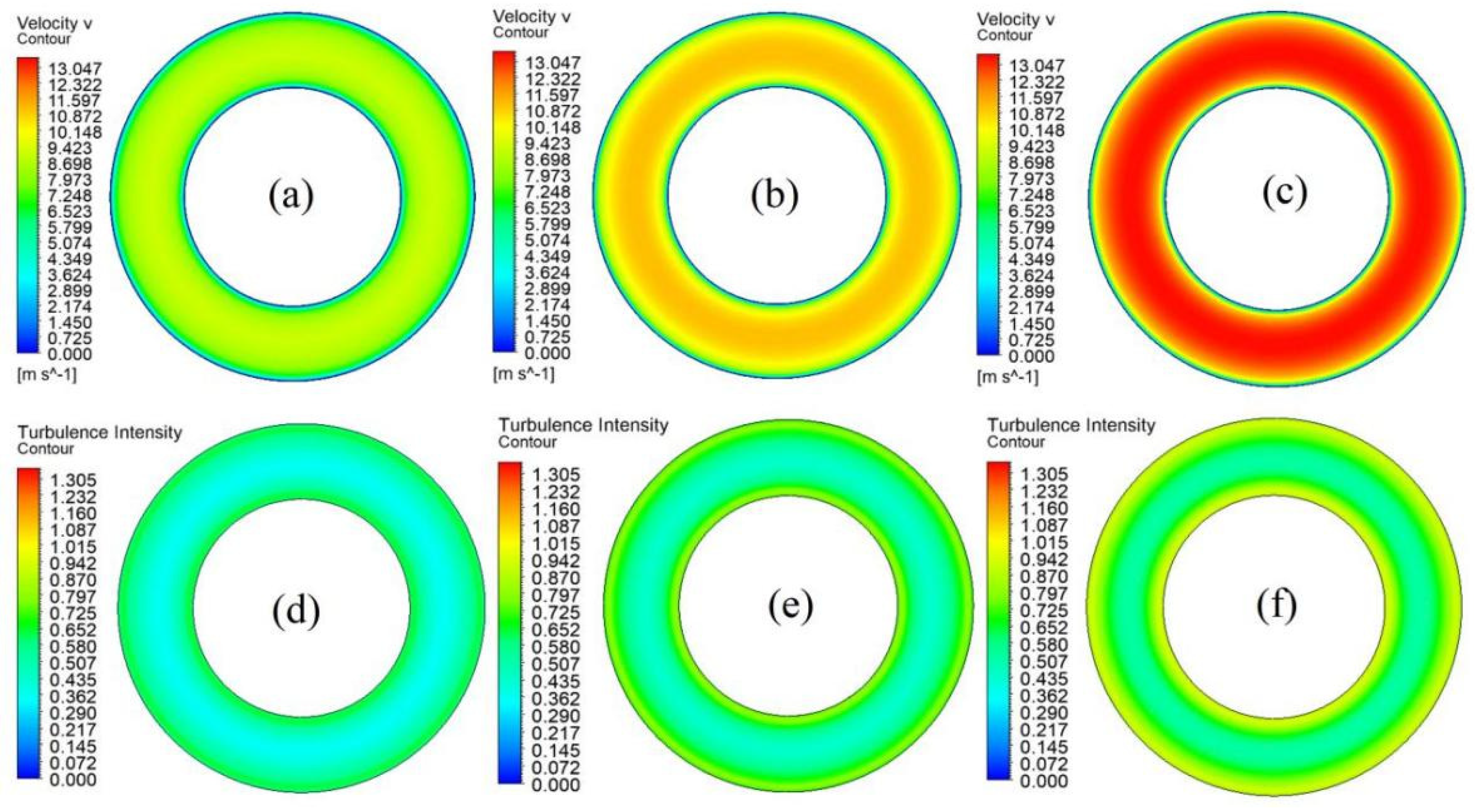
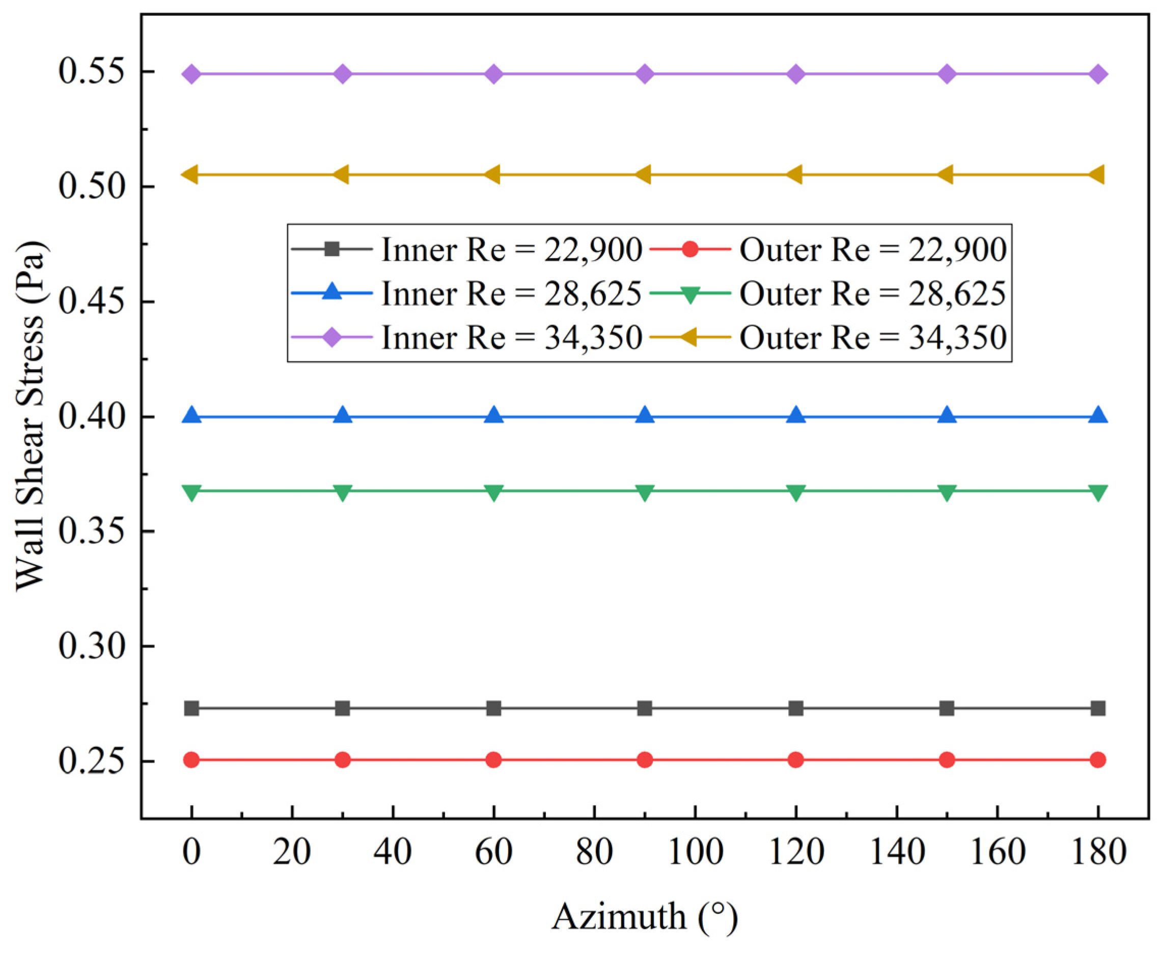
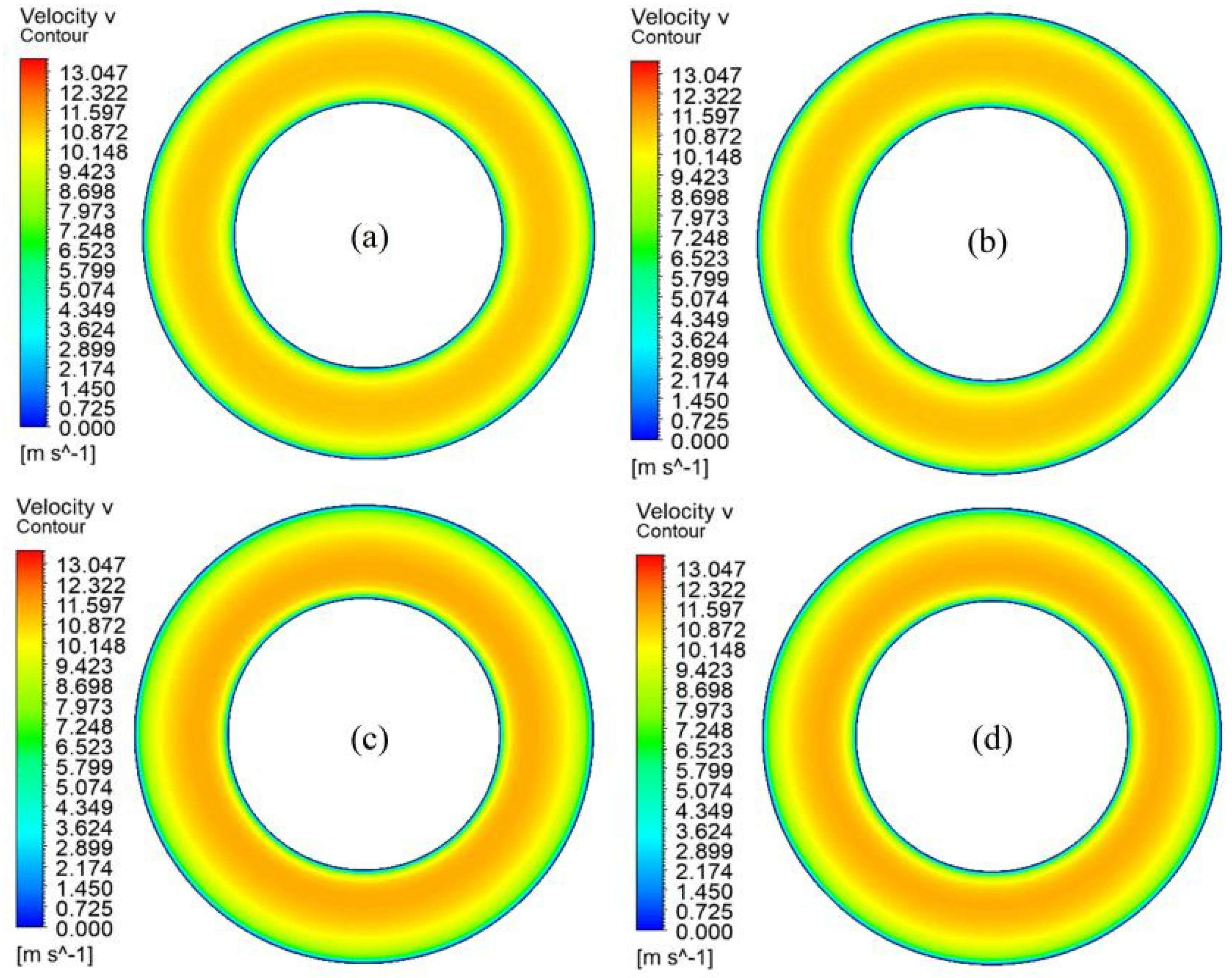
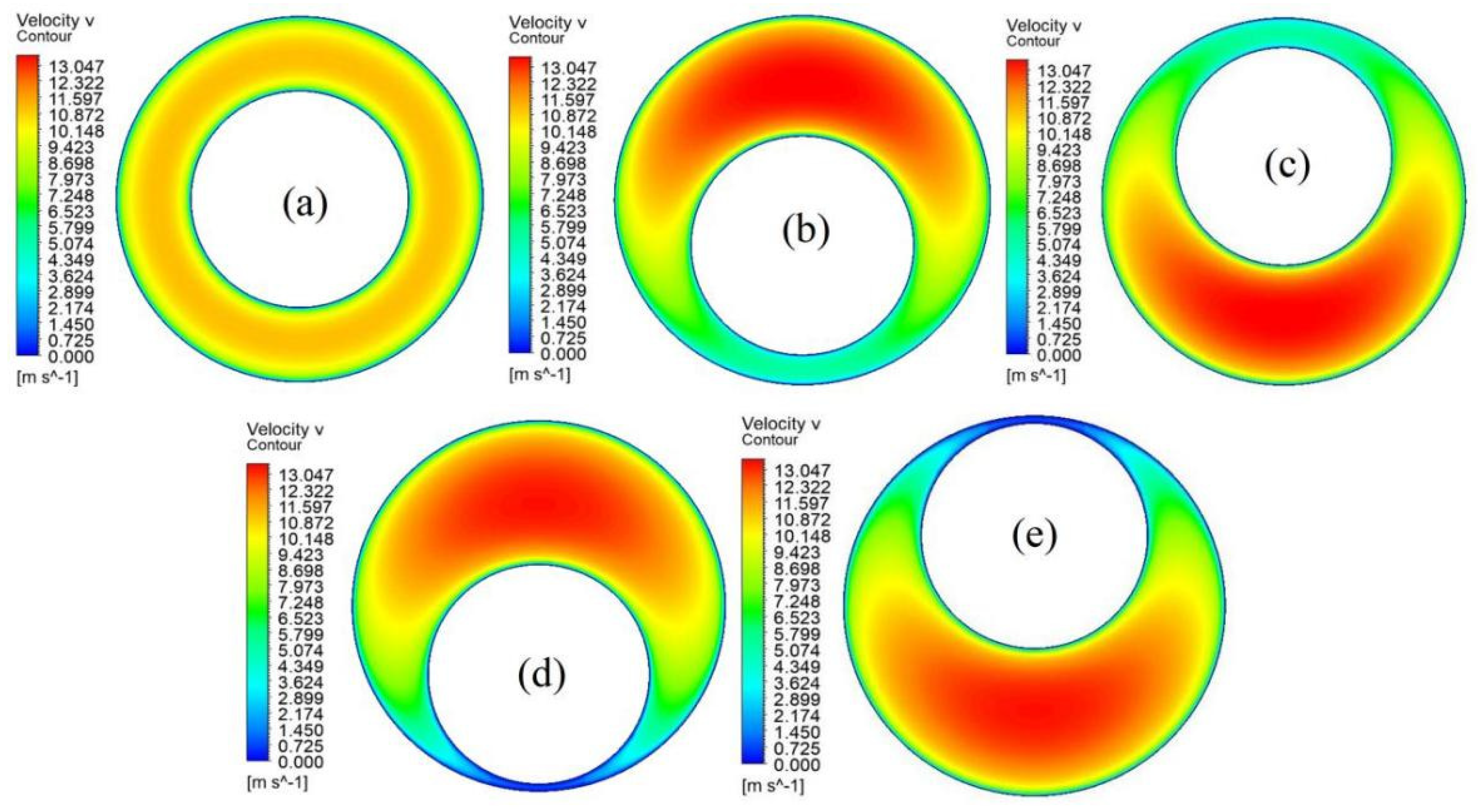
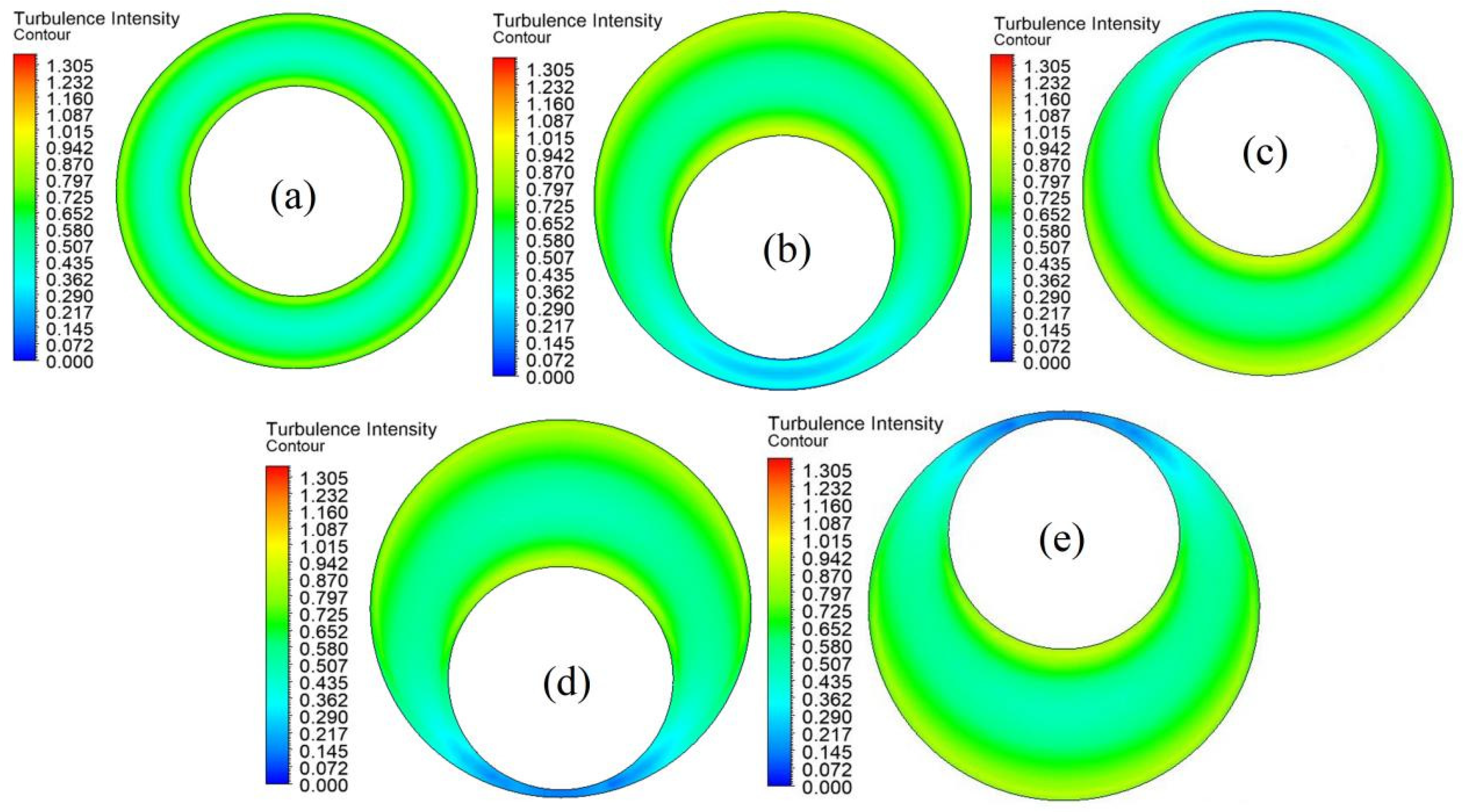
Turbulence and Wall Shear Stress Characteristics

Turbulence intensity serves as a quantitative measure of the intensity of turbulence development and the magnitude of turbulent kinetic energy. The more vigorous the turbulence, the greater its capacity for diffusion. Analyzing turbulence intensity provides valuable insights into the level of turbulence activity, which is crucial for understanding the macroscopic behavior of fluid flow.
In this paper, numerical simulation is employed to investigate the influence of flow velocity, eccentricity, and internal and external roughness on shear force under experimental conditions. The aim is to elucidate the variation in macroscopic pressure drop through the distribution of shear force. As a result, Figure 5 depicts the position of the extracted data on one side of the symmetrical circle.
As shown in Figure 6, in a concentric annulus, the velocity and turbulence intensity distributions exhibit central symmetry. However, the velocity is lowest near the wall and highest in the main flow region of the annulus. The distribution of turbulence intensity is the opposite, with the highest turbulence intensity near the wall and relatively lower values in the main flow region. As the inlet velocity increases, both the velocity and turbulence intensity within the annulus intensify. In concentric annulus flow, the distribution characteristics of velocity and turbulence intensity are primarily influenced by fluid dynamics principles, which can be explained through basic fluid mechanics principles. They exhibit central symmetry in a concentric annulus. The velocity peaks in the main flow region of the annulus because the resistance encountered in this region is relatively small, allowing the fluid to flow more smoothly. In contrast, near the wall, the velocity decreases significantly due to increased frictional resistance between the fluid and the wall. This velocity distribution is a typical characteristic of fluid flow in pipes or annuli. Turbulence intensity serves as an indicator of the degree of fluid flow disturbance. Near the wall, due to factors such as reduced velocity and wall roughness, fluid flow becomes more complex and turbulent, resulting in higher turbulence intensity. In the main flow region, however, the higher velocity and relatively smooth flow lead to lower turbulence intensity. This distribution of turbulence intensity aids in understanding energy dissipation and mixing processes in fluid flow within an annulus. When the inlet velocity increases, both the velocity and turbulence intensity within the annulus correspondingly intensify. This is because an increased inlet velocity means more kinetic energy is carried into the annulus by the fluid. This additional kinetic energy is converted into fluid velocity, resulting in an overall increase in velocity throughout the annulus. Simultaneously, the increased velocity enhances friction between the fluid and the wall, as well as interactions within the fluid itself, leading to an increase in turbulence intensity. These changes are common phenomena in fluid dynamics, reflecting the sensitivity of fluid flow states to external conditions. Additionally, it is worth noting that the increase in turbulence intensity is not only related to velocity but also influenced by various factors such as annulus geometry and wall conditions. Therefore, in practical applications, these factors need to be comprehensively considered to accurately predict and regulate the velocity and turbulence intensity distributions within an annulus.
As shown in Figure 7, when the Reynolds number reaches 28,625, compared to a Reynolds number of 22,900, the wall shear force of the inner and outer pipes increases by 46.5% and 46.7%, respectively. Similarly, at a Reynolds number of 34,350, compared to 22,900, the wall shear force of the inner and outer pipes surges by 101.1% and 101.6%, respectively. When analyzed in conjunction with the contour plots of turbulence intensity, it becomes apparent that as the Reynolds number increases, there is a notable enhancement in turbulence intensity near the wall. This indicates an intensification of turbulence activity in the vicinity of the wall, which serves as the primary factor contributing to the increase in wall shear force for both the inner and outer pipes. Meanwhile, as illustrated in Figure 6 and Figure 7, the turbulence characteristics and wall shear force exhibit central symmetry at different Reynolds numbers.
Table 3 presents the four operating conditions resulting from variations in the smoothness and roughness of the inner and outer walls of the annulus. The contour maps of annulus flow velocity and turbulence intensity obtained from numerical simulations are shown in Figure 8 and Figure 9. It can be seen from Figure 8 that the changes in velocity distribution are not readily apparent. However, upon close inspection, it can be observed that as the transition from smooth tubes to rough tubes takes place, the velocity near the wall decreases, resulting in a narrowing of the annular zone in the mainstream area. As depicted in Figure 9, the numerical simulation results indicate that surface roughness amplifies the turbulence intensity near the wall, implying an increase in turbulent activity. With the increase in roughness of the inner tube, the turbulence intensity on the inner wall significantly rises, accompanied by a concurrent increase on the outer wall. Conversely, when the outer tube surface is rough, it also results in an elevation of turbulence intensity on the inner wall. As the roughness of both the inner and outer tubes escalates, the disparity in turbulence intensity becomes increasingly notable. Therefore, the augmentation in roughness leads to an overall increase in turbulence intensity levels.
From Table 4, an interesting observation can be drawn in Case 2 when comparing the wall shear stress between the inner and outer tubes under the condition of an inner tube roughness of 0.25 mm. In this scenario, compared to the smooth tubes in Case 1, the wall shear stress of the rough inner tube increased significantly by 25%. Simultaneously, the wall shear stress of the outer tube also increased by a more modest 3%. The difference in the magnitude of the increase in wall shear stress highlights the impact of inner tube roughness on the shear stress in adjacent tubes. In Case 3, under the condition of an outer tube roughness of 1 mm, compared to the smooth tubes in Case 1, the wall shear stress of the rough outer tube surged by 107.6%, and the wall shear stress of the inner tube also increased significantly by 17.3%. This further proves that a rough outer tube can affect the wall shear stress of the adjacent inner tube. In Case 4, when the roughness values of the inner and outer tubes were 0.25 mm and 1 mm, respectively, compared to the smooth tubes in Case 1, the wall shear stress of the rough inner tube increased significantly by 48.3%, and the wall shear stress of the outer tube increased astonishingly by 113.3%. This significant increase underscores that an overall increase in roughness enhances the wall shear stress in both inner and outer tubes, which is attributed to the interaction between roughness and the flowing fluid, leading to enhanced turbulence intensity and a profound impact on wall shear stress, as can be seen in Figure 9. The difference in the magnitude of increase in wall shear stress between the inner and outer tubes further reveals the complex interactions among fluid dynamics, annulus geometry, and surface roughness within annulus systems. These findings remind us that, when designing and optimizing such systems, the roughness of both inner and outer tubes must be carefully considered, as they have a significant impact on fluid turbulence levels, shear stress distribution, and ultimately the overall performance and efficiency of the system.
As shown in Figure 10 and Figure 11, the numerical simulation results show that the velocity distribution in the eccentric annulus is uneven, with an increase in velocity in the wide annulus and a decrease in velocity in the narrow annulus. This result makes the maximum time average axial velocity in the wide section increase with the increase in eccentricity, while the maximum time average axial velocity in the narrow section decreases with the increase in eccentricity, which is consistent with Dokhani’s results [11]. This distribution law is due to the increase in eccentricity; the flow in the narrow part of the annulus decreases, and the flow is transferred to the larger part of the annulus, resulting in an increase in velocity [13]. At the same time, the turbulence intensity in the wide annulus is also increasing, and that in the narrow annulus has decreased significantly.
The eccentricity will make the wall shear stress distribution of the inner and outer tubes uneven; the shear stress distribution in the large annulus will be greater than that in the concentric annulus, and the shear stress distribution in the small annulus will be less than that in the concentric annulus. With the increase in eccentricity, the average wall shear force decreases. As the annulus distance decreases, the difference between the inner and outer wall shear forces gradually decreases. It can be seen from Figure 10, Figure 11 and Figure 12 that the velocity distribution in the eccentric annulus depends on the annulus distance, and the velocity is the lowest at the minimum annulus, which is consistent with the reduction in the difference caused by the reduction in the average velocity in the annulus. Therefore, it also explains the result that the pressure drop decreases with the increase in eccentricity in the experiment.
As shown in Figure 12, when the eccentricity of the inner tube is equal to 0.6, the maximum increment and maximum reduction in the wall shear force of the inner tube relative to the center of the inner tube are 29% and −65.6%, respectively, and the maximum increment and maximum reduction in the wall shear force of the outer tube relative to the center of the inner tube are 25.3% and −64.2%, respectively. When the eccentricity of the inner tube is equal to 0.9, the maximum increment and maximum reduction in the wall shear force of the inner tube are 21% and −93.1% respectively, and the maximum increment and maximum reduction in the wall shear force of the outer tube are 15.6% and −92.6% respectively. When the eccentricity of the inner tube is equal to 0.6, the average shear force of the inner and outer tubes is reduced by 17.9% and 17.2% compared with the average shear force in the middle case. When the inner tube eccentricity is equal to 0.9, the average shear force of the inner and outer tubes is reduced by 36.4% and 35.7% compared with the average shear force in the middle case. Therefore, the increase in eccentricity leads to the reduction in the average shear force and further the reduction in pressure drop. The eccentricity shows the characteristics of turbulent drag reduction, and both the inner and outer tubes show drag reduction. The drag reduction of the inner tube is slightly larger than that of the outer tube, and the difference between the two tends to decrease in the narrow annulus.
As shown in Figure 10 and Figure 11, under both positive and negative eccentricity conditions, the velocity distribution and turbulence intensity distribution exhibit clear symmetry. Additionally, as illustrated in Figure 13, the wall shear stress under both positive and negative eccentric distances also displays symmetry. These symmetrical flow characteristics hold significant importance in the formulation of engineering measures.
Taking drilling as an example, understanding this symmetrical pattern is crucial for optimizing drilling operations and enhancing well performance. In drilling applications, eccentricity often arises due to various factors such as wellbore irregularities, casing wear, or the use of eccentric tools. Recognizing the symmetrical effects of eccentricity allows engineers to adjust drilling parameters, such as drill bit rotation speed and fluid flow rates, to mitigate potential issues related to uneven fluid flow and turbulence. This can lead to more efficient drilling, reduced equipment wear, and improved wellbore stability. Additionally, by incorporating this symmetry into drilling design and planning, engineers can anticipate and address potential challenges, ensuring safer and more cost-effective drilling operations. Overall, the recognition of this symmetry in drilling applications offers valuable insights for improving operational efficiency and well productivity.

4. Conclusions

This paper delves into the turbulence characteristics within the following ranges of operating parameters through numerical simulation methods: flow velocities of 8–13 m/s, Reynolds numbers of 22,900–37,213, eccentricity ratios ranging from −0.9 to 0.9, and four roughness conditions for both inner and outer pipes. The flow field characteristics studied, including flow velocity distribution, turbulence intensity, and wall shear stress, were obtained in the fully developed turbulent region. Based on this thorough analysis, the following conclusions can be drawn:
  • Across various Reynolds numbers, the wall shear force and turbulence characteristics display a distinct central symmetry, with the inner pipe experiencing a notably higher wall shear force compared to the outer pipe. As the Reynolds number intensifies, there is a corresponding augmentation in the wall shear force on both pipes, and the disparity between their wall shear forces widens as the Reynolds number increases.
  • Numerical simulations reveal that an escalation in the roughness of the inner pipe significantly amplifies the wall shear force acting upon it, while concurrently elevating the wall shear force on the outer pipe. Conversely, when the outer pipe’s roughness increases, the wall shear force on the inner pipe also undergoes an augmentation.
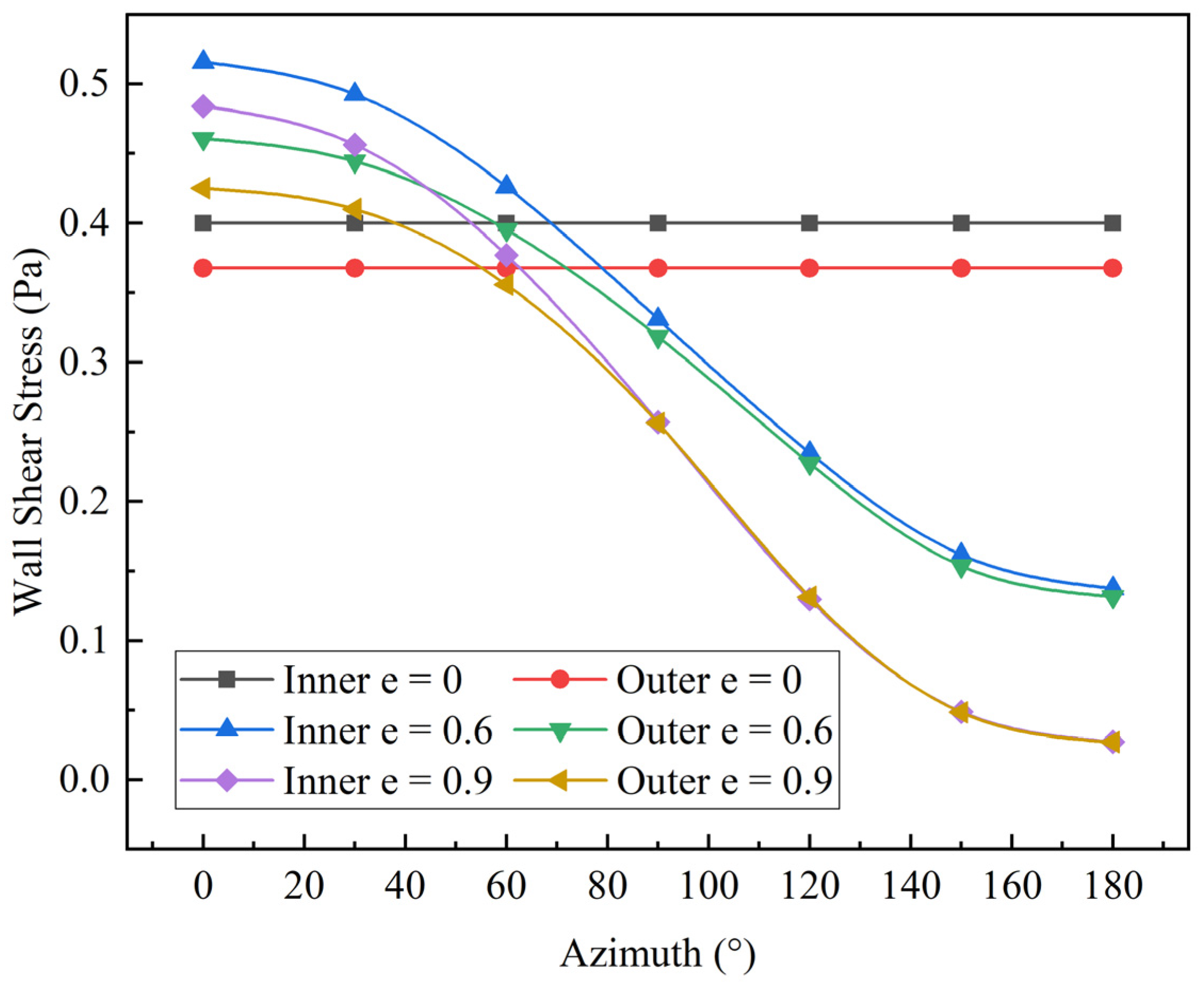
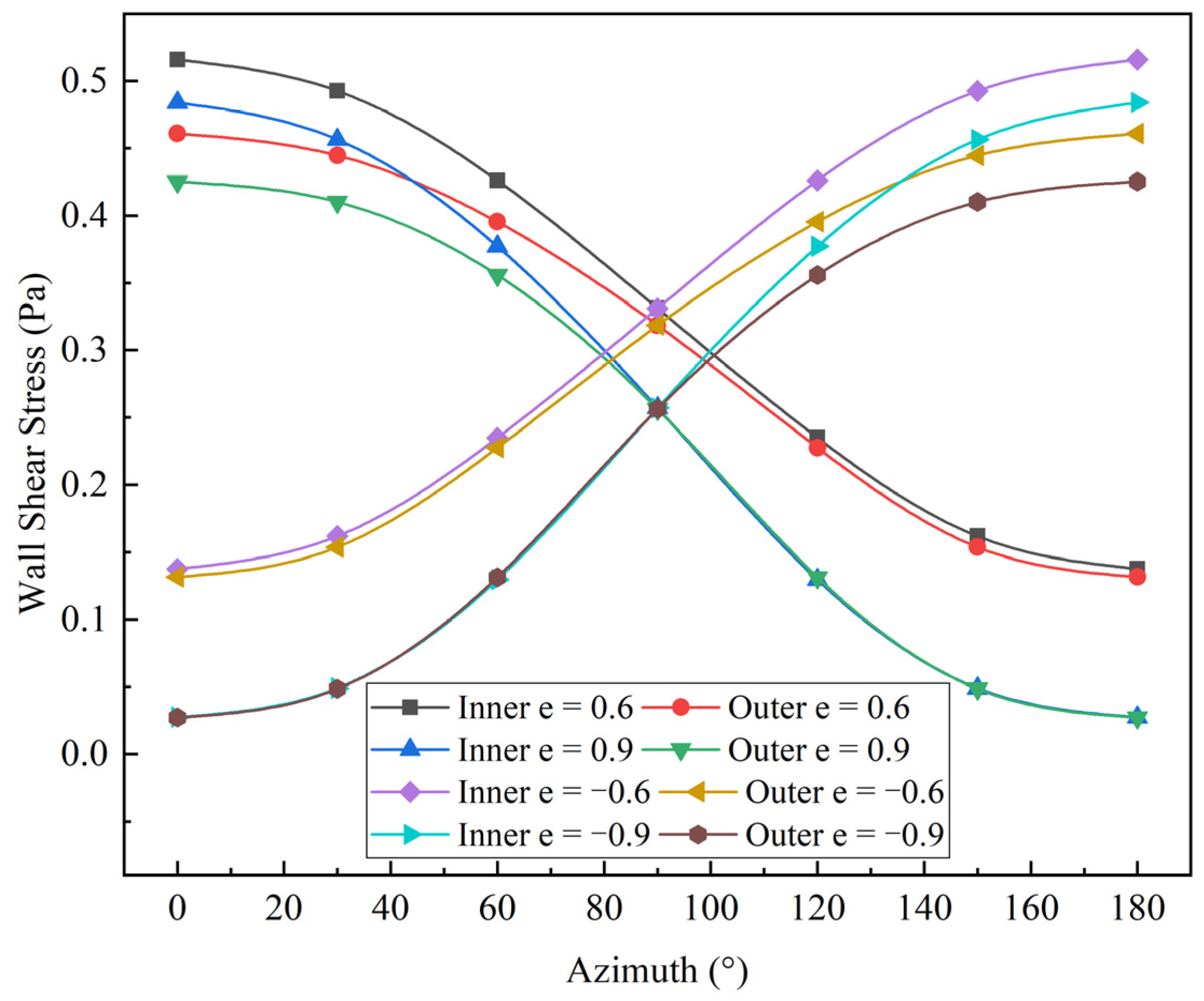
  • The introduction of eccentricity leads to an uneven distribution of wall shear force across both the inner and outer pipes. In larger annular spaces, the shear force distribution surpasses that observed in concentric configurations, whereas in smaller annular spaces, it diminishes. Notably, during instances of negative eccentricity, a reversal in this distribution pattern is evident. Furthermore, the wall shear force and turbulence characteristics exhibit axial symmetry, regardless of whether the eccentricity is positive or negative.

Author Contributions

Writing—original draft preparation, Y.S.; writing—review and editing, J.S.; visualization, J.Z.; supervision, Y.S.; project administration, J.Z.; writing—review and editing, supervision, funding acquisition, N.H. All authors have read and agreed to the published version of the manuscript.

Funding

This research was funded by the National Natural Science Foundation of China (grant numbers 41931179 and 42376232).

Data Availability Statement

No new data were created or analyzed in this study. The data that support the findings of this study are available on request from the corresponding author upon reasonable request.

Acknowledgments

The authors are grateful to the editor and the anonymous reviewers of this paper, especially the professors from the College of Civil Engineering and Mechanics, Lanzhou University, who provided inspiration and guidance for this paper.

Conflicts of Interest

The authors declare no conflicts of interest.

Nomenclature

ϕ i , ϕ i , φ i turbulent, time-averaged, and fluctuating variables in the RANS model, respectively
ui, ujtime-varying velocities in x, y, and z directions, respectively (m/s)
Ui, Ujtime-averaged velocities in x, y, and z directions, respectively (m/s)
υkinetic viscosity (m2/s)
kturbulent kinetic energy (m2/s2)
F1, F2blending functions in the turbulence model
Pkproduction of turbulent kinetic energy (m2/s3)
P ~ k modified production of turbulent kinetic energy (m2/s3)
Din, Doutinner and outer diameter of the annulus, respectively (m)
Re = ρUbD/μReynolds number based on bulk mean velocity
Ubbulk mean velocity (m/s)
μdynamic viscosity (Pa·s)
ρdensity (kg/m3)
Saverage shear strain rate (1/s)
sij, Sijaverage shear strain tensor for fluctuating and average velocity field, respectively (1/s)
U, Uvector and magnitude of velocity (m/s)
εviscous dissipation of turbulent kinetic energy (m2/s3)
υteddy viscosity (m2/s)
ωturbulent eddy frequency (1/s)
Rrepresents roughness
istands for inner pipe
ostands for outer pipe
eeccentricity

References

  1. Bagheri, E.; Wang, B.C.; Yang, Z. Influenceof domain size on direct numerical simulation of turbulent flow in a moderately curved concentric annular pipe. Phys. Fluids. 2020, 32, 065105. [Google Scholar] [CrossRef]
  2. Bagheri, E.; Wang, B.C. Effects of radius ratio on turbulent concentric annular pipe flow and structures. Int. J. Heat Fluid Flow. 2020, 86, 108725. [Google Scholar] [CrossRef]
  3. Xiong, X.; Rahman, A.M.; Zhang, Y. RANS Based Computational Fluid Dynamics Simulation of Fully Developed Turbulent Newtonian Flow in Concentric Annuli. J. Fluids Eng. 2016, 138, 091202. [Google Scholar] [CrossRef]
  4. Xiong, X.; Zhang, Y.; Rahman, A.M. Reynolds-Averaged Simulation of the Fully Developed Turbulent Drag Reduction Flow in Concentric Annuli. J. Fluids Eng. 2020, 142, 101209. [Google Scholar] [CrossRef]
  5. Zhang, Y.; Li, N. Numerical Simulation of Turbulent Flow for non-Newtonian Fluid in two kinds Complex Annulus Channel. J. Phys. Conf. Ser. 2021, 1985, 012062. [Google Scholar] [CrossRef]
  6. Bekiri, F.; Benchabane, A. Numerical study of drilling fluids flow in drilling operation with pipe rotation. Mater. Today Proc. 2021, 49, 950–954. [Google Scholar] [CrossRef]
  7. Najafabadi, M.F.; Farhadi, M.; Rostami, H.T. Numerically analysis of a Phase-change Material in concentric double-pipe helical coil with turbulent flow as thermal storage unit in solar water heaters. J. Energy Storage 2022, 55, 105712. [Google Scholar] [CrossRef]
  8. Himanshu, O.P.; Kurmi, S.J.; Tyagi, S.K. Performance assessment of an improved gasifier stove using biomass pellets: An experimental and numerical investigation. Sustain. Energy Technol. Assess. 2022, 53, 102432. [Google Scholar] [CrossRef]
  9. Motaman, S.; Eltaweel, M.; Herfatmanesh, M.R.; Knichel, T.; Deakin, A. Numerical analysis of a flywheel energy storage system for low carbon powertrain applications. J. Energy Storage 2023, 61, 106808. [Google Scholar] [CrossRef]
  10. Jing, J.; Huang, W.; Karimov, R.; Sun, J.; Li, Y. Numerical investigation on oil-water flow characteristics and construction optimization for novel wellbore lubrication fitting. AIP Adv. 2024, 14, 035306. [Google Scholar] [CrossRef]
  11. Dokhani, V.; Ma, Y.; Li, Z. An Accurate Model for Prediction of Turbulent Frictional Pressure Loss of Power-Law Fluids in Eccentric Geometries. SPE Drill. Complet. 2021, 36, 913–930. [Google Scholar] [CrossRef]
  12. Haciislamoglu, M.; Langlinais, J. Non-Newtonian Flow in Eccentric Annuli. J. Energy Resour. Technol. 1990, 112, 163–169. [Google Scholar] [CrossRef]
  13. Erge, O.; Ozbayoglu, E.M.; Miska, S.Z.; Yu, M.; Takach, N.; Saasen, A.; May, R. CFD Analysis and Model Comparison of Annular Frictional Pressure Losses While Circulating Yield Power Law Fluids. In Proceedings of the SPE Bergen One Day Seminar, Bergen, Norway, 22 April 2015. [Google Scholar]
  14. Ferroudji, H.; Hadjadj, A.; Haddad, A.; Ofei, T.N. Numerical study of parameters affecting pressure drop of power-law fluid in horizontal annulus for laminar and turbulent flows. J. Pet. Explor. Prod. Technol. 2019, 9, 3091–3101. [Google Scholar] [CrossRef]
  15. Ferroudji, H.; Hadjadj, A.; Ofei, T.N.; Rahman, M.A.; Hassan, I.; Haddad, A. CFD method for analysis of the effect of drill pipe orbital motion speed and eccentricity on the velocity profiles and pressure drop of drilling fluid in laminar regime. Petrol Coal 2019, 61, 1241–1251. [Google Scholar]
  16. Ferroudji, H.; Hadjadj, A.; Rahman, M.A.; Hassan, I.; Ofei, T.N.; Haddad, A. The impact of orbital motion of drill pipe on pressure drop of non-Newtonian fluids in eccentric annulus. J. Adv. Res. Fluid Mech. Therm. Sci. 2020, 65, 94–108. [Google Scholar]
  17. Belimane, Z.; Hadjadj, A.; Ferroudji, H.; Rahman, M.A.; Qureshi, M.F. Modeling surge pressures during tripping operations in eccentric annuli. J. Nat. Gas Sci. Eng. 2021, 96, 104233. [Google Scholar] [CrossRef]
  18. Liu, Y.; Mitchell, T.; Upchurch, E.R.; Ozbayoglu, E.M.; Baldino, S. Investigation of Taylor bubble dynamics in annular conduits with counter-current flow. Int. J. Multiph. Flow. 2024, 170, 104626. [Google Scholar] [CrossRef]
  19. Rushd, S.; Shazed, A.R.; Faiz, T. CFD Simulation of pressure losses in eccentric horzontal wells. In Proceedings of the SPE Middle East Oil & Gas Show and Conference, Manama, Bahrain, 6 March 2017. [Google Scholar]
  20. Francois, G.S. About Boussinesq’s Turbulent Viscosity Hypothesis: Historical Remarks and a Direct Evaluation of Its Validity. C.R. Mec. 2007, 335, 617–627. [Google Scholar]
  21. Menter, F.R. Two-Equation Eddy-Viscosity Turbulence Models for Engineering Applications. AIAA J. 1994, 32, 1598–1605. [Google Scholar] [CrossRef]
  22. Menter, F.R. Multiscale Model for Turbulent Flows. In Proceedings of the 24th Fluid Dynamics Conference, American Institute of Aeronautics and Astronautics, Orlando, FL, USA; 1993. [Google Scholar]
  23. Keshmiri, A.; Uribe, J.; Shokri, N. Benchmarking of Three Different CFD Codes in Simulating Natural, Forced and Mixed Convection Flows. Int. J. Comput. Method. 2015, 67, 1324–1351. [Google Scholar] [CrossRef]
  24. Knudsen, J.G.; Katz, D.V. Fluid Dynamics and Heat Transfer. Phys. Today 1958, 12, 40–44. [Google Scholar] [CrossRef]
  25. Chadwick, A.; John, M.; Martin, B. Hydraulics in Civil and Environmental Engineering, 5th ed.; CRC Press: Boca Raton, FL, USA, 2013. [Google Scholar]
  26. White, F.M. Fluid Mechanics, 7th ed.; McGraw-Hill Series in Mechanical Engineering: New York, NY, USA, 2011. [Google Scholar]
  27. Huque, M.M.; Butt, S.; Zendehboudi, S.; Imtiaz, S. Systematic sensitivity analysis of cuttings transport in drilling operation using computational fluid dynamics approach. J. Nat. Gas Sci. Eng. 2020, 81, 103386. [Google Scholar] [CrossRef]
  28. Ansys Inc. ANSYS Fluent 19.0. ANSYS Fluent Users Guide; Ansys Inc.: Canonsburg, PA, USA, 2019. [Google Scholar]
  29. Kalitzin, G.; Medic, G.; Iaccarino, G.; Durbin, P. Near-Wall Behavior of RANS Turbulence Models and Implications for Wall Functions. J. Comput. Phys. 2005, 204, 265–291. [Google Scholar] [CrossRef]
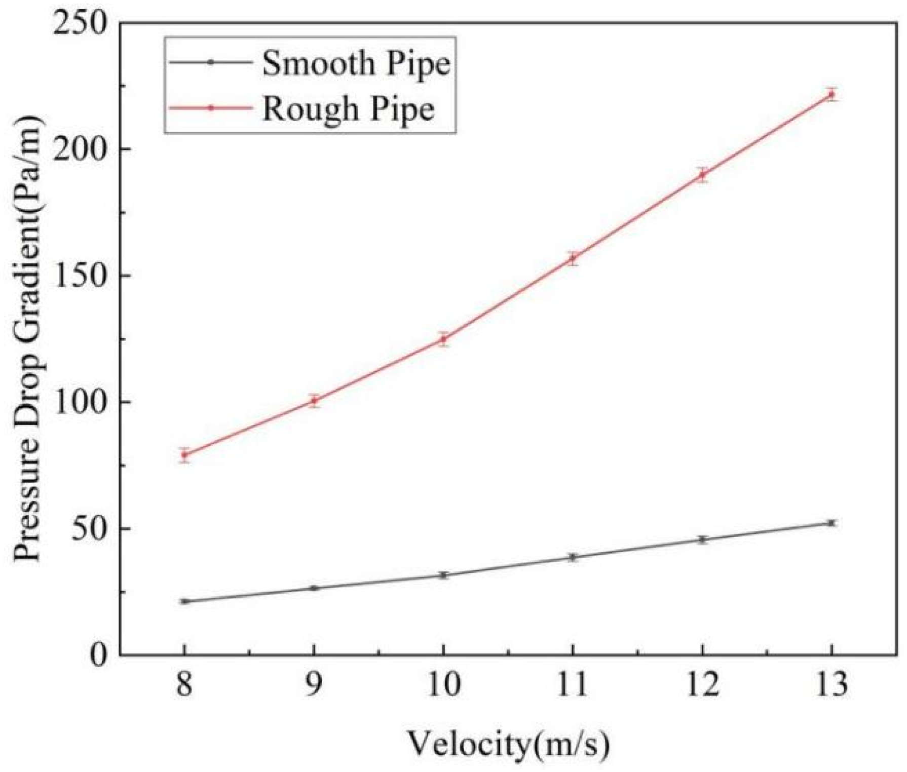
Figure 1. Schematic diagram of the experimental setup: 1, electric motor; 2, frequency converter; 3, flowmeter; 4, high-pressure blower; 5, eccentric device; 6, outer annulus pipe; 7, inner annulus pipe; 8, differential pressure transmitter; 9, data acquisition system.
Symmetry 17 00409 g001
Figure 2. Verification of experimental reproducibility.
Symmetry 17 00409 g002
Figure 3. The study of grid independence.
Symmetry 17 00409 g003
Figure 4. Numerical model validation.
Symmetry 17 00409 g004
Figure 5. Positions for data extraction in different directions.
Symmetry 17 00409 g005
Figure 6. Contour of annular velocity, turbulence intensity at different Reynolds numbers. Re = 22,900 (a,d), Re = 28,625 (b,e), Re = 34,350 (c,f).
Symmetry 17 00409 g006
Figure 7. Wall shear stress distribution of inner and outer tubes at different Reynolds numbers.
Symmetry 17 00409 g007
Figure 8. Contour of annular velocity under four working conditions: (a) Case 1, (b) Case 2, (c) Case 3, (d) Case 4.
Symmetry 17 00409 g008
Figure 9. Contour of annular turbulence intensity under four working conditions: (a) Case 1, (b) Case 2, (c) Case 3, (d) Case 4.
Symmetry 17 00409 g009
Figure 10. Cloud chart of annular velocity under different eccentricities: (a) e = 0, (b) e = 0.6, (c) e = −0.6, (d) e = 0.9, (e) e = −0.9.
Symmetry 17 00409 g010
Figure 11. Cloud chart of annular turbulence intensity under different eccentricities: (a) e = 0, (b) e = 0.6, (c) e= −0.6, (d) e = 0.9, (e) e = −0.9.
Symmetry 17 00409 g011
Figure 12. Comparison of wall shear stress of inner and outer tubes under different eccentricities.
Symmetry 17 00409 g012
Figure 13. Distribution of wall shear stress under positive and negative eccentricity.
Symmetry 17 00409 g013
Table 1. Experimental results of mean and variance of pressure drop at different flow rates.
Velocity (m/s)Smooth TubeRough Tube
Mean ± Standard DeviationMean ± Standard Deviation
821.17 ± 0.7179.06 ± 2.81
926.37 ± 0.62100.46 ± 2.51
1031.52 ± 1.31124.85 ± 2.73
1138.65 ± 1.50156.78 ± 2.60
1245.61 ± 1.58189.82 ± 2.82
1352.28 ± 1.09221.58 ± 2.58
Table 2. Operating condition parameters and values for numerical simulation.
ParametersValue
Velocity (m/s)8, 10, 12
Roughness (mm)0, 0.25 (inner); 0, 1 (outer)
Eccentricity0, 0.6, 0.9
Table 3. Four operating conditions of the inner and outer tubes.
Parameter TubeCase 1Case 2Case 3Case 4
Roughness (mm)Inner (Ri) 00.2500.25
Outer (Ro) 0011
Table 4. The circumferential distribution of wall shear stress on both inner and outer pipes under four operating conditions.
Parameter TubeCase 1Case 2Case 3Case 4
wall shear stress (Pa)inner 0°0.40.50.470.59
inner 30°0.40.50.470.59
inner 60°0.40.50.470.59
inner 90°0.40.50.470.59
inner 120°0.40.50.470.59
inner 150°0.40.50.470.59
inner 180°0.40.50.470.59
outer 0°0.370.380.760.78
outer 30°0.370.380.760.78
outer 60°0.370.380.760.78
outer 90°0.370.380.760.78
outer 120°0.370.380.760.78
outer 150°0.370.380.760.78
outer 180°0.370.380.760.78
Disclaimer/Publisher’s Note: The statements, opinions and data contained in all publications are solely those of the individual author(s) and contributor(s) and not of MDPI and/or the editor(s). MDPI and/or the editor(s) disclaim responsibility for any injury to people or property resulting from any ideas, methods, instructions or products referred to in the content.

