
Development and Engineering Applications of a Novel Mixture Distribution: Exponentiated and New Topp–Leone-G Families

 , ,
, ,
Abstract
:1. Introduction
2. Mixture of Exponentiated and New Topp Leone-G Family
2.1. General Properties of the Mixture of Exponentiated and New Topp–Leone-G Families
2.1.1. Quantile Function of the MENTL-G Family
2.1.2. Moments of the MENTL-G Family
- The series’ representation as ;
- The generalized binomial expansion for is a real non-integer
- Taylor expansion .
2.1.3. Moment-Generating Function of the MENTL-G Family
2.1.4. Order Statistics of the MENTL-G Family
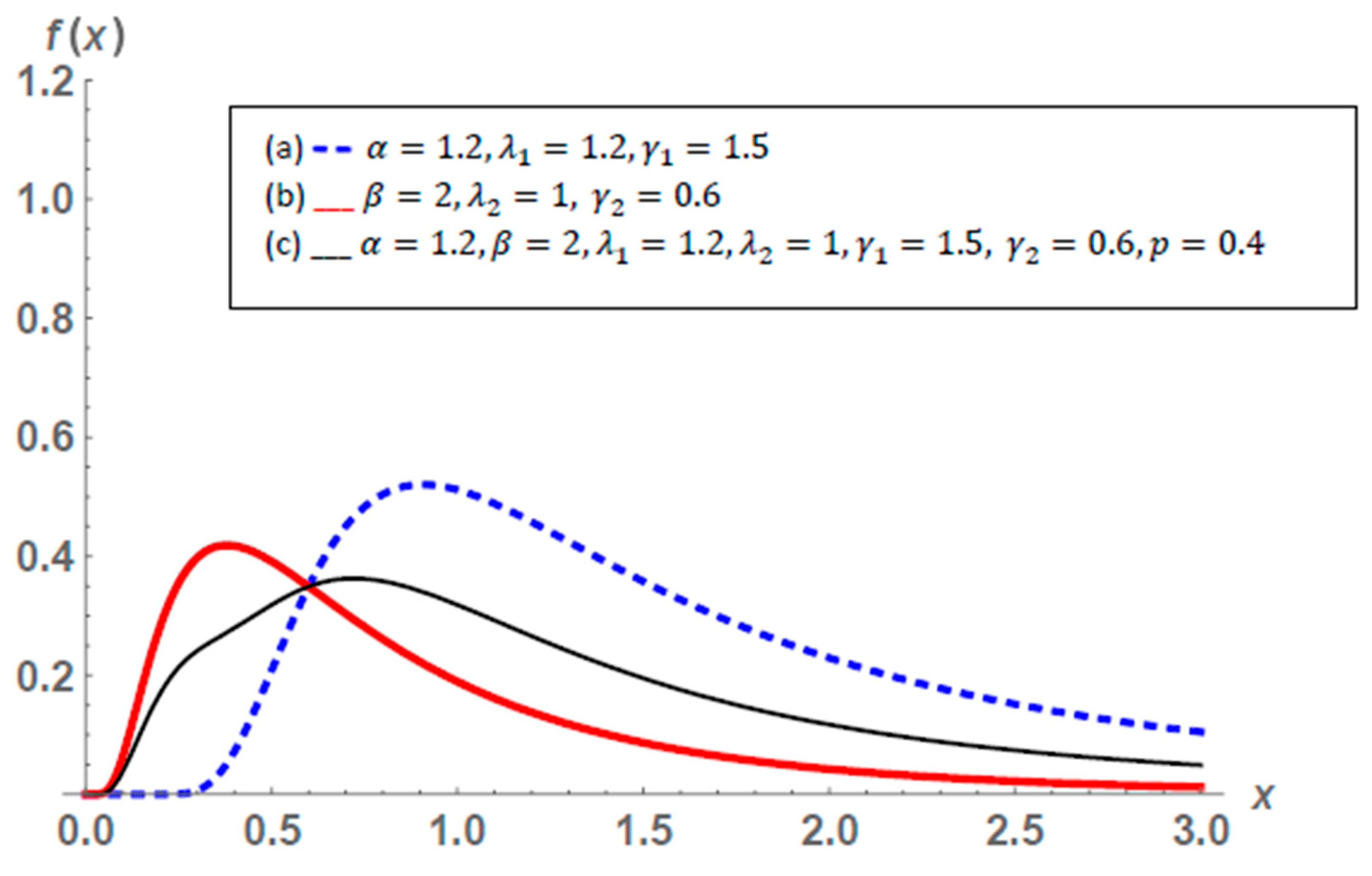
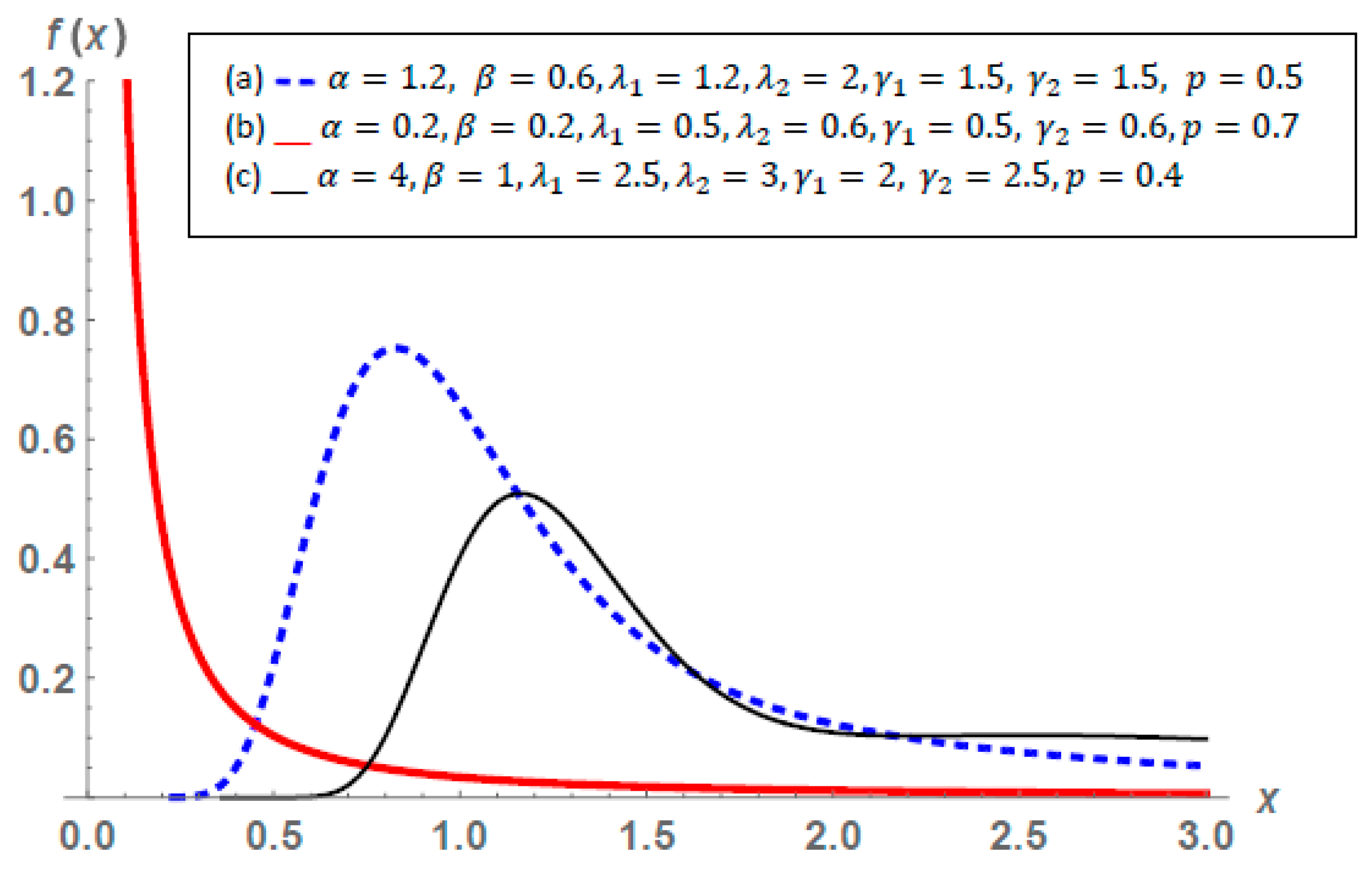
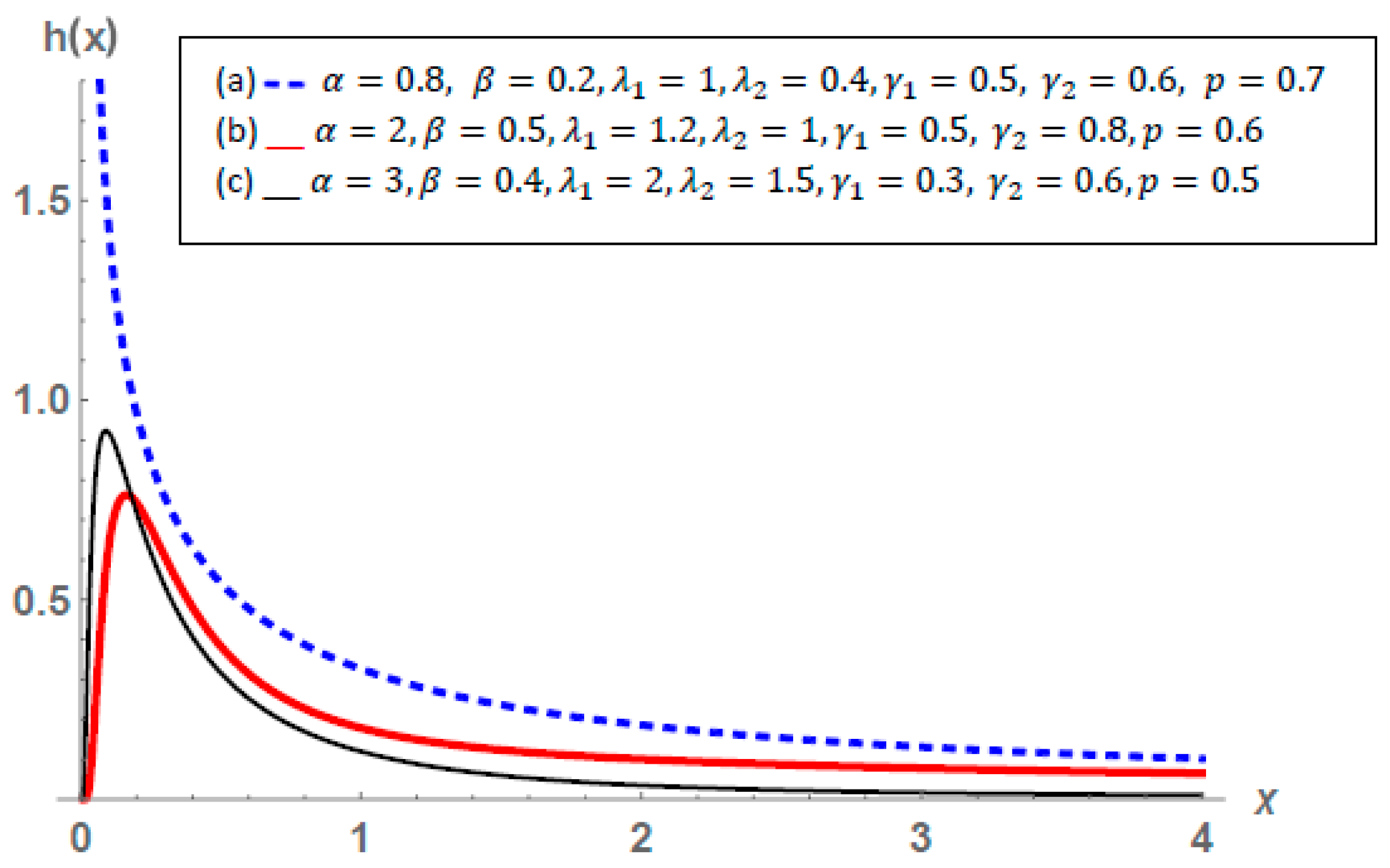
3. Mixture of Two Exponentiated New Topp–Leone Inverse Weibull Distribution
3.1. Description of the Distribution
3.2. Some Statistical Properties
3.2.1. Quantile Function
3.2.2. Moments
3.2.3. Moment-Generating Function
3.2.4. Distribution of Order Statistics
4. Estimation for Mixture of Two Exponentiated New Topp–Leone Inverse Weibull Distributions
4.1. Maximum Likelihood Estimation
4.2. Bayesian Estimation
- Bayesian estimation of mixture exponentiated new Topp–Leone inverse Weibull distribution under squared error loss function
- II.
- Bayesian estimation of mixture exponentiated new Topp–Leone inverse Weibull distribution under LINEX loss function
5. Numerical Results
5.1. Simulation Study
- The following steps are used to generate samples from the MENTL-IW distribution:
- II.
- The following steps are considered to generate samples for Bayes estimators under SE and LINEX loss functions from the MENTL-IW distribution:
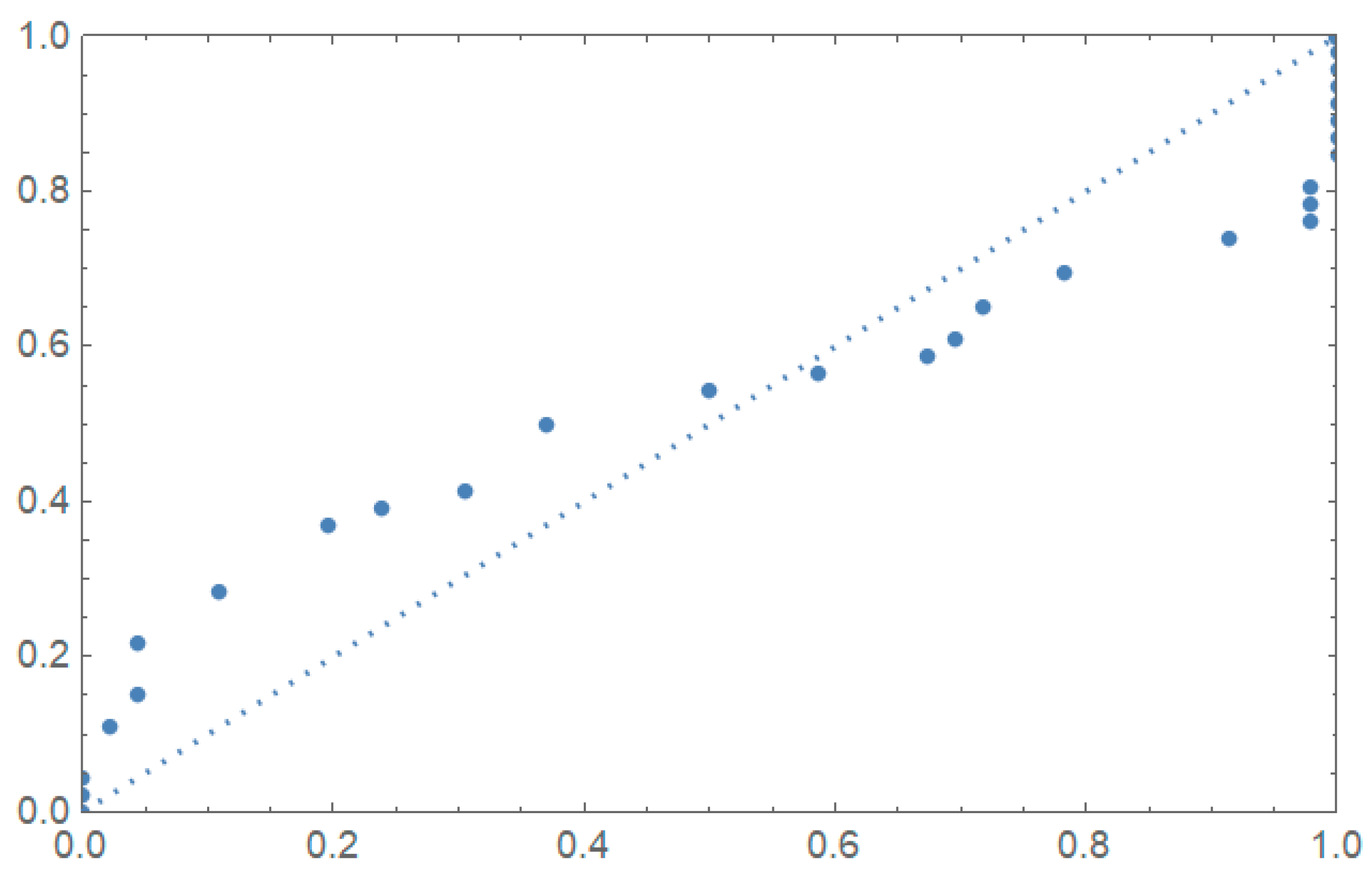
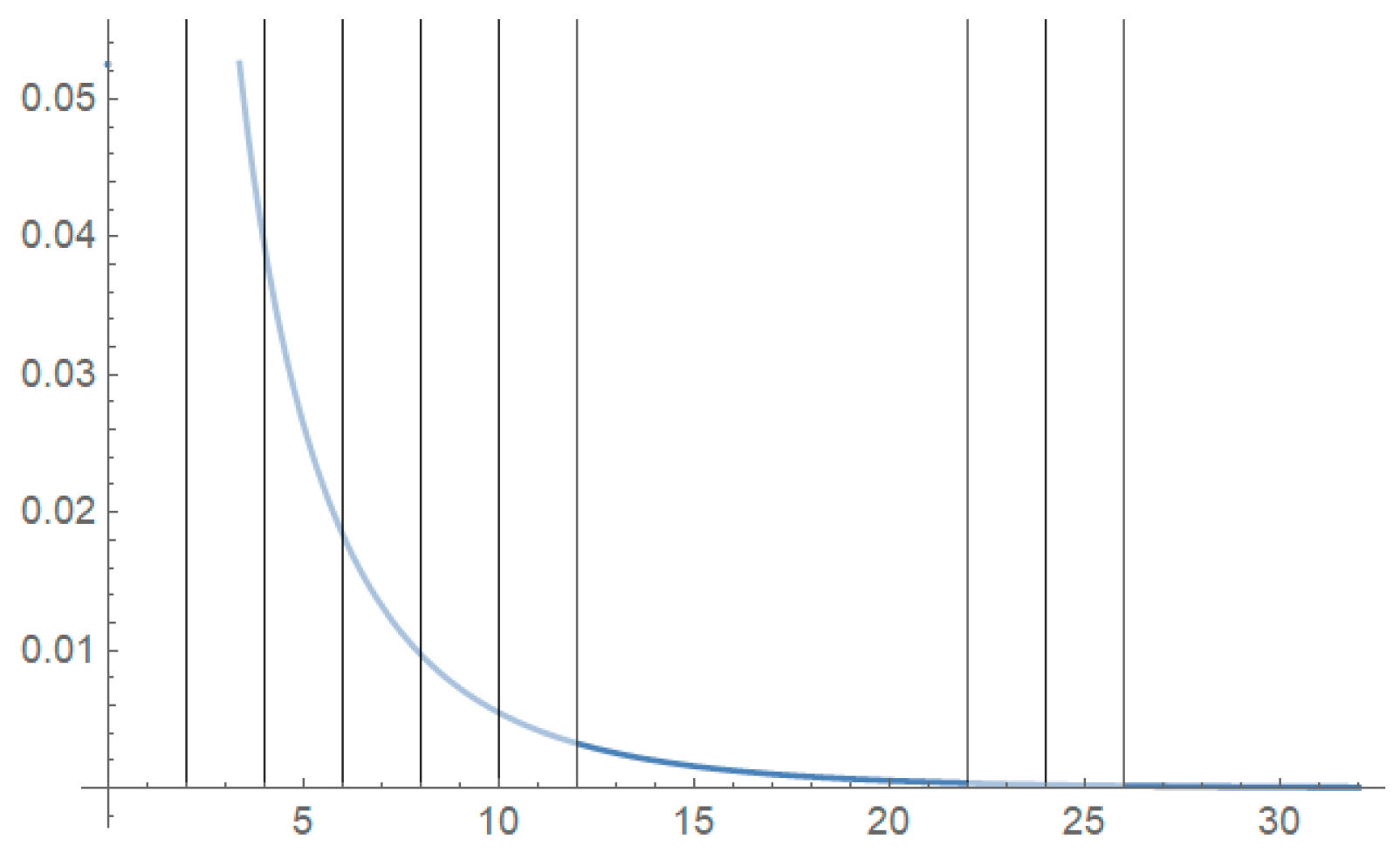
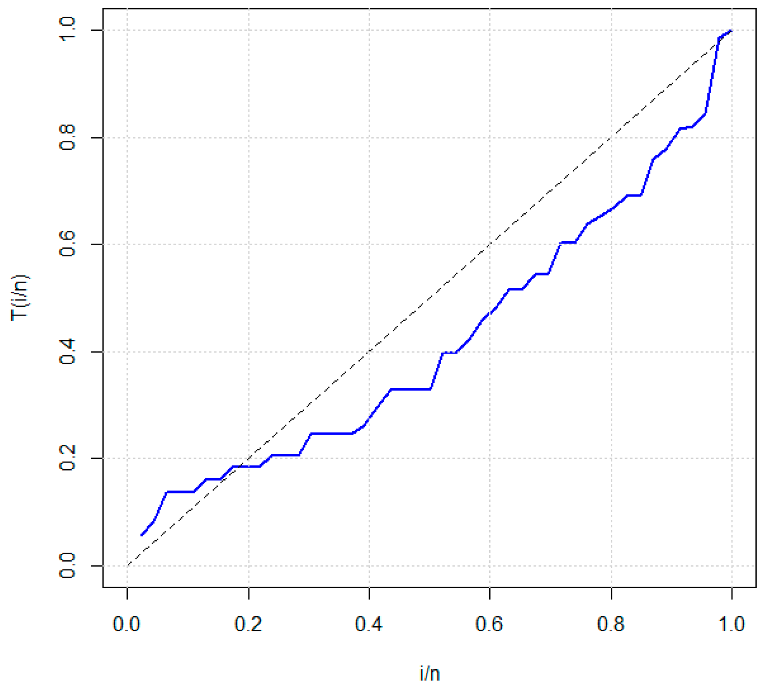
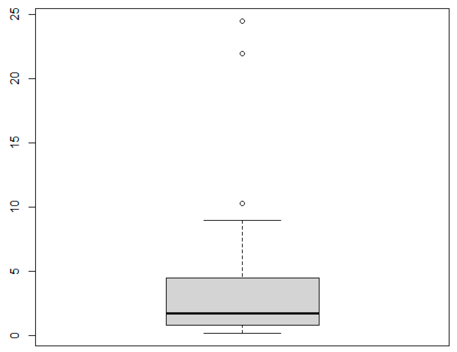
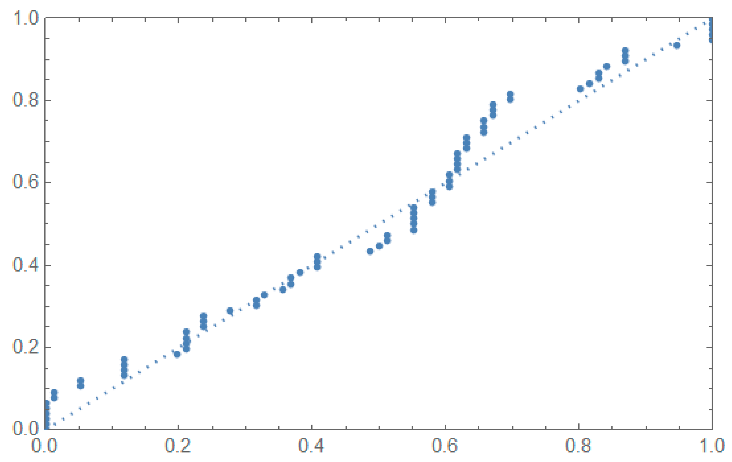
5.2. Applications
| 0.2, 0.3, 0.5, 0.5, 0.5, 0.6, 0.6, 0.7, 0.7, 0.7, 0.8, 0.8, 0.8, 1.0, 1.0, 1.0, 1.0, 1.1, 1.3, 1.5, 1.5, 1.5, 1.5, 2.0, 2.0, 2.2, 2.5, 2.7, 3.0, 3.0, 3.3, 3.3, 4.0, 4.0, 4.5, 4.7, 5.0, 5.4, 5.4, 7.0, 7.5, 8.8, 9.0, 10.3, 22.0 and 24.5. |
| 0.0251, 0.0886, 0.0891, 0.2501, 0.3113, 0.3451, 0.4763, 0.5650, 0.5671, 0.6566, 0.6748, 0.6751, 0.6753, 0.7696, 0.8375, 0.8391, 0.8425, 0.8645, 0.8851, 0.9113, 0.9120, 0.9836, 1.0483, 1.0596, 1.0773, 1.1733, 1.2570, 1.2766, 1.2985, 1.3211, 1.3503, 1.3551, 1.4595, 1.4880, 1.5728, 1.5733, 1.7083, 1.7263, 1.7460, 1.7630, 1.7746, 1.8275, 1.8375, 1.8503, 1.8808, 1.8878, 1.8881, 1.9316, 1.9558, 2.0048, 2.0408, 2.0903, 2.1093, 2.1330, 2.2100, 2.2460, 2.2878, 2.3203, 2.3470, 2.3513, 2.4951, 2.5260, 2.9911, 3.0256, 3.2678, 3.4045, 3.4846, 3.7433, 3.7455, 3.9143, 4.8073, 5.4005, 5.4435, 5.5295, 6.5541 and 9.0960. |
6. Concluding Remarks
7. Suggested Future Work
Author Contributions
Funding
Data Availability Statement
Acknowledgments
Conflicts of Interest
References
- Ahmed, K.E.; Moustafa, H.M.; Abd-Elrahman, A.M. Approximate Bayes estimation for mixture of two Weibull distributions under Type-2 censoring. J. Stat. Comput. Simul. 1997, 58, 269–285. [Google Scholar] [CrossRef]
- AL-Hussaini, E.K.; AL-Dayian, G.R.; Adham, S.A. On finite mixture of two-component Gompertz lifetime model. J. Stat. Comput. Simul. 2000, 67, 20–67. [Google Scholar] [CrossRef]
- Jaheen, Z.F. On record statistics from a mixture of two exponential distributions. J. Stat. Comput. Simul. 2005, 75, 1–11. [Google Scholar] [CrossRef]
- Shawky, A.I.; Bakoban, R.A. On infinite mixture of two component exponentiated gamma distribution. J. Appl. Sci. Res. 2009, 5, 1351–1369. [Google Scholar]
- Dey, S.; Baharith, L.; Alotaibi, R.; Rezk, H.R. The mixture of the Marshall-Olkin extended Weibull distribution under type-II censoring and different loss functions. Math. Probl. Eng. 2021, 2021, 6654101. [Google Scholar]
- Crisci, C.; Perera, G.; Sampognaro, L. Estimating the components of a mixture of extremal distributions under strong dependence. Adv. Pure Math. 2023, 13, 425–441. [Google Scholar] [CrossRef]
- AL-Dayian, G.R.; EL-Helbawy, A.A.; Abd El-Maksoud, F.G. A new mixture of two components of exponentiated family with applications to real life data sets. Comput. J. Math. Stat. Sci. 2024, 3, 258–279. [Google Scholar]
- McLachlan, G.; Peel, D. Finite Mixture Models; John Wiley & Sons, Inc.: Hoboken, NJ, USA, 2000. [Google Scholar]
- Otiniano CE, G.; Gonçalves, C.R.; Dorea, C.C.Y. Mixture of extreme-value distributions: Identifiability and estimation. Commun. Stat. Theory Methods 2017, 46, 6528–6542. [Google Scholar] [CrossRef]
- Gupta, R.C.; Gupta, P.; Gupta, R.D. Modeling failure time data by Lehmann alternatives. Commun. Stat. Theory Methods 1998, 27, 887–904. [Google Scholar] [CrossRef]
- Hassan, A.S.; El-Sherpieny, E.A.; El-Taweel, S.A. New Topp Leone-G family with mathematical properties and applications. J. Phys. Conf. Ser. 2021, 1860, 012011. [Google Scholar] [CrossRef]
- Sultan, K.S.; Ismail, M.A.; Al-Moisheer, A.S. Mixture of two inverse Weibull distributions: Properties and estimation. Comput. Stat. Data Anal. 2007, 51, 5377–5387. [Google Scholar]
- Barahona, J.A.; Gomez, Y.M.; Gomez-Deniz, E.; Venegas, O.; Gomez, H.W. Scale mixture of exponential distribution with an application. Mathematics 2024, 12, 156. [Google Scholar] [CrossRef]
- Gomez, M.Y.; Bolfarine, H.; Gomez, H.W. A New Extension of Exponential Distribution. Rev. Colomb. De Estad. 2014, 37, 25–34. [Google Scholar] [CrossRef]


| n | Parameters | Averages | RE | Bias | UI | LI | Length |
|---|---|---|---|---|---|---|---|
| 50 | 0.4886 | 0.0620 | 0.0001 | 0.5452 | 0.4320 | 0.1131 | |
| 1.1727 | 0.0620 | 0.0007 | 1.3085 | 1.0370 | 0.2715 | ||
| 1.6061 | 0.1518 | 0.0112 | 2.0010 | 1.2113 | 0.7896 | ||
| p | 0.8429 | 0.4806 | 0.0204 | 1.4398 | 0.2461 | 1.1937 | |
| 1.6112 | 0.3475 | 0.1511 | 2.7407 | 0.4816 | 2.2590 | ||
| 1.1406 | 0.2949 | 0.0197 | 1.6487 | 0.6325 | 1.0161 | ||
| 0.5498 | 0.5573 | 0.0025 | 1.1978 | 0.0000 | 1.1978 | ||
| 0.5546 | 0.2214 | 0.0010 | 0.8013 | 0.3078 | 0.4935 | ||
| 2.4776 | 8.8836 | 0.1956 | 37.9070 | 0.0000 | 37.907 | ||
| 100 | 0.4895 | 0.0560 | 0.0001 | 0.5406 | 0.4385 | 0.1020 | |
| 1.1750 | 0.0560 | 0.0006 | 1.2974 | 1.0525 | 0.2449 | ||
| 1.6001 | 0.1330 | 0.0100 | 1.9385 | 1.2618 | 0.6767 | ||
| p | 0.8463 | 0.4638 | 0.0214 | 1.4144 | 0.2782 | 1.1362 | |
| 1.5344 | 0.3061 | 0.2167 | 2.3140 | 0.7548 | 1.5591 | ||
| 1.1389 | 0.2794 | 0.0193 | 1.6141 | 0.6638 | 0.9502 | ||
| 0.5538 | 0.4637 | 0.0021 | 1.0916 | 0.0160 | 1.0756 | ||
| 0.5578 | 0.1933 | 0.0008 | 0.7729 | 0.3427 | 0.4301 | ||
| 2.2274 | 4.9735 | 0.0368 | 22.6510 | 0.0000 | 22.6510 | ||
| 150 | 0.4916 | 0.0478 | 0.0001 | 0.5354 | 0.4477 | 0.0877 | |
| 1.1798 | 0.0478 | 0.0004 | 1.2851 | 1.0745 | 0.2105 | ||
| 1.6135 | 0.1462 | 0.0128 | 1.9815 | 1.2455 | 0.7359 | ||
| p | 0.8532 | 0.5010 | 0.0234 | 1.4715 | 0.2348 | 1.2367 | |
| 1.5189 | 0.3133 | 0.2313 | 2.3065 | 0.7314 | 1.5751 | ||
| 1.1387 | 0.2880 | 0.0192 | 1.6334 | 0.6441 | 0.9892 | ||
| 0.5314 | 0.5414 | 0.0046 | 1.1538 | 0.0000 | 1.1538 | ||
| 0.5661 | 0.1958 | 0.0004 | 0.7877 | 0.3445 | 0.4432 | ||
| 2.3970 | 2.8402 | 0.1308 | 13.7055 | 0.0000 | 13.7055 |
| n | Parameters | Averages | RE | Bias | UI | LI | Length |
|---|---|---|---|---|---|---|---|
| 50 | 0.4982 | 0.1633 | 0.0000 | 0.6582 | 0.3382 | 0.3200 | |
| 1.1957 | 0.1633 | 0.0000 | 1.5797 | 0.8117 | 0.7680 | ||
| 1.4930 | 0.1515 | 0.0000 | 1.9384 | 1.0476 | 0.8908 | ||
| p | 0.4279 | 0.3248 | 0.0007 | 0.6766 | 0.1791 | 0.4974 | |
| 1.7126 | 0.3192 | 0.0825 | 2.8300 | 0.5952 | 2.2348 | ||
| 1.0666 | 0.1768 | 0.0044 | 1.3876 | 0.7456 | 0.6419 | ||
| 0.6616 | 0.3407 | 0.0037 | 1.0437 | 0.2795 | 0.7642 | ||
| 0.5902 | 0.0750 | 0.0002 | 0.6741 | 0.5063 | 0.1677 | ||
| 1.5521 | 0.8543 | 0.0007 | 4.1041 | 0.0000 | 4.1041 | ||
| 100 | 0.5008 | 0.2115 | 0.0000 | 0.7081 | 0.2935 | 0.4146 | |
| 1.2020 | 0.2115 | 0.0000 | 1.6996 | 0.7044 | 0.9952 | ||
| 1.5031 | 0.2746 | 0.0000 | 2.3104 | 0.6958 | 1.6146 | ||
| p | 0.4299 | 0.3600 | 0.0008 | 0.7060 | 0.1538 | 0.5522 | |
| 1.7083 | 0.4537 | 0.0850 | 3.3924 | 0.0241 | 3.3682 | ||
| 1.0541 | 0.1692 | 0.0029 | 1.3685 | 0.7398 | 0.6286 | ||
| 0.6416 | 0.2806 | 0.0017 | 0.9614 | 0.3218 | 0.6395 | ||
| 0.5899 | 0.0974 | 0.0002 | 0.7014 | 0.4784 | 0.2230 | ||
| 1.5894 | 0.1710 | 0.0042 | 2.0842 | 1.0947 | 0.9895 | ||
| 150 | 0.5118 | 0.1119 | 0.0001 | 0.6190 | 0.4046 | 0.2144 | |
| 1.2283 | 0.1119 | 0.0008 | 1.4856 | 0.9710 | 0.5146 | ||
| 1.5293 | 0.0701 | 0.0008 | 1.7273 | 1.3313 | 0.3959 | ||
| p | 0.4269 | 0.1583 | 0.0007 | 0.5393 | 0.3146 | 0.2247 | |
| 1.6129 | 0.3025 | 0.1497 | 2.5245 | 0.7013 | 1.8231 | ||
| 1.0451 | 0.0903 | 0.0020 | 1.1986 | 0.8917 | 0.3069 | ||
| 0.6506 | 0.1392 | 0.0025 | 0.7809 | 0.5203 | 0.2605 | ||
| 0.5844 | 0.0563 | 0.0004 | 0.6371 | 0.5317 | 0.1054 | ||
| 1.6085 | 0.1636 | 0.0070 | 2.0688 | 1.1482 | 0.9206 |
| n | Parameters | Averages | RE | Bias | UI | LI | Length |
|---|---|---|---|---|---|---|---|
| 50 | 0.4656 | 0.1971 | 0.0011 | 0.6468 | 0.2845 | 0.3623 | |
| 1.1176 | 0.1971 | 0.0067 | 1.5524 | 0.6828 | 0.8695 | ||
| 1.4155 | 0.1862 | 0.0071 | 1.9374 | 0.8936 | 1.0437 | ||
| p | 0.1975 | 0.1941 | 0.0000 | 0.2735 | 0.1216 | 0.1519 | |
| 1.9364 | 0.2808 | 0.0040 | 3.0303 | 0.8424 | 2.1878 | ||
| 1.0774 | 0.1624 | 0.0060 | 1.3572 | 0.7976 | 0.5596 | ||
| 0.6313 | 0.2279 | 0.0009 | 0.8922 | 0.3703 | 0.5219 | ||
| 0.6279 | 0.0774 | 0.0000 | 0.7197 | 0.5360 | 0.1836 | ||
| 1.1044 | 0.1675 | 0.0093 | 1.4505 | 0.7583 | 0.6922 | ||
| 100 | 0.4755 | 0.1606 | 0.0005 | 0.6255 | 0.3256 | 0.2999 | |
| 1.1414 | 0.1606 | 0.0034 | 1.5012 | 0.7815 | 0.7197 | ||
| 1.4535 | 0.1121 | 0.0021 | 1.7703 | 1.1367 | 0.6335 | ||
| p | 0.1954 | 0.1927 | 0.0000 | 0.2705 | 0.1204 | 0.1500 | |
| 1.9960 | 0.3074 | 0.0000 | 3.2011 | 0.7910 | 2.4100 | ||
| 1.0404 | 0.0952 | 0.0016 | 1.2093 | 0.8715 | 0.3378 | ||
| 0.6075 | 0.1522 | 0.0000 | 0.7859 | 0.4291 | 0.3568 | ||
| 0.6228 | 0.0804 | 0.0000 | 0.7199 | 0.5258 | 0.1940 | ||
| 1.1256 | 0.1437 | 0.0056 | 1.4300 | 0.8212 | 0.6087 | ||
| 150 | 0.4749 | 0.1236 | 0.0006 | 0.5857 | 0.3641 | 0.2216 | |
| 1.1399 | 0.1236 | 0.0036 | 1.4059 | 0.8739 | 0.5319 | ||
| 1.4700 | 0.0843 | 0.0008 | 1.7107 | 1.2292 | 0.4815 | ||
| p | 0.1943 | 0.1183 | 0.0000 | 0.2393 | 0.1492 | 0.0900 | |
| 2.0629 | 0.2292 | 0.0039 | 2.9533 | 1.1726 | 1.7806 | ||
| 1.0218 | 0.0654 | 0.0004 | 1.1426 | 0.9009 | 0.2417 | ||
| 0.5938 | 0.0992 | 0.0000 | 0.7100 | 0.4777 | 0.2323 | ||
| 0.6249 | 0.0406 | 0.0000 | 0.6722 | 0.5776 | 0.0945 | ||
| 1.1286 | 0.1246 | 0.0052 | 1.3854 | 0.8719 | 0.5135 |
| n | Loss Functions | Parameters | Averages | ER | RAB | UI | LI | Length |
|---|---|---|---|---|---|---|---|---|
| 50 | SE | 0.4801 | 0.1573 | 0.0396 | 0.5027 | 0.4607 | 0.0420 | |
| 1.1815 | 0.1354 | 0.0153 | 1.2015 | 1.1680 | 0.0335 | |||
| 1.5181 | 0.1322 | 0.0121 | 1.5295 | 1.4972 | 0.0323 | |||
| 0.7069 | 0.0191 | 0.0098 | 0.7160 | 0.6986 | 0.0174 | |||
| 2.0107 | 0.0458 | 0.0053 | 2.0190 | 2.0037 | 0.0153 | |||
| 0.9869 | 0.0677 | 0.0130 | 0.9970 | 0.9755 | 0.0215 | |||
| 0.5834 | 0.1098 | 0.0276 | 0.5989 | 0.5712 | 0.0277 | |||
| 0.5933 | 0.0184 | 0.0115 | 0.6047 | 0.5781 | 0.0266 | |||
| 1.0868 | 0.0545 | 0.0106 | 1.0978 | 1.0764 | 0.0214 | |||
| LINEX | 0.4919 | 0.0260 | 0.0161 | 0.5069 | 0.4700 | 0.0369 | ||
| 1.1924 | 0.0228 | 0.0062 | 1.2071 | 1.1758 | 0.0313 | |||
| 1.4886 | 0.0517 | 0.0075 | 1.5018 | 1.4769 | 0.0249 | |||
| 0.7151 | 0.0919 | 0.0216 | 0.7268 | 0.6982 | 0.0286 | |||
| 1.9989 | 0.0004 | 0.0005 | 2.0087 | 1.9911 | 0.0176 | |||
| 0.9812 | 0.1408 | 0.0187 | 1.0024 | 0.9668 | 0.0356 | |||
| 0.6061 | 0.0153 | 0.0103 | 0.6155 | 0.5951 | 0.0204 | |||
| 0.5712 | 0.0932 | 0.0260 | 0.5846 | 0.5555 | 0.0291 | |||
| 1.1080 | 0.0364 | 0.0086 | 1.1238 | 1.0950 | 0.0288 | |||
| 100 | SE | 0.4843 | 0.0973 | 0.0312 | 0.5117 | 0.4665 | 0.0452 | |
| 1.2018 | 0.0014 | 0.0015 | 1.2130 | 1.1946 | 0.0184 | |||
| 1.5054 | 0.0119 | 0.0036 | 1.5154 | 1.4965 | 0.0189 | |||
| 0.7125 | 0.0631 | 0.0179 | 0.7237 | 0.6990 | 0.0247 | |||
| 2.0016 | 0.0011 | 0.0008 | 2.0120 | 1.9941 | 0.0179 | |||
| 1.0012 | 0.0006 | 0.0012 | 1.0128 | 0.9925 | 0.0203 | |||
| 0.6116 | 0.0542 | 0.0194 | 0.6182 | 0.6024 | 0.0158 | |||
| 0.5755 | 0.0486 | 0.0187 | 0.5839 | 0.5643 | 0.0196 | |||
| 1.1085 | 0.0404 | 0.0091 | 1.1173 | 1.0985 | 0.0188 | |||
| LINEX | 0.4984 | 9.87 × 10⁻⁴ | 0.0031 | 0.5058 | 0.4875 | 0.0183 | ||
| 1.1785 | 1.84 × 10⁻¹ | 0.0178 | 1.1952 | 1.1641 | 0.0311 | |||
| 1.4996 | 5.33 × 10⁻⁵ | 0.0002 | 1.5109 | 1.4878 | 0.0231 | |||
| 0.7027 | 2.93 × 10⁻³ | 0.0038 | 0.7126 | 0.6957 | 0.0169 | |||
| 1.9934 | 1.71 × 10⁻² | 0.0032 | 2.0044 | 1.9831 | 0.0213 | |||
| 1.0046 | 8.46 × 10⁻³ | 0.0046 | 1.0108 | 0.9978 | 0.0130 | |||
| 0.5930 | 1.90 × 10⁻² | 0.0115 | 0.6002 | 0.5837 | 0.0165 | |||
| 0.5779 | 2.94 × 10⁻² | 0.0146 | 0.5879 | 0.5700 | 0.0179 | |||
| 1.1054 | 1.93 × 10³ | 0.0063 | 1.1171 | 1.0936 | 0.0235 | |||
| 150 | SE | 0.5042 | 0.0071 | 0.0084 | 0.5162 | 0.4920 | 0.0242 | |
| 1.1915 | 0.0284 | 0.0070 | 1.2017 | 1.1798 | 0.0219 | |||
| 1.4868 | 0.0689 | 0.0087 | 1.5024 | 1.4745 | 0.0279 | |||
| 0.6903 | 0.0370 | 0.0137 | 0.7023 | 0.6817 | 0.0206 | |||
| 2.0045 | 0.0082 | 0.0022 | 2.0123 | 1.9954 | 0.0169 | |||
| 1.0119 | 0.0570 | 0.0119 | 1.0193 | 1.0019 | 0.0174 | |||
| 0.6214 | 0.1848 | 0.0358 | 0.6449 | 0.5995 | 0.0454 | |||
| 0.5998 | 0.0706 | 0.0226 | 0.6100 | 0.5831 | 0.0269 | |||
| 1.1112 | 0.0654 | 0.0116 | 1.1271 | 1.0885 | 0.0386 | |||
| LINEX | 0.5253 | 0.2574 | 0.0507 | 0.5476 | 0.5036 | 0.0440 | ||
| 1.2168 | 0.1141 | 0.0140 | 1.2322 | 1.2027 | 0.0295 | |||
| 1.4848 | 0.0914 | 0.0100 | 1.4970 | 1.4715 | 0.0255 | |||
| 0.7015 | 0.0009 | 0.0022 | 0.7263 | 0.6859 | 0.0404 | |||
| 2.0077 | 0.0239 | 0.0038 | 2.0211 | 1.9931 | 0.0280 | |||
| 0.9936 | 0.0161 | 0.0063 | 1.0028 | 0.9837 | 0.0191 | |||
| 0.5993 | 0.0001 | 0.0010 | 0.6120 | 0.5912 | 0.0208 | |||
| 0.5704 | 0.1036 | 0.0274 | 0.5876 | 0.5539 | 0.0337 | |||
| 1.1040 | 0.0122 | 0.0050 | 1.1105 | 1.0966 | 0.0139 |
| n | Loss Functions | Parameters | Averages | ER | RAB | UI | LI | Length |
|---|---|---|---|---|---|---|---|---|
| 50 | SE | 0.5094 | 0.0356 | 0.0188 | 0.5263 | 0.4932 | 0.0331 | |
| 1.1815 | 0.1368 | 0.0154 | 1.1980 | 1.1685 | 0.0295 | |||
| 1.4961 | 0.0060 | 0.0025 | 1.5065 | 1.4771 | 0.0294 | |||
| 0.4059 | 0.0142 | 0.0149 | 0.4138 | 0.3945 | 0.0193 | |||
| 1.9981 | 0.0013 | 0.0009 | 2.0113 | 1.9868 | 0.0245 | |||
| 1.0107 | 0.0460 | 0.0107 | 1.0252 | 0.9993 | 0.0259 | |||
| 0.6052 | 0.0110 | 0.0087 | 0.6146 | 0.5953 | 0.0193 | |||
| 0.5898 | 0.0971 | 0.0257 | 0.6057 | 0.5769 | 0.0288 | |||
| 1.0229 | 0.1190 | 0.0171 | 1.0346 | 1.0084 | 0.0262 | |||
| LINEX | 0.5069 | 0.0190 | 0.0138 | 0.5164 | 0.5000 | 0.0164 | ||
| 1.1748 | 0.2533 | 0.0209 | 1.1904 | 1.1642 | 0.0262 | |||
| 1.4957 | 0.0073 | 0.0028 | 1.5036 | 1.4852 | 0.0184 | |||
| 0.3887 | 0.0508 | 0.0281 | 0.4084 | 0.3676 | 0.0408 | |||
| 2.0091 | 0.0335 | 0.0045 | 2.0217 | 1.9992 | 0.0225 | |||
| 1.0033 | 0.0044 | 0.0033 | 1.0173 | 0.9897 | 0.0276 | |||
| 0.5959 | 0.0064 | 0.0066 | 0.6022 | 0.5885 | 0.0137 | |||
| 0.5969 | 0.0287 | 0.0139 | 0.6081 | 0.5889 | 0.0192 | |||
| 0.9998 | 0.0136 | 0.0058 | 1.0123 | 0.9912 | 0.0211 | |||
| 100 | SE | 0.4779 | 0.1950 | 0.0441 | 0.4962 | 0.4607 | 0.0355 | |
| 1.1902 | 0.0382 | 0.0081 | 1.2058 | 1.1771 | 0.0287 | |||
| 1.5139 | 0.0779 | 0.0093 | 1.5267 | 1.4992 | 0.0275 | |||
| 0.3923 | 0.0234 | 0.0191 | 0.4056 | 0.3759 | 0.0297 | |||
| 1.9910 | 0.0322 | 0.0044 | 2.0007 | 1.9840 | 0.0167 | |||
| 1.0227 | 0.2066 | 0.0227 | 1.0394 | 1.0052 | 0.0342 | |||
| 0.6094 | 0.0359 | 0.0157 | 0.6202 | 0.6003 | 0.0199 | |||
| 0.6063 | 0.0003 | 0.0015 | 0.6163 | 0.5999 | 0.0164 | |||
| 0.9884 | 0.1196 | 0.0171 | 1.0108 | 0.9639 | 0.0469 | |||
| LINEX | 0.4977 | 0.0019 | 0.0044 | 0.5107 | 0.4854 | 0.0253 | ||
| 1.2009 | 0.0003 | 0.0007 | 1.2115 | 1.1880 | 0.0235 | |||
| 1.5083 | 0.0279 | 0.0055 | 1.5166 | 1.5009 | 0.0157 | |||
| 0.3946 | 0.0116 | 0.0134 | 0.4075 | 0.3799 | 0.0276 | |||
| 1.9730 | 0.2910 | 0.0134 | 1.9993 | 1.9416 | 0.0577 | |||
| 1.0078 | 0.0245 | 0.0078 | 1.0156 | 0.9971 | 0.0185 | |||
| 0.5820 | 0.1290 | 0.0299 | 0.6028 | 0.5705 | 0.0323 | |||
| 0.6001 | 0.0112 | 0.0087 | 0.6103 | 0.5917 | 0.0186 | |||
| 0.9978 | 0.0245 | 0.0077 | 1.0102 | 0.9835 | 0.0267 | |||
| 150 | SE | 0.4874 | 0.0633 | 0.0251 | 0.4973 | 0.4740 | 0.0233 | |
| 1.2079 | 0.0253 | 0.0066 | 1.2231 | 1.1916 | 0.0315 | |||
| 1.4876 | 0.0608 | 0.0082 | 1.4997 | 1.4778 | 0.0219 | |||
| 0.4264 | 0.2795 | 0.0660 | 0.4400 | 0.4081 | 0.0319 | |||
| 1.9858 | 0.0799 | 0.0070 | 1.9991 | 1.9714 | 0.0277 | |||
| 1.0149 | 0.0896 | 0.0149 | 1.0336 | 0.9981 | 0.0355 | |||
| 0.6028 | 0.0032 | 0.0047 | 0.6112 | 0.5956 | 0.0156 | |||
| 0.5919 | 0.0730 | 0.0223 | 0.6073 | 0.5802 | 0.0271 | |||
| 0.9820 | 0.2234 | 0.0235 | 1.0036 | 0.9561 | 0.0475 | |||
| LINEX | 0.4711 | 0.3322 | 0.0576 | 0.4907 | 0.4582 | 0.0325 | ||
| 1.2144 | 0.0833 | 0.0120 | 1.2294 | 1.2005 | 0.0289 | |||
| 1.5100 | 0.0407 | 0.0067 | 1.5275 | 1.4922 | 0.0353 | |||
| 0.4082 | 0.0269 | 0.0205 | 0.4171 | 0.4005 | 0.0166 | |||
| 1.9796 | 0.1651 | 0.0101 | 1.9998 | 1.9710 | 0.0288 | |||
| 0.9973 | 0.0028 | 0.0026 | 1.0066 | 0.9847 | 0.0219 | |||
| 0.5914 | 0.0290 | 0.0142 | 0.6017 | 0.5823 | 0.0194 | |||
| 0.6152 | 0.0388 | 0.0162 | 0.6249 | 0.6031 | 0.0218 | |||
| 1.0006 | 0.0100 | 0.0049 | 1.0132 | 0.9893 | 0.0239 |
| n | Loss Functions | Parameters | Averages | ER | RAB | UI | LI | Length |
|---|---|---|---|---|---|---|---|---|
| 50 | SE | 0.5078 | 0.0248 | 0.0157 | 0.5330 | 0.4854 | 0.0476 | |
| 1.1959 | 0.0066 | 0.0033 | 1.2042 | 1.1882 | 0.0160 | |||
| 1.4928 | 0.0204 | 0.0047 | 1.5072 | 1.4773 | 0.0299 | |||
| 0.1945 | 0.0119 | 0.0273 | 0.2030 | 0.1848 | 0.0182 | |||
| 1.9960 | 0.0063 | 0.0019 | 2.0076 | 1.9854 | 0.0222 | |||
| 1.0026 | 0.0029 | 0.0026 | 1.0260 | 0.9882 | 0.0378 | |||
| 0.5982 | 0.0012 | 0.0028 | 0.6080 | 0.5877 | 0.0203 | |||
| 0.6005 | 0.1217 | 0.0282 | 0.6213 | 0.5784 | 0.0429 | |||
| 0.9410 | 0.0140 | 0.0062 | 0.9518 | 0.9280 | 0.0238 | |||
| LINEX | 0.5008 | 3.00 × 10⁻⁴ | 0.0017 | 0.5086 | 0.4936 | 0.0150 | ||
| 1.1985 | 7.86 × 10⁻⁴ | 0.0011 | 1.2079 | 1.1890 | 0.0189 | |||
| 1.4813 | 1.39 × 10⁻¹ | 0.0124 | 1.5066 | 1.4634 | 0.0432 | |||
| 0.1959 | 6.61 × 10⁻³ | 0.0203 | 0.2121 | 0.1809 | 0.0312 | |||
| 2.0006 | 1.56 × 10⁻⁴ | 0.0003 | 2.0104 | 1.9928 | 0.0176 | |||
| 1.0089 | 3.21 × 10⁻² | 0.0089 | 1.0221 | 0.9967 | 0.0254 | |||
| 0.5793 | 1.70 × 10⁻¹ | 0.0343 | 0.5989 | 0.5595 | 0.0394 | |||
| 0.6177 | 2.69 × 10⁻⁵ | 0.0004 | 0.6271 | 0.6060 | 0.0211 | |||
| 0.9557 | 3.04 × 10⁻² | 0.0092 | 0.9627 | 0.9479 | 0.0148 | |||
| 100 | SE | 0.5022 | 0.0020 | 0.0045 | 0.5112 | 0.4952 | 0.0160 | |
| 1.1907 | 0.0342 | 0.0077 | 1.2076 | 1.1773 | 0.0303 | |||
| 1.4951 | 0.0092 | 0.0032 | 1.5042 | 1.4875 | 0.0167 | |||
| 0.1957 | 0.0073 | 0.0214 | 0.2039 | 0.1885 | 0.0154 | |||
| 2.0050 | 0.0101 | 0.0025 | 2.0210 | 1.9931 | 0.0279 | |||
| 1.0284 | 0.3245 | 0.0284 | 1.0570 | 0.9976 | 0.0594 | |||
| 0.6144 | 0.0834 | 0.0240 | 0.6261 | 0.6006 | 0.0255 | |||
| 0.6167 | 0.0006 | 0.0021 | 0.6315 | 0.6060 | 0.0255 | |||
| 0.9460 | 0.0003 | 0.0009 | 0.9550 | 0.9386 | 0.0164 | |||
| LINEX | 0.5032 | 4.19 × 10⁻³ | 0.0064 | 0.5167 | 0.4880 | 0.0287 | ||
| 1.2046 | 8.70 × 10⁻³ | 0.0038 | 1.2146 | 1.1947 | 0.0199 | |||
| 1.5190 | 1.44 × 10⁻¹ | 0.0126 | 1.5373 | 1.5007 | 0.0366 | |||
| 0.1996 | 5.85 × 10⁻⁵ | 0.0019 | 0.2098 | 0.1889 | 0.0209 | |||
| 1.9974 | 2.67 × 10⁻³ | 0.0012 | 2.0036 | 1.9919 | 0.0117 | |||
| 0.9898 | 4.14 × 10⁻² | 0.0101 | 1.0003 | 0.9781 | 0.0222 | |||
| 0.5959 | 6.44 × 10⁻³ | 0.0066 | 0.6078 | 0.5836 | 0.0242 | |||
| 0.6168 | 5.24 × 10⁻⁴ | 0.0018 | 0.6259 | 0.6087 | 0.0172 | |||
| 0.9467 | 1.66 × 10⁻⁵ | 0.0002 | 0.9541 | 0.9377 | 0.0164 | |||
| 150 | SE | 0.5125 | 0.0633 | 0.0251 | 0.5209 | 0.5040 | 0.0169 | |
| 1.1958 | 0.0068 | 0.0034 | 1.2101 | 1.1768 | 0.0333 | |||
| 1.5024 | 0.0023 | 0.0016 | 1.5128 | 1.4930 | 0.0198 | |||
| 0.2268 | 0.2889 | 0.1343 | 0.2392 | 0.2104 | 0.0288 | |||
| 1.9901 | 0.0384 | 0.0049 | 2.0005 | 1.9830 | 0.0175 | |||
| 0.9956 | 0.0074 | 0.0043 | 1.0119 | 0.9756 | 0.0363 | |||
| 0.5833 | 0.1108 | 0.0277 | 0.5932 | 0.5659 | 0.0273 | |||
| 0.6283 | 0.0422 | 0.0166 | 0.6475 | 0.6163 | 0.0312 | |||
| 0.9535 | 0.0172 | 0.0069 | 0.9609 | 0.9431 | 0.0178 | |||
| LINEX | 0.4970 | 3.40 × 10⁻³ | 5.83 × 10⁻³ | 0.5056 | 0.4888 | 0.0168 | ||
| 1.2000 | 5.54 × 10⁻⁷ | 3.10 × 10⁻⁵ | 1.2132 | 1.1849 | 0.0283 | |||
| 1.4879 | 5.84 × 10⁻² | 8.06 × 10⁻³ | 1.5000 | 1.4762 | 0.0238 | |||
| 0.1853 | 8.52 × 10⁻² | 7.30 × 10⁻² | 0.2007 | 0.1703 | 0.0304 | |||
| 2.0072 | 2.11 × 10⁻² | 3.63 × 10⁻³ | 2.0171 | 1.9984 | 0.0187 | |||
| 0.9965 | 4.77 × 10⁻³ | 3.45 × 10⁻³ | 1.0025 | 0.9900 | 0.0125 | |||
| 0.5924 | 2.28 × 10⁻² | 1.25 × 10⁻² | 0.6055 | 0.5795 | 0.0260 | |||
| 0.6238 | 1.34 × 10⁻² | 9.37 × 10⁻³ | 0.6326 | 0.6112 | 0.0214 | |||
| 0.9584 | 5.24 × 10⁻² | 1.20 × 10⁻² | 0.9685 | 0.9487 | 0.0198 |
| Parameters | Dataset I | Dataset II | ||
|---|---|---|---|---|
| Estimates | Standard Errors | Estimates | Standard Errors | |
| 0.5134 | 0.0001 | 0.5219 | 0.0004 | |
| 1.2322 | 0.0010 | 1.2527 | 0.0027 | |
| 1.2852 | 0.0461 | 1.5870 | 0.0075 | |
| p | 0.4635 | 0.0040 | 0.4073 | 0.0000 |
| 2.7183 | 0.5160 | 2.2909 | 0.0846 | |
| 1.1729 | 0.0299 | 1.2229 | 0.0497 | |
| 0.4034 | 0.0386 | 0.4220 | 0.0316 | |
| R | 0.7022 | 0.0093 | 0.7149 | 0.0119 |
| H | 0.9626 | 0.3155 | 1.0229 | 0.2514 |
| Parameters | Dataset I | |||
|---|---|---|---|---|
| MENTL-IW | MTIW | E-IW | NTL-IW | |
| 0.5134 | __ | 0.6863 | __ | |
| 1.2322 | 1.1096 | 1.6473 | __ | |
| 1.2852 | 1.4404 | 0.8366 | __ | |
| p | 0.4635 | 0.4621 | __ | __ |
| 2.7183 | __ | __ | 2.7646 | |
| 1.1729 | 0.1889 | __ | 1.0576 | |
| 0.4034 | 0.5670 | __ | 0.4088 | |
| R | 0.7022 | 0.8299 | 0.7440 | 0.7569 |
| H | 0.9626 | 0.4354 | 0.4902 | 0.4682 |
| p-value | 0.649 | 0.133 | 0.222 | 0.332 |
| LL | 148.883 | 217.495 | 204.548 | 200.52 |
| AIC | 162.883 | 227.495 | 210.548 | 206.52 |
| BIC | 175.683 | 236.639 | 216.34 | 212.006 |
| CAIC | 165.830 | 228.995 | 211.12 | 207.091 |
| Parameters | Dataset II | |||
|---|---|---|---|---|
| MENTL-IW | MTIW | E-IW | NTL-IW | |
| 0.5219 | __ | 0.3207 | __ | |
| 1.2527 | 1.7678 | 0.7698 | __ | |
| 1.5870 | 1.1541 | 1.4295 | __ | |
| p | 0.4073 | 0.0827 | __ | __ |
| 2.2909 | __ | __ | 2.7927 | |
| 1.2229 | 1.3302 | __ | 0.9536 | |
| 0.4220 | 0.8031 | __ | 0.4208 | |
| 0.7149 | 0.6033 | 0.2880 | 0.6858 | |
| 1.0229 | 0.6285 | 1.5005 | 0.6028 | |
| p-value | 0.217 | 0.152 | 0.301 | 0.103 |
| LL | 208.045 | 308.066 | 441.924 | 264.184 |
| AIC | 222.045 | 318.066 | 447.924 | 270.184 |
| BIC | 238.360 | 329.72 | 454.916 | 277.176 |
| CAIC | 223.692 | 318.923 | 448.257 | 270.517 |
| Parameters | Loss Function | ||||
|---|---|---|---|---|---|
| SE | LINEX | ||||
| Bayes Estimates | Standard Errors | Bayes Estimates | Standard Errors | ||
| Application I | p | 2.0103 1.4051 0.8065 0.5932 2.5001 1.8982 1.4872 0.9705 0.1014 | 0.0095 0.0095 0.0128 0.0135 0.0107 0.0124 0.0115 0.0089 0.0094 | 1.9981 1.3953 0.7840 0.6020 2.4917 1.8760 1.5111 0.9854 0.1004 | 0.0105 0.0146 0.0140 0.0082 0.0099 0.0134 0.0141 0.0162 0.0103 |
| Application II | p | 2.0077 1.4076 0.7980 0.6022 2.5014 1.8810 1.5053 0.9686 0.1086 | 0.0093 0.0094 0.0074 0.0075 0.0103 0.0130 0.0096 0.0110 0.0086 | 1.9918 1.3987 0.7940 0.6152 2.5146 1.9088 1.5005 0.9936 0.1247 | 0.0083 0.0094 0.0081 0.0115 0.0104 0.0093 0.0082 0.0116 0.0085 |
Disclaimer/Publisher’s Note: The statements, opinions and data contained in all publications are solely those of the individual author(s) and contributor(s) and not of MDPI and/or the editor(s). MDPI and/or the editor(s) disclaim responsibility for any injury to people or property resulting from any ideas, methods, instructions or products referred to in the content. |
© 2025 by the authors. Licensee MDPI, Basel, Switzerland. This article is an open access article distributed under the terms and conditions of the Creative Commons Attribution (CC BY) license (https://creativecommons.org/licenses/by/4.0/).
Share and Cite
Mohammad, H.H.; Binhimd, S.M.S.; EL-Helbawy, A.A.; AL-Dayian, G.R.; Abd EL-Maksoud, F.G.; Abd Elaal, M.K. Development and Engineering Applications of a Novel Mixture Distribution: Exponentiated and New Topp–Leone-G Families. Symmetry 2025, 17, 399. https://doi.org/10.3390/sym17030399
Mohammad HH, Binhimd SMS, EL-Helbawy AA, AL-Dayian GR, Abd EL-Maksoud FG, Abd Elaal MK. Development and Engineering Applications of a Novel Mixture Distribution: Exponentiated and New Topp–Leone-G Families. Symmetry. 2025; 17(3):399. https://doi.org/10.3390/sym17030399
Chicago/Turabian StyleMohammad, Hebatalla H., Sulafah M. S. Binhimd, Abeer A. EL-Helbawy, Gannat R. AL-Dayian, Fatma G. Abd EL-Maksoud, and Mervat K. Abd Elaal. 2025. "Development and Engineering Applications of a Novel Mixture Distribution: Exponentiated and New Topp–Leone-G Families" Symmetry 17, no. 3: 399. https://doi.org/10.3390/sym17030399
APA StyleMohammad, H. H., Binhimd, S. M. S., EL-Helbawy, A. A., AL-Dayian, G. R., Abd EL-Maksoud, F. G., & Abd Elaal, M. K. (2025). Development and Engineering Applications of a Novel Mixture Distribution: Exponentiated and New Topp–Leone-G Families. Symmetry, 17(3), 399. https://doi.org/10.3390/sym17030399