Long-Term Timing Analysis of PSR J1741—3016: Efficient Noise Characterization Using PINT

Abstract

The stable rotation of young pulsars is often interrupted by two non-deterministic phenomena: glitches and red timing noise. Timing noise provides insights into plasma and nuclear physics under extreme conditions. The framework leverages rotational symmetry in pulsar spin-down models and temporal symmetry in noise processes to achieve computational efficiency, aligning with the journal’s focus on symmetry principles in physical systems. In this paper, we apply a novel frequentist framework developed within the PINT software package (v0.9.8) to analyze single-pulsar noise processes. Using 17.5 years of pulse time-of-arrival (TOA) data for the young pulsar PSR J1741—3016, observed with the Nanshan 26 m radio telescope, we investigate its timing properties. In this study, we employed the Downhill Weighted Least-Squares Fitter to estimate the pulsar’s spin parameters and position. The Akaike Information Criterion (AIC) was used for model parameter selection. The results obtained with PINT were compared to those from ENTERPRISE and TEMPONEST, two Bayesian-based frameworks. We demonstrate that PINT achieves comparable results with significantly reduced computational costs. Additionally, the adequacy of the noise model can be readily verified through visual inspection tools. Future research will utilize this framework to analyze timing noise across a large sample of young pulsars.

1. Introduction

Pulsars, renowned for their extraordinary rotational stability, have long been utilized as cosmic laboratories for exploring a wide range of astrophysical phenomena. This is especially true for millisecond pulsars (MSPs), which exhibit rotation periods of just a few milliseconds, resulting from spin-up processes through accretion from companion stars [1]. Pulsar research has advanced our understanding of various domains, such as probing the dense matter equation of state [2], discovering planetary companions [3], testing gravitational theories under strong-field conditions [4], and studying the properties of the interstellar medium [5] and solar wind [6]. Additionally, pulsar timing has contributed to the development of global time standards [7] and refined solar system ephemerides [8]. The method of pulsar timing, which involves tracking the arrival times of pulsar signals to monitor their rotational phase, has proven essential in recent breakthroughs, including the searching of a nanohertz gravitational wave background [9] through Pulsar Timing Array (PTA) experiments [10].

Despite their precision as cosmic timekeepers, pulsars also exhibit irregularities known as “timing noise”, which manifests as random deviations in pulse arrival times from a simple spin-down model. This noise is generally classified into two types: “white” noise and “red” noise. White noise is uniformly distributed across all frequencies and is typically associated with instrumental effects, radio frequency interference (RFI), or pulse shape fluctuations (e.g., pulse jitter) [11]. In contrast, red noise is more prominent at low frequencies and is often linked to long-term processes, such as fluctuations in the interstellar medium density [12] or the presence of nanohertz gravitational waves [13]. However, the primary source of red noise is believed to be intrinsic rotational instabilities within the pulsar itself, including “glitch” events, where the pulsar’s rotation rate suddenly accelerates, typically due to crustal stress release [14] or the unpinning of superfluid vortices [15,16], as well as “spin noise”, which manifests as long-term, red-spectrum fluctuations. While phenomena such as glitch recovery and changes in the pulsar’s spin-down state may also play a role in generating red noise, the exact relationship between these phenomena and red noise remains under investigation [17,18].

The analysis of pulsar timing noise is fundamentally guided by symmetry principles. Rotational symmetry underpins the deterministic spin-down model, while deviations from this symmetry manifest as observable timing irregularities. Additionally, the scale-invariant temporal correlations in red noise processes reflect a form of statistical symmetry across observational timescales. By bridging frequentist and Bayesian approaches through algorithmic symmetry, our methodology demonstrates how symmetry-driven analysis enhances computational efficiency without compromising physical interpretability.

The accurate characterization of timing noise is critical for improving pulsar timing precision, as it impacts the utility of pulsars as time standards and their potential for detecting low-frequency gravitational waves. On shorter timescales, timing irregularities can often be modeled with low-order polynomials; however, over long timescales, many pulsars exhibit significant deviations from these simple models. Notably, the braking index derived from a third-order polynomial fit is often much higher than what would be expected from magnetic dipole radiation, suggesting that the pulsar’s spin-down is influenced by additional factors [19,20].

In isolated pulsars, timing noise is primarily attributed to genuine changes in the rotation rate of the neutron star’s crust rather than external processes affecting pulse emission or propagation [21]. Given the complexity of the neutron star’s internal structure and magnetosphere, multiple physical processes may contribute to the observed timing irregularities. All of these processes involve time-varying components of the torque acting on the pulsar’s crust. The two main sources of such torque are (i) an internal torque arising from the coupling between the crust and the superfluid interior, as observed in glitches, and (ii) an external “radiation torque” related to the pulsar’s magnetosphere. Although phenomena such as glitch recovery and changes in the pulsar’s spin-down state may further affect the amplitude and characteristics of red noise, the precise relationship between these processes and red noise is still an ongoing area of study [17,18].

Pulsar timing involves the construction and incremental refinement of a timing model that aligns observed Times of Arrival (TOAs) with theoretical predictions, typically employing frequentist methods. This process is commonly performed using one of the three standard software packages: TEMPO [22], TEMPO2 [23], or PINT [24]. However, noise characterization is generally carried out separately in a Bayesian framework, with tools such as ENTERPRISE [25] and TEMPONEST [26] providing an estimation of noise parameters based on a post-fit timing model. ENTERPRISE, in particular, is also capable of modeling common deterministic and stochastic signals across multiple pulsars, such as the stochastic gravitational wave background and solar system ephemeris errors [9,27,28]. The interdependence of timing and noise models requires them to be iteratively refined together, a process that is computationally expensive and time-consuming.

In contrast to these traditional approaches, PINT (Pulsar Timing Python Framework) offers a more efficient and flexible solution. Built on top of widely used scientific libraries, PINT was developed by the North American Nanohertz Observatory for Gravitational Waves (NANOGrav) [29]. PINT features a novel frequentist framework for noise characterization, allowing noise parameters to be simultaneously fitted with timing model parameters in a maximum-likelihood approach. This framework offers the ability to quickly obtain noise estimates and enables model comparison using the Akaike Information Criterion (AIC) [30], a tool not typically available in traditional Bayesian noise characterization methods. Furthermore, the frequentist approach in PINT can accelerate the iterative refinement of noise models during the initial stages of data preparation, providing a computationally efficient alternative to the more resource-intensive Bayesian approaches. Frequentist PINT-derived estimates provide an independent validation of the results of Bayesian models or serve as initial values for Markov Chain Monte Carlo (MCMC) samplers [31], helping to reduce the time needed for convergence. In situations where Bayesian analysis is deemed computationally prohibitive, PINT provides a cost-effective alternative for noise characterization.

The structure of this paper is as follows: Section 2 describes the observational dataset of PSR J1741—3016 and outlines the precision timing methodology implemented with the PINT pulsar timing package. Section 3 presents the results of the timing analysis and model comparison. Finally, Section 4 discusses and summarizes our results.

2. Observation and Data

PSR J1741—3016 was observed using the 25 m Nanshan radio telescope of the Xinjiang Astronomical Observatory, Chinese Academy of Sciences, located in Urumqi, China, spanning from August 2002 to December 2019, covering a total of 17 years and 4 months. The integration time for each observation varied between 4 and 16 min. The telescope’s L-band receiver operates across of frequency range of 1380–1700 MHz with an instantaneous bandwidth of 320 MHz.

Before January 2010, the data were recorded using an analog filterbank (AFB) with 2 × 128 × 2.5 MHz channels [32]. From January 2010 onward, a digital filterbank (DFB) developed by the Australia Telescope National Facility (ATNF), replacing the AFB [33]. This DFB was configured with 8-bit sampling and 1024 × 0.5 MHz channels, adequately covering the 320 MHz receiver bandwidth. The pulsar signals were processed with real-time folding algorithms, utilizing subintegration times of 1 min for the Analog Filter Bank (AFB) system and 30 s for the Digital Filter Bank (DFB) system. The folded data were saved to disk with 256 phase bins per pulse period for the AFB data and 512 phase bins for the DFB data [34].

PSR J1741—3016 was discovered in the Parkes multibeam pulsar survey. This survey covered the Galactic plane with $\left|b\right|<5^{\circ }$ and ${260}^{\circ }<l<{50}^{\circ }$ at a frequency of 1374 MHz and featured high sensitivity. A total of 370 new pulsars were discovered in this project, including PSR J1741—3016 [35].

The spin period of PSR J1741—3016 is approximately 0.255 s, with a period derivative ($\dot{P}$) of $8.99\times {10}^{-15}$, yielding a characteristic age of roughly $3.34\times {10}^5$ years. The estimated distance to the pulsar is about 3.87 kpc. Additionally, the pulsar exhibits a GHz-Peaked Spectrum (GPS) with a peak frequency of approximately 620 MHz, based on both narrowband and wideband observations [36].

One of the primary motivations for selecting PSR J1741—3016 as the focus of this study is its extensive observational data and relatively uniform TOA uncertainties. Its prominent red noise characteristics make it an ideal candidate for investigating timing noise and long-term variability. By analyzing this pulsar, we aim to optimize and validate the timing algorithms and models in PINT, thereby enabling more accurate timing analyses for a large sample of pulsars in future studies.

The data reduction was carried out using the PSRCHIVE pulsar analysis software (v1.8) [37]. The initial steps involved removing radio frequency interference (RFI) and incoherently dedispersing the data using PSRCHIVE [38]. This process combined frequency, time, and polarization channels to generate a mean pulse profile. Subsequently, a noise-free standard profile was constructed using the PAAS software package. The mean pulse profiles for each observation were cross-correlated with the corresponding standard profile to extract topocentric pulse TOAs.

The initial parameters were obtained from the ATNF Pulsar Catalog [39]. For preliminary processing, we removed outliers and bad data points. Each observed TOA was referenced to terrestrial time (TT), as realized by International Atomic Time (TAI), and subsequently converted to Barycentric Dynamical Time (TDB).

3. Analysis and Results

Using the PINT software(v0.9.8), the observed pulse arrival times were converted to times at the Solar System Barycenter (SSB) based on the DE421 solar system ephemeris [24]. Subsequently, the TOAs at the SSB were fitted to the standard timing model for the pulse phase $N\left(t\right)$ as a function of time t:

$$N\left(t\right)=N_0+\nu (t-t_0)+{\displaystyle \frac{1}{2}}\dot{\nu }{(t-t_0)}^2+{\displaystyle \frac{1}{6}}\ddot{\nu }{(t-t_0)}^3+\dots$$

(1)

where $N_0$ is the phase/pulse number at reference time $t_0$, and $\nu$, $\dot{\nu }$, and $\ddot{\nu }$ represent the spin frequency, its first derivative (spin-down rate), and second derivative, respectively.

Even in the absence of parameter degeneracies, the fitting algorithm can fail when strong nonlinear effects are present or when parameters approach their physical boundaries. Such nonlinearities necessitate robust fitting algorithms with regularized parameter updates, which allows for iterative adjustments that ensure the likelihood function remains well-defined throughout the fitting process. This iterative approach improves the fitting process in challenging cases where traditional methods may fail.

To address these challenges, we used the Downhill Weighted Least-Squares Fitter DownhillWLSFitter in PINT [40], which significantly enhances the robustness of pulsar timing model fitting. Its advantage lies in employing a flexible update step $b\to b-\lambda \widehat{\beta }$, where $\lambda \in (0,1]$, which allows for iterative adjustments that ensure the likelihood function remains well-defined throughout the fitting process. This iterative approach improves the fitting process in challenging cases where traditional methods may fail.

The fitted timing parameters obtained are presented in

Table 1. Observational characteristics estimates for PSR J1741—3016.

Parameter	Measured Values			Fitting Parameters
	PSRCAT	PINT	TEMPONEST	Parameter	Value
RA, $\alpha$ (hh:mm:ss) a	17:41:07.04(6)	17:41:06.89(1)	17:41:07.04	First TOA (MJD)	52,495
DEC.J, $\delta$ (dd:mm:ss) b	−30:16:31(9)	−29:51:59.9(17)	−30:16:31	Last TOA (MJD)	58,819
$\nu$ (s−1)	0.528053169233(8)	0.528053169059(2)	0.528053169360(2)	Timing epoch (MJD)	55,665
$\dot{\nu }$ (s−2)	−2.51338(2) ×${10}^{-15}$	−2.51682(2) ×${10}^{-15}$	−2.51359(1) ×${10}^{-15}$	Number of TOAs	233
RM (rad m−2) c	−450	−450	−450	Solar system ephemeris model	DE421
DM (cm−3 pc) d	382	382	382	Rms timing residual (μs)	8472.086

^a RA: right ascension; ^b DEC: declination; ^c RM: rotation measure; ^d DM: dispersion measure.

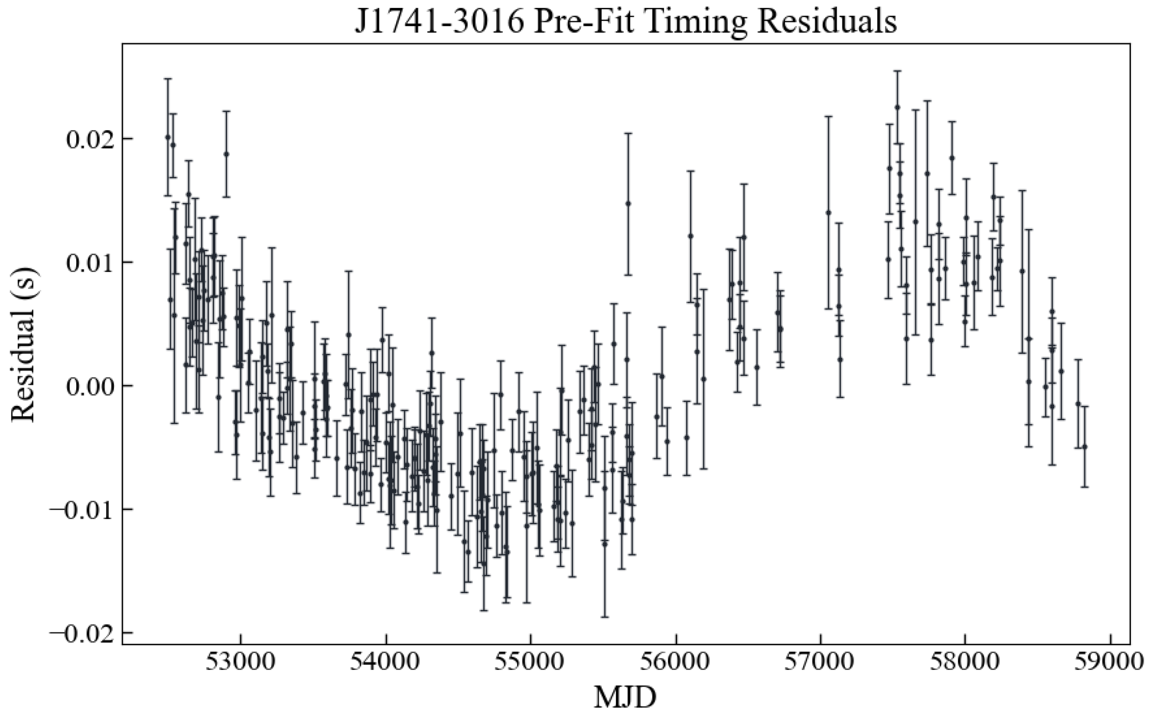
. This table compares the PSRCAT catalog values with our PINT and TEMPONEST results, showing improved positional accuracy (RA uncertainty reduced from 6 ms to 1 ms). The updated spin parameters ($\nu$, $\dot{\nu }$) align with previous studies but with tighter error bounds. The pre-fit residuals for PSR J1741—3016 are shown in Figure 1.

The timing residuals are defined as the differences between the observed pulse arrival times and predictions from the timing model as a function of Modified Julian Date (MJD) (MJD = Julian Date − 2,400,000.5, a continuous count of days primarily used in astronomical timing applications). Figure 1 displays the pre-fit residuals spanning over 17 years, which exhibit two key features: (1) a long-term cubic trend indicating unmodeled spin frequency derivatives and (2) systematic offsets between different observational epochs (vertical groupings). These characteristics fundamentally motivated our subsequent red noise analysis using PINT’s WaveX framework.

3.1. Noise Model

3.1.1. White Noise

White noise refers to noise components that are independent for each TOA and can be modeled as an uncorrelated Gaussian noise process. It is characterized by a scale factor, which is utilized for correlation analysis in the ScaleToaError component module within PINT [26]. Mathematically, white noise is represented by a diagonal matrix N, populated by the scaled TOA variances ${\varsigma }_i^2$:

$$\begin{array}{c}\hfill {\varsigma }_i^2=F_i^2\left({\sigma }_i^2+Q_i^2\right),\end{array}$$

(2)

where

$$\begin{array}{cc}\hfill F_i& =\prod _a{f}_a^{{\mathcal{F}}_{ia}},\hfill \end{array}$$

(3)

$$\begin{array}{cc}\hfill Q_i^2& =\sum _a{q}_a^2{\mathcal{Q}}_{ia}.\hfill \end{array}$$

(4)

where $f_a$ and $q_a$ are referred to as the EFAC (error factor) and EQUAD (error added in quadrature), respectively. Additionally, ${\mathcal{F}}_{ia}$ and ${\mathcal{Q}}_{ia}$ represent TOA selection masks, which can be 0 or 1 based on specific criteria that may depend on the observing epoch, observing frequency, observing system, and other relevant factors.

3.1.2. Red Noise

Red noise is typically associated with long-term irregularities in a pulsar’s rotation, often referred to as spin noise or achromatic red noise (ARN). This type of noise arises from intrinsic pulsar dynamics, such as rotational distortions or irregular changes in spin. The power spectrum of achromatic red noise can be described using a Fourier Gaussian process model [41]:

$$\begin{array}{c}\hfill P\left(f\right)=A_{\mathrm{red}}^2{\left({\displaystyle \frac{f}{f_{\mathrm{yr}}}}\right)}^{{\gamma }_{\mathrm{red}}}\end{array}$$

(5)

where f denotes the frequency component of red noise, $A_{\mathrm{red}}$ is the amplitude of the red noise in μs ${\mathrm{yr}}^{1/2}$, ${\gamma }_{\mathrm{red}}$ is the spectral index, and $f_{\mathrm{yr}}=1{\mathrm{yr}}^{-1}$. This power-law model is implemented in the PLRedNoise component module within PINT.

When fitting red noise, PINT first fits the Fourier series as representation of achromatic red noise (WaveX component) and subsequently estimates the spectral parameters [40].

3.2. Timing Parameters

Table 1 presents the newly obtained timing parameters for PSR J1741—3016 using the aforementioned fitting methods. This includes the updated position and spin parameters. The column labeled “PSRCAT” displays earlier position information and spin parameters obtained from the ATNF Pulsar Catalogue V2.5.1, along with the dispersion measure and Faraday rotation measure for PSR J1741—3016 [33]. The position measurements in this study show a moderate improvement in precision compared to earlier results.

3.3. Timing Noise

3.3.1. White Noise

We characterized the white noise component of PSR J1741—3016 using EFAC and EQUAD parameters, as detailed in Section 3.1.1. The ECORR parameter, which typically accounts for correlated noise sources such as pulse jitter, radio frequency interference (RFI), polarization miscalibration, or interstellar scattering, which are correlated across different frequency sub-bands within the same observation. Since all our observations were conducted at around 1540 MHz, there was no need to include the ECORR parameter.

To evaluate the necessity of including the EFAC and EQUAD in the noise model, we employed the Akaike Information Criterion (AIC) in PINT for model comparison.

AIC, an asymptotically unbiased estimator of the expected Kullback–Leibler (K-L) information, is defined as:

$$\mathrm{AIC}=2q-2ln\widehat{L}$$

(6)

where q represents the total number of free parameters, including those from both the timing model and the noise model. L denotes the maximum likelihood of the model, and $\widehat{L}$ corresponds to the maximum likelihood value at optimal parameters. Among candidate models applied to the same data, the preferred model is the one that minimizes the AIC (with the smallest ${\mathrm{AIC}}_{\min }$) [30]. Individual AIC results are not interpretable as they include arbitrary constants and are significantly influenced by sample size; therefore, we define the difference ${\Delta }_i$:

$${\Delta }_i={\mathrm{AIC}}_i-{\mathrm{AIC}}_{\min }$$

(7)

where ${\mathrm{AIC}}_{\min }$ represents the minimum among the R different ${\mathrm{AIC}}_i$ results (i.e., the minimum occurs at $i=\min$). This transformation ensures that the best-fitting model has $\Delta =0$, while all other models yield positive ${\Delta }_i$. Consequently, a larger ${\Delta }_i$ indicates that the fitted model i is less likely to be the best approximating model within the candidate set.

To evaluate the white noise model, we set up four parameter fitting scenarios: (1) fixed EFAC = 1 and EQUAD = 0; (2) free EFAC with EQUAD = 0; (3) fixed EFAC = 1 with free EQUAD; (4) free EFAC and EQUAD.

Since observations were conducted with two distinct backends—an analog filterbank (AFB) before 2010 and a digital filterbank (DFB) after 2010—we included separate EFAC and EQUAD parameters for each. The Akaike Information Criterion (AIC) was used to select the optimal configuration.

Table 2. AIC differences for different noise model configurations for simulation with EFAC and EQUAD (white noise only).

Parameter Combination	AIC	Difference
EFAC = 1, EQUAD = 0	−1867	311
EFAC = 1, EQUAD free	−2168	10
EFAC free, EQUAD = 0	−2178	0
EFAC free, EQUAD free	−2173	5

presents the AIC results for these scenarios, showing that fitting the EFAC alone provided the best model.

The fitted EFAC values are as follows:

Since our data were obtained using two different backends, an analog filterbank (AFB) before 2010 and a digital filterbank (DFB) after 2010, we included two sets of EFAC and EQUAD parameters for each. The Akaike Information Criterion (AIC) was used to select the optimal configuration. Table 2 presents the AIC results for these scenarios, showing that fitting the EFAC alone provided the best model. Finally, after the fitting process, we obtained EFAC values are as follows: EFAC(FB) (Analog Filterbank backend, pre-2010) = 1.46 ± 0.08 and EFAC(Urum) (Urumqi Digital Filterbank backend, post-2010) = 2.65 ± 0.23.

3.3.2. Red Noise

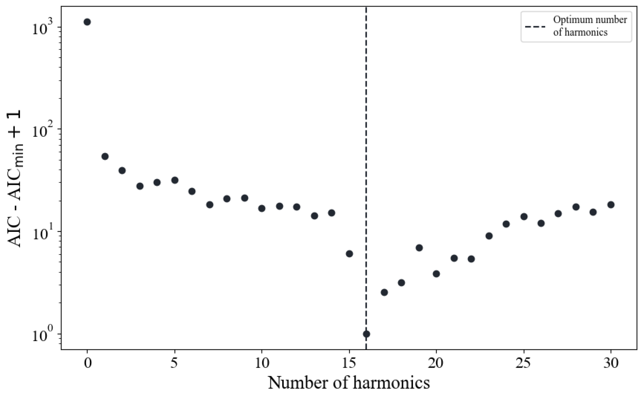
We employed the WaveX model to characterize the noise, as described in Section 3.3.1, utilizing harmonics at frequencies corresponding to the fundamental frequency of the span $T_{\mathrm{span}}^{-1}$, where $T_{\mathrm{span}}$ is the total observation span. To determine the optimal number of harmonics required for modeling the noise, we fitted the TOAs using varying numbers of harmonics and calculated the corresponding AIC for each case. 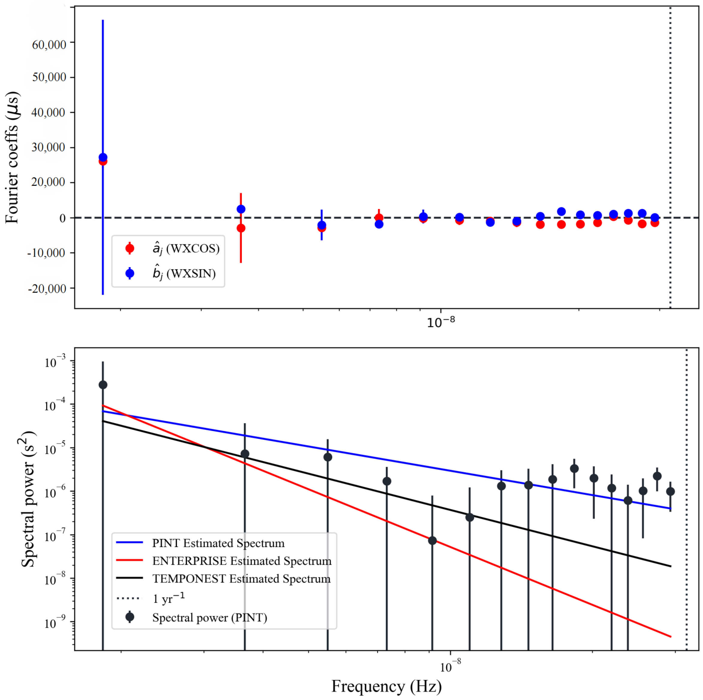Figure 2 illustrates the AIC comparison results, showing that the minimum AIC difference is achieved with 16 harmonics. The upper panel of Figure 3 displays the maximum likelihood estimates of the Fourier coefficients incorporated into the model. A power-law fit was applied to these estimated coefficients, and the lower panel of Figure 3 shows the resulting best-fit power-law model.

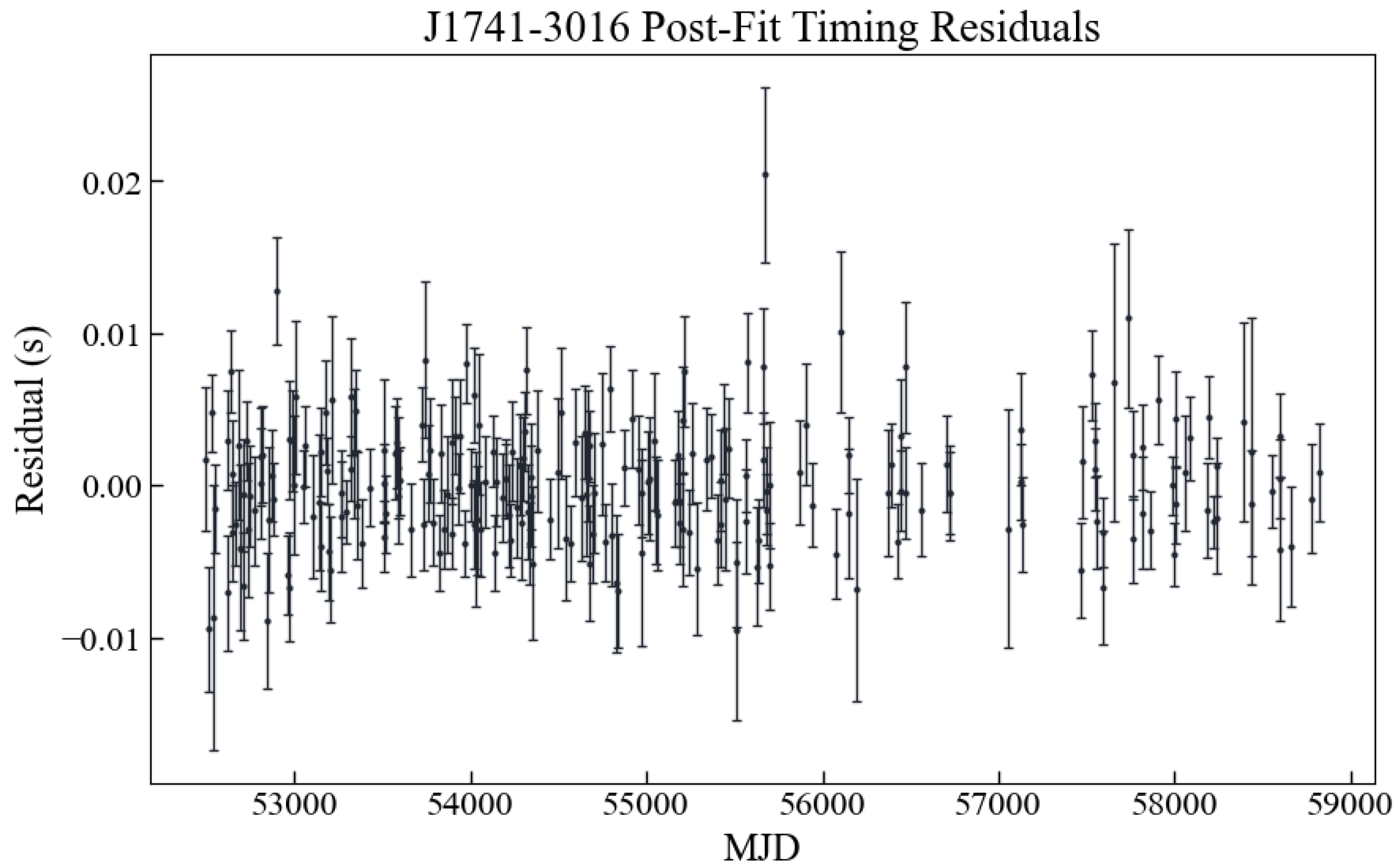
The final fitting results of the red noise parameters are as follows: $\gamma =1.86\pm 0.37$ and ${log}_{10}A=-9.07\pm 0.13$. These results are further compared with Bayesian frameworks in Section 3.4. The residuals after fitting are illustrated in Figure 4, revealing that the model provides a good fit, and almost only Gaussian random components remain.

3.4. Results Comparison

In the preceding sections, we detailed the modeling of timing noise for PSR J1741—3016, including the characterization of white and red noise components. Using the PINT framework, we achieved robust parameter estimation and model selection, with white noise results summarized in Table 2. A detailed comparison of these findings with Bayesian frameworks (TEMPONEST and ENTERPRISE), including implications for red noise characterization, will be presented later in this section.

For TEMPONEST and ENTERPRISE, the prior setting for white and red noise-related parameters from PINT are detailed in

Table 3. Prior ranges on pulsar and timing noise parameters.

Parameter	Symbol [Units]	Prior Range	Prior Type
White noise fitting factor	EFAC	(−1, 2)	Uniform
Red noise amplitude	A [yr3/2]	(−20, $-3$)	log-Uniform
Red noise spectral index	$\gamma$	(0, 20)	Uniform

. Similar prior settings have been widely used in the literature. The absence of multiband observations posed a significant limitation, preventing a robust separation of potential dispersion measure (DM) variations from intrinsic red noise in the timing residuals of PSR J1741—3016. Consequently, advanced methodologies such as DMWaveX, which require high-precision, multi-frequency data to model and characterize DM fluctuations, could not be applied reliably in this analysis. The lack of multiband observations precludes a robust disentanglement of potential dispersion measure (DM) variations from intrinsic red noise in the timing residuals of PSR J1741—3016. As a result, methodologies such as DMWaveX, which require high-precision, multi-frequency data to model and characterize DM fluctuations, could not be applied reliably in this analysis.

It is evident from

Table 4. Timing noise parameter comparison.

Parameter	PINT	ENTERPRISE	TEMPONEST
EFAC (FB)	1.46 ± 0.08	1.27 ± 0.14	1.27 ± 1.06
EFAC (Urum)	2.65 ± 0.23	2.59 ± 0.53	2.58 ± 1.11
$\gamma$	1.86 ± 0.37	4.41± 2.13	3.72 ± 1.21
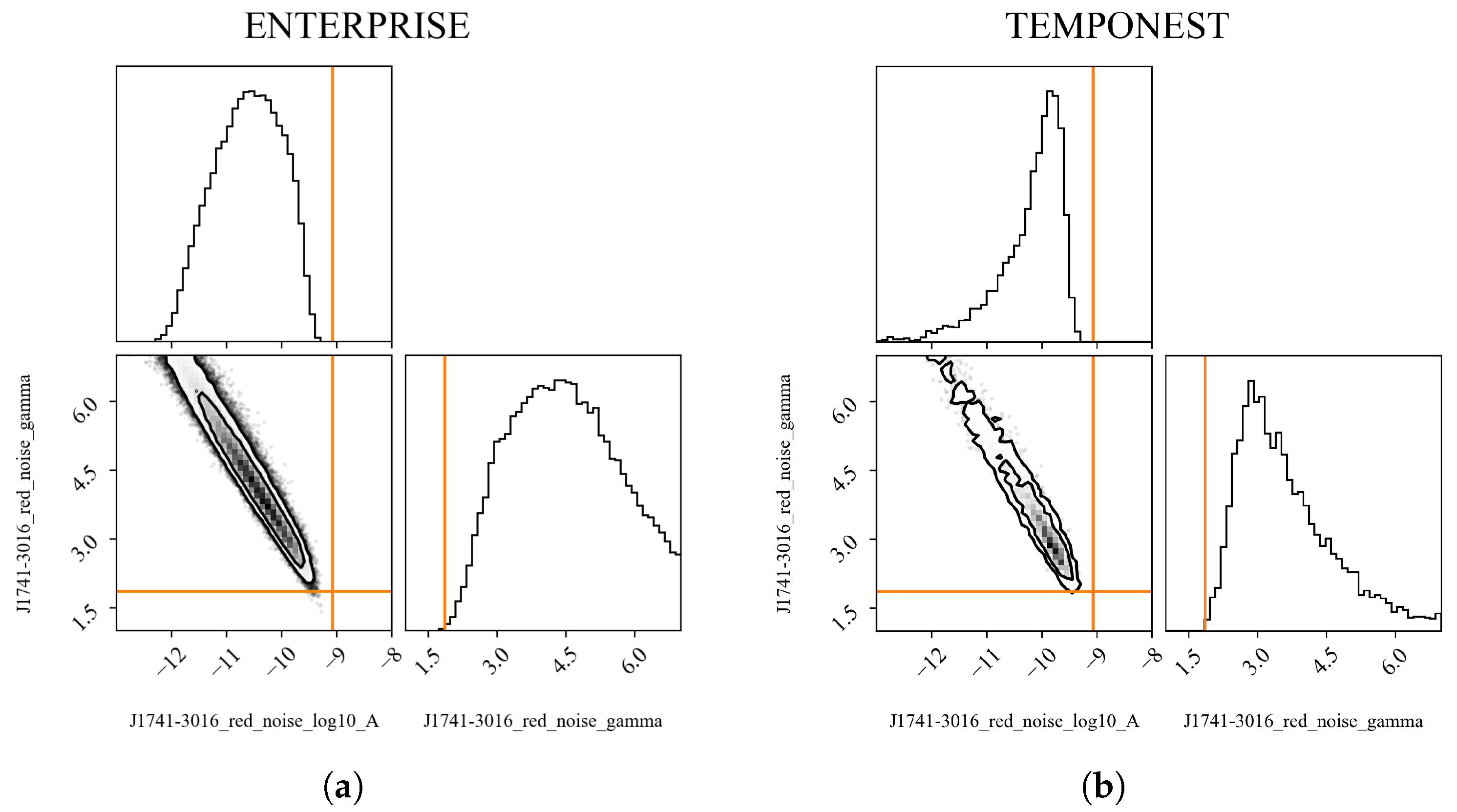
Log10A	−9.07 ± 0.13	−10.59 ± 1.09	−9.75 ± 0.60

that the two methods yield consistent results for the white noise parameters. However, TEMPONEST shows larger uncertainties, as illustrated in the corner plots (Figure 5). Similarly, the results for the red noise parameters are also comparable across methods, though the convergence profile of ENTERPRISE appears to be more dispersed (Figure 6).

When comparing the results of PINT with those obtained using TEMPONEST and ENTERPRISE, we find a slight difference in the EFAC(FB), while the EFAC(Urum) fitting outcomes closely align with those from the other two Bayesian methods. Regarding the red noise fitting, there are minor differences in the fitted $\gamma$, although the fitted results for ${log}_{10}A$ are relatively consistent.

In terms of computational efficiency, PINT demonstrates significant advantages over Bayesian frameworks. As shown in

Table 5. Computational performance comparison. All benchmarks were performed on identical hardware: Dual Intel Xeon 6346 (3.1 GHz, 16C), 1 TB DDR4-3200 RAM, and NVIDIA RTX 3090 GPUs.

Framework	Runtime (s)	CPU Utilization (%)
ENTERPRISE	347.8	26
PINT	165.8	4
TEMPONEST	283.2	34

, PINT(v0.9.8) completes the noise characterization process in 165.8 s with only 4% average CPU utilization, compared to 347.8 s (26% CPU) for ENTERPRISE(v3.4.2) and 283.2 s (34% CPU) for TEMPONEST(v0.1.0). This efficiency gain stems from PINT’s optimized frequentist approach that avoids computationally intensive Bayesian sampling while maintaining comparable accuracy.

4. Discussion and Summary

PSR J1741—3016 is a young radio pulsar with a characteristic age of $3.34\times {10}^5$ years. This study presented a comprehensive timing analysis of PSR J1741—3016, based on 17.5 years of observational data collected with the Nanshan 25 m radio telescope. Using the PINT framework, we modeled the pulsar’s spin parameters, position, and timing noise, including both white noise and red noise components. The Akaike Information Criterion (AIC) was applied to evaluate various noise models and parameter configurations, achieving an optimal balance between model complexity and goodness of fit. This highlights PINT’s capability to handle datasets effectively while maintaining accurate noise characterization.

The red noise modeling process also revealed differences in the number of Fourier coefficients employed by each framework: PINT required 16 coefficients, TEMPONEST utilized 52, and ENTERPRISE applied the default 30 coefficients. These variations reflect differing approaches to noise modeling, with PINT striking a balance between computational efficiency and model complexity. This highlights PINT’s capability to handle large datasets effectively while maintaining accurate noise characterization.

One notable outcome of this analysis is the overall consistency of the timing solutions obtained using PINT, TEMPONEST, and ENTERPRISE. While minor differences were observed in specific parameters, particularly the red noise spectral indices, the general agreement among these methods underscores the robustness of the frameworks. Notably, these models demonstrated exceptional efficiency, delivering comparable results in significantly shorter computation times, making them practical tools for timing studies of young pulsars.

The advanced visualization tools in PINT, including Fourier coefficient plots, power spectrum estimates, power-law fits, and post-fit residuals further illustrate its strengths. These features enabled us to assess the appropriateness and reasonableness of the red noise model. For the red noise parameters, we obtain ${log}_{10}{A}_{\mathrm{red}}=-9.07\pm 0.13$ and $\gamma =1.86\pm 0.37$. Furthermore, our results are consistent with the conclusion that the strength of timing noise scales proportionally to ${\nu }^1{\left|\dot{\nu }\right|}^{-0.6\pm 0.1}$ [18], where $\nu$ is the pulsar’s spin frequency and $\dot{\nu }$ is its spin-down rate. To account for changes in the observational backend systems, we separately modeled the white noise parameters EFAC and EQUAD for data collected before and after 2010. The final residuals, dominated by Gaussian random noise, demonstrate that the noise model was effectively characterized.

This analysis of PSR J1741—3016 not only demonstrates the capability of PINT to handle time noise in young pulsars but also highlights its potential for study timing noise in large pulsar samples. This will enable a more comprehensive understanding of timing irregularities and their physical origins. Multi-frequency observations and longer time spans will be essential for disentangling contributions from dispersion measure variations and intrinsic red noise.

The computational efficiency metrics in Table 5 demonstrate PINT’s practical advantages for long-term timing studies. The 60% reduction in runtime compared to TEMPONEST, combined with significantly lower CPU utilization (4% vs. 34%), makes PINT particularly suitable for analyzing large pulsar populations or performing iterative model refinement. These benchmarks were conducted on enterprise-grade hardware (see Table 5) to ensure method reproducibility. Notably, the performance advantage persists even when utilizing high-performance computing resources, as PINT’s algorithm design minimizes both computational complexity and memory footprint.