A Dynamic Shortest Travel Time Path Planning Algorithm with an Overtaking Function Based on VANET

Abstract

With the rapid development of the economy, urban road congestion has become more serious. The travel times for vehicles are becoming more uncontrollable, making it challenging to reach destinations on time. In order to find an optimal route and arrive at the destination with the shortest travel time, this paper proposes a dynamic shortest travel time path planning algorithm with an overtaking function (DSTTPP-OF) based on a vehicular ad hoc network (VANET) environment. Considering the uncertainty of driving vehicles, the target vehicle (vehicle for special tasks) is influenced by surrounding vehicles, leading to possible deadlock or congestion situations that extend travel time. Therefore, overtaking planning should be conducted through V2V communication, enabling surrounding vehicles to coordinate with the target vehicle to avoid deadlock and congestion through lane changing and overtaking. In the proposed DSTTPP-OF, vehicles may queue up at intersections, so we take into account the impact of traffic signals. We classify road segments into congested and non-congested sections, calculating travel times for each section separately. Subsequently, in front of each intersection, the improved Dijkstra algorithm is employed to find the shortest travel time path to the destination, and the overtaking function is used to prevent the target vehicle from entering a deadlocked state. The real-time traffic data essential for dynamic path planning were collected through a VANET of symmetrically deployed roadside units (RSUs) along the roadway. Finally, simulations were conducted using the SUMO simulator. Under different traffic flows, the proposed DSTTPP-OF demonstrates good performance; the target vehicle can travel smoothly without significant interruptions and experiences the fewest stops, thanks to the proposed algorithm. Compared to the shortest distance path planning (SDPP) algorithm, the travel time is reduced by approximately 36.9%, and the waiting time is reduced by about 83.2%. Compared to the dynamic minimum time path planning (DMTPP) algorithm, the travel time is reduced by around 18.2%, and the waiting time is reduced by approximately 65.6%.

1. Introduction

With the rapid development of the global economy and the continuous acceleration of urbanization, the number of cars has explosively increased. As of 2023, the number of private cars in China has reached 294 million [1]. though private cars provide convenience in daily life, they also bring unprecedented challenges to road traffic, such as frequent traffic congestion, frequent traffic accidents, fuel wastage, and pollution. All of these issues have severely restricted the development of cities. With the continuous improvement of Internet of Things technology, the interconnection of people, vehicles, and infrastructure has gradually become a reality. This provides us with a feasible way to solve the above problems through the intelligent transportation system (ITS). In ITS, route planning is one of the focal points of attention. Its primary objective is to find an optimal path within a given travel time [2], assisting vehicles in reaching their destination safely and quickly.

Vehicular ad hoc networks (VANETs) provide possible ways to realize ITS. The VANET architecture is based on vehicle-to-vehicle (V2V), vehicle-to-infrastructure (V2I), and infrastructure-to-infrastructure (V2I) communication systems for data exchange between on-board units (OBUs) and roadside units (RSUs) [3], as shown in Figure 1. Road traffic-related data, such as speed, travel destination, and distances among vehicles, can be obtained via GPS and exchanged among vehicles and RSUs by wireless communication links, as seen in Figure 1. The main applications of VANET can be divided into three categories [4]: (1) Road safety applications, where VANET can help prevent accidents on the road and identify stationary or moving obstacles. (2) Traffic optimization and driver assistance applications, where VANET enables the collection and sharing of vehicle data, which can be used to improve traffic conditions. (3) Information and entertainment, where VANET can provide in-vehicle entertainment and information services to enhance the driving experience for drivers and passengers. Thus, in the VANET environment, autonomous vehicles can share information and interact with other vehicles and road equipment through OBU to achieve safer and more efficient autonomous driving.

Figure 1. A VANET scenario.

However, due to various uncertain factors, such as road construction, adverse weather conditions, traffic accidents, and congestion, vehicles designated for special emergency tasks (e.g., private cars transporting pregnant women and children for medical treatment, and emergency transport vehicles) may not reach their destination within an ideal time. Given the randomness and uncertainty of the traffic conditions on the road, vehicles can encounter congested road segments and can also be surrounded by slower vehicles, leading to extended travel times. To avoid wasting time on the road, we propose a VANET-based dynamic shortest travel time path planning algorithm with an overtaking function (DSTTPP-OF). The proposed DSTTPP-OF aims to bypass congested road segments quickly and avoid blocking by surrounding slower vehicles.

The purpose of this article is to enable the target vehicle to reach the specified destination in the shortest travel time. The proposed DSTTPP-OF consists of the following two functions:

• Path planning: At a certain distance before each intersection, the onboard unit obtains information about the speed and position of vehicles on each road segment through V2I and V2V communication. We estimate the travel time for each segment and calculate the shortest time path to the destination using the improved Dijkstra algorithm. This path is then used as the driving route for the target vehicle.
• Overtaking planning: Within a certain range on each road segment, when the target vehicle is surrounded by slower vehicles, the V2V communication is used to transmit speed change information to the slower vehicles, creating enough space for the high-speed vehicle to change lanes and overtake.

This article is organized as follows. In Section 1, we provide a brief introduction to the proposed scheme. In Section 2, we analyze recent related work and summarize the contributions of this paper. In Section 3, we propose a dynamic shortest-path algorithm with an overtaking function. In Section 4, experimental simulations are presented for the analysis of the proposed algorithm. In Section 5, we provide a summary of this paper.

2. Related Work

Route planning is a classic shortest-path problem. The optimal route from the source to the destination is based on certain criteria, often involving metrics such as driving distance (shortest route) [5], travel time (fastest route) [6,7], energy consumption (most economical route) [8,9], or a combination of these factors [10]. The most well-known solution for route planning is the Dijkstra algorithm [11]. With economic development and the accelerated urbanization process, traffic congestion has become a more serious problem [12]. When planning vehicle travel paths, congested road segments are not avoided. This is because the shortest-path planning based on distance may pass through congested road segments; changes in traffic conditions may cause certain segments to become congested, resulting in significant travel time wastage. The same holds true for shortest-path planning based on static time considerations [13]. For drivers, obtaining real-time traffic information and planning a reasonable route are the most effective methods to avoid traffic congestion.

Scholars have conducted extensive research on path planning to obtain the optimal path. Cao et al. [2] proposed a data-driven approach. They transformed the original shortest-path problem into a cardinality minimization problem based on travel time samples on each road, using 1-norm minimization techniques and variants to solve the cardinality minimization problem. Yu et al. [7] designed an automatic valet parking route planning scheme that enables vehicles to reach parking spaces in the shortest time. They considered some dynamic factors in valet parking lots based on the Dijkstra algorithm. Typaldos et al. [8] employed a dynamic model of vehicle kinematics, using acceleration as a control variable to address path planning problems. Within a fixed or flexible time range, they optimized the vehicle’s trajectory to maximize the reduction in fuel consumption. Schoenberg et al. [11] proposed an adaptive charging and routing strategy that took into account travel time, waiting time, and charging time. This strategy aims to minimize the waiting times at charging stations and the overall travel times for electric vehicles by informing the central charging station database (CSDB) about the planned charging stations during their journeys. Li et al. [12], looking at factors like travel time, road roughness, road unevenness, and intersections, established a comfort indicator. They designed a cloud-assisted comfort route planning method based on the Dijkstra algorithm. Zhi et al. [13] proposed a dynamic travel time prediction method that transforms the predicted dynamic travel time into the reliability of the travel time. Using this reliability to weight road segments, they applied the Dijkstra algorithm with logarithmic transformations to solve the most reliable path.

However, all of the above route planning solutions primarily focus on minimizing distance, travel time, or energy consumption, and do not consider unexpected events on the roads. It is easy to understand that vehicles may encounter blockages, so a pre-planned route may become obstructed due to road congestion, leading to the vehicle’s path not being dynamically adjusted. Thus, the impacts caused by unexpected events should be considered for path planning.

To address unexpected events on roads, Guo et al. [6] proposed a distributed system architecture for collecting and sharing real-time traffic information, aimed at avoiding congestion and enabling real-time path planning. Peng et al. [14] introduced a multi-route dynamic programming (DP) model that not only identifies the shortest time travel route but also provides multiple comparable optimal routes for vehicles. This allows traffic flow to be distributed across different routes, thereby alleviating congestion. Chavhan et al. [15] designed an efficient, scenario-sensitive vehicle accident route service management system. This system acquires real-time information on events, vehicles, weather conditions, roadside units, and roads, and then shares this information with nearby vehicles and roadside units to provide commuters with the best routes. Refs. [16,17] also employed rerouting systems to avoid traffic congestion, simultaneously reducing travel time, fuel consumption, and carbon dioxide emissions. Oubbati et al. [18] proposed an SDN-based route planning scheme called SEARCH, which dynamically adjusts the optimal path for vehicles during their journeys to avoid congested and blocked roads. It utilizes a macroscopic model to calculate travel times for each road segment and employs the Dijkstra algorithm to find shorter time paths to the destination.

However, Refs. [13,14,15,18] did not account for the impact of traffic signals when calculating travel times on congested roads.

In addition, the impacts of obstacles should also be considered in path planning. Lin et al. [19] proposed an improved A-star algorithm to achieve high efficiency and accuracy for path planning on post-disaster field roads. The algorithm introduces redundant safety spaces to filter out impassable narrow roads and is able to avoid collisions between vehicles and obstacles. Zhou et al. [20] proposed an improved traditional rapid exploring random tree (RRT) obstacle avoidance path planning algorithm based on vehicle kinematic constraints, which is able to generate safe and time-efficient paths in static obstacle environments. Jin et al. [21] presented a novel deep reinforcement learning-based (DRLB)-assisted path planning algorithm for autonomous driving vehicles with a novel deep reinforcement learning framework. At the same time, the artificial potential field approach (APFA) introduced in the algorithm effectively guides the vehicle to move along the predetermined path to the target point, while cleverly avoiding obstacles along the way. Qi et al. [22] proposed a path planning and control framework for autonomous vehicles with low-cost positioning, which is based on reinforcement learning and artificial potential field methods to effectively avoid static and dynamic obstacles.

The above methods effectively avoid obstacles, but they ignore the fact that obstacles often consist of moving vehicles on urban roads. Overtaking path planning is an important part of realizing intelligent driving. Researchers have conducted extensive research on autonomous vehicle overtaking path planning and have proposed a variety of approaches [23].

Meanwhile, most route planning schemes do not consider the influence of surrounding vehicles on the target vehicle. When the target vehicle is surrounded by slower vehicles, it may be stuck in a deadlock that cannot be resolved by overtaking, leading to increased travel times. When vehicles are in a dead-locked state, the vehicles following behind have to wait to pass, resulting in traffic congestion. Moreover, some lanes may be blocked or in closure states; these congested roads and blocked lanes should be avoided when planning the route. Thus, lane changing and overtaking become necessary components of route planning to solve blocked and congested lanes. Considering this, this paper proposes a VANET-based dynamic shortest-path planning method with an overtaking function (DSTTPP-OF). It prevents the target vehicle from entering a deadlock state and enables it to reach its destination more quickly. The main contributions of this paper are as follows:

• As far as we know, few studies take into account the target vehicle becoming stuck in a deadlock caused by surrounding vehicles, especially by the rear vehicles in the adjacent lane during a lane change. Escaping from deadlocked states can cause significant travel delays, so we propose an overtaking algorithm to ensure that the target vehicle travels with the shortest possible travel time and avoids becoming stuck in deadlocked states. We use V2V communication to negotiate with other vehicles, allowing low-speed vehicles to provide enough distance for the target vehicle to execute lane changes and overtaking maneuvers.
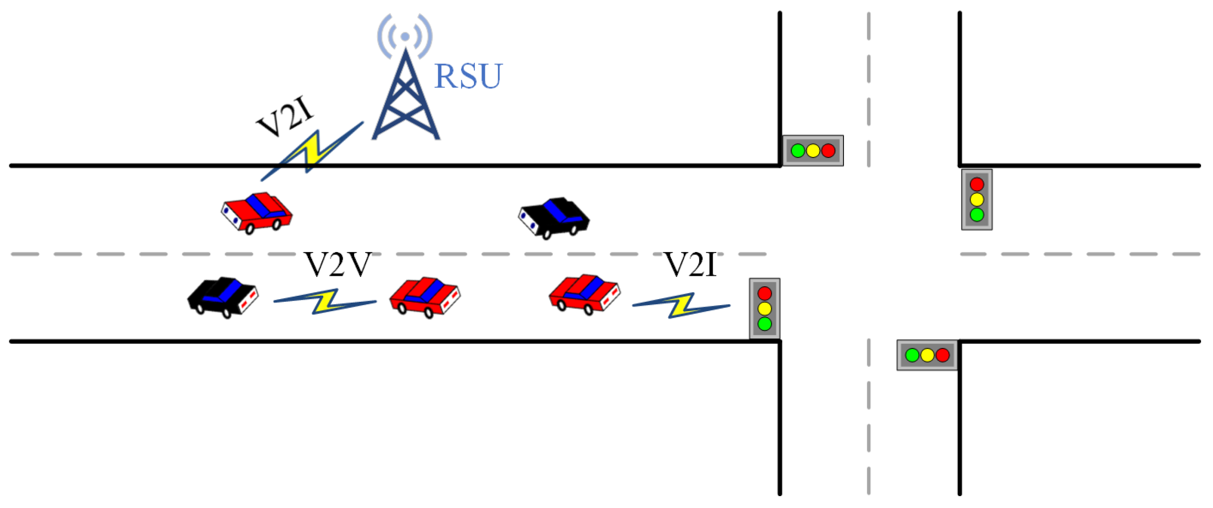
• We assume that the speed and position information of each vehicle on the road can be obtained through V2I and V2V communications in VANET [24,25,26,27]. Based on the real-time road traffic information, we categorize each road segment around the intersection into congested and non-congested segments. So, the estimation of travel time includes the time spent in both congested and non-congested segments, respectively. We provide a detailed method for estimating the travel time for each road segment and then derive the total travel time for the target vehicle.
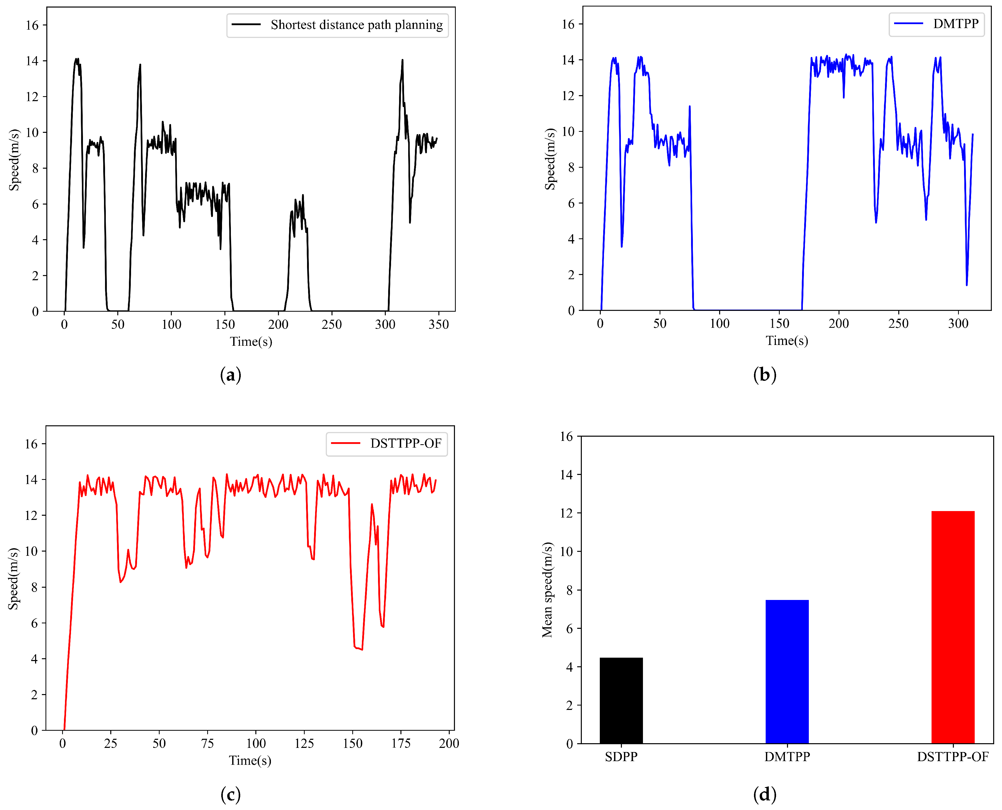
• Considering the influence of surrounding vehicles, we propose a dynamic shortest travel time path planning algorithm with an overtaking function (DSTTPP-OF). The onboard terminal of the target vehicle obtains estimated travel times for each road segment and, prior to reaching each intersection, employs the Dijkstra algorithm to compute shorter travel time routes to the destination. The proposed DSTTPP-OF performs much better than the other algorithms, ensuring that the target vehicle arrives at its destination in the shortest possible time through a smoother driving journey.

3. Dynamic Shortest Travel Time Path Planning Algorithm with an Overtaking Function

In the proposed scheme, we make two assumptions: first, that the impact of pedestrians and non-motor vehicles is not considered, and second, VANET provides high-quality communication, regardless of latency and data loss [28,29]. For the first assumption, in realistic scenarios, non-motor vehicles travel in non-motorized lanes, while motor vehicles use the motor lanes. Typically, non-motorized lanes are segregated from motor lanes, allowing us to consider them as not interfering with each other. Furthermore, pedestrian crossings are primarily located at intersections and are absent within the lane sections. Consequently, pedestrians are not considered as influencing factors in our path planning design. For the second assumption, in the VANET, V2I, V2V, and I2I communications are symmetrically utilized to obtain speed and position information for vehicles on each road, so all the real-time road conditions can be obtained based on the VANET [24,25,26,27], as shown in Figure 2. The wireless network failure is not considered and we assume that wireless communication is always available for exchanging and sharing road traffic conditions. This ensures that speed and position information can be used to calculate the lengths of congested segments and estimate the travel time of each road. Then, both the shortest travel time path planning and the overtaking planning are designed to operate within such a VANET environment.

Figure 2. VANET-based traffic information transmission.

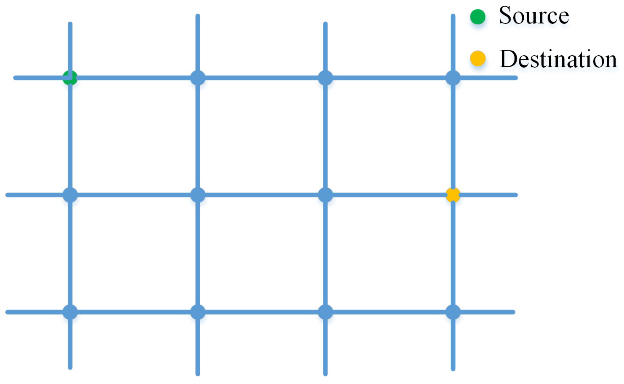
3.1. Road Network Model

The road network is modeled as a directed graph represented by G.

$$G=\left(N,E\right)$$

(1)

where N is the set of road intersections, $N=\{n_1,n_2,\dots ,n_n\}$. E is the set of edges, $E=\{e_{ij}=(n_i,n_j)|n_i,n_j\in N\}$, $e_{ij}$ represents the path that a vehicle takes to begin its journey from the source point $n_i$ to its destination point $n_j$. We define the weight $\omega =(e_{ij},t_{ij})$, where $t_{ij}$ is the average travel time of the path $e_{ij}$, and $\omega >0$. Assigning a time cost weight $\omega$ to each edge transforms the directed graph G into a weighted graph. It is important to note that $t_{ij}$ denotes the average travel time for a vehicle to pass through two intersection roads, $t_{ij}=L_{ij}/v_{ij}$, where $L_{ij}$ is the length of path $e_{ij}$, and $v_{ij}$ is the average travel speed on the road, so the value of $t_{ij}$ is not fixed.

3.2. Estimation of Travel Time

Vehicles inevitably experience queuing at intersections due to traffic signals. According to traffic wave theory [30], the travel segment can be divided into congested segments and non-congested segments around the intersection, denoted as $L_C$ and $L_{NC}$ respectively. ${\rho }_C$ and ${\rho }_{NC}$ is the traffic flow density in these two adjacent different regions, while $v_C$ and $v_{NC}$ is the average traffic speed in these two adjacent different regions, as illustrated in Figure 3.

Figure 3. Two different road regions around the intersection.

According to the Greenshields velocity–density relationship model [31], the speed v can be described as follows:

$$v=v_f(1-\frac{\rho }{{\rho }_{max}})$$

(2)

where $v_f$ denotes the free-flow speed, and $\rho$ denotes traffic flow density, and ${\rho }_{max}$ denotes congestion density.

The average travel time of vehicles can be divided into two parts: the average travel time on congested segments $T_C$ and the average travel time on non-congested segments $T_{NC}$. Thus, the average travel time T is as follows:

$$T=T_C+T_{NC}$$

(3)

From (2), it can be determined that the average travel speed on non-congested segments $v_{NC}$ is as follows:

$$v_{NC}=v_f(1-\frac{{\rho }_{NC}}{{\rho }_{max}})$$

(4)

where ${\rho }_{NC}$ is the traffic flow density on non-congested segments, ${\rho }_{max}=1/\phantom{1\left(l+\delta \right)}\left(l+\delta \right)$, l is the vehicle length, $\delta$ is the minimum safety distance.

Therefore, the average travel time on the non-congested segments $T_{NC}$ is as follows:

$$T_{NC}=\frac{L_{NC}}{v_{NC}}=\frac{L-L_C}{v_f[1-\left({\rho }_{NC}/{\rho }_{max}\right)]}$$

(5)

The average travel time on the congested segments, $T_C$, can be obtained from the vehicle’s length, l, minimum safety distance, $\delta$, between vehicles, and the number of outflow vehicles, $N_{out}$, at the intersection during the green signal period.

$$T_C=\frac{N_q}{N_{out}}=\frac{L_C/(l+\delta )}{N_{out}},N_q\le N_{out}$$

(6)

where $N_q$ is the number of vehicles in the queue waiting around the intersection. When $N_q\ge N_{out}$, vehicles cannot pass through the intersection within the current green signal duration. After waiting for $k(k\in \{0,1,\dots ,n\left\}\right)$ signal cycles, when $N_q<N_{out}$, vehicles can pass through the intersection, as shown in Figure 4.

Figure 4. Traffic conditions at the intersection.

At this point, the average travel time for the congested segment is as follows:

$$T_C=k{t}_{total}+\frac{L_C}{\left(l+\sigma \right)N_{out}},k\in \left\{0,1,2,\dots ,n\right\}$$

(7)

where $T_{total}$ denotes the waiting time for one traffic signal cycle, $T_{total}=T_r+T_g+T_y$, $T_r$ denotes the red signal duration time, $T_g$ denotes the duration time of the green signal, and $T_y$ denotes the duration time of the yellow signal. Derived from (3), (5), (6), and (7), the average travel time, T, for vehicles on road segments, L, is as follows:

$$\begin{array}{cc}\hfill T& =\frac{L-L_C}{v_f[1-\left({\rho }_{NC}/{\rho }_{max}\right)]}+k{T}_{total}+\frac{L_C/(l+\delta )}{N_{out}},\hfill \\ \hfill k& \in \{0,1,\dots ,n\}\hfill \end{array}$$

(8)

3.3. Dynamic Shortest Travel Time Path Planning with an Overtaking Function

In this section, the proposed dynamic shortest travel time path planning algorithm with an overtaking function (DSTTPP-OF) based on VANET is presented. It comprises dynamic shortest travel time path planning, real-time vehicle detection, and overtaking planning. This proposed algorithm follows the steps below:

Step 1: Utilizing the improved Dijkstra algorithm based on the estimated travel time for each road segment, calculate the shortest travel time route to the destination. Update the target vehicle’s shortest travel time path at a certain longer distance threshold $\eta$ before each intersection.

Step 2: Continuously monitor the surrounding conditions of the target vehicle in real time, recording the IDs of the front vehicle, adjacent front vehicle, and adjacent rear vehicle.

Step 3: When the distance between the vehicle and the intersection is greater than $\eta$—if the distance between the target vehicle and the front vehicle is less than the shorter distance threshold $\alpha$, initiate overtaking planning based on the IDs of the adjacent front and rear vehicles. If there are no adjacent front or rear vehicles, the target vehicle can change lanes directly. If they exist, calculate the distance between the target vehicle and the front or rear vehicle in the adjacent lane. Then, based on these distances, determine whether the target vehicle can change lanes directly or if the front or rear vehicle in the adjacent lane needs to decelerate to provide sufficient space for the target vehicle to overtake. The distance thresholds can be set as needed; in this paper, we set the longer threshold, $\eta$, to 120 m and the shorter threshold, $\alpha$, to 30 m.

In the traditional path planning algorithm, when a vehicle requests to reach its destination, the control center using a centralized architecture attempts to calculate a complete path based on features such as distance and travel time. But they do not consider some possible unexpected events that may result in traffic congestion [18]. Therefore, our proposed DSTTPP-OF attempts to consider the traffic congestion issue and aims to avoid traffic congestion and accidents by calculating the shortest travel time path.

Calculate the average travel time for each road segment using (8), and establish the adjacency matrix B based on the directed weighted graph G.

$$B=\left(\begin{array}{cccc}{T}_{00}& T_{01}& \cdots & T_{0n}\\ T_{10}& T_{11}& \cdots & T_{1n}\\ ⋮& ⋮& \ddots & ⋮\\ T_{n0}& T_{n1}& \cdots & T_{nn}\end{array}\right)$$

(9)

Then, calculate the shortest travel time path using the improved Dijkstra algorithm:

Step 1: Initialize the set S, $dist\left[\right]$, $path\left[\right]$.

$$\begin{array}{}\hfill \mathrm{(10)}& \hfill S& =& \left\{n_0\right\}\hfill \hfill \mathrm{(11)}& \hfill dist\left[i\right]& =& T_{0i}\hfill \hfill \mathrm{(12)}& \hfill path\left[i\right]& =& -1\hfill \end{array}$$

where $n_0$ is the source point, S is the set of vertices on the shortest path, $dist\left[i\right]$ is the travel time from $n_0$ to $n_i$ when ($n_0$ is adjacent to $n_i$). If $n_0$ and $n_i$ are not adjacent, the travel time is ∞, and $path\left[i\right]$ is the predecessor node of the shortest travel time from the source point to the point $n_i$.

Step 2: Select the point $n_j$ with the shortest travel time from the set of vertices, $N-S$.

$$\begin{array}{cc}\hfill S& =S\cup \left\{n_j\right\},\hfill \\ \hfill dist\left[j\right]& =\min \{\left.dist\left[i\right]\right|n_i\in N-S\}\hfill \end{array}$$

(13)

Step 3: Update the shortest travel time from vertex $n_0$ to any vertex $n_k$ in the set $N-S$.

$$\begin{array}{}\hfill \mathrm{(14)}& \hfill dist\left[k\right]& <& dist\left[j\right]+T_{jk}\hfill \hfill \mathrm{(15)}& \hfill dist\left[k\right]& =& dist\left[j\right]+T_{jk}\hfill \hfill \mathrm{(16)}& \hfill path\left[k\right]& =& j\hfill \end{array}$$

Step 4: Repeat the operations of Step 2 and Step 3 a total of $n-1$ times until all vertices are included in the set S.

Figure 5a illustrates the traffic road network we have established. In Figure 5, the red vehicle is planning to travel from $n_1$ to $n_8$. It will obtain real-time travel time for each road segment and utilize the Dijkstra algorithm to dynamically calculate the shortest travel time path in advance based on collected real-time road information by V2V and V2I communications. At a distance of $\eta =120$ meters before arriving at each intersection, the red vehicle’s travel path is updated according to the calculated results. The red vehicle (target car) is located on the edge, $e_{15}$, with its destination at $n_8$. The original travel path of the red vehicle is $e_{15}\to e_{56}\to e_{67}\to e_{78}(n_1\to n_5\to n_6\to n_7\to n_8)$, without considering any congestion, as shown in Figure 5b. However, this travel path may not last for a long time due to traffic congestion occurring in $e_{67}$, so the original path may no longer be the shortest travel time path. Thus, it is necessary to consider the current intersection $n_6$ as the starting point and restart path planning to choose a new path. The update path planning result (shortest travel time path) is $e_{610}\to e_{1011}\to e_{1112}\to e_{128}$$(n_6\to n_{10}\to n_{11}\to n_{12}\to n_8)$, as shown in Figure 5c. Due to traffic congestion occurring again on route $e_{1112}$, the shortest time path changes. Therefore, the travel route is re-planned, starting from the point $n_{11}$. This segment of the path commenced from the intersection $n_{11}$, reaching the destination $n_8$ through the path $e_{117}\to e_{78}$$(n_{11}\to n_7\to n_8)$, as presented in Figure 5d for details.

Figure 5. Dynamic shortest travel time route: (a) Traffic road network. (b) Original travel path. (c) Traffic congestion occurred in $e_{67}$ and re-planned a new path from point $n_6$. (d) Traffic congestion occurred in $e_{1112}$ and re-planned a new path from point $n_{11}$.

We converted the road network in Figure 5 into a directed weighted graph composed of nodes and edges, setting the travel time for each path as the weight; the weighted graph is shown in Figure 6. Each edge requires a maximum of 40 s of travel time under normal traffic conditions. The travel time for each edge depends on the real-time traffic conditions along the route. Throughout the journey, the itinerary of the red vehicle changed twice at intersections $n_6$ and $n_{11}$, to avoid congested segments $e_{67}$ and $e_{1112}$. Initially, the computed route for the red vehicle was $n_1\to n_5\to n_6\to n_7\to n_8$, with an estimated travel time of 170 s. When congestion occurred on path $e_{67}$, the algorithm lets the vehicle change to another road with the shortest time. The shortest time path was $n_6\to n_{10}\to n_{11}\to n_{12}\to n_8$, with an estimated time of 180 s for this segment. When the red vehicle was driving on section $e_{1112}$, it found that the section ahead was congested, so the path changed again, and the new shortest time path was $n_{11}\to n_7\to n_8$, estimated to arrive at the destination in 95 s. Finally, the red vehicle reached its destination after 265 s. Algorithm 1 illustrates the entire process, and Table 1 summarizes this process and provides the estimated travel time for each route, as presented in Figure 6.

Algorithm 1 Dynamic shortest travel time route based on the improved Dijkstra

Input: $T_{car}$: Target vehicle’s ID $E=\left[e_{ij}\right]$    //A set of edge. $N=\left[n_i\right]$    //A set of intersections. for $e_{ij}$ in $E$ do       Calculate $T_{ij}$    //The average travel time of $e_{ij}$. $G=(N,\mathbf{B})$ for $n_i$ in $N$ do        $\mathrm{STR}=\mathrm{Dijkstra}(G,n_i,n_j)$   //The shortest travel time route ($n_i$ is the origin, $n_j$ is the destination).        if $\kappa \le \mathrm{position}\left(n_i\right)-\mathrm{position}(T_{car})\le \eta$ then              Set $\mathrm{route}(T_{car},\mathrm{STR})$      else end

Figure 6. The weighted graph of Figure 5: (a) is the weighted graph of Figure 5b; (b) is the weighted graph of Figure 5c; (c) is the weighted graph of Figure 5d.

Table 1. Driving path and time.

Source	Destination	Driving Path	Travel Time	Update Route
$n_1$	$n_8$	$n_1\to n_5\to n_6\to n_7\to n_8$	170 s	$n_6$
$n_6$	$n_8$	$n_6\to n_{10}\to n_{11}\to n_{12}\to n_8$	180 s	$n_{11}$
$n_{11}$	$n_8$	$n_{11}\to n_7\to n_8$	95 s	none
$n_1$	$n_8$	The full path: $n_1\to n_5\to n_6\to n_{10}\to n_{11}\to n_7\to n_8$	Total travel time: 265 s

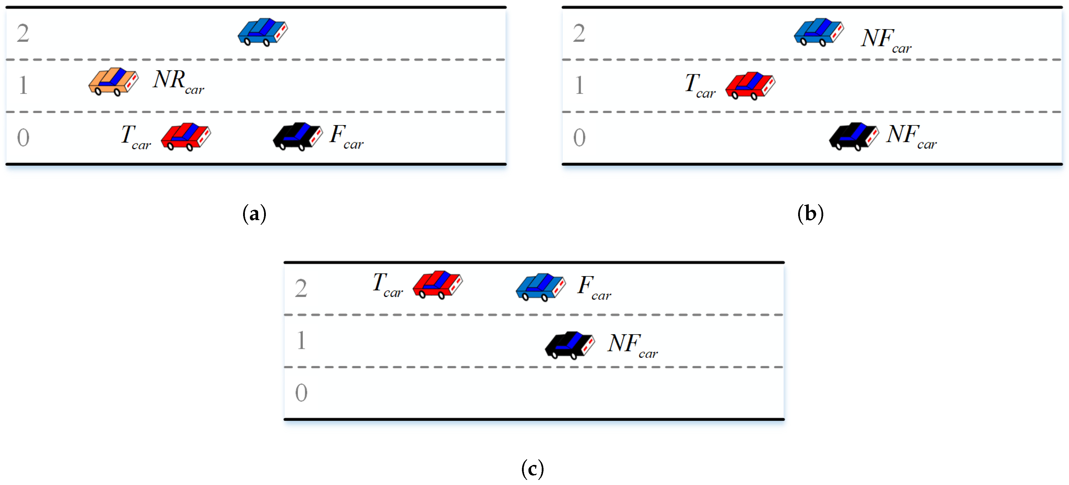
3.4. Overtaking Planning

During the driving process, the target vehicle needs to continuously detect surrounding vehicles in real time and obtain their IDs. After obtaining these IDs, the conditions of the target vehicle in proximity can be understood, and overtaking maneuvers can be planned for the shortest travel time. $F_{car}^{ID}$ is used to store the ID of the vehicle in front of the target vehicle, $N{F}_{car}^{ID}$ is used to store the ID of the front vehicle in the adjacent lane, and $N{R}_{car}^{ID}$ is used to store the ID of the rear vehicle in the adjacent lane.

In Figure 7, the target vehicle is the red car, and each road has three lanes. In Figure 7a, the red vehicle has a black vehicle as its front car; there is no front car in the adjacent lane, but there is a rear car in the adjacent lane. Therefore, $F_{car}^{ID}$ is the ID of the black vehicle, $N{F}_{car}^{ID}$ is empty, and $N{R}_{car}^{ID}$ is the ID of the orange vehicle. In Figure 7b, the red vehicle has no front car, but both adjacent lanes have front cars and no rear cars. So, in this case, $F_{car}^{ID}$ is empty, $N{F}_{car}^{ID}$ denotes the IDs of the black vehicle and blue vehicle, and $N{R}_{car}^{ID}$ is empty. In Figure 7c, the red vehicle has a blue vehicle as its front car, and the adjacent lane has a front black car, but no rear car. Clearly, in this case, $F_{car}^{ID}$ is the ID of the blue vehicle, $N{F}_{car}^{ID}$ is the ID of the black vehicle, and $N{R}_{car}^{ID}$ is empty. Algorithm 2 illustrates the process of obtaining nearby vehicle IDs.

Figure 7. The situations regarding the front car, adjacent front car, and adjacent rear car for the target vehicle are as follows: (a) Presence of a front car and an adjacent rear car, with no adjacent front car. (b) Presence of two adjacent front cars, without a front car and adjacent rear car. (c) Presence of a front car and an adjacent front car, with no adjacent rear car.

First, calculate the distance $d_I$ from the target vehicle to the next intersection. When $d_I>\eta$, execute the overtaking function. By obtaining the surrounding vehicle IDs ($F_{car}^{ID}$, $N{F}_{car}^{ID}$, and $N{R}_{car}^{ID}$), we can obtain the conditions of vehicles near the target vehicle and calculate the distances between the target vehicle and the surrounding vehicles. When the target vehicle has a front car (i.e., $F_{car}^{ID}$ is not empty), the target vehicle prepares to change lanes or overtake. Start by calculating the distance $d_F$ between the target vehicle and the front car. When $d_F<\alpha$, check if there is a front or rear car in the adjacent lanes. If there are no front and rear vehicles in the adjacent lanes, the target vehicle can directly change lanes. If there is a vehicle, calculate the distances ($d_{NF}$ and $d_{NR}$) between the target vehicle and the front or rear car in the adjacent lane. Then, based on the comparison of $d_{NF}$ and $d_{NR}$, determine whether the target vehicle can change lanes directly or if the front or rear vehicle in the adjacent lane needs to decelerate, giving the target vehicle enough space to overtake.

Algorithm 2 Obtain IDs of surrounding vehicles

Input: $T_{car}$: Target vehicle’s ID Output: $F_{car}^{ID}$, $N{F}_{car}^{ID}$ and $N{R}_{car}^{ID}$ Get $carID$    //All vehicles’ IDs for $id$ in $carID$ do        if $\mathrm{Lane}(T_{car})=\mathrm{Lane}(id)$ then    //Lane() is the lane ID of the vehicle.        Search $F_{car}^{ID}$        else if $\left(\mathrm{lane}(T_{car}\right)=0\mathrm{or}2)$ and $\left(\mathrm{lane}\right(id)=1)$ then             Search $N{F}_{car}^{ID}$ and $N{R}_{car}^{ID}$ return $F_{car}^{ID}$, $N{F}_{car}^{ID}$ and $N{R}_{car}^{ID}$

In Figure 8a, the target vehicle (red vehicle) is in lane 1, trapped by the front car and adjacent front car. At this point, $d_{NF}>d_F$, $d_F<\alpha$ and $d_{NF}<\beta$. Then, the orange vehicle decelerates, gradually transitioning from the adjacent front car to the adjacent rear car, as shown in Figure 8b. When $d_{NR}>\gamma$, the red vehicle can safely change to lane 2. In Figure 8c, at this time, $d_F>\alpha$, and the red vehicle continues to follow the front car. Gradually, the black vehicle becomes the adjacent rear car. When $d_F\le \alpha$ and $d_{NR}\le \gamma$, the black vehicle decelerates, as shown in Figure 8d. When $d_{NR}>\gamma$, the red vehicle can safely change to lane 1 and proceed normally, as shown in Figure 8e,f. The parameters mentioned above $\eta$, $\alpha$, $\beta$, $\gamma$ are thresholds for distance comparison. Algorithm 3 outlines the overtaking process of the red vehicle in Figure 8.

Algorithm 3 Overtaking data for a 3-lane case

Input: $T_{car}$: Target vehicle’s ID $F_{car}^{ID}$, $N{F}_{car}^{ID}$ and $N{R}_{car}^{ID}$ for $n_i$ in $N$ do        Calculate $d_I$        if $d_I>\eta$ then           Calculate $d_F$           if $d_F\le \alpha$ then                  if $\mathrm{Lane}(T_{car})=0$ or 2 then                        Calculate $d_{NF}$                        if $N{F}_{car}^{ID}\left[1\right]=\varnothing$ or $d_{NF}>d_F$ then                               Calculate $d_{NR}$                               if $N{R}_{car}^{ID}\left[1\right]=\varnothing$ or $d_{NR}\le \gamma$ then                                     $N{R}_{car}^{ID}$[1] slow speed                               else then                                     $T_{car}$ change to lane 1                        else if $d_{NF}\le \gamma$ then                               $N{F}_{car}^{ID}$[1] slow speed                  else if $\mathrm{Lane}(T_{car})=1$ then                        if $N{R}_{car}^{ID}\left[2\right]=\varnothing$ then                               if $N{R}_{car}^{ID}\left[2\right]=\varnothing$                               and $d_{NR}<\gamma$ then                                     $N{R}_{car}^{ID}$[2] slow speed                               else then                                     $T_{car}$ change to lane 2                        else if $N{R}_{car}^{ID}\left[0\right]=\varnothing$ then                               if $N{R}_{car}^{ID}\left[0\right]=\varnothing$ and $d_{NR}<\gamma$ then                                     $N{R}_{car}^{ID}$[0] slow speed                               else then                                     $T_{car}$ change to lane 0                        else if $d_{NF}>d_F$ then                               if $N{R}_{car}^{ID}\left[2\right]=\varnothing$ and $d_{NR}<\gamma$ then                                     $N{R}_{car}^{ID}$[2] slow speed                               else then                                     $T_{car}$ change to lane 2                        else if $d_{NF}\le d_F$ and $d_{NF}<\beta$ then                               $N{R}_{car}^{ID}$[2] slow speed         else end

Figure 8. Overtaking process, $d_F$, $d_{NF}$, and $d_{NR}$ are distances between vehicles, and $\alpha$, $\beta$, and $\gamma$ are thresholds for distance comparison. (a) $d_{NF}>d_F$, $d_F<\alpha$ and $d_{NF}<\beta$, the target vehicle (red vehicle) is trapped by the front car and adjacent front car and prepares to overtake. (b) $d_{NR}>\gamma$, the red vehicle can safely change to lane 2. (c) $d_F>\alpha$, the red vehicle continues to follow the front car. (d) $d_F\le \alpha$ and $d_{NR}\le \gamma$, the red vehicle prepares to overtake. (e) $d_{NR}>\gamma$, the red vehicle can safely change to lane 1. (f) The red vehicle drives normally.

4. Simulation Results and Analysis

In this paper, we utilize the SUMO platform to construct a simulation road network. The simulated road network consists of 31 road segments and 12 intersections; each road segment is bidirectional and has six lanes, as shown in Figure 9. In our simulation, vehicle generation follows a normal distribution. The length of each road ranges from 400 m to 800 m and contains three lanes. The simulation parameters are configured as indicated in Table 2.

Figure 9. Simulation road network.

Table 2. Simulation parameters.

Parameters	Value
$\eta$	120 m
$\kappa$	105 m
$\alpha$	30 m
$\beta$	9 m
$\gamma$	9 m
l	2 m
$\delta$	5 m
Maximum speed	15 m/s
Maximal acceleration	2.6 m/s2
Maximum deceleration	4.7 m/s2
Car-following model	Krauss model

Suppose each intersection has a signal with four phases. As shown in Figure 10, the first phase includes south–north through and south–north right turns, the second phase includes south–north left turns, the third phase includes east–west through and east–west right turns, and the fourth phase includes east–west left turns. After each phase, there is a yellow light for caution and slowdown. The green light duration for east–west, north–south through, and right turns is 33 s, while for east–west and north–south left turns, it is 17 s. The yellow light duration is 3 s.

Figure 10. Signal phases.

To evaluate the performance of our proposed path planning algorithm, we compare the proposed DSTTPP-OF with the shortest distance path planning (SDPP) [32] and dynamic minimum time path planning (DMTPP) algorithms [18]. We evaluate the performances of the flow driving time, driving distance, speed, and stop times.

(1) Driving time and driving distance: We calculated the travel time of the target vehicle under different traffic flows with three different algorithms; the results are shown in Figure 11. Compared to the SDPP algorithm, the proposed DSTTPP-OF algorithm demonstrates much better performances; the average travel times are reduced by approximately 36.9%, with a maximum reduction of 49.2% (at a traffic flow of 16,000 veh/h. Compared to the DMTPP algorithm, the average travel time is reduced by about 18.2%, with a maximum reduction of 38.1% (at a traffic flow of 12,000 veh/h.

Figure 11. Travel times under different traffic flows.

Due to congestion occurring in certain segments of the shortest distance path, the travel time of the target vehicle is the longest under the SDPP algorithm. Moreover, with an increase in traffic flow, the travel time shows an upward trend. When the traffic flow is less than 11,000 veh/h, the DMTPP and the proposed DSTTPP-OF have approximately similar travel times. However, when the traffic flow exceeds 11,000 veh/h, due to the randomness and uncertainty of the driving vehicles, the target vehicle is easily influenced by surrounding vehicles, leading to deadlock situations. The proposed DSTTPP-OF addresses this issue. In contrast, under the DMTPP algorithm, the target vehicle may become stuck in deadlock situations. Therefore, on the same road segment, the target vehicle under the DSTTPP-OF algorithm can pass through intersections, while under the DMTPP algorithm, the target vehicle is unable to pass through intersections (for instance, when the traffic flow is 12,000 veh/h).

We computed the waiting time of the target vehicle during its journey under different traffic flows; the results are depicted in Figure 12.

Figure 12. Waiting time under different traffic flows.

As shown in Figure 12, under the proposed DSTTPP-OF, the target vehicle experiences the minimum waiting time. This is attributed to the dynamic selection of shorter-time paths in our algorithm, allowing vehicles to avoid congested segments while utilizing the overtaking function to prevent the target vehicle from becoming stuck in deadlock situations. Compared to the SDPP and DMTPP algorithms, the waiting times are reduced by approximately 83.2% and 65.6%, respectively.

Figure 13 illustrates the actual travel time of the target vehicle under different traffic conditions. The actual travel time is the difference between travel time and waiting time.

Figure 13. Actual driving time under different traffic flows.

In Figure 13, when the traffic flow is less than 11,000 veh/h, the target vehicle’s actual travel time is minimized under the SDPP algorithm. This is because the congestion level in the path is relatively low, so the path length is smaller than in the other two algorithms. However, the travel time and waiting time are both longer than in the other two algorithms. The reason can be explained as follows: When the traffic flow is 12,000 veh/h, the target vehicle has to wait to pass through the congested road under the SDPP algorithm, so the waiting time becomes longer. While under the DMTPP algorithms, the target vehicle is stuck in a deadlock state, so it cannot pass through the intersection within the green signal time. Therefore, the target vehicle’s actual travel time increases sharply. In addition, with increasing traffic flow, the actual travel time of the target vehicle increases gently under the DSTTPP-OF algorithm. This is because the overtaking function prevents the target vehicle from becoming stuck in deadlock situations, resulting in a smoother travel journey compared to the fluctuations observed in the SDPP and DMTPP algorithms.

Figure 14 depicts the driving distance of the target vehicle under different path-planning approaches.

Figure 14. Driving distance.

As shown in Figure 14, the travel distance of the target vehicle is the smallest under the SDPP algorithm, and the travel distance is almost the same for the target vehicle under the other two algorithms. The SDPP algorithm is based on the path length to find the shortest path to the destination. The DMTPP and DSTTPP-OF algorithms avoid congested sections to prevent prolonged travel times, so their driving distances are greater when compared to the SDPP algorithm.

(2) Driving speeds and stop times: The driving speeds of the target vehicle under different algorithms were compared at a traffic flow of 12,000 veh/h, as shown in Figure 15. When the speed of the target vehicle is equal to zero, we consider it to be in a stop-and-wait state.

Figure 15. Speed of the target vehicle under different algorithms. (a) The shortest distance path planning algorithm. (b) Dynamic minimum time path planning algorithm. (c) The proposed path planning algorithm. (d) The average speed of the three algorithms.

In Figure 15a, under the SDPP algorithm, there are three zero-speed periods, so the target vehicle stops three times. This is because the target vehicle can pass through the congested road but cannot pass through the intersection within the green time.

In Figure 15b, under the DMTPP algorithm, the target vehicle stops once. Because the target vehicle is stuck in a deadlock and cannot pass through the intersection within the green time.

In Figure 15c, under the proposed DSTTPP-OF, the target vehicle can travel smoothly without significant interruptions. This is because the overtaking function prevents the target vehicle from becoming stuck in deadlock and congestion situations.

Finally, we compare the number of stops for the target vehicle during its journey under different traffic flows, as shown in Figure 16. When the traffic flow is less than 12,000 veh/h, the number of stops for the target vehicle is 0 under both the DSTTPP-OF algorithm and the DMTPP algorithm. When the traffic flow is between 12,000 veh/h and 14,000 veh/h, the number of stops for the target vehicle is 0 only under our proposed DSTTPP-OF. When the traffic flow is heavier than 14,000 veh/h, the proposed algorithm only has one stop, which is much lower than the other two algorithms. As the SDPP algorithm has to ensure the shortest distance, the target vehicle has to stop and wait on the congested road to keep running on the pre-planned shortest path, so the number of stop times under the SDPP is much higher. Compared to the SDPP, the DMTPP always tries to keep the minimum travel time, so the target vehicle moves to a non-congested road to ensure a minimum travel time, and there is no need to wait in the congested area. So, the number of stop times is lower than the SDPP algorithm. However, our proposed DSTTPP-OF incorporates the overtaking functionality based on dynamic minimum time path planning. By avoiding congested areas and deadlocked states, the travel journey is much smoother than with the other two algorithms, so the proposed algorithm can achieve the fewest stop times. According to [33], vehicles running at constant speeds demonstrate significantly lower fuel consumption compared to those in fluctuating speed conditions, as frequent acceleration and deceleration in stop-and-go states cost more fuel. Based on this view, it is easy to indicate that the fuel consumption of the target vehicle is lower under the proposed algorithm compared with SDPP and DMTPP schemes. This is because the number of stops is much lower; thus, the speed is more stable than higher stop times, as presented in Figure 16.

Figure 16. Number of stops under different traffic flows.

5. Conclusions

In this paper, we propose a dynamic shortest travel time path planning algorithm based on VANET; the algorithm includes an overtaking function that allows the target vehicle (such as private cars transporting pregnant women, children for medical treatment, or for emergency transport) to reach its destination more quickly. Under the VANET environment, vehicles interact in real time with other vehicles and infrastructure, exchanging information. The target vehicle utilizes this interactive information to perform lane changes and overtaking, avoiding deadlock situations. The onboard terminal of the target vehicle estimates the passage time for each road segment based on real-time traffic information, such as vehicle speed, position, etc. Before reaching each intersection, the improved Dijkstra algorithm is employed to find the shortest travel time path to the destination. The simulation results indicate that the proposed DSTTPP-OF performs well. Compared to the SDPP algorithm and the DMTPP algorithm, the travel times are reduced by approximately 36.9%, and 18.2%, respectively. In addition, the driving speed is more stable under the proposed algorithm, which provides a more comfortable driving feeling.

This paper is mainly applicable to the path planning and overtaking planning of special task vehicles in urban scenarios and lays the groundwork for multi-vehicle collaborative path planning. In the future, this can be extended to multi-vehicle collaborative path planning to optimize overall traffic flow and better cope with the complexities of urban traffic environments by considering the impacts of driver behavior, pedestrians, and non-motorized vehicles, achieving more efficient and safer traffic management.

References

- National Bureau of Statistics of China. Available online: https://data.stats.gov.cn/easyquery.htm?cn=C01 (accessed on 13 January 2025).
- Cao, Z.; Guo, H.; Zhang, J.; Niyato, D.; Fastenrath, U. Finding the Shortest Path in Stochastic Vehicle Routing: A Cardinality Minimization Approach. IEEE Trans. Intell. Transp. Syst. 2016, 17, 1688–1702. [Google Scholar] [CrossRef]
- Wu, G.; Dong, C.; Li, A.; Zhang, L. A Review on Multi-Channel MAC Mechanism in Vehicular Ad Hoc Networks. Commun. Technol. 2018, 51, 1491–1496. [Google Scholar]
- Benkirane, S.; Guezzaz, A.; Azrour, M.; Gardezi, A.A.; Ahmad, S.; Sayed, A.E.; Naseer, S.; Shafiq, M. Adapted Speed System in a Road Bend Situation in VANET Environment. Comput. Mater. Contin. 2022, 74, 3781–3794. [Google Scholar] [CrossRef]
- Xu, L.; Duan, Z.; Zhang, Q. Matrix Solution for the Shortest Path Problem. Math. Pract. Theory 2018, 48, 178–183. [Google Scholar]
- Guo, C.; Li, D.; Zhang, G.; Zhai, M. Real-Time Path Planning in Urban Area via VANET-Assisted Traffic Information Sharing. IEEE Trans. Veh. Technol. 2018, 67, 5635–5649. [Google Scholar] [CrossRef]
- Yu, L.; Jiang, H.; Hua, L. Anti-congestion route planning scheme based on Dijkstra algorithm for automatic valet parking system. Appl. Sci. 2019, 9, 5016. [Google Scholar] [CrossRef]
- Typaldos, P.; Papamichail, I.; Papageorgiou, M. Minimization of Fuel Consumption for Vehicle Trajectories. IEEE Trans. Intell. Transp. Syst. 2020, 21, 1716–1727. [Google Scholar] [CrossRef]
- Wen, L.; Çatay, B.; Eglese, R. Finding a minimum cost path between a pair of nodes in a time-varying road network with a congestion charge. Eur. J. Oper. Res. 2014, 236, 915–923. [Google Scholar] [CrossRef]
- Hu, L.; Zhong, Y.; Hao, W.; Moghimi, B.; Huang, J.; Zhang, X. Optimal Route Algorithm Considering Traffic Light and Energy Consumption. IEEE Access 2018, 6, 59695–59704. [Google Scholar] [CrossRef]
- Schoenberg, S.; Dressler, F. Reducing Waiting Times at Charging Stations with Adaptive Electric Vehicle Route Planning. IEEE Trans. Veh. Technol. 2023, 8, 95–107. [Google Scholar] [CrossRef]
- Li, Z.; Kolmanovsky, I.V.; Atkins, E.M.; Lu, J.; Filev, D.P.; Bai, Y. Road Disturbance Estimation and Cloud-Aided Comfort-Based Route Planning. IEEE Trans. Cybern. 2017, 47, 3879–3891. [Google Scholar] [CrossRef] [PubMed]
- Zhi, L.; Zhou, X.; Zhao, J. Vehicle Routing for Dynamic Road Network Based on Travel Time Reliability. IEEE Access 2020, 8, 190596–190604. [Google Scholar] [CrossRef]
- Peng, N.; Xi, Y.; Rao, J.; Ma, X.; Ren, F. Urban Multiple Route Planning Model Using Dynamic Programming in Reinforcement Learning. IEEE Trans. Intell. Transp. Syst. 2022, 23, 8037–8047. [Google Scholar] [CrossRef]
- Chavhan, S.; Gupta, D.; Nagaraju, C.; Rammohan, A.; Khanna, A.; Rodrigues, J.J.P.C. An Efficient Context-Aware Vehicle Incidents Route Service Management for Intelligent Transport System. IEEE Syst. J. 2022, 16, 487–498. [Google Scholar] [CrossRef]
- Santamaria, A.F.; Fazio, P.; Raimondo, P.; Tropea, M.; Rango, F.D. A New Distributed Predictive Congestion Aware Re-Routing Algorithm for CO2 Emissions Reduction. IEEE Trans. Veh. Technol. 2019, 68, 4419–4433. [Google Scholar] [CrossRef]
- Liu, C.; Wang, J.; Cai, W.; Zhang, Y. An Energy-Efficient Dynamic Route Optimization Algorithm for Connected and Automated Vehicles Using Velocity-Space-Time Networks. IEEE Access 2019, 7, 108866–108877. [Google Scholar] [CrossRef]
- Oubbati, O.S.; Atiquzzaman, M.; Lorenz, P.; Baz, A.; Alhakami, H. SEARCH: An SDN-Enabled Approach for Vehicle Path-Planning. IEEE Trans. Veh. Technol. 2020, 69, 14523–14536. [Google Scholar] [CrossRef]
- Lin, Z.; Wu, K.; Shen, R.; Yu, X.; Huang, S. An Efficient and Accurate A-Star Algorithm for Autonomous Vehicle Path Planning. IEEE Trans. Veh. Technol. 2024, 73, 9003–9008. [Google Scholar] [CrossRef]
- Zhou, Z.; Kong, H.; Zhang, Q.; Wang, C. Obstacle avoidance path planning for intelligent vehicles based on improved RRT algorithm. In Proceedings of the 2023 7th CAA International Conference on Vehicular Control and Intelligence (CVCI), Changsha, China, 27–29 October 2023. [Google Scholar]
- Jin, H.; Jin, Z.; Kim, Y.G. Deep Reinforcement Learning-Based (DRLB) Optimization for Autonomous Driving Vehicle Path Planning. In Proceedings of the 2024 5th International Conference on Electronics and Sustainable Communication Systems (ICESC), Coimbatore, India, 7–9 August 2024. [Google Scholar]
- Qi, Z.; Wang, T.; Chen, J.; Narang, D.; Wang, Y.; Yang, H. Learning-Based Path Planning and Predictive Control for Autonomous Vehicles with Low-Cost Positioning. IEEE Trans. Veh. Technol. 2023, 8, 1093–1104. [Google Scholar] [CrossRef]
- Ma, Q.; Li, M.; Huang, G.; Ullah, S. Overtaking Path Planning for CAV Based on Improved Artificial Potential Field. IEEE Trans. Veh. Technol. 2024, 73, 1611–1622. [Google Scholar] [CrossRef]
- Li, S.E.; Zheng, Y.; Li, K.; Wang, L.; Zhang, H. Platoon control of connected vehicles from a networked control perspective: Literature review, component modeling, and controller synthesis. IEEE Trans. Veh. Technol. 2017. [Google Scholar] [CrossRef]
- Shi, Y.; Yu, H.; Guo, Y.; Yuan, Z. A Collaborative Merging Strategy with Lane Changing in Multilane Freeway On-Ramp Area with V2X Network. Future Internet 2021, 13, 123. [Google Scholar] [CrossRef]
- Ren, Y.; Jiang, S.; Yan, G.; Shan, H.; Lin, H.; Zhang, Z.; Wang, L.; Zheng, X.; Song, J. Analysis of mixed vehicle traffic flow at signalized intersections based on the mixed traffic agent model of autonomous manual driving connected vehicles. Lect. Notes Electr. Eng. 2022, 775, 817–830. [Google Scholar]
- Vinel, A.; Lyamin, N.; Isachenkov, P. Modeling of V2V communications for C-ITS safety applications: A CPS perspective. IEEE Commun. Lett. 2018, 22, 1600–1603. [Google Scholar] [CrossRef]
- Kamal, M.A.S.; Taguchi, S.; Yoshimura, T. Effcient Vehicle Driving on Multi-lane Roads Using Model Predictive Control under a Connected Vehicle Environment. In Proceedings of the 2015 IEEE Intelligent Vehicles Symposium (IV), Seoul, Republic of Korea, 28 June–1 July 2015; pp. 736–741. [Google Scholar]
- Khan, U.; Basaras, P.; Schmidt-Thieme, L.; Nanopoulos, A.; Katsaros, D. Analyzing Cooperative Lane Change Models for Connected Vehicles. In Proceedings of the 2014 International Conference on Connected Vehicles and Expo (ICCVE), Vienna, Austria, 3–7 November 2014. [Google Scholar]
- Li, S.; Song, Z. Research on Dynamic Macroscopic Section Travel Time Model. J. Wuhan Univ. Technol. 2004, 28, 24–29. [Google Scholar]
- Song, B.; Zhang, J.; Li, Q.; Liu, Q. Improved Dynamic Road Impedance Function Based on Traffic Wave Theory. J. Chongqing Jiaotong Univ. Nat. Sci. 2014, 33, 106–110. [Google Scholar]
- Ju, C.; Luo, Q.; Yan, X. Path Planning Using an Improved A-star Algorithm. In Proceedings of the 2020 11th International Conference on Prognostics and System Health Management (PHM-2020 Jinan), Jinan, China, 23–25 October 2020. [Google Scholar]
- Kim, J.; Ahn, C. Real-Time Speed Trajectory Planning for Minimum Fuel Consumption of a Ground Vehicle. IEEE Tran. Intell.Transp. Syst. 2020, 21, 2324–2338. [Google Scholar] [CrossRef]