Dynamics of a Predator-Prey System with Asymmetric Dispersal and Fear Effect

Abstract

Predator-prey interactions are among the most common and crucial ecological phenomena in nature. Over the course of long-term evolution, prey populations have developed various anti-predation strategies to cope with the threat of predators, with population dispersal being one of the most common strategies. In traditional ecological models, the prey population is typically constrained by direct predation. However, an increasing body of empirical evidence suggests that the fear effect from the predator significantly alters the physiological behavior of prey, leading to a decrease in reproduction rate and an increase in mortality rate. In this paper, we investigate a predator-prey system incorporating asymmetric dispersal and the fear effect, which influences the birth and death rates of the prey species. We rigorously establish the existence and local stability of equilibrium points, derive sufficient conditions for global stability, and prove the occurrence of a transcritical bifurcation at the boundary equilibrium. Our analysis reveals an optimal dispersal rate that maximizes prey population density; beyond this threshold, increased dispersal drives both populations to extinction. Furthermore, the fear effect and its maximum cost exhibit significant negative impacts on predator abundance, though they do not alter the equilibrium stability or existence. These findings provide critical insights for designing habitat corridors in endangered species conservation and underscore the pivotal role of prey dispersal in shaping population dynamics.

1. Introduction

In recent years, the field of population ecology has attracted widespread attention from mathematicians, biologists, and economists. Researchers have employed mathematical modeling approaches to explore species behaviors and their interaction mechanisms, aiming to gain deeper insights into population dynamics and their evolutionary processes across different environments. Common modeling methods include ordinary differential equations [1,2,3], partial differential equations [4,5,6,7], and fractional-order equations [8,9], which effectively describe the relationships between species, resource distribution, and competition, as well as the impact of environmental factors. For instance, Zhu et al. [1] demonstrated that the model can exhibit multiple positive equilibria, limit cycles, and homoclinic orbits, highlighting the role of larger prey refuges in promoting species coexistence. Ref. [7] found that the mobility of susceptible individuals has minimal impact on the spatial distribution and local epidemic risk, whereas the movement of asymptomatic or symptomatic individuals significantly influences the spatiotemporal distribution of infections. Moreover, ref. [9] revealed that a decrease in the fractional order reduces the amplitude of chaotic attractor dynamics and the range of limit cycles and periodic trajectories, while a lower fractal dimension increases the period of chaotic attractor dynamics, providing deeper insights into disease outbreaks in predator-prey systems. With the rapid development of human society and the intensification of urbanization, habitat environments have increasingly become fragmented [10,11]. Habitat fragmentation refers to the division of previously continuous biological habitats into smaller, isolated patches due to human activities or natural factors. This process disrupts the connectivity and integrity of habitats, adversely affecting the migration, reproduction, and survival of species. To address the challenges posed by habitat fragmentation, the establishment of ecological corridors has been widely recognized as an effective strategy for ecological conservation and restoration [12,13,14,15]. Therefore, gaining a comprehensive understanding of species movement and dispersal patterns between habitat patches is of critical importance.

Freedman and Waltman [16] demonstrated that under certain conditions, the total population of dispersing species could exceed that of non-dispersing species. Subsequently, Arditi [17] and Zhang [18] conducted more comprehensive investigations into this model. Meanwhile, Holt [19] analyzed a symmetric sink–source dispersal system as follows:

$$\left\{\begin{array}{c}{\displaystyle \frac{d{N}_1}{dt}=-r_1{N}_1+D{N}_2-D{N}_1,}\hfill \\ {\displaystyle \frac{d{N}_2}{dt}=N_2{\phi }_2\left(N_2\right)+DN-D{N}_2,}\hfill \end{array}\right.$$

(1)

where $N_i$ represents the population density of the species in the patch $i,i=1,2$. The first patch is a sink patch (low-quality habitat) and the second patch is a source patch (high-quality habitat). $r_1$ represents the mortality rate of the species in the first patch. Here, the dispersal coefficient D is symmetric. ${\phi }_2\left(N_2\right)$ is the per capita growth rate of the species in patch 2, which decreases monotonically with $N_2$ because of intraspecific competition. Holt [19] demonstrated that if the mortality rate in the sink patch and the dispersal rate are sufficiently low, the species can persist across the two patches. Ruiz-Herrera and Torre, in [20], proposed a predator-prey model, in which the predator is capable of moving between the two patches. Ruiz-Herrera and Torres identified a critical threshold for evaluating the impact of dispersal on species abundance under low dispersal rates. Although earlier studies often assumed symmetric dispersal, asymmetric dispersal is more prevalent in reality. Arditi et al. [21] conducted an in-depth analysis of the dynamics of asymmetric dispersal, which sparked considerable academic interest. Subsequently, Wang et al. [22]. proposed a source–sink asymmetric dispersal model to further explore the mechanisms and effects of asymmetric dispersal between source and sink patches:

$$\left\{\begin{array}{c}{\displaystyle \frac{d{N}_1}{dt}=r_1{N}_1\left(1-\frac{N_1}{K}\right)+D_2{N}_2-D_1{N}_1,}\hfill \\ {\displaystyle \frac{d{N}_2}{dt}=-r_2{N}_2+D_1{N}_1-D_2{N}_2.}\hfill \end{array}\right.$$

(2)

Here, $D_2{N}_2$ and $D_1{N}_1$ represent populations spreading between source and sink patches at different constant ratios, respectively. In this academic paper, the authors show that there is an optimal dispersal ratio that allows the overall abundance of the population to exceed the scenario where no patches are present. This explains why, in nature, numerous small poikilotherms are able to achieve a wider range of survival opportunities by spreading between source and sink patches. Ban et al. [23] proposed a predator-prey system with a Holling II functional response, in which prey can move between source–sink patches. It is proven that there exists an optimal dispersal that drives the predator into extinction and makes the prey reach maximal abundance.

In ecosystems, predators affect prey populations not only through direct predation but also indirectly by inducing psychological fear, which influences the prey’s lifecycle. This “fear effect” adds complexity to species interactions, driving prey to adjust their behavior under predation pressure to reduce the risk of being eaten [24,25]. For example, Suraci et al. [26] manipulated the sound of wild dogs and observed a 66% reduction in the foraging behavior of medium-sized carnivores, such as raccoons. Zanette et al. [27] research found that the threat of predators results in a 40% decrease in the number of offspring produced by song sparrow parents. Inspired by these findings, Wang et al. [28] assumed that the fear effect reduces the birth rate of prey population and developed the following predator-prey model:

$$\left\{\begin{array}{c}{\displaystyle \frac{d{N}_1}{dt}=r_0{N}_{1}f(k,N_2)-d{N}_1-a{N}_1^2-p{N}_1{N}_2,}\hfill \\ {\displaystyle \frac{d{N}_2}{dt}=cp{N}_1{N}_2-m{N}_2,}\hfill \end{array}\right.$$

(3)

where the fear effect function is $f\left(k,N_2\right)={\displaystyle \frac{1}{1+k{N}_2}}$, and k represents the prey’s fear of the predator. It is noteworthy that Wang et al. [28] observed that a higher level of fear can effectively stabilize the oscillatory dynamics in predator-prey systems; however, a relatively lower level of fear can induce multiple limit cycles through subcritical Hopf bifurcation, leading to the emergence of a bistability phenomenon. Following this work, the impact of fear has been explored in various predator-prey models within both continuous-time [29,30,31,32] and discrete-time [33,34] frameworks.

The presence of a predator not only impacts prey reproduction but also increases their mortality rate. Lots of studies have shown that predator threats can trigger stress hormone release in prey, leading to anxiety and even death by fear, thereby raising the mortality rate of prey [35,36,37]. Mukherjee [38] examined the dual effects of fear on prey birth and mortality rates and revealed how the fear effect alters the overall dynamics of predator-prey systems. In real ecosystems, increasing predator density raises prey mortality rates; however, this effect saturates and approaches a finite limit. Based on this, Das et al. [39] introduced a predator-prey model that incorporates a saturating fear effect function $g(k,\eta ,N_2)=1+\eta -{\displaystyle \frac{\eta }{1+k{N}_2}}$ to describe the impact of fear on prey mortality as follows:

$$\left\{\begin{array}{c}{\displaystyle \frac{d{N}_1}{dt}=\frac{r{N}_1}{1+k{N}_2}-\left(1+\eta -\frac{\eta }{1+k{N}_2}\right)\alpha N_1-a{N}_1^2-\frac{p{N}_1{N}_2}{1+q{N}_2},}\hfill \\ {\displaystyle \frac{d{N}_2}{dt}=\frac{cp\left(t-\tau \right)N_2\left(t-\tau \right)}{1+q{N}_1\left(t-\tau \right)}-d{N}_2-h{N}_2^2.}\hfill \end{array}\right.$$

(4)

By analyzing the form of the function $g(k,\eta ,N_2)$, we observe that as k or $N_2\to +\infty$, the function $g(k,\eta ,N_2)$ does not diverge but instead approaches $1+\eta$. Their study indicates that the model may exhibit bistability between two coexistence equilibrium states and derives a parameter condition under which the system undergoes a Hopf bifurcation when the delay parameter exceeds a certain threshold. The concept of the maximum fear effect function $g(k,\eta ,N_2)=1+\eta -{\displaystyle \frac{\eta }{1+k{N}_2}}$ has been widely discussed since its inception. For instance, Xue et al. in [40] combined cooperative hunting with the fear effect to develop the following predator-prey model:

$$\left\{\begin{array}{c}{\displaystyle \frac{d{N}_1}{dt}=\frac{r_1{N}_1}{1+s_1{N}_2}-a\left(1+\frac{s_1{s}_2{N}_2}{1+s_1{N}_2}\right)N_1-b{N}_1^2-\left(c+e{N}_2\right)N_1{N}_2,}\hfill \\ {\displaystyle \frac{d{N}_2}{dt}=N_2\left(-n+\epsilon \left(c+e{N}_2\right)N_1\right).}\hfill \end{array}\right.$$

Their study showed that fear can increase the density of the prey and have the opposite effect on the density of the predator. Moreover, the fear effect enlarges the time required for populations to reach a survival state while accelerating the process of population extinction. Das et al. in [41] proposed a predator-prey model that integrates the fear effect, intraspecific competition, and the impact of toxic substances on both predators and prey. Bifurcation analysis reveals that the fear parameter k has a significant impact on system stability and dynamic behavior.

Xia et al. [42] demonstrated that, due to the fear effect from the predator, the prey can adopt various anti-predator strategies such as dispersal and direct counterattack. Based on these assumptions, the authors studied a predator-prey model incorporating the fear effect, prey dispersal, and counterattack behavior as follows:

$$\left\{\begin{array}{c}{\displaystyle \frac{d{N}_1}{dt}=N_1\left(\frac{r_1}{1+kM}-\delta -\gamma N_1\right)-\frac{a{N}_{1}M}{1+b{N}_1}+D_2{N}_2-D_1{N}_1,}\hfill \\ {\displaystyle \frac{d{N}_2}{dt}=-r_2{N}_2+D_1{N}_1-D_2{N}_2,}\hfill \\ {\displaystyle \frac{dM}{dt}=\frac{sa{N}_{1}M}{1+b{N}_1}-dM-c{N}_{1}M.}\hfill \end{array}\right.$$

(5)

They proved that the coexistence equilibrium could be either a saddle-node or a cusp with codimension two, and further found that, compared to a single anti-predator strategy, multiple anti-predator strategies are more advantageous for the long-term survival of the prey population.

Inspired by the models (4) and (5), this study considers the asymmetric dispersal of prey between source–sink patches which can be seen as an anti-predator strategy in response to the fear effect of the predator. At the same time, the fear effect on the birth and death rates of the prey population in the source patch is incorporated. The detailed mathematical formation will be presented in Section 2.

Other sections are organized as follows. In Section 3, we elucidate the non-negativity and uniform boundedness of of our system, along with outlining the conditions to satisfy the persistence. In Section 4, the existence and conditions for equilibrium points are analyzed using a quadratic equation and its discriminant. Following this, the local stability of the equilibrium points is examined by calculating the Jacobian matrix of the corresponding system at each equilibrium point, along with determining the signs of the eigenvalues or employing the Routh–Hurwitz criterion [43]. In cases where zero eigenvalues arise, the center manifold theory [43] is used to reduce the system’s dimensionality, enabling a detailed analysis of the local stability of the equilibrium points. Section 5 examines the global stability of the equilibrium points by the constructing Lyapunov function [44], applying the comparison theorem for differential equations, or utilizing the geometric approach [45,46]. In Section 6, the critical threshold conditions for the occurrence of transcritical bifurcation phenomena are identified using the Sotomayor theorem [43]. We verify our analytical findings through extensive numerical simulations in Section 7. Finally, Section 8 summarizes the key conclusions drawn in this article.

2. Mathematical Formulation

In ecosystems, the interactions between species and their resource utilization strategies are key focuses of ecological research. For instance, the study by Lidicker [47] reveals an intriguing phenomenon in grassland ecosystems: small mammals such as voles and rabbits can migrate from resource-poor grassland areas (sink patch) to forest edges (source patch) in order to forage. This movement corresponds to the dispersal of the prey between two patches. However, the predator only hunts the prey such as foxes and hawks which stay at the forest edge (source patch). Similarly, in stream ecosystems, Baxter et al. [48] found that the prey such as midge larvae can disperse between nutrient-poor deep-water regions (sink patch) and resource-rich riparian zones (source patch) for mating and oviposition. However, the terrestrial predator population such as birds and spiders only hunt the insects in the riparian zones.

Based on the ecological examples [47,48], we construct a model in this section by considering the assumptions as follows.

(a)

We first consider $x_1$ and $x_2$ as the prey populations in the source and sink patches, respectively, while y represents the predator population.

(b)

We further assume that the predator only captures the prey population in the source patch and intraspecific competition only among the population of the prey in the source patch.

(c)

It is assumed that the prey population can disperse between the sink patch and the source patch.

An array of experimental studies [26,27] suggests that fear effect from the predation can significantly lower the birth rate of prey species, and in some cases, this fear-induced reduction has a greater effect on the decline of prey populations than direct predation. So we introduce the reproduction term of the prey by a function $F(k,y)={\displaystyle \frac{1}{1+ky}}$ where k represents the fear level. Empirical studies indicate that the presence of predator can not only disrupt the reproduction of prey but also induce the release of stress hormones, which depletes their energy reserves and increases their mortality rate. For example, in [37], grasshopper nymphs exhibit a 20% higher mortality rate when exposed to a “toothless” spider with its mouthparts glued, compared to the case when no predator is presented. The obtained result in [37] shows that “fright-induced death” could elevate mortality and as predator biomass increases, the mortality rate of prey species rises. Also, when the density of the predator increases, the mortality rate should not increase indefinitely, but rather stabilize at a finite value. Therefore, motivated by [39], we adjust the natural death rate of prey by introducing a function $G(k,\eta ,y)=1+\eta (1-{\displaystyle \frac{1}{1+ky}})$, where $\eta$ represents the maximum cost of fear. Here, the functions $F(k,y)$ and $G(k,\eta ,y)$ are biologically feasible, which satisfy the following properties:

(a)

$F(0,y)=1,F(k,0)=1,G(0,\eta ,y)=1,G(k,\eta ,0)=1,$ which implies that if the prey does not have fear effect or the predator does not exist, then there is no reduction in the birth and mortality rates of the prey.

(b)

$\underset{k\to +\infty }{lim}F(k,y)=0,\underset{y\to +\infty }{lim}F(k,y)=0,$ which means that if the level of fear effect or the density of predator is extremely high, the birth rate of the prey will eventually approach to zero.

(c)

${\displaystyle \frac{\partial F(k,y)}{\partial k}}<0,{\displaystyle \frac{\partial F(k,y)}{\partial y}}<0,$ which means that as the level of fear effect or the density of the predator increase, the birth rate of the prey decreases.

(d)

$\underset{k\to +\infty }{lim}G(k,\eta ,y)=\underset{y\to +\infty }{lim}G(k,\eta ,y)=1+\eta ,$ which means that if the level of fear effect is large or the density of the predator is high, then the death rate of prey will reach a maximum value.

(e)

${\displaystyle \frac{\partial G(k,\eta ,y)}{\partial k}}>0,{\displaystyle \frac{\partial G(k,\eta ,y)}{\partial y}}>0,$ which means that as either the fear level or the predator population increases, the mortality rate of the prey rises.

So, incorporating all of the above facts, in this paper, we propose the following system:

$$\left\{\begin{array}{c}{\displaystyle \frac{d{x}_1}{dt}=\frac{r_1{x}_1}{1+ky}-d_1\left[1+\eta \left(1-\frac{1}{1+ky}\right)\right]x_1-\gamma x_1^2-\alpha x_{1}y+D_2{x}_2-D_1{x}_1,}\hfill \\ {\displaystyle \frac{d{x}_2}{dt}=-r_2{x}_2+D_1{x}_1-D_2{x}_2,}\hfill \\ {\displaystyle \frac{dy}{dt}=s\alpha x_{1}y-d_{2}y.}\hfill \end{array}\right.$$

(6)

Here, $r_1$ and $d_1$ represent the birth rate and death rate of the prey population $x_1$ in the source patch. Since the source patch is a high-quality habitat, the prey population can sustain growth, i.e., $r_1-d_1>0$. In contrast, the sink patch is a low-quality habitat, where the prey population $x_2$ cannot sustain positive growth without dispersal, potentially leading to local extinction. Thus, the intrinsic birth rate is $-r_2$. $D_1$ represents the dispersal rate of the predator from the source patch to the sink patch, while $D_2$ is that from the sink patch to the source patch. $\gamma$ is the intraspecific competition coefficient for the prey in the source patch. $a{x}_1$ represents the amount of prey predated per unit time by one predator, s is the conversion coefficient, and $d_2$ is the mortality rate of the predator. From a biological perspective, all parameters in system (6) are positive, and the initial condition is

$$x_1\left(0\right)\ge 0,x_2\left(0\right)\ge 0,y\left(0\right)\ge 0.$$

This study primarily investigates the following questions: What is the impact of the dispersal on the total abundance of species? How do the fear effect and the maximum individually influence predator-prey population densities? Does the simultaneous consideration of fear effects on the birth and death rates of the prey population lead to the emergence of new dynamical behaviors?

3. Preliminaries

3.1. Non-Negativity and Boundedness of the Solutions

Theorem 1.

All solutions of system (6) are non-negative and ultimately bounded for $t>0$.

Proof of Theorem 1.

Since $y=0$ is an invariant set of system (6), we have $y\left(t\right)\ge 0$ for $t>0$. In addition, one can obtain that the solution $(x_1\left(t\right),x_2\left(t\right))$ satisfies that $x_i\left(t\right)\ge 0(i=1,2)$ when $t>0$. Otherwise, assume that there exists $t_0>0$ such that $x_2\left(t_0\right)=0,x_2\left(t\right)\ge 0(0<t<t_0)$ and ${\dot{x}}_2\left(t_0\right)<0$. From the first equation of model (6), we can obtain

$${\dot{x}}_1\left(t\right)\ge x_1\left(t\right)\left({\displaystyle \frac{1}{1+ky}}-d_1\left[1+\eta \left(1-{\displaystyle \frac{1}{1+ky}}\right)\right]-\gamma x_1-cy-D_1\right),t\in (0,t_0).$$

It follows that

$$x_1\left(t\right)\ge x_1\left(0\right)exp{\int }_0^t\left({\displaystyle \frac{1}{1+ky}}-d_1\left[1+\eta \left(1-{\displaystyle \frac{1}{1+ky}}\right)\right]-\gamma x_1\left(s\right)-cy-D_1\right)ds\ge 0,$$

where $t\in (0,t_0).$

From the coutinuity of $x_1\left(t\right),$ it follows that $x_1\left(t_0\right)\ge 0$. Furthermore, from the second equation of model (6), we obtain ${\dot{x}}_2\left(t_0\right)=D_1{x}_1\left(t_0\right)\ge 0$. Therefore, a contradiction arises due to ${\dot{x}}_2\left(t_0\right)<0$. As a result, $x_2\left(t\right)\ge 0(t>0)$. Similarly, we have $x_1\left(t\right)\ge 0(t>0)$. Hence, all solutions of system (6) are always non-negative.

Next, we can obtain the boundeness of the solution. Define a function

$$w\left(t\right)=x_1\left(t\right)+x_2\left(t\right)+{\displaystyle \frac{1}{s}}{y}_{(}t).$$

Then, we obtain

$$\begin{array}{cc}\hfill {\displaystyle \frac{dw}{dt}}& ={\displaystyle \frac{r_1{x}_1}{1+ky}}-d_1\left[1+\eta \left(1-{\displaystyle \frac{1}{1+ky}}\right)\right]x_1-\gamma x_1^2-r_2{x}_2-{\displaystyle \frac{1}{s}}{d}_{2}y\hfill \\ \hfill & \le r_1{x}_1-d_1{x}_1-\gamma x_1^2-r_2{x}_2-{\displaystyle \frac{1}{s}}{d}_{2}y\hfill \\ \hfill & \le -\delta (x_1+x_2+{\displaystyle \frac{1}{s}}y)+x_1(-\gamma x_1+r_1-d_1+1)\hfill \\ \hfill & \le -\delta w\left(t\right)+{\displaystyle \frac{{(r_1-d_1+1)}^2}{4\gamma }},\hfill \end{array}$$

where $\delta =min\{1,r_2,d_2\}$. Thus, applying a theorem on differential inequalities [49], then we obtain

$$\underset{t\to +\infty }{lim}supw\left(t\right)\le {\displaystyle \frac{{(r_1-d_1+1)}^2}{4\gamma }}:=M_0.$$

(7)

So all solutions of system (6) are ultimately bounded. □

3.2. Permanence of the System (6)

Definition 1.

System (6) is considered to be permanent if there exist two positive constants, denoted as $m^{\ast }$ and $M^{\ast }$, which are not dependent on the solutions of system (6) such that each positive solution of system (6) satisfies

$$\begin{array}{cc}\hfill & m^{\ast }\le \underset{t\to +\infty }{lim}inf{x}_1\left(t\right)\le \underset{t\to +\infty }{lim}sup{x}_1\left(t\right)\le M^{\ast },\hfill \\ \hfill & m^{\ast }\le \underset{t\to +\infty }{lim}inf{x}_2\left(t\right)\le \underset{t\to +\infty }{lim}sup{x}_2\left(t\right)\le M^{\ast },\hfill \\ \hfill & m^{\ast }\le \underset{t\to +\infty }{lim}infy\left(t\right)\le \underset{t\to +\infty }{lim}supy\left(t\right)\le M^{\ast }.\hfill \end{array}$$

Theorem 2.

System (6) is permanent if $0<k<k^{\ast }$, where $k^{\ast }={\displaystyle \frac{\alpha s\left(r_1-d_1-D_1-\alpha s{M}_0\right)-d_2\gamma }{s{M}_0\left({\alpha }^{2}s{M}_0+\alpha \eta s{d}_1+\alpha s{D}_1+\alpha s{d}_1+d_2\gamma \right)}}$.

Proof of Theorem 2.

From (7), for $\epsilon >0$ that is small enough, there is $T>0$ such that for $t>T$, we have

$$x_1\left(t\right),x_2\left(t\right)\le M_0+\epsilon :=M_{ϵ},y\left(t\right)\le s{M}_0+\epsilon :=M_{ϵ}^{\ast }.$$

According to the first equation of system (6),

$${\displaystyle \frac{d{x}_1}{dt}}\ge x_1\left({\displaystyle \frac{r_1}{1+k{M}_{ϵ}^{\ast }}}-d_1\left[1+\eta \left(1-{\displaystyle \frac{1}{1+k{M}_{ϵ}^{\ast }}}\right)\right]-\alpha M_{ϵ}^{\ast }-D_1-\gamma x_1\right).$$

Setting $\epsilon \to 0$ in the above inequality leads to

$$\underset{t\to +\infty }{lim}inf{x}_1\left(t\right)\ge {\displaystyle \frac{\frac{r_1}{1+ks{M}_0}-d_1\left[1+\eta \left(1-\frac{1}{1+ks{M}_0}\right)\right]-\alpha s{M}_0-D_1}{\gamma }}:=m_1.$$

Similarly, according to the third equation of system (6), it follows that

$${\displaystyle \frac{dy}{dt}}\ge y\left(s\alpha m_1-d_2-y\right).$$

Thus, we have

$$\underset{t\to +\infty }{lim}infy\left(t\right)\ge s\alpha m_1-d_2:=m_2.$$

Finally, the above results follow that

$${\displaystyle \frac{d{x}_2}{dt}}\ge D_1{m}_1-(r_1+D_2)x_2.$$

We obtain

$$\underset{t\to +\infty }{lim}inf{x}_2\left(t\right)\ge {\displaystyle \frac{D_1{m}_1}{r_2+D_2}}:=m_3.$$

When $0<k<k^{\ast }$, we have $s\alpha m_1>d_2$, and then $m_2,m_3>0$. We select $M^{\ast }=M_0,m^{\ast }=min\left\{m_1,m_2,m_3\right\},$ which are obviously independent of the solution of system (6). The above implies that system (6) is permanent. □

4. Existence and Local Stability of the Equillbria

This section mainly investigates the existence and types of non-negative equilibrium points in the system (6). Equilibrium points can be obtained by setting the right-hand side of the system (6) equal to zero. It is easy to see that the trivial equilibrium point $E_0(0,0,0)$ always exists. If $D_1$ satisfies the condition

$$0<D_1<{\displaystyle \frac{r_2+D_2}{r_2}}(r_1-d_1)\stackrel{\Delta }{=}{\overline{D}}_1,$$

then the system (6) has a boundary equilibrium point $E_1({\overline{x}}_1,{\overline{x}}_2,0)$, where ${\overline{x}}_1={\displaystyle \frac{r_1-d_1-\frac{r_2{D}_1}{r_2+D_2}}{\gamma }},$${\overline{x}}_2={\displaystyle \frac{D_1}{r_2+D_2}}{\overline{x}}_1.$ For the positive equilibrium point $E_2(x_1^{\ast },x_2^{\ast },y^{\ast })$ of system (6), we have

$$x_1^{\ast }={\displaystyle \frac{d_2}{s\alpha }},x_2^{\ast }={\displaystyle \frac{D_1}{r_2+D_2}}{x}_1^{\ast }.$$

In addition, $y^{\ast }$ is the positive root of the following equation:

$$\begin{array}{c}\hfill {\rho }_0{y}^2+{\rho }_{1}y+{\rho }_2=0,\end{array}$$

(8)

where

$$\begin{array}{cc}\hfill {\rho }_0& =k\alpha >0,\hfill \\ \hfill {\rho }_1& =\alpha +\left(d_1(1+\eta )+\gamma x_1^{\ast }+{\displaystyle \frac{D_1{r}_2}{r_2+D_2}}\right)k>0,\hfill \\ \hfill {\rho }_2& =-\left(r_1-d_1-\gamma x_1^{\ast }-{\displaystyle \frac{D_1{r}_2}{r_2+D_2}}\right).\hfill \end{array}$$

Assuming that condition

$$\left(H_1\right):x_1^{\ast }<{\overline{x}}_1={\displaystyle \frac{r_1-d_1-\frac{r_2{D}_1}{r_2+D_2}}{\gamma }},0<D_1<{\overline{D}}_1$$

holds true, one has ${\rho }_2<0$, then Equation (8) has a unique positive real root $y^{\ast }$, where $y^{\ast }={\displaystyle \frac{-{\rho }_1+\sqrt{{\rho }_1^2-4{\rho }_0{\rho }_2}}{2{\rho }_0}}.$ Therefore, we can give the following theorem.

Theorem 3.

For system (6),

(a) 

it always has a trivial equilibrium $E_0(0,0,0)$;

(b) 

it has a boundary equilibrium $E_1({\overline{x}}_1,{\overline{x}}_2,0)$ when $0<D_1<{\overline{D}}_1$;

(c) 

it has a unique positive equilibrium point $E_2(x_1^{\ast },x_2^{\ast },y^{\ast })$ if condition $\left(H_1\right)$ holds.

Next, we need to analyze the local stability of all equilibrium points of the system (6). To achieve this, it is necessary to write the Jacobi matrix of the system (6) at any point $E(x_1,x_2,y)$ as follows:

$$J_E=\left(\begin{array}{ccc}{J}_{11}& D_2& -{\displaystyle \frac{r_{1}k{x}_1}{{\left(1+ky\right)}^2}}-\alpha x_1-{\displaystyle \frac{d_1\eta k{x}_1}{{\left(1+ky\right)}^2}}\\ D_1& -r_2-D_2& 0\\ s\alpha y& 0& s\alpha x_1-d_2\end{array}\right),$$

(9)

where

$$J_{11}={\displaystyle \frac{r_1}{1+ky}}-d_1\left[1+\eta (1-{\displaystyle \frac{1}{1+ky}})\right]-2\gamma x_1-D_1-\alpha y.$$

Thus, we can have the following result:

Theorem 4.

The trivial equilibrium $E_0(0,0,0)$ is

(a) 

locally asymptotically stable when $D_1>{\overline{D}}_1$ holds;

(b) 

unstable when $0<D_1<{\overline{D}}_1$ holds;

(c) 

a saddle-node when $D_1={\overline{D}}_1$.

Proof of Theorem 4.

The Jacobian matrix at $E_0(0,0,0)$ of system (6) is given by

$$J_{E_0}=\left(\begin{array}{ccc}{r}_1-d_1-D_1& D_2& 0\\ D_1& -r_2-D_2& 0\\ 0& 0& -d_2\end{array}\right).$$

(10)

The corresponding characteristic equation of the above Jacobi matrix is

$$(\lambda +d_2)({\lambda }^2-(r_1-d_1-D_1-r_2-D_2)\lambda +D_1{r}_2-(r_2+D_2)(r_1-d_1))=0.$$

(11)

Clearly, $-d_2$ is an eigenvalue of the above equation, while the sign of the other two eigenvalues depends on the two roots of the above eigenequation (11). A straightforward calculation reveals that when $D_1>{\overline{D}}_1$, the characteristic equation possesses three negative real roots, thereby indicating that $E_0(0,0,0)$ is a locally asymptotically stable node. Conversely, when $0<D_1<{\overline{D}}_1$, the characteristic equation exhibits two negative and one positive root, signifying that $E_0(0,0,0)$ is an unstable saddle point. When $D_1={\overline{D}}_1$, the characteristic Equation (11) becomes

$$(\lambda +d_2)\left({\lambda }^2+\left({\displaystyle \frac{D_2}{r_2}}(r_1-d_1)+r_2+D_2\right)\lambda \right)=0.$$

(12)

Notice that Equation (12) has three eigenvalues, i.e., $-d_2,-{\displaystyle \frac{D_2}{r_2}}(r_1-d_1)-r_2-D_2,0.$ Applying the Taylor expansion of ${\displaystyle \frac{1}{1+ky}}$ at the origin, system (6) can be rewritten as

$$\left\{\begin{array}{c}{\displaystyle \frac{d{x}_1}{dt}=a_{100}{x}_1+a_{010}{x}_2+a_{200}{x}_1^2+a_{101}{x}_{1}y+O\left(\right|x_1,y{\left|\right)}^3,}\hfill \\ {\displaystyle \frac{d{x}_2}{dt}=b_{100}{x}_1+b_{010}{x}_2,}\hfill \\ {\displaystyle \frac{dy}{dt}=c_{001}y+c_{101}{x}_{1}y,}\hfill \end{array}\right.$$

(13)

where

$$\begin{array}{cc}\hfill & a_{100}=-{\displaystyle \frac{D_2(r_1-d_1)}{r_2}},a_{010}=D_2,a_{200}=-\gamma ,a_{101}=-(d_1\eta k+r_{1}k+\alpha ),\hfill \\ & b_{100}={\displaystyle \frac{r_2+D_2}{r_2}}(r_1-d_1),b_{010}=-r_2-D_2,c_{001}=-d_2,c_{101}=s\alpha .\hfill \end{array}$$

Moreover, we make the following transformation:

$$\left(\begin{array}{c}{x}_1\\ x_2\\ y\end{array}\right)=\left(\begin{array}{ccc}{\displaystyle \frac{r_2}{r_1-d_1}}& -{\displaystyle \frac{D_2}{r_2+D_2}}& 0\\ 1& 1& 0\\ 0& 0& 1\end{array}\right)\left(\begin{array}{c}{X}_1\\ X_2\\ Y\end{array}\right),$$

then system (13) becomes

$$\left\{\begin{array}{cc}\hfill & {\displaystyle \frac{d{X}_1}{dt}}=p_{200}{X}_1^2+p_{110}{X}_1{X}_2+p_{101}{X}_{1}Y+p_{011}{X}_{2}Y+p_{020}{X}_2^2+O\left(\right|X_1,X_2,Y{\left|\right)}^3,\hfill \\ \hfill & {\displaystyle \frac{d{X}_2}{dt}}=q_{010}{X}_2+q_{110}{X}_1{X}_2+q_{101}{X}_{1}Y+q_{011}{X}_{2}Y+q_{002}{X}_2^2+O\left(\right|X_1,X_2,Y{\left|\right)}^3,\hfill \\ \hfill & {\displaystyle \frac{dY}{dt}}=r_{001}Y+r_{101}{X}_{1}Y+r_{011}{X}_{2}Y,\hfill \end{array}\right.$$

(14)

where

$$\begin{array}{c}{p}_{200}=-{\displaystyle \frac{\left(r_2+D_2\right)\gamma r_2^2}{\left(D_2{r}_1-D_2{d}_1+D_2{r}_2+r_2^2\right)\left(r_1-d_1\right)}},p_{110}=-{\displaystyle \frac{2\gamma D_2{r}_2}{D_2{d}_1-D_2{r}_1-D_2{r}_2-r_2^2}},p_{101}={\displaystyle \frac{\left(r_2+D_2\right)\left(d1\eta k+k{r}_1+\alpha \right)r_2}{D_2{d}_1-D_2{r}_1-D_2{r}_2-r_2^2}},\\ p_{011}={\displaystyle \frac{\left(-r_1+d_1\right)\left(d_1\eta k+k{r}_1+\alpha \right)D_2}{D_2{d}_1-D_2{r}_1-D_2{r}_2-r_2^2}},p_{020}={\displaystyle \frac{\left(r_1-d_1\right)\gamma D_2^2}{\left(r_2+D2\right)\left(D_2{d}_1-D2r1-D_2{r}_2-r_2^2\right)}},q_{010}={\displaystyle \frac{\left(D_2{d}_1-D_2{r}_1-D_2{r}_2-r_2^2\right)}{r_2}},\\ q_{110}={\displaystyle \frac{2\gamma D_2{r}_2}{D_2{d}_1-D_2{r}_1-D_2{r}_2-r_2^2}},q_{101}=-{\displaystyle \frac{\left(r_2+D_2\right)\left(d1\eta k+k{r}_1+\alpha \right)r_2}{D_2{d}_1-D_2{r}_1-D_2{r}_2-r_2^2}},q_{011}={\displaystyle \frac{\left(r_1-d_1\right)\left(d_1\eta k+k{r}_1+\alpha \right)D_2}{D_2{d}_1-D_2{r}_1-D_2{r}_2-r_2^2}},\\ q_{002}={\displaystyle \frac{\left(-r_1+d_1\right)\gamma D_2^2}{\left(r_2+D_2\right)\left(D_2{d}_1-D_2{r}_1-D_2{r}_2-r_2^2\right)}},r_{001}=-d_2,r_{101}={\displaystyle \frac{\alpha s{r}_2}{r_1-d_1}},r_{011}=-{\displaystyle \frac{\alpha s{D}_2}{r_2+D_2}}.\end{array}$$

According to [43], the system (14) possesses the following local center manifold

$$X_2=-{\displaystyle \frac{q_{002}}{q_{010}}}{X}_1^2+O\left(\right|X_1{\left|\right)}^3,Y=O\left(\right|X_1{\left|\right)}^3.$$

Then, model (14) can be reduced to

$${\displaystyle \frac{d{X}_1}{dt}}=p_{200}{X}_1^2+O\left(\right|X_1{\left|\right)}^3.$$

Since $p_{200}=-{\displaystyle \frac{\left(r_2+D_2\right)\gamma r_2^2}{\left(D_2{r}_1-D_2{d}_1+D_2{r}_2+r_2^2\right)\left(r_1-d_1\right)}}\ne 0$, we can obtain that $E_0(0,0,0)$ is a saddle-node. □

Theorem 5.

The boundary equilibrium point $E_1({\overline{x}}_1,{\overline{x}}_2,0)$ is

(a) 

a locally asymptotically stable node when $f\left({\overline{x}}_1\right)\stackrel{\Delta }{=}s\alpha {\overline{x}}_1-d_2<0$ holds;

(b) 

a saddle when $f\left({\overline{x}}_1\right)\stackrel{\Delta }{=}s\alpha {\overline{x}}_1-d_2>0$ holds;

(c) 

a saddle-node when $f\left({\overline{x}}_1\right)\stackrel{\Delta }{=}s\alpha {\overline{x}}_1-d_2=0.$

Proof of Theorem 5.

At the boundary equilibrium point $E_1({\overline{x}}_1,{\overline{x}}_2,0)$, the Jacobi matrix can be written in the following form:

$$J_{E_1}=\left(\begin{array}{ccc}-(r_1-d_1)+{\displaystyle \frac{(r_2-D_2)D_1}{r_2+D_2}}& D_2& -r_{1}k{\overline{x}}_1-\alpha {\overline{x}}_1-d_1\eta k{\overline{x}}_1\\ D_1& -r_2-D_2& 0\\ 0& 0& s\alpha {\overline{x}}_1-d_2\end{array}\right).$$

(15)

By examining the Jacobian matrix at $E_1({\overline{x}}_1,{\overline{x}}_2,0)$, it becomes evident that its third eigenvalue is ${\lambda }_3=f\left({\overline{x}}_1\right)$. Concurrently, the other two eigenvalues corresponding to the Jacobian matrix at $E_1$ depend on the following second-order matrix:

$$J=\left(\begin{array}{ccc}-(r_1-d_1)+{\displaystyle \frac{(r_2-D_2)D_1}{r_2+D_2}}& D_2& \\ D_1& -r_2-D_2\end{array}\right).$$

(16)

The determinant and trajectory of matrix J can be obtained as follows:

$$\begin{array}{cc}\hfill Det\left(J\right)=& \left(r_1-d_1\right)\left(r_2+D_2\right)-D_1{r}_2,\hfill \\ \hfill Tr\left(J\right)=& -(r_1-d_1)+{\displaystyle \frac{(r_2-D_2)D_1}{r_2+D_2}}-r_2-D_2.\hfill \end{array}$$

(17)

Combined with the condition $0<D_1<{\displaystyle \frac{r_2+D_2}{r_2}}(r_1-d_1)$ for the existence of a boundary equilibrium point $E_1$, we obtain $Det\left(J\right)>0,Tr\left(J\right)<0$. In other words, ${\lambda }_1$ and ${\lambda }_2$ each possess negative real components. When condition $\left(a\right)$ (or $\left(b\right)$) is met, it is evident that ${\lambda }_3<0$ (or $>0$), thereby indicating that $E_1({\overline{x}}_1,{\overline{x}}_2,0)$ is locally asymptotically stable (or unstable). When condition $\left(c\right)$ is met, it is evident that ${\lambda }_3=0$. Next, we take the affine map $(x_1,x_2,y)\to (X_1,X_2,Y)$. Let $X_1=x_1-{\overline{x}}_1,X_2=x_2-{\overline{x}}_2,Y=y$ as the form

$$\left[\begin{array}{c}{x}_1\\ x_2\\ y\end{array}\right]=\left[\begin{array}{c}{\overline{x}}_1\\ {\overline{x}}_2\\ 0\end{array}\right]+\left[\begin{array}{ccc}-{\displaystyle \frac{\left(r_2+D_2\right)\left(\left(d_1\eta +r_1\right)k+\alpha \right)d_2}{s\left(\left(D_1+d_1-r_1\right)r_2+D_2\left(d_1-r_1\right)\right)\alpha +2\gamma d_2\left(r_2+D_2\right)}}& {\displaystyle \frac{D_{2}s\alpha }{A+B}}& {\displaystyle \frac{D_{2}s\alpha }{A-B}}\\ -{\displaystyle \frac{D_1{d}_2\left(d_1\eta k+k{r}_1+\alpha \right)}{\left(\left(D_1+d_1-r1\right)r2+D_2\left(d_1-r_1\right)\right)s\alpha +2\gamma d_2\left(r_2+D_2\right)}}& 1& 1\\ 1& 0& 0\end{array}\right]\left[\begin{array}{c}{X}_1\\ X_2\\ Y\end{array}\right]$$

where

$$\begin{array}{cc}\hfill A& ={\displaystyle \frac{s\alpha (D_1-D_2+d_1-r_1-r_2+2\gamma d_2)}{2}},\hfill \\ \hfill B=& 2s^2\left(\left(D_2+d_1-r_1-r_2+{\displaystyle \frac{1}{2}}\right)D_1+{\displaystyle \frac{{\left(D_2-d_1+r_1+r_2\right)}^2}{2}}\right){\alpha }^2\hfill \\ & +4s{d}_2\gamma \left(d_1+D_1-D_2-r_1-r_2\right)\alpha +4d_2^2{\gamma }^2.\hfill \end{array}$$

There is a one-dimensional center manifold $X_2=O{\left(X_1\right)}^2,Y=O{\left(X_1\right)}^2$ where $X_1\sim 0$ such that system (6) becomes

$${\displaystyle \frac{d{X}_1}{dt}}=p_{200}{X}_1^2+O\left(\right|X_1{\left|\right)}^3,$$

where $p_{200}=-s\alpha {\displaystyle \frac{\left(r_2+D_2\right)\left(\left(d_1\eta +r_1\right)k+\alpha \right)d_2}{s\left(\left(D_1+d_1-r_1\right)r_2+D_2\left(d_1-r_1\right)\right)\alpha +2\gamma d_2\left(r_2+D_2\right)}}\ne 0.$ Thus, $E_1$ is a saddle-node. □

Theorem 6.

When $\left(H_1\right)$ holds, the positive point $E_2(x_1^{\ast },x_2^{\ast },y^{\ast })$ is always locally asymptotically stable.

Proof of Theorem 6.

The Jacobian matrix at $E_2(x_1^{\ast },x_2^{\ast },y^{\ast })$ can be written in the following form:

$$J=\left(\begin{array}{ccc}-\gamma x_1^{\ast }-{\displaystyle \frac{D_2{D}_1}{r_2+D_2}}& D_2& -{\displaystyle \frac{k{x}_1^{\ast }}{{(1+k\ast y^{\ast })}^2}}-\alpha y^{\ast }-{\displaystyle \frac{d_1\eta k{x}_1^{\ast }}{{(1+k{y}^{\ast })}^2}}\\ D_1& -r_2-D_2& 0\\ s\alpha y^{\ast }& 0& s\alpha x_1^{\ast }-d_2\end{array}\right).$$

(18)

The corresponding characteristic equation is

$${\lambda }^3+{\omega }_1{\lambda }^2+{\omega }_2\lambda +{\omega }_3=0,$$

(19)

where

$$\begin{array}{cc}\hfill {\omega }_1& =r_2+D_2+{\displaystyle \frac{D_1{D}_2}{r_2+D_2}}+\gamma x_1^{\ast }>0,\hfill \\ \hfill {\omega }_2& =(r_2+D_2)\gamma x_1^{\ast }+s\alpha y^{\ast }\left({\displaystyle \frac{k{x}_1^{\ast }}{{(1+k{y}^{\ast })}^2}}+\alpha y^{\ast }+{\displaystyle \frac{d_1\eta k{x}_1^{\ast }}{{(1+k{y}^{\ast })}^2}}\right)>0,\hfill \\ \hfill {\omega }_3& =(r_2+D_2)s\alpha y^{\ast }\left({\displaystyle \frac{k{x}_1^{\ast }}{{(1+k{y}^{\ast })}^2}}+\alpha y^{\ast }+{\displaystyle \frac{d_1\eta k{x}_1^{\ast }}{{(1+k{y}^{\ast })}^2}}\right)>0.\hfill \end{array}$$

After a simple calculation, we obtain that

$$\begin{array}{cc}\hfill {\omega }_1{\omega }_2-{\omega }_3=& {(r_2+D_2)}^2\gamma x_1^{\ast }+D_1{D}_2\gamma x_1^{\ast }+(r_2+D_2){\gamma }^2{x_1^{\ast }}^2\hfill \\ & +s\alpha y^{\ast }\left({\displaystyle \frac{D_1{D}_2}{r_2+D_2}}+\gamma x_1^{\ast }\right)\left({\displaystyle \frac{k{x}_1^{\ast }}{{(1+k{y}^{\ast })}^2}}+\alpha y^{\ast }+{\displaystyle \frac{d_1\eta k{x}_1^{\ast }}{{(1+k{y}^{\ast })}^2}}\right)>0.\hfill \end{array}$$

Thus, applying the Routh–Hurwitz criteria [43], when $E_2(x_1^{\ast },x_2^{\ast },y^{\ast })$ exists, we can verify that $E_2(x_1^{\ast },x_2^{\ast },y^{\ast })$ is locally asymptotically stable. □

The existence and local stability of all equillbria of system (6) are shown in

Table 1. Existence and local stability of all equilibria.

Equilibrium	Existence	Stability
$E_0(0,0,0)$	always	$D_1>{\overline{D}}_1,$ L.A.S.
		$D_1={\overline{D}}_1,$ Saddle-node
		$0<D_1<{\overline{D}}_1,$ Unstable
$E_1({\overline{x}}_1,{\overline{x}}_2,0)$	$0<D_1<{\overline{D}}_1$	$f\left({\overline{x}}_1\right)<0,$ L.A.S.
		$f\left({\overline{x}}_1\right)=0,$ Saddle-node
		$f\left({\overline{x}}_1\right)>0,$ Unstable
$E_2(x_1^{\ast },x_2^{\ast },y^{\ast })$	$\left(H_1\right)$	L.A.S.

.

5. Global Stability Analysis

Theorem 7.

$E_0(0,0,0)$ is globally asymptotically stable when $D_1\ge {\overline{D}}_1$.

Proof of Theorem 7.

Let

$$V(x_1,x_2,y)=x_1+{\displaystyle \frac{D_1}{r_2+D_2}}{x}_2+{\displaystyle \frac{1}{s}}y.$$

From $D_1\ge {\overline{D}}_1,$ we have

$$\begin{array}{cc}\hfill {\displaystyle \frac{\mathrm{d}V}{\mathrm{d}t}}& =x_1\left({\displaystyle \frac{r_1}{1+ky}}-d_1\left(1+\eta \left(1-{\displaystyle \frac{1}{1+ky}}\right)\right)-\gamma x_1-{\displaystyle \frac{D_1{r}_2}{r_2+D_2}}\right)-{\displaystyle \frac{d_2}{s}}y,\hfill \\ \hfill & \le x_1\left(r_1-d_1-{\displaystyle \frac{D_1{r}_2}{r_2+D_2}}\right)\le 0.\hfill \end{array}$$

Furthermore, ${\displaystyle \frac{\mathrm{d}V}{dt}}=0$ is equivalent to $x_1=0$, which in turn implies $x_2=0$ and $y=0$. According to the Lasalle Invariance Principle [44], it can be demonstrated that all solutions of system (6) converge to $E_0(0,0,0)$, which means $\underset{t\to +\infty }{lim}{x}_i\left(t\right)=0,i=1,2$ and $\underset{t\to +\infty }{lim}y\left(t\right)=0.$ □

Remark 1.

From a biological perspective, when the dispersal rate of the prey population from the source patch exceeds the threshold $(D_1>{\overline{D}}_1)$, both the prey and predator populations will be extinct. For predators, the large-scale dispersal of prey from the source patch to the sink patch leads to food scarcity. Unable to obtain the energy and substances necessary for survival and reproduction, they eventually die out due to starvation. In the source patch, the prey population is extinct because the large-scale dispersal causes a sharp decline in the population base, a reduction in breeding opportunities, and an increase in the risk of inbreeding. In the sink patch, with scarce resources, the increasing number of immigrated prey exhausts the resources. As the prey cannot obtain sufficient survival resources, their growth and reproduction are inhibited, ultimately becoming extinct.

Theorem 8.

$E_1({\overline{x}}_1,{\overline{x}}_2,0)$ is globally asymptotically stable when $0<D_1<{\overline{D}}_1,f\left({\overline{x}}_1\right)<0$.

Proof of Theorem 8.

Based on the first two equations of system (6), it can be inferred that

$$\left\{\begin{array}{c}{\displaystyle \frac{d{x}_1}{dt}\le r_1{x}_1-d_1{x}_1-\gamma x_1^2+D_2{x}_2-D_1{x}_1,}\hfill \\ {\displaystyle \frac{d{x}_2}{dt}=-r_2{x}_2+D_1{x}_1-D_2{x}_2.}\hfill \end{array}\right.$$

We introduce the following comparison equation:

$$\left\{\begin{array}{c}{\displaystyle \frac{d{N}_1}{dt}=r_1{N}_1-d_1{N}_1-\gamma N_1^2+D_2{N}_2-D_1{N}_1\stackrel{\Delta }{=}F(N_1,N_2),}\hfill \\ {\displaystyle \frac{d{N}_2}{dt}=-r_2{N}_2+D_1{N}_1-D_2{N}_2\stackrel{\Delta }{=}G(N_1,N_2).}\hfill \end{array}\right.$$

(20)

It is evident that, in the event that condition $0<D_1<{\overline{D}}_1,f\left({\overline{x}}_1\right)<0$ is met, a unique positive equilibrium point $P_1(N_1^{+},N_2^{+})$ can be identified for system (20), where $N_1^{+}={\displaystyle \frac{r_1-d_1-\frac{D_1{r}_2}{r_2+D_2}}{\gamma }},N_2^{+}={\displaystyle \frac{D_1{N}_1^{+}}{r_2+D_2}}$. According to Proposition 3.2 in [50], it follows that $P_1(N_1^{+},N_2^{+})$ is globally asymptotically stable, i.e., $\underset{t\to +\infty }{lim}{N}_1\left(t\right)=N_1^{+}$ and $\underset{t\to +\infty }{lim}{N}_2\left(t\right)=N_2^{+}$. Based on the principle of comparison for differential equations, it is established that $\underset{t\to +\infty }{lim\; sup}{x}_i\left(t\right)\le {\overline{x}}_i(i=1,2).$ Furthermore, if the condition $f\left({\overline{x}}_1\right)<0$ holds, there exists a ${\epsilon }_0>0$ such that $s\alpha \left({\displaystyle \frac{r_1-d_1-\frac{D_1{r}_2}{r_2+D_2}}{\gamma }}+{\epsilon }_0\right)-d_2<0.$

From $\underset{t\to +\infty }{lim\; sup}{x}_1\left(t\right)\le {\overline{x}}_i(i=1,2),$ it follows that there exists $T>0$ such that for $t>T$, we have

$$x_1\left(t\right)<{\displaystyle \frac{r_1-d_1-\frac{D_1{r}_2}{r_2+D_2}}{\gamma }}+{\epsilon }_0.$$

Under these conditions, the third equation of system (6) can be expressed as

$${\displaystyle \frac{dy}{dt}}<s\alpha y\left({\displaystyle \frac{r_1-d_1-\frac{D_1{r}_2}{r_2+D_2}}{\gamma }}+{\epsilon }_0-d_2\right)<0.$$

It means that $\underset{t\to +\infty }{lim}y\left(t\right)=0$, i.e., $y\left(t\right)<{\epsilon }_0(t>T_1).$ Thus, from the first and the second equations of model (6), we obtain

$$\left\{\begin{array}{c}{\displaystyle \frac{d{x}_1}{dt}\ge x_1\left(\frac{r_1}{1+k{\epsilon }_0}-d_1\left[1+\eta \left(1-\frac{1}{1+k{\epsilon }_0}\right)\right]-\gamma x_1-\alpha {\epsilon }_0\right)+D_2{x}_2-D_1{x}_1,}\hfill \\ {\displaystyle \frac{d{x}_2}{dt}=-r_2{x}_2+D_1{x}_1-D_2{x}_2.}\hfill \end{array}\right.$$

Let ${\epsilon }_0\to 0$, we have

$$\left\{\begin{array}{c}{\displaystyle \frac{d{x}_1}{dt}\ge x_1\left(r_1-d_1-\gamma x_1\right)+D_2{x}_2-D_1{x}_1,}\hfill \\ {\displaystyle \frac{d{x}_2}{dt}=-r_2{x}_2+D_1{x}_1-D_2{x}_2.}\hfill \end{array}\right.$$

Similarly, we can obtain that $\underset{t\to +\infty }{lim\; inf}{x}_i\left(t\right)\ge {\overline{x}}_i(i=1,2).$ From the above, we can obtain that $\underset{t\to +\infty }{lim}{x}_i\left(t\right)={\overline{x}}_i(i=1,2),\underset{t\to +\infty }{lim}y\left(t\right)=0.$ In summary, $E_1({\overline{x}}_1,{\overline{x}}_2,0)$ is globally asymptotically stable. □

Remark 2.

From a biological perspective, when the dispersal coefficient of prey from the source patch to the sink patch is at a moderate level, i.e., $0<D_1<{\overline{D}}_1$, and the energy intake of predators is less than their mortality rate, i.e., $f\left({\overline{x}}_1\right)<0$, the ecosystem will exhibit a unique evolutionary trend. Under this circumstance, the energy predators obtain through predation per unit of time is insufficient to compensate for their energy consumption for maintaining vital activities. As time passes, their energy reserves are continuously depleted, the population decreases steadily, and reproductive activities are severely inhibited, resulting in fewer new-born individuals. Eventually, the entire predator population will inevitably be extinct. In contrast, a moderate dispersal coefficient for the prey population facilitates its stable coexistence between the source and sink patches. In the resource-rich source patch, prey can grow and reproduce normally. A portion of prey dispersal to the sink patch at a reasonable coefficient, and the dispersal quantity is appropriate to avoid resource depletion. There is a dynamic exchange and flow between the source and sink patches, which not only replenishes the prey population in the sink patch but also alleviates the intraspecific competition in the source patch, enabling the prey population to reach equilibrium and achieve long-term coexistence.

Theorem 9.

The positive equilibrium $E_2(x_1^{\ast },x_2^{\ast },y^{\ast })$ of system (6) is globally asymptotically stable if $\left(H_1\right)$ holds and ${\gamma }_3>0,$ where the expression of ${\gamma }_3$ will be given within the proof of this theorem.

Proof of Theorem 9.

By using the geometric approach [45,46], we discuss the global stability of the positive equilibrium point $E_2.$ We denote the variational matrix of the system by $V_1$ as

$$V_1=\left(\begin{array}{ccc}{V}_{11}& D_2& -{\displaystyle \frac{r_{1}k{x}_1}{{\left(1+ky\right)}^2}}-\alpha x_1-{\displaystyle \frac{d_1\eta k{x}_1}{{\left(1+ky\right)}^2}}\\ D_1& -r_2-D_2& 0\\ s\alpha y& 0& s\alpha x_1-d_2\end{array}\right),$$

where

$$V_{11}={\displaystyle \frac{r_1}{1+ky}}-d_1\left[1+\eta (1-{\displaystyle \frac{1}{1+ky}})\right]-2\gamma x_1-D_1-\alpha y.$$

Then, the second additive compound matrix of $V_1$ is given by

$$V_1^{\left|2\right|}=\left(\begin{array}{ccc}L& 0& {\displaystyle \frac{r_{1}k{x}_1}{{\left(1+ky\right)}^2}}+\alpha x_1+{\displaystyle \frac{d_1\eta k{x}_1}{{\left(1+ky\right)}^2}}\\ 0& M& D_2\\ -s\alpha y& D_1& -r_2-D_2+s\alpha x_1-d_2\end{array}\right),$$

where $L={\displaystyle \frac{r_1}{1+ky}}-d_1\left[1+\eta (1-{\displaystyle \frac{1}{1+ky}})\right]-2\gamma x_1-D_1-\alpha y-r_2-D_2$ and $M={\displaystyle \frac{r_1}{1+ky}}-d_1\left[1+\eta (1-{\displaystyle \frac{1}{1+ky}})\right]-2\gamma x_1-D_1-\alpha y+s\alpha x_1-d_2.$ Next, we present a diagonal matrix $P=\mathrm{diag}\left\{1,{\displaystyle \frac{x_1}{y}},{\displaystyle \frac{x_1}{y}}\right\}$, then we have $P^{-1}=\mathrm{diag}\left\{1,{\displaystyle \frac{y}{x_1}},{\displaystyle \frac{y}{x_1}}\right\}$ and

$$P_f={\displaystyle \frac{dP}{dt}}=\mathrm{diag}\left\{\begin{array}{ccc}0,& {\displaystyle \frac{{\dot{x}}_1}{y}}-{\displaystyle \frac{x_1\dot{y}}{y^2}},& {\displaystyle \frac{{\dot{x}}_1}{y}}-{\displaystyle \frac{x_1\dot{y}}{y^2}}\end{array}\right\}.$$

Hence,

$$P_f{P}^{-1}=\mathrm{diag}\left\{\begin{array}{ccc}0,& {\displaystyle \frac{{\dot{x}}_1}{x_1}}-{\displaystyle \frac{\dot{y}}{y}},& {\displaystyle \frac{{\dot{x}}_1}{x_1}}-{\displaystyle \frac{\dot{y}}{y}}\end{array}\right\},P{V}_1^{\left|2\right|}{P}^{-1}=V_1^{\left|2\right|}.$$

Also, we have

$$A=P_f{P}^{-1}+P{V}_1^{\left|2\right|}{P}^{-1}=\left(\begin{array}{cc}{A}_{11}& A_{12}\\ A_{21}& A_{22}\end{array}\right),$$

where

$$\begin{array}{cc}\hfill & A_{11}={\displaystyle \frac{r_1}{1+ky}}-d_1\left(1+\eta \left(1-{\displaystyle \frac{1}{1+ky}}\right)\right)-2\gamma x_1-D_1-\alpha y-r_2-D_2,\hfill \\ \hfill & A_{12}=\left(0,{\displaystyle \frac{r_{1}k{x}_1}{{\left(1+ky\right)}^2}}+\alpha x_1+{\displaystyle \frac{d_1\eta k{x}_1}{{\left(1+ky\right)}^2}}\right),\hfill \\ \hfill & A_{21}={(0,-s\alpha y)}^T,A_{22}=\left(\begin{array}{cc}B& D_2\\ D_1& C\end{array}\right),\hfill \\ \hfill & B={\displaystyle \frac{{\dot{x}}_1}{x_1}}-{\displaystyle \frac{\dot{y}}{y}}+{\displaystyle \frac{r_1}{1+ky}}-d_1\left(1+\eta \left(1-{\displaystyle \frac{1}{1+ky}}\right)\right)-2\gamma x_1-D_1-\alpha y+s\alpha x_1-d_2,\hfill \\ \hfill & C={\displaystyle \frac{{\dot{x}}_1}{x_1}}-{\displaystyle \frac{\dot{y}}{y}}-r_2-D_2+s\alpha x_1-d_2.\hfill \end{array}$$

Next, let $u,v,w$ be a vector in $R^3$ and its norm $|.|$ defined as $\left|\right(u,v,w\left)\right|=max\left\{\right|u|,|v+w\left|\right\}.$ The Lozinskii measure with respect to this norm is denoted by $\Gamma$. So, $\Gamma \left(A\right)\le sup\{p_1,p_2\},$ where $p_1={\Gamma }_1\left(A_{11}\right)+\left|A_{12}\right|$ and $p_2={\Gamma }_1\left(A_{22}\right)+\left|A_{21}\right|.$ Here, $\left|A_{12}\right|,\left|A_{21}\right|$ are the matrix norms with respect to the $L^1$ vector norm, and ${\Gamma }_1$ is the Lozinskii measure. Then, the required values can be obtained as

$$\begin{array}{cc}\hfill {\Gamma }_1\left(A_{11}\right)& ={\displaystyle \frac{r_1}{1+ky}}-d_1\left(1+\eta \left(1-{\displaystyle \frac{1}{1+ky}}\right)\right)-2\gamma x_1-D_1-r_2-D_2,\hfill \\ \hfill \left|A_{12}\right|& ={\displaystyle \frac{r_{1}k{x}_1}{{\left(1+ky\right)}^2}}+\alpha x_1+{\displaystyle \frac{d_1\eta k{x}_1}{{\left(1+ky\right)}^2}},\left|A_{21}\right|=s\alpha y,\hfill \\ \hfill {\Gamma }_1\left(A_{22}\right)& ={\displaystyle \frac{{\dot{x}}_1}{x_1}}+max\left\{{\displaystyle \frac{r_1}{1+ky}}-d_1\left(1+\eta (1-{\displaystyle \frac{1}{1+ky}})\right)-2\gamma x_1-\alpha y,-r_2\right\}.\hfill \end{array}$$

Then, we have

$$\begin{array}{cc}\hfill p_1& ={\Gamma }_1\left(A_{11}\right)+\left|A_{12}\right|\hfill \\ \hfill & ={\displaystyle \frac{{\dot{x}}_1}{x_1}}-\left(\gamma -\alpha -{\displaystyle \frac{r_{1}k}{{\left(1+ky\right)}^2}}-{\displaystyle \frac{d_1\eta k}{{\left(1+ky\right)}^2}}\right)x_1-r_2-D_2-D_2{\displaystyle \frac{x_2}{x_1}},\hfill \\ \hfill & \le {\displaystyle \frac{{\dot{x}}_1}{x_1}}-\left(\gamma -\alpha -{\displaystyle \frac{r_{1}k}{{\left(1+ky\right)}^2}}-{\displaystyle \frac{d_1\eta k}{{\left(1+ky\right)}^2}}\right)x_1-(r_2+D_2),\hfill \\ \hfill p_2& ={\Gamma }_1\left(A_{22}\right)+\left|A_{21}\right|,\hfill \\ \hfill & ={\displaystyle \frac{{\dot{x}}_1}{x_1}}+max\left\{{\displaystyle \frac{r_1}{1+ky}}-d_1\left(1+\eta (1-{\displaystyle \frac{1}{1+ky}}\right)-2\gamma x_1-\alpha y,-r_2\right\}+s\alpha y\hfill \\ \hfill & ={\displaystyle \frac{{\dot{x}}_1}{x_1}}+max\left\{{\displaystyle \frac{r_1}{1+ky}}-d_1\left(1+\eta \left(1-{\displaystyle \frac{1}{1+ky}}\right)\right\}-2\gamma x_1-(\alpha -s\alpha )y,-r_2+s\alpha y\right\}.\hfill \end{array}$$

Therefore, from the above, we have

$$\Gamma \left(A\right)\le {\displaystyle \frac{{\dot{x}}_1}{x_1}}-min\{m,n\},$$

where

$$\begin{array}{cc}\hfill m& =\left(\gamma -\alpha -{\displaystyle \frac{r_{1}k}{{\left(1+ky\right)}^2}}-{\displaystyle \frac{d_1\eta k}{{\left(1+ky\right)}^2}}\right)x_1+r_2+D_2,\hfill \\ \hfill n& =-max\left\{{\displaystyle \frac{r_1}{1+ky}}-d_1\left(1+\eta \left(1-{\displaystyle \frac{1}{1+ky}}\right)\right)-2\gamma x_1-(1-s)\alpha y,-r_2+s\alpha y\right\}.\hfill \end{array}$$

It is assumed that there exists a positive real number ${\gamma }_1$, and when the time t is large enough such that ${\gamma }_1=inf\{x_1\left(t\right),x_2\left(t\right),y\left(t\right)\}$ when $t\to +\infty .$ In addition, we denote ${\gamma }_2=-max\left\{{\displaystyle \frac{r_1}{1+k{\gamma }_1}}-d_1\left(1+\eta \left(1-{\displaystyle \frac{1}{1+k{\gamma }_1}}\right)\right)-(2\gamma +(1-s)\alpha ){\gamma }_1,-r_2+s^2\alpha M_0\right\},$ where $s{M}_0=\underset{t\to +\infty }{lim\; sup}y\left(t\right).$ So we can deduce that

$$\Gamma \left(A\right)\le {\displaystyle \frac{{\dot{x}}_1}{x_1}}-min\{{\mu }_1,{\gamma }_2\},$$

where

$${\mu }_1=\left(\gamma -\alpha -{\displaystyle \frac{r_{1}k}{{\left(1+k{\gamma }_1\right)}^2}}-{\displaystyle \frac{d_1\eta k}{{\left(1+k{\gamma }_1\right)}^2}}\right){\gamma }_1+r_2+D_2.$$

Then, we define

$${\gamma }_3=min\{{\mu }_1,{\gamma }_2\},$$

thus, by the above discussion, we have

$$\begin{array}{cc}\hfill \Gamma \left(A\right)& \le {\displaystyle \frac{{\dot{x}}_1}{x_1}}-{\gamma }_3,\hfill \\ \hfill \Rightarrow {\displaystyle \frac{1}{t}}{\int }_0^t\Gamma \left(A\right)\mathrm{d}s& \le {\displaystyle \frac{1}{t}}ln\left|{\displaystyle \frac{x_1\left(t\right)}{x_1\left(0\right)}}\right|-{\gamma }_3.\hfill \end{array}$$

Therefore, if ${\gamma }_3>0$, we have

$$\underset{t\to +\infty }{lim\; sup}{\displaystyle \frac{1}{t}}{\int }_0^t\Gamma \left(A\right)\mathrm{d}s\le -{\gamma }_3\le 0.$$

Hence, the system (6) will be globally asymptotically stable around the interior equilibria $E_2$ if $\left(H_1\right)$ holds and ${\gamma }_3>0.$ □

6. Bifurcation Analysis

When analyzing the existence of the boundary equilibrium point $E_1({\overline{x}}_1,{\overline{x}}_2,0)$, we find that if the parameter $D_1={\overline{D}}_1,$ the boundary equilibrium $E_1({\overline{x}}_1,{\overline{x}}_2,0)$ will coincide with the trivial equilibrium $E_0(0,0,0).$ Therefore, we conjecture that system (6) experiences a transcritical bifurcation around $E_1({\overline{x}}_1,{\overline{x}}_2,0).$

Theorem 10.

System (6) undergoes a transcritical bifurcation around $E_1({\overline{x}}_1,{\overline{x}}_2,0)$ at the bifurcation parameter threshold $D_1={\overline{D}}_1$ and $D_2\ne {\displaystyle \frac{r_2^2}{r_1-d_1-r_2}}.$

Proof of Theorem 10.

When $D_1={\overline{D}}_1,$ the Jacobi matrix $J_{E_1}$ has a unique zero eigenvalue. Let

$$\left.\alpha :=\left(\begin{array}{c}{\alpha }_1\\ {\alpha }_2\\ {\alpha }_3\end{array}\right.\right)=\left(\begin{array}{c}{\displaystyle \frac{r_2}{r_1-d_1}}\\ 1\\ 0\end{array}\right),\beta :=\left(\begin{array}{c}{\beta }_1\\ {\beta }_2\\ {\beta }_3\end{array}\right)=\left(\begin{array}{c}{\displaystyle \frac{r_2+D_2}{D_2}}\\ 1\\ 0\end{array}\right)$$

be the eigenvectors of $J_{E_1}$ and $J_{E_1}^T$ corresponding to a zero eigenvalue, respectively. Denote

$$\left.F=\left(\begin{array}{c}{F}_1\\ F_2\\ F_3\end{array}\right.\right)=\left(\begin{array}{c}{\displaystyle \frac{r_1{x}_1}{1+ky}}-d_1\left[1+\eta \left(1-{\displaystyle \frac{1}{1+ky}}\right)\right]x_1-\gamma x_1^2-\alpha x_{1}y+D_2{x}_2-D_1{x}_1\\ -r_2{x}_2+D_1{x}_1-D_2{x}_2\\ s\alpha x_{1}y-d_{2}y.\end{array}\right).$$

Next, we can obtain

$$F_{D_1}(E_1;{\overline{D}}_1)=\left(\begin{array}{c}0\\ 0\\ 0\end{array}\right).$$

Furthermore,

$$\begin{array}{cc}\hfill D{F}_{D_1}(E_1;{\overline{D}}_1)\alpha & =\left(\begin{array}{c}-{\displaystyle \frac{r_2}{r_1-d_1}}\\ 1\\ 0\end{array}\right),\hfill \\ \hfill D^2{F}_{D_1}(E_1;{\overline{D}}_1)(\alpha ,\alpha )& =\left(\begin{array}{c}{\displaystyle \frac{{\partial }^2{F}_1}{\partial x_1^2}}{\alpha }_1^2+2{\displaystyle \frac{{\partial }^2{F}_1}{\partial x_1\partial x_2}}{\alpha }_1{\alpha }_2+{\displaystyle \frac{{\partial }^2{F}_1}{\partial x_2}}{\alpha }_2^2+2{\displaystyle \frac{{\partial }^2{F}_1}{\partial x_2\partial y}}{\alpha }_2{\alpha }_3+{\displaystyle \frac{{\partial }^2{F}_1}{\partial y^2}}{\alpha }_3^2+2{\displaystyle \frac{{\partial }^2{F}_1}{\partial x_1\partial y}}{\alpha }_1{\alpha }_3\\ {\displaystyle \frac{{\partial }^2{F}_2}{\partial x_1^2}}{\alpha }_1^2+2{\displaystyle \frac{{\partial }^2{F}_2}{\partial x_1\partial x_2}}{\alpha }_1{\alpha }_2+{\displaystyle \frac{{\partial }^2{F}_2}{\partial x_2^2}}{\alpha }_2^2+2{\displaystyle \frac{{\partial }^2{F}_2}{\partial x_2\partial y}}{\alpha }_2{\alpha }_3+{\displaystyle \frac{{\partial }^2{F}_2}{\partial y^2}}{\alpha }_3^2+2{\displaystyle \frac{{\partial }^2{F}_2}{\partial x_1\partial y}}{\alpha }_1{\alpha }_3\\ {\displaystyle \frac{{\partial }^2{F}_3}{\partial x_1^2}}{\alpha }_1^2+2{\displaystyle \frac{{\partial }^2{F}_3}{\partial x_1\partial x_2}}{\alpha }_1{\alpha }_2+{\displaystyle \frac{{\partial }^2{F}_3}{\partial x_2^2}}{\alpha }_2^2+2{\displaystyle \frac{{\partial }^2{F}_3}{\partial x_2\partial y}}{\alpha }_2{\alpha }_3+{\displaystyle \frac{{\partial }^2{F}_3}{\partial y^2}}{\alpha }_3^2+2{\displaystyle \frac{{\partial }^2{F}_3}{\partial x_1\partial y}}{\alpha }_1{\alpha }_3\end{array}\right)\hfill \\ \hfill & =\left(\begin{array}{c}{\displaystyle \frac{2\gamma r_2}{r_1-d_1}}\\ 0\\ 0\end{array}\right).\hfill \end{array}$$

Thus, we have

$$\begin{array}{cc}\hfill {\beta }^T{F}_{D_1}(E_1;{\overline{D}}_1)& =0,\hfill \\ \hfill {\beta }^{T}D{F}_{D_1}(E_1;{\overline{D}}_1)\alpha & =1-{\displaystyle \frac{r_2(r_2+D_2)}{(r_1-d_1)D_2}},\hfill \\ \hfill {\beta }^T{D}^2{F}_{D_1}(E_1;{\overline{D}}_1)(\alpha ,\alpha )& ={\displaystyle \frac{-2\gamma r_2(r_2+D_2)}{(r_1-d_1)D_2}}\ne 0.\hfill \end{array}$$

According to Sotomayors Theorem [43], when $D_2\ne {\displaystyle \frac{r_2^2}{r_1-d_1-r_2}}$, all the transversality conditions for system (6) are satisfied, so system (6) undergoes a transcritical bifurcation at the boundary equilibrium point $E_1({\overline{x}}_1,{\overline{x}}_2,0)$. □

Remark 3.

From a biological perspective, a transcritical bifurcation signifies that with an increase in dispersal coefficient $D_1$, it becomes easier for prey from the first patch to disperse to the second patch, ultimately leading to the extinction of both the prey and predator.

7. Numerical Simulations

In this section, appropriate parameter values of the system (6) are selected to verify the theoretical results obtained in previous sections, with all numerical simulations performed on the MATLAB 2012a platform using the ode45 solver [51].

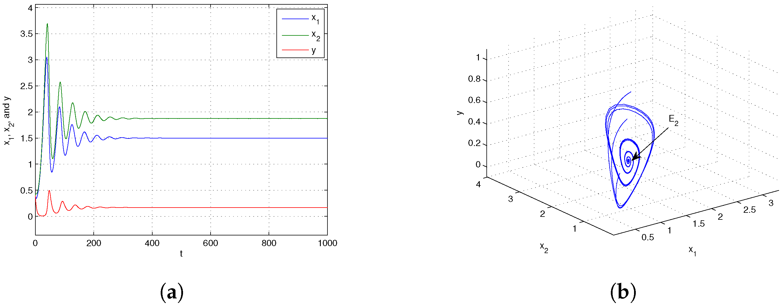
• Case I. Global stability of the equilibria

We first take the parameters of the system (6) as follows:

$$\alpha =0.4,s=0.5,d_1=0.5,d_2=0.3,\eta =0.2,k=0.15,r_1=1,r_2=0.3.$$

(21)

If we choose $\gamma =1,D_1=1.5,D_2=0.1,$ at this juncture, it can be demonstrated that $D_1>{\overline{D}}_1.$ By the conclusion of Theorem 7, it is known that the trivial equilibrium point $E_0(0,0,0)$ is globally asymptotically stable, which is shown in Figure 1. Next, when we choose $D_1=0.1,D_2=0.1,$ and $\gamma =1,$ from Figure 2, we know that the boundary equilibrium point $E_1(0.425,0.10625,0)$ is globally asymptotically stable. Choosing $D_1=0.5,D_2=0.2,$ and $\gamma =0.02,$ from Figure 3, we can obtain that the positive equilibrium $E_2(2.5,3.125,0.1335088457)$ is globally asymptotically stable.

When the dispersal is at an intermediate level, i.e., $0<D_1<{\overline{D}}_1$, the predator becomes extinct while the prey persists in both patches. The biological reason is that individuals that are extinguished in the sink patch are compensated by those moving from the source patch, which leads to the consumer’s persistence in both patches. However, when the prey’s dispersal from the source to sink is large (i.e., $D_1>{\overline{D}}_1$), the prey in both patches will be extinct. The underlying reason is that too many individuals move from the source patch to the sink patch. Therefore, appropriate dispersal promotes the persistence of the prey population.

• Case II. Total population abundance

When there is no dispersal (i.e., $D_1=D_2=0$), then $\underset{t\to +\infty }{lim}{x}_2\left(t\right)=0$. And system (6) becomes

$$\left\{\begin{array}{c}{\displaystyle \frac{d{x}_1}{dt}}={\displaystyle \frac{r_1{x}_1}{1+ky}}-d_1\left[1+\eta \left(1-{\displaystyle \frac{1}{1+ky}}\right)\right]x_1-\gamma x_1^2-\alpha x_{1}y,\hfill \\ {\displaystyle \frac{dy}{dt}}=sa{x}_{1}y-d_{2}y.\hfill \end{array}\right.$$

(22)

The system (22) has a globally asymptotically stable boundary equilibrium point $P_2\left({\displaystyle \frac{r_1-d_1}{\gamma }},0\right)$ if $f\left({\displaystyle \frac{r_1-d_1}{\gamma }}\right)<0$; in other words, $\underset{t\to +\infty }{lim}{x}_1\left(t\right)={\displaystyle \frac{r_1-d_1}{\gamma }}.$ We can denote the prey’s density as $T_0={\displaystyle \frac{r_1-d_1}{\gamma }}$.

Comparing the system (6) (with dispersal) to the system (22) (no dispersal), we see that all the solutions of system (6) converge to $E_1({\overline{x}}_1.{\overline{x}}_2,0)$ when $0<D_1<{\overline{D}}_1,f\left({\overline{x}}_1\right)<0$, which means that population densities of the prey are $T\left(D_1\right)=\left(1+{\displaystyle \frac{D_1}{r_2+D_2}}\right)\left({\displaystyle \frac{r_1-d_1-\frac{r_2{D}_1}{r_2+D_2}}{\gamma }}\right).$ We can draw the two curves of $T_0$ and T about $D_1$ in Figure 4. And we can obtain that $D_1^{\ast }={\displaystyle \frac{(r_2+D_2)(r_1-d_1-r_2)}{2r_2}},D_1^0=2D_1^{\ast }$ and $T_{max}=T\left(D_1^{\ast }\right).$ When $0<D_1<D_1^0=2D_1^{\ast },$ the density of the prey is larger than that without dispersal. Specifically, there exists an optimal dispersal coefficient (i.e., $D_1=D_1^{\ast }$) for maximizing the density of the prey (i.e., $T=T_{max}$). However, excessive dispersal (i.e., $D_1>D_1^0$) causes the density of the prey to be lower than that without dispersal. In particular, when the dispersal efficiency is large enough (i.e., $D_1\ge {\overline{D}}_1$), the prey goes extinct.

• Case III. Impact of fear effect on the system (6)

In order to understand the sensitivity of fear effect, we choose the same parameter set given in

$$\begin{array}{cc}\hfill \alpha & =0.4,s=0.5,d_1=0.5,d_2=0.3,\eta =0.2,k=0.15,r_1=1,r_2=0.3,\hfill \\ \hfill \gamma & =0.02,D_1=0.5,D_2=0.1.\hfill \end{array}$$

(23)

In Figure 5, we give the dynamical behavior of $x_1,x_2$ and y concerning time t for different levels of fear effect k, respectively. It can be observed that as the value of k increases, the stable levels of $x_1$ and $x_2$ in the system remain relatively unchanged. However, the amplitude of oscillations before reaching stability increases with the increase in k. Concurrently, the steady-state level of y significantly decreases. Figure 6 depicts the dynamics of $x_1,x_2$ and y with respect to time t for various values of $\eta$ which represents the maximum cost of fear. It is observed that as time progresses, for different $\eta$ values, $x_1,x_2$ and y all exhibit an initial decrease followed by an increase, ultimately oscillating towards the equilibrium state level. With an increase in $\eta$, the steady-state level of y decreases while the steady-state levels of $x_1$ and $x_2$ show no significant change. This indicates that a higher cost of prey fear towards predator results in a more pronounced impact on the predator population. Upon examining Figure 5 and Figure 6, we perceive that the fear effect exerts a negative impact on the population size of the predator y. Specifically, with an increase in the fear effect of the prey, the population of the predator y decreases, potentially leading to the ultimate extinction of the predator population.

8. Conclusions

In this paper, we analyze a predator-prey system with asymmetric dispersal and fear effect that affect the birth and death rates of prey species. We have the conclusions as follows.

• We first investigated the non-negativity and boundedness of system (6), and proved that system (6) is persistent if $0<k<k^{\ast }$. Furthermore, our research indicated that system (6) always has a trivial equilibrium point $E_0$, and in the case of $0<D_1<{\overline{D}}_1$, there exists a boundary equilibrium point $E_1$. Additionally, if condition $\left(H_1\right)$ holds, the system also possesses a unique positive equilibrium point $E_2$.
• When the parameter $D_1$ reaches or exceeds the critical value ${\overline{D}}_1$, the equilibrium $E_0(0,0,0)$ becomes globally asymptotically stable. Conversely, when $0<D_1<{\overline{D}}_1$ and $f\left({\overline{x}}_1\right)<0$, the boundary equilibrium point $E_1({\overline{x}}_1,{\overline{x}}_2,0)$ is globally asymptotically stable. By applying geometric methods, we further investigated the global asymptotic stability of the system around the equilibrium point $E_2$.
• When the parameter $D_1$ reaches the critical value ${\overline{D}}_1$, the boundary equilibrium point $E_1$ coincides with the trivial equilibrium point $E_0$, and a transcritical bifurcation occurs near $E_1$ with a switch in stability. As the dispersal rate $D_1$ approaches or exceeds the critical value ${\overline{D}}_1$, the migration of prey between habitat patches becomes extremely sensitive, potentially leading to species collapse. This finding provides crucial guidance for species conservation and habitat connectivity management. In the construction of ecological corridors, it is essential to ensure their effectiveness and prevent excessive dispersal of prey from source patches to sink patches, which is vital for preventing species extinction.
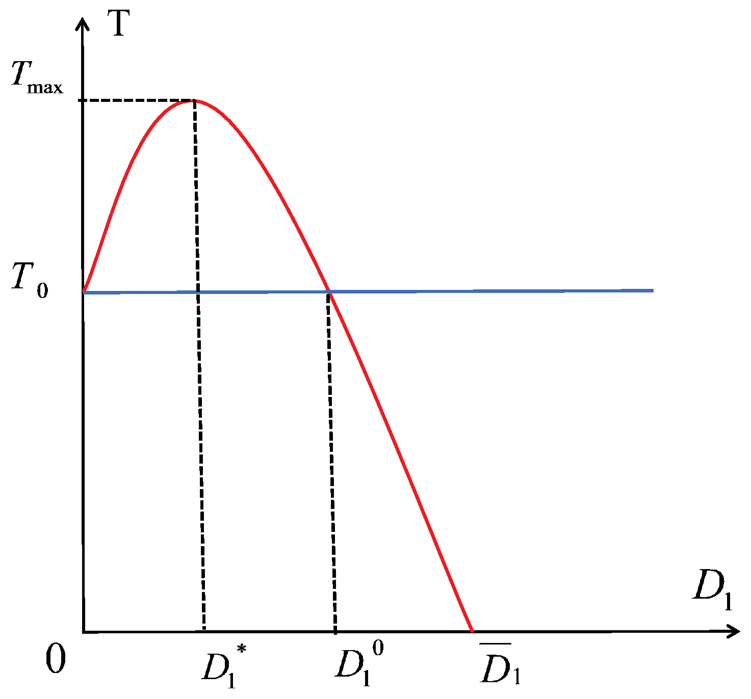
• Compared to the no-dispersal scenario, there is an optimal dispersal coefficient $D_1^{\ast }$ at which the prey population reaches its maximum. However, when $D_1$ exceeds $D_1^{\ast }$, the prey population begins to decline gradually. Upon reaching $D_1=D_1^0$, the prey population returns to the no-dispersal level, but as $D_1$ continues to increase, the prey population begins to fall below that of the no-dispersal case, eventually leading to extinction (see Figure 4).
• Next, we specifically investigated the impact of the fear effect parameter k and the maximum fear cost $\eta$ on the dynamics of system (6). Next, we specifically examined the effects of the fear effect parameter k and the maximum fear cost $\eta$ on the dynamics of system (6). Consistent with [42], our findings indicate that the fear effect reduces predator population density but does not alter the existence or stability of equilibrium points. However, with the introduction of maximum fear effects in our model, we further observed that higher maximum fear levels not only suppress predator density more significantly but may also accelerate population decline, potentially impacting the long-term stability of the ecosystem. From Figure 5 and Figure 6, it is evident that k and $\eta$ do not significantly affect the density of the prey but they lead to a continuous decrease in the final stable state of the predator.

In general, in our study, we are the first to introduce the maximum fear effect function into the source–sink predator-prey model, and we find that the dispersal of prey between source–sink patches is crucial for the total population size of prey. Additionally, both the fear effect parameter k and maximum fear cost $\eta$ have a negative impact on the population size of predators. In future research, we plan to explore other types of functional response functions and take into account the maximum fear effect for the prey’s birth rate. This study holds significant implications for the conservation of endangered species, as the establishment of ecological corridors has the potential to ultimately increase the population size of endangered species.

References

1. Chen, F.; Li, Z.; Pan, Q.; Zhu, Q. Bifurcations in a Leslie–Gower predator-prey model with strong Allee effects and constant prey refuges. Chaos Solitons Fractals 2025, 192, 115994. [Google Scholar] [CrossRef]
2. Ramasamy, S.; Banjerdpongchai, D.; Park, P. Stability and Hopf-bifurcation analysis of diffusive Leslie–Gower prey–predator model with the Allee effect and carry-over effects. Math. Comput. Simul. 2025, 227, 19–40. [Google Scholar] [CrossRef]
3. Zhong, J.; Chen, L.; Chen, F. Stability and bifurcation in a two-patch commensal symbiosis model with nonlinear dispersal and additive Allee effect. Int. J. Biomath. 2024, 2450099. [Google Scholar] [CrossRef]
4. Tang, D.; Ren, J. Bautin bifurcation with additive noise. Adv. Nonlinear Anal. 2022, 12, 20220277. [Google Scholar] [CrossRef]
5. Winkler, M. Application of the Moser–Trudinger inequality in the construction of global solutions to a strongly degenerate migration model. Bull. Math. Sci. World Sci. 2023, 13, 1. [Google Scholar] [CrossRef]
6. Alshehri, A.; Aljaber, N.; Altamimi, H.; Alessa, R.; Majdoub, M. Nonexistence of global solutions for a nonlinear parabolic equation with a forcing term. Opusc. Math. 2023, 43, 741–758. [Google Scholar] [CrossRef]
7. Wang, S.; Nie, L. Global stability and asymptotic profiles of a partially degenerate reaction diffusion Cholera model with asymptomatic individuals. Adv. Nonlinear Anal. 2024, 13, 20240059. [Google Scholar] [CrossRef]
8. Partohaghighi, M.; Akgül, A. New fractional modelling and simulations of prey–predator system with Mittag–Leffler kernel. Int. J. Appl. Comput. Math. 2023, 9, 43. [Google Scholar] [CrossRef]
9. Ahmad, Z.; Bonanomi, G.; Cardone, A.; Iuorio, A.; Toraldo, G.; Giannino, F. Fractal-fractional Sirs model for The disease dynamics in both prey and predator with singular and nonsingular kernels. J. Biol. Syst. 2024, 1–34. [Google Scholar] [CrossRef]
10. Kuipers, K.J.; Hilbers, J.P.; Garcia-Ulloa, J.; Graae, B.J.; May, R.; Verones, F.; Huijbregts, M.A.; Schipper, A.M. Habitat fragmentation amplifies threats from habitat loss to mammal diversity across the world’s terrestrial ecoregions. ONE Earth 2021, 4, 1505–1513. [Google Scholar] [CrossRef]
11. Tan, W.; Herrel, A.; Rödder, D. A global analysis of habitat fragmentation research in reptiles and amphibians: What have we done so far? Biodivers. Conserv. 2023, 32, 439–468. [Google Scholar] [CrossRef]
12. Tewksbury, J.J.; Levey, D.J.; Haddad, N.M.; Sargent, S.; Orrock, J.L.; Weldon, A.; Danielson, B.J.; Brinkerhoff, J.; Damschen, E.I.; Townsend, P. Corridors affect plants, animals, and their interactions in fragmented landscapes. Proc. Natl. Acad. Sci. USA 2002, 99, 12923–12926. [Google Scholar] [CrossRef]
13. Franco, D.; Ruiz-Herrera, A. To connect or not to connect isolated patches. J. Theor. Biol. 2015, 370, 72–80. [Google Scholar] [CrossRef]
14. Travers, E.; Härdtle, W.; Matthies, D. Corridors as a tool for linking habitats-Shortcomings and perspectives for plant conservation. J. Nat. Conserv. 2021, 60, 125974. [Google Scholar] [CrossRef]
15. Sun, X.; Shen, J.; Xiao, Y.; Li, S.; Cao, M. Habitat suitability and potential biological corridors for waterbirds in Yancheng coastal wetland of China. Ecol. Indic. 2023, 148, 110090. [Google Scholar] [CrossRef]
16. Freedman, H.; Waltman, P. Mathematical models of population interactions with dispersal. I: Stability of two habitats with and without a predator. SIAM J. Appl. Math. 1977, 32, 631–648. [Google Scholar] [CrossRef]
17. Arditi, R.; Lobry, C.; Sari, T. Is dispersal always beneficial to carrying capacity? New insights from the multi-patch logistic equation. Theor. Popul. Biol. 2015, 106, 45–59. [Google Scholar] [CrossRef] [PubMed]
18. Zhang, B.; Kula, A.; Mack, K.M.; Zhai, L.; Ryce, A.L.; Ni, W.M.; DeAngelis, D.L.; Van Dyken, J.D. Carrying capacity in a heterogeneous environment with habitat connectivity. Ecol. Lett. 2017, 20, 1118–1128. [Google Scholar] [CrossRef] [PubMed]
19. Holt, R.D. Population dynamics in two-patch environments: Some anomalous consequences of an optimal habitat distribution. Theor. Popul. Biol. 1985, 28, 181–208. [Google Scholar] [CrossRef]
20. Ruiz-Herrera, A.; Torres, P.J. Effects of diffusion on total biomass in simple metacommunities. J. Theor. Biol. 2018, 447, 12–24. [Google Scholar] [CrossRef] [PubMed]
21. Arditi, R.; Lobry, C.; Sari, T. Asymmetric dispersal in the multi-patch logistic equation. Theor. Popul. Biol. 2018, 120, 11–15. [Google Scholar] [CrossRef] [PubMed]
22. Wu, H.; Wang, Y.; Li, Y.; DeAngelis, D.L. Dispersal asymmetry in a two-patch system with source-sink populations. Theor. Popul. Biol. 2020, 131, 54–65. [Google Scholar] [CrossRef] [PubMed]
23. Ban, J.; Wang, Y.; Wu, H. Dynamics of predator-prey systems with prey’s dispersal between patches. Indian J. Pure Appl. Math. 2022, 53, 550–569. [Google Scholar] [CrossRef]
24. Preisser, E.L.; Bolnick, D.I.; Benard, M.F. Scared to death? The effects of intimidation and consumption in predator-prey interactions. Ecology 2005, 86, 501–509. [Google Scholar] [CrossRef]
25. Cresswell, W. Predation in bird populations. J. Ornithol. 2011, 152, 251–263. [Google Scholar] [CrossRef]
26. Suraci, J.P.; Clinchy, M.; Dill, L.M.; Roberts, D.; Zanette, L.Y. Fear of large carnivores causes a trophic cascade. Nat. Commun. 2016, 7, 10698. [Google Scholar] [CrossRef] [PubMed]
27. Zanette, L.Y.; White, A.F.; Allen, M.C.; Clinchy, M. Perceived predation risk reduces the number of offspring songbirds produce per year. Science 2011, 334, 1398–1401. [Google Scholar] [CrossRef] [PubMed]
28. Wang, X.; Zanette, L.; Zou, X. Modelling the fear effect in predator-prey interactions. J. Math. Biol. 2016, 73, 1179–1204. [Google Scholar] [CrossRef]
29. Sarkar, K.; Khajanchi, S. Impact of fear effect on the growth of prey in a predator-prey interaction model. Ecol. Complex. 2020, 42, 100826. [Google Scholar] [CrossRef]
30. Liu, T.; Chen, L.; Chen, F.; Li, Z. Dynamics of a Leslie-Gower model with weak Allee effect on prey and fear effect on predator. Int. J. Bifurc. Chaos 2023, 33, 2350008. [Google Scholar] [CrossRef]
31. Benamara, I.; El Abdllaoui, A. Bifurcation in a delayed predator-prey model with Holling type IV functional response incorporating hunting cooperation and fear effect. Int. J. Dyn. Control 2023, 11, 2733–2750. [Google Scholar] [CrossRef]
32. Sahoo, D.; Samanta, G. Impact of fear effect in a two prey-one predator system with switching behaviour in predation. Differ. Equ. Dyn. Syst. 2024, 32, 377–399. [Google Scholar] [CrossRef]
33. Li, Q.; Chen, F.; Chen, L.; Li, Z. Dynamical analysis of a discrete amensalism system with Michaelis–Menten type harvesting for the Second Species. Qual. Theory Dyn. Syst. 2024, 23, 1–43. [Google Scholar] [CrossRef]
34. Cai, Y.; Chen, Q.; Teng, Z.; Zhang, G.; Rifhat, R. Bifurcations in a discrete-time Beddington-DeAngelis prey-predator model with fear effect, prey refuge and harvesting. Nonlinear Dyn. 2025, 113, 931–969. [Google Scholar] [CrossRef]
35. Creel, S.; Christianson, D.; Liley, S.; Winnie, J.A., Jr. Predation risk affects reproductive physiology and demography of elk. Science 2007, 315, 960. [Google Scholar] [CrossRef]
36. Clinchy, M.; Sheriff, M.J.; Zanette, L.Y. Predator-induced stress and the ecology of fear. Funct. Ecol. 2013, 27, 56–65. [Google Scholar] [CrossRef]
37. Zanette, L.Y.; Clinchy, M. Ecology of fear. Curr. Biol. 2019, 29, R309–R313. [Google Scholar] [CrossRef] [PubMed]
38. Mukherjee, D. Role of fear in predator-prey system with intraspecific competition. Math. Comput. Simul. 2020, 177, 263–275. [Google Scholar] [CrossRef]
39. Das, B.K.; Sahoo, D.; Samanta, G. Impact of fear in a delay-induced predator-prey system with intraspecific competition within predator species. Math. Comput. Simul. 2022, 191, 134–156. [Google Scholar] [CrossRef]
40. Xue, Y.; Chen, F.; Xie, X.; Chen, S. An analysis of a predator-prey model in which fear reduces prey birth and death rates. AIMS Math. 2024, 9, 12906–12927. [Google Scholar] [CrossRef]
41. Das, B.K.; Sahoo, D.; Santra, N.; Samanta, G. Modeling predator-prey interaction: Effects of perceived fear and toxicity on ecological communities. Int. J. Dyn. Control 2024, 12, 2203–2235. [Google Scholar] [CrossRef]
42. Xia, Y.; Huang, X.; Chen, F.; Chen, L. Stability and bifurcation of a predator-prey system with multiple anti-predator behaviors. J. Biol. Syst. 2024, 32, 889–919. [Google Scholar] [CrossRef]
43. Perko, L. Differential Equations and Dynamical Systems; Springer: Berlin/Heidelberg, Germany, 2013; Volume 7. [Google Scholar]
44. Miller, R.K.; Michel, A.N. Ordinary Differential Equations; Academic Press: Cambridge, MA, USA, 2014. [Google Scholar]
45. Li, M.Y.; Muldowney, J.S. Global stability for the SEIR model in epidemiology. Math. Biosci. 1995, 125, 155–164. [Google Scholar] [CrossRef]
46. Li, M.Y.; Muldowney, J.S. A geometric approach to global-stability problems. SIAM J. Math. Anal. 1996, 27, 1070–1083. [Google Scholar] [CrossRef]
47. Lidicker, W. The role of dispersal in the demography of small mammals. In Small Mammals: Productivity and Dynamics of Populations; Cambridge University Press: Cambridge, UK, 1975; pp. 103–128. [Google Scholar]
48. Baxter, C.V.; Fausch, K.D.; Carl Saunders, W. Tangled webs: Reciprocal flows of invertebrate prey link streams and riparian zones. Freshw. Biol. 2005, 50, 201–220. [Google Scholar] [CrossRef]
49. Birkhoff, G.; Rota, G. Ordinary Differential Equation; Ginn and Co.: Boston, MA, USA, 1982. [Google Scholar]
50. Wang, Z.; Wang, Y. Bifurcations in diffusive predator-prey systems with Beddington-DeAngelis functional response. Nonlinear Dyn. 2021, 105, 1045–1061. [Google Scholar] [CrossRef]
51. Senan, N.A.F. A Brief Introduction to Using ode45 in MATLAB; University of California: Berkeley, MA, USA, 2007. [Google Scholar]
Figure 1. (a) Time phase of model (6) around E 0 , where γ = 1 , D 1 = 1.5 , D 2 = 0.1 . (b) Phase portrait of E 0 . The relevant parameter values are given in (21).
Symmetry 17 00329 g001
Figure 2. (a) Time phase of model (6) around E 1 , where γ = 1 , D 1 = 0.1 , D 2 = 0.1 . (b) Phase portrait of E 1 . The relevant parameter values are given in (21).
Symmetry 17 00329 g002
Figure 3. (a) Time phase of model (6) around E 2 , where γ = 0.02 , D 1 = 0.5 , D 2 = 0.1 . (b) Phase portrait of E 2 . The relevant parameter values are given in (21).
Symmetry 17 00329 g003
Figure 4. Curves of prey population density about D 1 . The blue straight line represents the population density of prey without dispersal, whereas the red curve represents prey population density with dispersal.
Symmetry 17 00329 g004
Figure 5. (a) Trajectory of x 1 . (b) Trajectory of x 2 . (c) Trajectory of y. Trajectories of x 1 , x 2 and y with respect to time t for different values of k and others parameters chosen in (23).
Symmetry 17 00329 g005
Figure 6. (a) Trajectory of x 1 . (b) Trajectory of x 2 . (c) Trajectory of y. Trajectories of x 1 , x 2 and y with respect to time t for different values of η and others parameters chosen in (23).
Symmetry 17 00329 g006