Robust Discriminative Non-Negative and Symmetric Low-Rank Projection Learning for Feature Extraction

Abstract

Feature extraction plays a vital role in pattern recognition and computer vision. In recent years, low-rank representation (LRR) has been widely used in feature extraction, due to its robustness against noise. However, existing methods often overlook the impact of a well-constructed low-rank coefficient matrix on projection learning. This paper introduces a novel feature extraction method, i.e., robust discriminative non-negative and symmetric low-rank projection learning (RDNSLRP), where a coefficient matrix with better properties, such as low-rank, non-negativity, symmetry and block-diagonal structure, is utilized as a graph matrix for learning the projection matrix. Additionally, a discriminant term is introduced to increase inter-class divergence while decreasing intra-class divergence, thereby extracting more discriminative features. An iterative algorithm for solving the proposed model was designed by using the augmented Lagrange multiplier method, and its convergence and computational complexity were analyzed. Our experimental results on multiple data sets demonstrate the effectiveness and superior image-recognition performance of the proposed method, particularly on data sets with complex intrinsic structures. Furthermore, by investigating the effects of noise corruption and feature dimension, the robustness against noise and the discrimination of the proposed model were further verified.

1. Introduction

Massive amounts of high-dimensional data, such as text, image, video frame and biological information, are broadly used in our daily lives and in scientific research. However, direct processing of such extensive high-dimensional data can lead to a severe problem, known as the “curse of dimensionality”. Therefore, feature extraction from high-dimensional data has become a prominent research topic in recent years. Over the past few decades, a number of feature extraction methods have been proposed, among which principle component analysis (PCA) [1] is particularly noteworthy. As an unsupervised feature extraction method, PCA seeks a low-dimensional orthogonal projection matrix via minimizing reconstruction errors. However, PCA can barely process data that are heavily corrupted by complex noise [2]. The proposal of low-rank representation (LRR) [3,4] effectively solved this problem by better-capturing the global structure within the original data while removing noise and outliers. Recently, LRR has received much attention in machine learning and computer vision, and its variants have been successfully applied to different scenarios, including feature selection [5,6,7] and subspace clustering [8,9]. However, the absence of a projection matrix limits LRR’s ability to effectively deal with feature extraction tasks, and recent research has focused mainly on three strategies to address this limitation:

(1) The first strategy extracts intrinsic features by employing a low-rank projection matrix, with latent low-rank representation (LatLRR) [10] and double low-rank representation (DLRR) [11] being representative examples. However, the feature dimensions of the projection matrices obtained through LatLRR, DLRR and their variants [12,13,14] remain identical to the original data, and their efficiency in handling high-dimensional data is thereby severely limited. Approximate low-rank projection learning (ALPL) [15] and its variants [16,17] have effectively solved this problem by decomposing the low-rank projection matrix into an orthogonal transformation matrix and a low-dimensional projection matrix, thus realizing the projection of high-dimensional features into lower-dimensional subspaces. Nonetheless, these methods tend to overlook the manifold structure of the original data, which is essential to preserving the distribution of data that belong to the same class in the low-dimensional subspaces. In addition, the norm type used to constrain the projection matrix (such as Frobenius norm and $l_{2,1}$ norm) has a significant impact on the feature extraction performance, requiring the assumption of coefficient distribution in the model’s construction process.

(2) The second strategy is to introduce sparse constraint into the low-rank representation model, extracting local features from the original data by the self-representation property of sparse matrices. Low-rank sparse representation (LRSR) [18] is a prominent method primarily utilized in subspace clustering and segmentation, which has been successfully extended to feature extraction [19,20]. However, sparse representation may result in feature loss, to some extent, and the feature extraction methods based on this strategy still cannot fully consider the manifold structure of the original data samples. Recently, a discriminative feature extraction method (DFE) [21] proposed by Liu et al. enhanced LRSR by introducing a low-dimensional projection matrix to solve the out-of-sample problem and a discriminative term to minimize the reconstruction error of the original data. However, the learning of a projection matrix does not facilitate a mutual reinforcement of the learning of a sparse low-rank coefficient matrix.

(3) The third strategy focuses on non-linear and manifold structures, employing local preserving projection (LPP) [22] or graph learning to preserve the intrinsic structures of the original data. Low-rank preserving projection (LRPP) [23] and low-rank representation with adaptive graph regularization (LRR_AGR) [24] are representatives, which are capable of identifying the intrinsic manifold structure of the data and retaining local information. Low-rank preserving projection via graph regularized reconstruction (LRPP_GRR) [25] combines graph constraint on the reconstruction error of data with projection learning to further improve its classification accuracy and robustness against noise. However, most graph matrix-based learning methods typically preconstruct affinity or k-nearest neighbor graphs using original data samples, which often contain noise corruption and outliers in real-world applications. Furthermore, since Euclidean distances are sensitive to noise corruption, the preconstructed graph matrices often fail to accurately capture the correlation between two data samples.

Recently, a number of studies have integrated and improved upon these strategies, and more effective methods have been proposed to address the limitations and enhance the performance of feature extraction. For example, robust latent discriminative adaptive graph preserving learning (RLDAGP) [26] integrates adaptive graph learning with dimensionality reduction, meanwhile incorporating an adaptive regularizer to better-accommodate data sets with diverse characteristics. Moreover, adaptive graph embedding preserving projection learning (AGE_PPL) [27] combines adaptive sparse graph learning, global structure preservation and projection learning, thereby preserving both the global and local structures of data, which significantly improves the effectiveness of feature extraction. However, several drawbacks remain despite the success of the existing methods for feature extraction tasks. Firstly, most feature extraction methods ignore the significant role that a low-rank coefficient matrix with favorable properties can play in learning projection matrices. Theoretically, a well-structured graph matrix $\mathbf{Z}$ should facilitate projection matrix learning. Secondly, many adaptive graph learning-based methods still rely on the preconstruction of graph matrices, and the accuracy of the graph depends on the size of the predetermined neighborhood k, which cannot adequately meet the diverse requirements of different image data sets. Last but not least, the objective functions of these models are specially designed and tend to be more complex, making it difficult for these models to scale among different learning scenarios. For example, in practical applications, there are several internal parameters that require additional adjustment (such as $\alpha$ in [26]) in addition to the regularization parameters, greatly increasing the effort required to find an optimal parameter combination.

In order to address these drawbacks, a novel method, i.e., the robust discriminative non-negative and symmetric low-rank projection learning method (RDNSLRP), is proposed. RDNSLRP optimizes low-rank representation to non-negative symmetric low-rank representation, and it applies block-diagonal properties to construct a low-rank coefficient matrix with better properties to improve the interpretability of the model. By integrating non-negative symmetric low-rank representation and adaptive graph learning into a unified framework, RDNSLRP can extract more geometric intrinsic features from the original data. Meanwhile, the projection matrix learned from a low-rank coefficient matrix with better properties (such as non-negative, symmetric and block diagonal) is expected to be more discriminative than that from the unconstrained matrix. In addition, a discriminant term based on the projection error of each class is also introduced to increase intra-class divergence while decreasing inter-class divergence, thereby learning a more discriminative projection matrix. The main contributions of this paper are summarized as follows:

• RDNSLRP introduces a low-dimensional projection matrix and adaptive graph learning to low-rank representation, enabling the local geometric structures of the original data to be projected to lower-dimensional subspaces while extracting both the global and intrinsic features.
• A low-rank coefficient matrix with better properties, such as non-negative, symmetric and block-diagonal, is introduced as a graph matrix for adaptive graph learning to enhance interpretability and achieve mutual promotion during the learning process between the graph matrix and the projection matrix.
• A discriminant term based on the projection error of each sample class is designed and utilized to further enhance the discriminability of feature extraction.
• To resolve the RDNSLRP model, an alternating iteration algorithm based on the augmented Lagrange multiplier method with alternating direction strategy is designed, and a restrictive method is used to ensure the block-diagonal property of the graph matrix.
• Comprehensive experiments conducted on benchmark data sets have proved the effectiveness and practicality of the RDNSLRP model.

The remainder of this paper consists of the following sections. In Section 2 , the notations are introduced and related methods are briefly discussed. Section 3 introduces the formulation of the RDNSLRP model, and its optimization procedure and application of feature extraction are given. Section 4 proves the convergence and discusses the complexities of the proposed model. Our experimental results and correlation analyses are presented in Section 5. Section 6 lists some limitations of the proposed method and looks forward to possible future work. Section 7 summarizes the contents of the paper.

2. Notations and Fundamental Models

This section first introduces some notations and then reviews some fundamental models related to this work, including graph regularization-based manifold learning, low-rank representation and its variants.

2.1. Notations

In this paper, matrices are represented by bold uppercase letters, vectors are represented by bold lowercase letters and numeric variables are represented by normal lowercase letters. For a vector s = $[s_1,s_2,\dots ,s_n]$, the $l_2$ norm is defined as ${\parallel \mathbf{s}\parallel }_2=\sqrt{{\sum }_{i=1}^n{s}_i^2}$. For the matrix $\mathbf{A}\in {\mathbb{R}}^{p\times q}$, ${\mathbf{A}}^T$ represents the transposed matrix of matrix $\mathbf{A}$, $rank\left(\mathbf{A}\right)$ represents the rank function of matrix $\mathbf{A}$ and $tr\left(\mathbf{A}\right)$ represents the trace function only when $p=q$. Let $a_{ij}$ be the element at the i-th row and j-th column of matrix $\mathbf{A}$; the norms of $\mathbf{A}$ are defined as follows:

• The $l_1$ norm of matrix $\mathbf{A}$ is defined as ${\parallel \mathbf{A}\parallel }_1={\sum }_{i=1}^p{\sum }_{j=1}^q\left|a_{ij}\right|$.
• The $l_{2,1}$ norm of matrix $\mathbf{A}$ is defined as ${\parallel \mathbf{A}\parallel }_{2,1}={\sum }_{j=1}^q\sqrt{{\sum }_{i=1}^p{a}_{ij}^2}$.
• The Frobenius norm of matrix $\mathbf{A}$ is defined as ${\parallel \mathbf{A}\parallel }_F=\sqrt{{\sum }_{i=1}^p{\sum }_{j=1}^q{a}_{ij}^2}$.
• The nuclear norm of matrix $\mathbf{A}$ is defined as ${\parallel \mathbf{A}\parallel }_{\ast }={\sum }_{i=1}^{rank\left(\mathbf{A}\right)}{\sigma }_i$, where ${\sigma }_i$ denotes the i-th non-zero singular value of matrix $\mathbf{A}$, $i=1,2,\dots ,rank\left(\mathbf{A}\right)$.

2.2. Graph Regularization-Based Manifold Learning

The neighbor graph is widely used to reveal the geometric structure among samples, and it has extensive applications in feature extraction and selection tasks [22,28]. For the given data matrix $\mathbf{X}=[{\mathbf{x}}_1,{\mathbf{x}}_2,\dots ,{\mathbf{x}}_n]\in {\mathbb{R}}^{m\times n}$, the graph regularization-based manifold learning method initially constructs a nearest neighbor graph $\mathbf{W}\in {\mathbb{R}}^{n\times n}$ to capture the local relationship among samples, and it then conducts projection learning by solving the subsequent optimization problem,

$$\underset{{\mathbf{P}}^T{\mathbf{XX}}^T\mathbf{P}={\mathbf{I}}_d}{min}\sum _{i,j}{\parallel {\mathbf{P}}^T{\mathbf{x}}_i-{\mathbf{P}}^T{\mathbf{x}}_j\parallel }_2^2{w}_{ij},$$

(1)

where $\mathbf{P}\in {\mathbb{R}}^{m\times d}$ denotes the projection matrix. In recent years, numerous construction methods for the nearest neighbor graph matrix $\mathbf{W}$ have been proposed by researchers. Among them, a rather straightforward approach called Heatkernel is to define each element $w_{ij}$ of the graph matrix $\mathbf{W}$ as follows:

$$w_{ij}=\left\{\begin{array}{ll}\exp \left(-{\displaystyle \frac{\parallel {\mathbf{x}}_i-{\mathbf{x}}_j{\parallel }^2}{2{\sigma }^2}}\right),& \mathrm{if}{\mathbf{x}}_i\in N_k\left({\mathbf{x}}_j\right)\mathrm{or}{\mathbf{x}}_j\in N_k\left({\mathbf{x}}_i\right)\hfill \\ 0,\hfill & \mathrm{otherwise},\hfill \end{array}\right.$$

(2)

where $N_k\left({\mathbf{x}}_j\right)$ denotes the set of k-nearest neighbor samples of ${\mathbf{x}}_j$, and where $\sigma$ is a bandwidth parameter that affects the rate at which the weights decay. The value of $w_{ij}$, as determined by the above construction function, is related to the Euclidean distance between ${\mathbf{x}}_i$ and ${\mathbf{x}}_j$, which means their similarity. Specifically, higher similarity between ${\mathbf{x}}_i$ and ${\mathbf{x}}_j$ will lead to a smaller Euclidean distance, thereby resulting in a larger weight of corresponding $w_{ij}$, and vice versa. Conversely, a relatively high weight of $w_{ij}$ also implies that the two samples ${\mathbf{x}}_i$ and ${\mathbf{x}}_j$ are similar and have a higher probability of belonging to the same class. Through this construction, the graph matrix $\mathbf{W}$ is able to express the intrinsic structural information of the original data, to some extent, and to further capture the essential local information of the original data during the LPP learning [22].

2.3. Low-Rank Representation Learning

The rank of a matrix represents the maximum number of uncorrelated vectors, and it is generally used to measure the correlation between the rows and columns of a matrix. When the rows or columns of the data samples exhibit strong correlations, it can be effectively represented by a lower-rank matrix and projected into a lower-dimensional linear subspace. We assume that the original data samples $\mathbf{X}=[{\mathbf{x}}_1,{\mathbf{x}}_2,\dots ,{\mathbf{x}}_n]\in {\mathbb{R}}^{m\times n}$ are approximately drawn from a mixture of multiple low-rank subspaces; the core concept of low-rank representation (LRR) [3,4] is to reveal the inherent low-dimensional structure within the data by constructing a low-rank coefficient matrix $\mathbf{Z}$, so that the linear relationships among the data points in the original data (namely, the global structure) can be precisely captured. LRR aims to solve the following problem:

$$\underset{\mathbf{Z}}{min}rank\left(\mathbf{Z}\right)s.t.\mathbf{X}=\mathbf{XZ}.$$

(3)

However, due to the discrete nature of rank constraint, problem (3) is essentially an NP-hard problem. A common agent in rank minimization problems is to replace the rank function with the nuclear norm function [29], which transforms problem (3) into the following convex optimization problem:

$$\underset{\mathbf{Z}}{min}{\parallel \mathbf{Z}\parallel }_{\ast }s.t.\mathbf{X}=\mathbf{XZ}.$$

(4)

In practical applications, the influence of errors and outliers is inevitable and must be taken into account. We denote $\mathbf{E}\in {\mathbb{R}}^{m\times n}$ as the sparse noise matrix of the original data matrix and $\lambda >0$ as the regularization parameter; LRR evolves into the following form for effectively separating noise and outliers:

$$\underset{\mathbf{Z},\mathbf{E}}{min}{\parallel \mathbf{Z}\parallel }_{\ast }+\lambda {\parallel \mathbf{E}\parallel }_{2,1}s.t.\mathbf{X}=\mathbf{XZ}+\mathbf{E}.$$

(5)

The low-rank constraint on the coefficient matrix $\mathbf{Z}$ ensures that the coefficients of samples coming from the same subspace exhibit high correlation, with each element $z_{ij}$ denoting the interaction between data points ${\mathbf{x}}_i$ and ${\mathbf{x}}_j$. However, the values of $z_{ij}$ and $z_{ji}$ are not necessarily equivalent in actual applications, which may undermine the interpretability of the model. To maintain weight consistency for each pair of data points, Chen et al. proposed a low-rank representation model with a symmetry constraint [30],

$$\underset{\mathbf{Z},\mathbf{E}}{min}{\parallel \mathbf{Z}\parallel }_{\ast }+\lambda {\parallel \mathbf{E}\parallel }_{2,1}s.t.\mathbf{X}=\mathbf{XZ}+\mathbf{E},\mathbf{Z}={\mathbf{Z}}^T,$$

(6)

which can effectively preserve the subspace structures of high-dimensional data, while ensuring that highly correlated data points within the subspaces are co-represented.

3. Proposed RDNSLRP Model

This section first describes the research motivation of this paper in detail, and then formulates the proposed RDNSLRP model. In addition, an algorithm is designed for optimization to solve the proposed model, and the method of feature extraction is given.

3.1. Motivation and Model Formulation

Most graph-based methods rely on k-nearest neighbor (KNN) or other techniques to preconstruct a neighbor graph or Laplacian graph. However, the accuracy of these graphs depends on a predefined neighborhood k, which cannot be adaptively learned from the original data. Consequently, pairwise data relationships may be inaccurate and inconsistent. Therefore, non-negative and symmetric constraints are applied to eliminate the influence of negative elements in $\mathbf{Z}$, thereby maintaining the weight consistency for each pair of data and increasing the interpretability of the model [31]. In addition, the main diagonal elements of $\mathbf{Z}$ are set to 0 to eliminate the self-representation effect, resulting in the following low-rank representation model with non-negative and symmetric constraints:

$$\begin{array}{c}\hfill \underset{\mathbf{Z},\mathbf{E}}{min}{\parallel \mathbf{Z}\parallel }_{\ast }+\lambda {\parallel \mathbf{E}\parallel }_{2,1}s.t.\mathbf{X}=\mathbf{XZ}+\mathbf{E},\mathbf{Z}={\mathbf{Z}}^T,\mathbf{Z}\ge \mathbf{0},z_{ii}=0.\end{array}$$

(7)

In addition, projection, which has been demonstrated to be an effective way to obtain better features, maps the data from the original space into a new lower-dimensional subspace, thereby reducing the effect of noise corruption while preserving the essential structural features. Manifold learning based on graph regularization has demonstrated efficiency in learning projections, so (1) can be introduced to model (7) for constructing the projection matrix. Moreover, as is mentioned in Section 2, each element $z_{ij}$ of the coefficient matrix $\mathbf{Z}$ represents the interaction between data ${\mathbf{x}}_i$ and ${\mathbf{x}}_j$; therefore, the coefficient matrix $\mathbf{Z}$ can be served as a graph matrix for adaptive learning. Through this construction, the learning of graph matrix $\mathbf{Z}$ and projection matrix $\mathbf{P}$ can be mutually promoted to each other and updated to the optimum. Meanwhile, a projection representation error term $\parallel {\mathbf{P}}^T\mathbf{X}-{\mathbf{P}}^T{\mathbf{XZ}\parallel }_F^2$ is introduced to (7) to reduce the interference of noise corruption [8], and the following model is constructed:

$$\begin{array}{cc}\hfill & \underset{\mathbf{Z},\mathbf{P}}{min}\sum _{i,j}\parallel {\mathbf{P}}^T{\mathbf{x}}_i-{\mathbf{P}}^T{\mathbf{x}}_j{\parallel }_2^2{z}_{ij}+{\alpha \parallel \mathbf{Z}\parallel }_{\ast }+{\displaystyle \frac{\beta }{2}}{\parallel {\mathbf{P}}^T\mathbf{X}-{\mathbf{P}}^T\mathbf{XZ}\parallel }_F^2\hfill \\ \hfill & s.t.\mathbf{Z}={\mathbf{Z}}^T,\mathbf{Z}\ge \mathbf{0},z_{ii}=0,{\mathbf{P}}^T\mathbf{P}={\mathbf{I}}_d,\hfill \end{array}$$

(8)

where $\mathbf{P}\in {\mathbb{R}}^{m\times d}$ is a projection matrix with an orthogonal constraint imposed to minimize data redundancy and avoid trivial solutions, and where $\alpha$, $\beta$ are non-negative regularized parameters. According to (8), $\parallel {\mathbf{P}}^T{\mathbf{x}}_i-{\mathbf{P}}^T{\mathbf{x}}_j{\parallel }_2^2$ denotes the distance between two distinct samples projected into the low-dimensional feature subspace, which serves to constrain the local neighborhood preservation, and $z_{ij}$ can be used to measure the similarity between samples ${\mathbf{x}}_i$ and ${\mathbf{x}}_j$, thereby preserving the local structure of the data. Specifically, higher similarity between ${\mathbf{x}}_i$ and ${\mathbf{x}}_j$ results in a larger value of $z_{ij}$, while higher dissimilarity leads to a smaller value of $z_{ij}$ (as well as $z_{ji}$). Combined with the introduction of the constraints, the adaptive-learned graph matrix $\mathbf{Z}$ is supposed to have better properties.

Furthermore, according to the principle of LRR, an ideal representation matrix should have a c-block-diagonal structure [3,4], where c represents the number of classes of training samples. However, in practical applications, maintaining the block-diagonal structure is challenging, especially when the original data set is contaminated by severe noise or outliers, which leads to the irrelevant components of the coefficient matrix participating in the reconstruction of a certain class of samples. To address this problem and further improve the model’s recognition performance, samples from training data ${\mathbf{X}}_s$ that belong to class s are constrained to be represented only by their corresponding submatrix ${\mathbf{Z}}_s$, rather than by the other parts of $\mathbf{Z}$. In addition, by introducing the projection matrix and fully utilizing its information, the discriminant term is formulated as follows:

$$\begin{array}{cc}\hfill & D(\mathbf{P},\mathbf{Z})=\sum _{s=1}^c\left(\parallel {\mathbf{P}}^T{\mathbf{X}}_s-{\mathbf{P}}^T{\mathbf{X}}_s{\mathbf{Z}}_s{\parallel }_F^2+\sum _{j=1,j\ne s}^c{\parallel {\mathbf{P}}^T{\mathbf{X}}_s{\mathbf{Z}}_j\parallel }_F^2\right)\hfill \\ \hfill & \mathbf{Z}=diag({\mathbf{Z}}_1,{\mathbf{Z}}_2,\dots ,{\mathbf{Z}}_c),{\mathbf{Z}}_s\in {\mathbb{R}}^{n_s\times n_s},\sum _{s=1}^c{n}_s=n.\hfill \end{array}$$

(9)

The discriminant term (9) only uses the submatrix ${\mathbf{Z}}_s$ to participate in the reconstruction process of ${\mathbf{X}}_s$, while minimizing the influence of other parts of $\mathbf{Z}$, ensuring that the information within the block-diagonal parts of $\mathbf{Z}$ is effectively utilized during the learning process. By introducing constraints on the block-diagonal structure of $\mathbf{Z}$, intra-class divergence is reduced while inter-class divergence is increased, so that the discrimination of feature subspaces is improved. It can be observed from Figure 1 that the discriminant term enables the model to possess a stronger discriminative ability. In addition, the first term of (9) can be regarded as the projection representation error of each class, so the projection representation term can be replaced by (9), obtaining the following robust discriminant non-negative and symmetric low-rank projection learning (RDNSLRP) model:

$$\begin{array}{cc}\hfill & \underset{\mathbf{Z},\mathbf{P}}{min}\sum _{i,j}\parallel {\mathbf{P}}^T{\mathbf{x}}_i-{\mathbf{P}}^T{\mathbf{x}}_j{\parallel }_2^2{z}_{ij}+\alpha {\parallel \mathbf{Z}\parallel }_{\ast }+{\displaystyle \frac{\beta }{2}}D(\mathbf{P},\mathbf{Z})\hfill \\ \hfill & s.t.\mathbf{Z}={\mathbf{Z}}^T,\mathbf{Z}\ge \mathbf{0},z_{ii}=0,{\mathbf{P}}^T\mathbf{P}={\mathbf{I}}_d.\hfill \end{array}$$

(10)

The RDNSLRP model integrates non-negative and symmetric low-rank representation, adaptive graph learning and discriminant projection learning into a unified framework, aiming to extract both global and local features of the data. By constructing a coefficient matrix $\mathbf{Z}$ with better properties to guide the learning of the projection matrix $\mathbf{P}$ and by weakening the influence of noise and outliers, the robustness and discrimination of the feature extraction is improved. Otherwise, the RDNSLRP model is capable of extending to supervised learning scenarios by incorporating label information through several methods, such as linear regression (LRC) [32] and discriminant least squares regression (DLSR) [33].

3.2. Model Optimization

According to the proposed model (10), there are two unknown block variables ($\mathbf{Z}$ and $\mathbf{P}$) that need to be optimized. By introducing two auxiliary variables, $\mathbf{S}$ and $\mathbf{J}$, (10) becomes separable and can be formulated as

$$\begin{array}{cc}\hfill & \underset{\mathbf{Z},\mathbf{P},\mathbf{S},\mathbf{J}}{min}\sum _{i,j}\parallel {\mathbf{P}}^T{\mathbf{x}}_i-{\mathbf{P}}^T{\mathbf{x}}_j{\parallel }_2^2{s}_{ij}+\alpha {\parallel \mathbf{Z}\parallel }_{\ast }+{\displaystyle \frac{\beta }{2}}D(\mathbf{P},\mathbf{J})\hfill \\ \hfill & s.t.\mathbf{Z}=\mathbf{S},\mathbf{Z}=\mathbf{J},\mathbf{S}={\mathbf{S}}^T,\mathbf{S}\ge \mathbf{0},s_{ii}=0,{\mathbf{P}}^T\mathbf{P}={\mathbf{I}}_d.\hfill \end{array}$$

(11)

Although the objective function of (11) is non-convex for all variables and is difficult to be solved directly, it is convex when one variable is unknown and other variables are known. Therefore, (11) can be solved by an augmented Lagrange multiplier (ALM) with an alternating direction minimizing (ADM) strategy [34]. Specifically, ALM-ADM strategy enables the model to be optimized in a way that iteratively updates each block variable one by one. Among them, variable $\mathbf{S}$ is introduced to ensure the overall properties of the graph matrix, such as non-negativity and symmetry, and, therefore, it is expected to be updated as a whole. Variable $\mathbf{J}$, on the other hand, is introduced for the reconstruction of each class of data samples, which requires it to be divided into several sub-matrices for separate updates. Moreover, by imposing equivalent constraints, it can be ensured that the updated graph $\mathbf{Z}$ simultaneously possesses the desirable properties of both auxiliary variables. To this end, the augmented Lagrange function of problem (11) can be defined as the following format:

$$\begin{array}{cc}\hfill & L(\mathbf{Z},\mathbf{P},\mathbf{S},\mathbf{J},{\mathbf{Y}}_1,{\mathbf{Y}}_2)=\sum _{i,j}\parallel {\mathbf{P}}^T{\mathbf{x}}_i-{\mathbf{P}}^T{\mathbf{x}}_j{\parallel }_2^2{s}_{ij}+\alpha {\parallel \mathbf{Z}\parallel }_{\ast }\hfill \\ \hfill & +{\displaystyle \frac{\beta }{2}}D(\mathbf{P},\mathbf{J})+{\displaystyle \frac{\mu }{2}}\left(\parallel \mathbf{Z}-\mathbf{S}+{\displaystyle \frac{{\mathbf{Y}}_1}{\mu }}{\parallel }_F^2+\parallel \mathbf{Z}-\mathbf{J}+{\displaystyle \frac{{\mathbf{Y}}_2}{\mu }}{\parallel }_F^2\right),\hfill \end{array}$$

(12)

where ${\mathbf{Y}}_1$ and ${\mathbf{Y}}_2$ are Lagrange multiplier matrices and $\mu >0$ is a penalty parameter. Then, (11) can be rewritten as the following constrained optimization problem:

$$\underset{\mathbf{Z},\mathbf{P},\mathbf{S},\mathbf{J}}{min}L(\mathbf{Z},\mathbf{P},\mathbf{S},\mathbf{J},{\mathbf{Y}}_1,{\mathbf{Y}}_2)s.t.\mathbf{S}={\mathbf{S}}^T,\mathbf{S}\ge \mathbf{0},s_{ii}=0,{\mathbf{P}}^T\mathbf{P}={\mathbf{I}}_d.$$

(13)

Therefore, the alternating iteration method for solving problem (13) is an iterative optimization process of alternately updating one of the block variables while fixing others. The updating rules of the block variables in each iteration are given below, in detail:

• Updating $\mathbf{P}$
  When $\mathbf{P}$ is unknown and other variables are fixed, the problem of minimizing (13) becomes the following optimization problem, after some irrelevant terms are removed:

  $$\underset{\mathbf{P}}{min}\sum _{i,j}{\parallel {\mathbf{P}}^T{\mathbf{x}}_i-{\mathbf{P}}^T{\mathbf{x}}_j\parallel }_2^2{s}_{ij}+{\displaystyle \frac{\beta }{2}}D(\mathbf{P},\mathbf{J})s.t.{\mathbf{P}}^T\mathbf{P}={\mathbf{I}}_d.$$

  (14)
  For the first term of (14), the following equivalence relationship can be obtained:

  $$\sum _{i,j}{\parallel {\mathbf{P}}^T{\mathbf{x}}_i-{\mathbf{P}}^T{\mathbf{x}}_j\parallel }_2^2{s}_{ij}=tr\left({\mathbf{P}}^T{\mathbf{XLX}}^T\mathbf{P}\right),$$

  (15)

  where the Laplacian matrix $\mathbf{L}=\mathbf{D}-\mathbf{S}$ and each element of the diagonal matrix $\mathbf{D}$ satisfies $d_{ii}={\sum }_{j=1}^n{s}_{ij}$ and $d_{ik}=0,i\ne k$. Denoting ${\mathbf{B}}_1={\sum }_{s=1}^c({\mathbf{X}}_s-{\mathbf{X}}_s{\mathbf{J}}_s)$, ${\mathbf{B}}_2={\sum }_{s=1}^c{\sum }_{j=1,j\ne s}^c{\mathbf{X}}_s{\mathbf{J}}_j$, the second term of (14) can be converted to the following format:

  $$D(\mathbf{P},\mathbf{J})=\parallel {\mathbf{P}}^T{\mathbf{B}}_1{\parallel }_F^2+{\parallel {\mathbf{P}}^T{\mathbf{B}}_2\parallel }_F^2=tr\left({\mathbf{P}}^T{\mathbf{B}}_1{\mathbf{B}}_1^T\mathbf{P}\right)+tr\left({\mathbf{P}}^T{\mathbf{B}}_2{\mathbf{B}}_2^T\mathbf{P}\right),$$

  (16)

  and (14) can thereby be rewritten as the following problem:

  $$\underset{\mathbf{P}}{min}tr\left({\mathbf{P}}^T{\mathbf{XLX}}^T\mathbf{P}\right)+{\displaystyle \frac{\beta }{2}}tr\left[{\mathbf{P}}^T\left({\mathbf{B}}_1{\mathbf{B}}_1^T+{\mathbf{B}}_2{\mathbf{B}}_2^T\right)\mathbf{P}\right]s.t.{\mathbf{P}}^T\mathbf{P}={\mathbf{I}}_d.$$

  (17)
  Furthermore, denoting matrix $\mathbf{H}={\mathbf{XLX}}^T+{\displaystyle \frac{\beta }{2}}\left({\mathbf{B}}_1{\mathbf{B}}_1^T+{\mathbf{B}}_2{\mathbf{B}}_2^T\right)$, (17) is equivalent to

  $$\underset{\mathbf{P}}{min}tr\left({\mathbf{P}}^T\mathbf{HP}\right)s.t.{\mathbf{P}}^T\mathbf{P}={\mathbf{I}}_d;$$

  (18)

  then, the solution of (17) can be obtained by solving the eigenvalue minimization problem. Specifically, the column vectors of $\mathbf{P}$ are the eigenvectors corresponding to the first d-smallest eigenvalues of matrix $\mathbf{H}$.
• Updating $\mathbf{Z}$
  By fixing other variables except $\mathbf{Z}$, the problem of minimizing (13) becomes the following unconstrained optimization problem:

  $$\underset{\mathbf{Z}}{min}\alpha {\parallel \mathbf{Z}\parallel }_{\ast }+{\displaystyle \frac{\mu }{2}}\left(\parallel \mathbf{Z}-\mathbf{S}+{\displaystyle \frac{{\mathbf{Y}}_1}{\mu }}{\parallel }_F^2+\parallel \mathbf{Z}-\mathbf{J}+{\displaystyle \frac{{\mathbf{Y}}_2}{\mu }}{\parallel }_F^2\right).$$

  (19)
  Denoting $\mathbf{M}=\left[{\mathbf{I}}_n;{\mathbf{I}}_n\right]$, $\mathbf{N}=\left[\mathbf{S}-{\mathbf{Y}}_1/\mu ;\mathbf{J}-{\mathbf{Y}}_2/\mu \right]$, the above problem can be equivalently written as a low-rank linear regression problem:

  $$\underset{\mathbf{Z}}{min}{\displaystyle \frac{\alpha }{\mu }}{\parallel \mathbf{Z}\parallel }_{\ast }+{\displaystyle \frac{1}{2}}{\parallel \mathbf{MZ}-\mathbf{N}\parallel }_F^2.$$

  (20)
  Problem (20) can be solved by the following theorem:

  Theorem 1.

  For any given matrices $\mathbf{P}\in {\mathbb{R}}^{m\times p}$, $\mathbf{Q}\in {\mathbb{R}}^{q\times n}$, $\mathbf{S}\in {\mathbb{R}}^{m\times n}$ and ${\mathbf{A}}_0\in {\mathbb{R}}^{p\times q}$, consider the following low-rank bi-linear regression problem:

  $$\underset{\mathbf{A}\in {\mathbb{R}}^{p\times q}}{min}{\tau \parallel \mathbf{A}\parallel }_{\ast }+{\displaystyle \frac{1}{2}}{\parallel \mathbf{PAQ}-\mathbf{S}\parallel }_F^2.$$

  (21)

  This problem has the following approximate optimal solution:

  $${\mathbf{A}}^{\ast }=\mathbf{U}diag(max(0,{\sigma }_1-{\displaystyle \frac{\tau }{\eta }}),\dots ,max(0,{\sigma }_r-{\displaystyle \frac{\tau }{\eta }})){\mathbf{V}}^T,$$

  (22)

  where $\mathbf{U}\in {\mathbb{R}}^{p\times r}$ and $\mathbf{V}\in {\mathbb{R}}^{q\times r}$ are left and right singular matrices obtained by singular-value decomposition of matrix $\mathbf{B}={\mathbf{A}}_0-{\eta }^{-1}{\mathbf{P}}^T({\mathbf{PA}}_0\mathbf{Q}-\mathbf{S}){\mathbf{Q}}^T$, respectively. ${\sigma }_1\ge {\sigma }_2\ge \dots {\sigma }_r>0$ are the positive singular values of $\mathbf{B}$ and $r=rank\left(\mathbf{B}\right)$. The parameter η is a bit larger than the square of the maximum singular value of matrix ${\mathbf{Q}}^T\otimes \mathbf{P}$, that is, $\eta \ge {\sigma }_{max}^2({\mathbf{Q}}^T\otimes \mathbf{P})$, and the operator ⊗ is the Kronecker product of two matrices.

  Proof of Theorem 1.

  By employing the first-order Taylor expansion of the quadratic function in problem (21) around ${\mathbf{A}}_0$ and incorporating a proximal term, the following approximation is derived:

  $$\begin{array}{cc}\hfill & {\displaystyle \frac{1}{2}}{\parallel \mathbf{PAQ}-\mathbf{S}\parallel }_F^2\approx {\displaystyle \frac{1}{2}}\parallel {\mathbf{PA}}_0{\mathbf{Q}-\mathbf{S}\parallel }_F^2+<{\mathbf{P}}^T({\mathbf{PA}}_0\mathbf{Q}-\mathbf{S}){\mathbf{Q}}^T,\mathbf{A}-{\mathbf{A}}_0>+{\displaystyle \frac{\eta }{2}}{\parallel \mathbf{A}-{\mathbf{A}}_0\parallel }_F^2=\hfill \\ \hfill & {\displaystyle \frac{1}{2}}\parallel {\mathbf{PA}}_0{\mathbf{Q}-\mathbf{S}\parallel }_F^2+{\displaystyle \frac{\eta }{2}}\parallel \mathbf{A}-{\mathbf{A}}_0+{\eta }^{-1}{\mathbf{P}}^T({\mathbf{PA}}_0\mathbf{Q}-\mathbf{S}){\mathbf{Q}}^T{\parallel }_F^2-{\displaystyle \frac{1}{2\eta }}\parallel {\mathbf{P}}^T({\mathbf{PA}}_0\mathbf{Q}-\mathbf{S}){\mathbf{Q}}^T{\parallel }_F^2.\hfill \end{array}$$

  (23)

  Furthermore, by disregarding the constant terms unrelated to $\mathbf{A}$ in (23), problem (21) can be reformulated into the following approximate form:

  $$\underset{\mathbf{A}}{min}{\tau \parallel \mathbf{A}\parallel }_{\ast }+{\displaystyle \frac{\eta }{2}}\parallel \mathbf{A}-({\mathbf{A}}_0-{\eta }^{-1}{\mathbf{P}}^T({\mathbf{PA}}_0\mathbf{Q}-\mathbf{S}){\mathbf{Q}}^T){\parallel }_F^2.$$

  (24)

  Then, the approximate optimal solution (22) can be derived using Theorem 2.1 that is presented in [35].    □
• Updating $\mathbf{S}$
  With all other variables fixed and $\mathbf{S}$ unknown, problem (13) can be equivalently converted into the following optimization problem with constraints:

  $$\underset{\mathbf{S}}{min}\sum _{i,j}\parallel {\mathbf{P}}^T{\mathbf{x}}_i-{\mathbf{P}}^T{\mathbf{x}}_j{\parallel }_2^2{s}_{ij}+{\displaystyle \frac{\mu }{2}}\parallel \mathbf{Z}-\mathbf{S}+{\displaystyle \frac{{\mathbf{Y}}_1}{\mu }}{\parallel }_F^{2}s.t.\mathbf{S}={\mathbf{S}}^T,\mathbf{S}\ge \mathbf{0},s_{ii}=0.$$

  (25)
  Under the constraint $\mathbf{S}={\mathbf{S}}^T$, denoting $\mathbf{Q}=\mathbf{Z}-{\mathbf{Y}}_1/\mu$, the second term in (25) can be rewritten as follows:

  $${\parallel \mathbf{S}-\mathbf{Q}\parallel }_F^2={\displaystyle \frac{1}{2}}{(\parallel \mathbf{S}-\mathbf{Q}\parallel }_F^2+\parallel \mathbf{S}-{\mathbf{Q}}^T{\parallel }_F^2)=\parallel \mathbf{S}-{\displaystyle \frac{\mathbf{Q}+{\mathbf{Q}}^T}{2}}{\parallel }_F^2+F\left(\mathbf{Q}\right),$$

  (26)

  where $F\left(\mathbf{Q}\right)$ is irrelevant to $\mathbf{S}$ and can be removed. Furthermore, denoting symmetric matrix $\mathbf{A}$ with each of its elements $a_{ij}={\parallel {\mathbf{P}}^T{\mathbf{x}}_i-{\mathbf{P}}^T{\mathbf{x}}_j\parallel }_2^2$ and $\widehat{\mathbf{Q}}=(\mathbf{Q}+{\mathbf{Q}}^T)/2$, problem (25) can be converted to the following format:

  $$\underset{\mathbf{S}}{min}tr\left({\mathbf{A}}^T\mathbf{S}\right)+{\displaystyle \frac{\mu }{2}}\parallel \mathbf{S}-\widehat{\mathbf{Q}}{\parallel }_F^{2}s.t.\mathbf{S}={\mathbf{S}}^T,\mathbf{S}\ge \mathbf{0},s_{ii}=0,$$

  (27)

  and the corresponding Lagrange function is defined as follows:

  $$L(\mathbf{S},\Lambda )=tr\left({\mathbf{A}}^T\mathbf{S}\right)+{\displaystyle \frac{\mu }{2}}\parallel \mathbf{S}-\widehat{\mathbf{Q}}{\parallel }_F^2-tr\left({\Lambda }^T\mathbf{S}\right),$$

  (28)

  where $\Lambda \ge \mathbf{0}$ is the Lagrange multiplier matrix. By taking the derivative of (28) with respect to $\mathbf{S}$ and setting it to zero the following equation is obtained:

  $$\mathbf{A}+\mu (\mathbf{S}-\widehat{\mathbf{Q}})-\Lambda =\mathbf{0}.$$

  (29)
  According to the complementary relaxation condition ${\Lambda }_{ij}{s}_{ij}=0(i\ne j)$, ${[\mathbf{A}+\mu (\mathbf{S}-\widehat{\mathbf{Q}})]}_{ij}{s}_{ij}=0$ can be obtained when $i\ne j$. Generally, matrix $\widehat{\mathbf{Q}}$ is not necessarily non-negative. It can be decomposed into two non-negative matrices $\widehat{\mathbf{Q}}={\widehat{\mathbf{Q}}}^{+}-{\widehat{\mathbf{Q}}}^{-}$, where ${\widehat{\mathbf{Q}}}^{+}=\left(\right|\widehat{\mathbf{Q}}|+\widehat{\mathbf{Q}}/2)$ and ${\widehat{\mathbf{Q}}}^{-}=\left(\right|\widehat{\mathbf{Q}}|-\widehat{\mathbf{Q}}/2)$. Then, the multiplicative updating rule of $\mathbf{S}$ is obtained as follows:

  $$\begin{array}{cc}\hfill & s_{ij}\leftarrow s_{ij}{\displaystyle \frac{\mu {[{\widehat{\mathbf{Q}}}^{+}]}_{ij}}{{[\mathbf{A}+\mu (\mathbf{S}-{\widehat{\mathbf{Q}}}^{-})]}_{ij}}},i\ne j\hfill \\ \hfill & s_{ij}=0,i=j.\hfill \end{array}$$

  (30)
• Updating $\mathbf{J}$
  For all fixed variables, except $\mathbf{J}$, problem (13) is equivalent to the unconstrained optimization problem below:

  $$\underset{\mathbf{J}}{min}{\displaystyle \frac{\beta }{2}}\sum _{s=1}^c\left(\parallel {\mathbf{P}}^T{\mathbf{X}}_s-{\mathbf{P}}^T{\mathbf{X}}_s{\mathbf{J}}_s{\parallel }_F^2+\sum _{j=1,j\ne s}^c\parallel {\mathbf{P}}^T{\mathbf{X}}_s{\mathbf{J}}_j{\parallel }_F^2\right)+{\displaystyle \frac{\mu }{2}}\parallel \mathbf{Z}-\mathbf{J}+{\displaystyle \frac{{\mathbf{Y}}_2}{\mu }}{\parallel }_F^2.$$

  (31)
  Note that matrix $\mathbf{J}$ is block-diagonal, namely, ${\mathbf{J}}_s\ne \mathbf{0},s=1,2,\dots ,c$, and the elements of all the other parts are zero. Therefore, (31) can be converted to c sub-problems related to each ${\mathbf{J}}_s$. Specifically, the second term of (31) can be rewritten in the following way:

  $$\parallel \mathbf{Z}-\mathbf{J}+{\displaystyle \frac{{\mathbf{Y}}_2}{\mu }}{\parallel }_F^2=\sum _{s=1}^c\parallel {\mathbf{J}}_s-({\mathbf{Z}}_s+{\displaystyle \frac{{({\mathbf{Y}}_2)}_s}{\mu }}){\parallel }_F^2+G(\mathbf{Z},{\mathbf{Y}}_2),$$

  (32)

  where ${\mathbf{Z}}_s$ and ${({\mathbf{Y}}_2)}_s$ are submatrices located in the same block-diagonal area as ${\mathbf{J}}_s$ on $\mathbf{Z}$ and ${\mathbf{Y}}_2$, respectively. It is obvious that $G(\mathbf{Z},{\mathbf{Y}}_2)$ is entirely independent of ${\mathbf{J}}_s$; therefore, the optimization problem (31) can be rewritten as the following unconstrained optimization sub-problems that are only related to ${\mathbf{J}}_s$:

  $$\underset{{\mathbf{J}}_s}{min}{\displaystyle \frac{\beta }{2}}\left(\parallel {\mathbf{P}}^T{\mathbf{X}}_s-{\mathbf{P}}^T{\mathbf{X}}_s{\mathbf{J}}_s{\parallel }_F^2+\sum _{j=1,j\ne s}^c\parallel {\mathbf{P}}^T{\mathbf{X}}_s{\mathbf{J}}_j{\parallel }_F^2\right)+{\displaystyle \frac{\mu }{2}}\parallel {\mathbf{J}}_s-{\mathbf{Z}}_s-{\displaystyle \frac{{\left({\mathbf{Y}}_2\right)}_s}{\mu }}{\parallel }_F^2.$$

  (33)
  By taking the derivative of (33) with respect to ${\mathbf{J}}_s$ and setting it to zero, the updating rule of each ${\mathbf{J}}_s$ is obtained as follows:

  $${\mathbf{J}}_s={\left(\beta \sum _{j=1}^c{\mathbf{X}}_j^T{\mathbf{PP}}^T{\mathbf{X}}_j+\mu {\mathbf{I}}_{n_s}\right)}^{-1}\left[\beta {\mathbf{X}}_s^T{\mathbf{PP}}^T{\mathbf{X}}_s+\mu \left({\mathbf{Z}}_s-{\displaystyle \frac{{({\mathbf{Y}}_2)}_s}{\mu }}\right)\right].$$

  (34)
  Then, the block-diagonal matrix $\mathbf{J}$ can be composed by c submatrices ${\mathbf{J}}_s$.
• Updating ${\mathbf{Y}}_1$, ${\mathbf{Y}}_2$ and $\rho$.
  The two Lagrange multipliers and the penalty parameter $\rho$ are, respectively, updated by the following rules:

  $${\mathbf{Y}}_1={\mathbf{Y}}_1+\rho (\mathbf{Z}-\mathbf{S})$$

  (35)

  $${\mathbf{Y}}_2={\mathbf{Y}}_2+\rho (\mathbf{Z}-\mathbf{J})$$

  (36)

  $$\rho =min({\rho }_{max},\tau \rho ),$$

  (37)

  where the increment step parameter $\tau >0$. In our experiment, $\tau$ was set to be $1.1$ to prevent the potential problem of overfitting.

So far, the complete iterative process for solving problem (11) has been provided, which is repeated until the convergence condition (such as $max(\parallel \mathbf{Z}-\mathbf{S}{\parallel }_{\infty },\parallel \mathbf{Z}-\mathbf{J}{\parallel }_{\infty })<ϵ$) is met or the maximum number of iterations is reached (e.g., 100). The detailed procedure of solving (11) is summarized in Algorithm 1:

Algorithm 1 RDNSLRP

Input: Data matrix $\mathbf{X}\in {\mathbb{R}}^{m\times n}$, parameters $\alpha$ and $\beta$, dimension d, number of classes c.

Initialization: $\mathbf{Z}=\mathbf{J}={\mathbf{Y}}_1={\mathbf{Y}}_2=\mathbf{0}$, random matrix $\mathbf{S}$, $ϵ={10}^{-5}$, $\rho =10$, ${\rho }_{max}={10}^{10}$,  $\mu ={10}^{-4}$, $\tau =1.1$, $t=0$.

1: Calculate $\eta$ in (22).

while not converged do

2: Update variable $\mathbf{P}$ by calculating (14).

3: Update variable $\mathbf{Z}$ by calculating (19).

4: Update variable $\mathbf{S}$ by calculating (25).

5: Update variable $\mathbf{J}$ by calculating (31).

6: Update Lagrange multipliers ${\mathbf{Y}}_1$ and ${\mathbf{Y}}_2$ by calculating (35) and (36), respectively.

7: Update penalty parameter $\rho$ by calculating (37).

8: $t=t+1$.

end while

Output: Projection matrix $\mathbf{P}$.

3.3. Feature Extraction

Feature extraction is a fundamental step in pattern recognition [36]. After problem (10) is solved by Algorithm 1, the optimal projection matrix ${\mathbf{P}}^{\ast }$ can be obtained. Then, the latent features of the training samples $\mathbf{X}$ can be calculated by ${\mathbf{P}}^{\ast T}\mathbf{X}$. In addition, features extracted from each testing sample $\mathbf{x}$ can be represented by ${\mathbf{P}}^{\ast T}\mathbf{x}$. If a feature dimension d is predefined before the training procedure, a discriminative d-dimensional feature vector can be selected from the original feature vector. Afterwards, the nearest neighbor (NN) classifier is utilized in the experiments to determine the image recognition results. At this point, the whole process of feature extraction using the RDNSLRP method and obtaining the image recognition results is accomplished, and the overall flowchart of the whole process is illustrated in Figure 2.

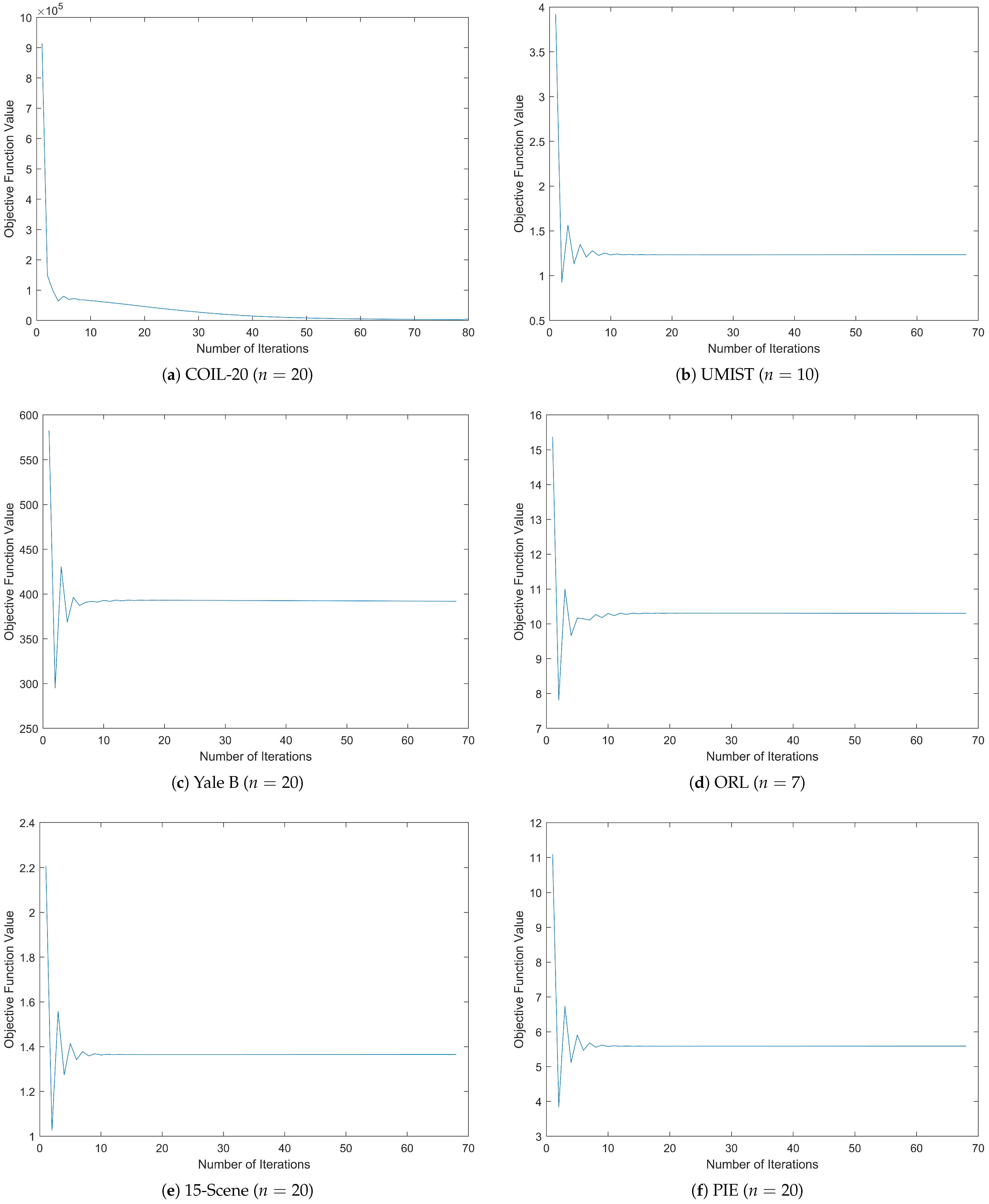
4. Convergence and Complexity

This section proves the convergence of the RDNSLRP model and discusses the computational complexity theoretically.

4.1. Convergence

The objective function of RDNSLRP (11) is a non-convex constrained optimization problem, and its convergence is difficult to be proved directly. However, by employing the ALM–ADM strategy, the whole algorithm is divided into six sub-problems aimed at updating four variables ($\mathbf{P}$, $\mathbf{Z}$, $\mathbf{S}$ and $\mathbf{J}$) and two Lagrange multipliers (${\mathbf{Y}}_1$ and ${\mathbf{Y}}_2$). Therefore, the convergence of overall objective function (11) can be derived by proving the convergence of all the sub-problems.

Firstly, the method for updating $\mathbf{Z}$ by objective function (19) is obtained by the singular value thresholding (SVT) method, and its convergence has been proved in [35]. Secondly, it can be proved through the auxiliary function strategy [37] that objective function (25) monotonically decreases and is lower-bounded, so the sub-problem for updating $\mathbf{S}$ is convergent according to the monotone bounded theorem. Then, the objective function of updating ${\mathbf{J}}_s$ is an unconstrained optimization problem, and its KKT conditions are as follows:

$$\begin{array}{cc}\hfill & \beta \left(\sum _{j=1}^c{\mathbf{X}}_j^T{\mathbf{PP}}^T{\mathbf{X}}_j{\mathbf{J}}_s-{\mathbf{X}}_s^T{\mathbf{PP}}^T{\mathbf{X}}_s\right)+\mu ({\mathbf{J}}_s-{\mathbf{Z}}_s)-{\left({\mathbf{Y}}_2\right)}_s=\mathbf{0},\hfill \\ \hfill & \mathbf{Z}-\mathbf{J}=\mathbf{0}.\hfill \end{array}$$

(38)

Let ${\mathbf{J}}_s^{+}$ and ${\mathbf{Y}}_2^{+}$ represent the updated values of variables ${\mathbf{J}}_s$ and ${\mathbf{Y}}_2$ after a new iteration, respectively, and the following equations can be obtained based on their respective update formulas:

$$\begin{array}{cc}\hfill & \left(\beta \sum _{j=1}^c{\mathbf{X}}_j^T{\mathbf{PP}}^T{\mathbf{X}}_j+\mu {\mathbf{I}}_{n_s}\right)\left({\mathbf{J}}_s^{+}-{\mathbf{J}}_s\right)=\beta \left({\mathbf{X}}_s^T{\mathbf{PP}}^T{\mathbf{X}}_s-\sum _{j=1}^c{\mathbf{X}}_j^T{\mathbf{PP}}^T{\mathbf{X}}_j{\mathbf{J}}_s\right)\hfill \\ \hfill & +\mu ({\mathbf{Z}}_s-{\mathbf{J}}_s)+{\left({\mathbf{Y}}_2\right)}_s,{\mathbf{Y}}_2^{+}-{\mathbf{Y}}_2=\rho (\mathbf{Z}-\mathbf{J}).\hfill \end{array}$$

(39)

Assuming that both sides of the equations approach zero when the number of iterations t is large enough, the following trend can be obtained:

$$\begin{array}{cc}\hfill & \beta \left({\mathbf{X}}_s^T{\mathbf{PP}}^T{\mathbf{X}}_s-\sum _{j=1}^c{\mathbf{X}}_j^T{\mathbf{PP}}^T{\mathbf{X}}_j{\mathbf{J}}_s\right)+\mu ({\mathbf{Z}}_s-{\mathbf{J}}_s)+{\left({\mathbf{Y}}_2\right)}_s\to \mathbf{0},\hfill \\ \hfill & \mathbf{Z}-\mathbf{J}\to \mathbf{0}.\hfill \end{array}$$

(40)

Therefore, according to (38), if the variable ${\mathbf{J}}_s$ converges to a fixed point, i.e., ${\mathbf{J}}_s^{+}-{\mathbf{J}}_s\to \mathbf{0}$ then the fixed point satisfies the KKT condition, thereby proving the convergence of the updating rules of ${\mathbf{J}}_s$. The convergence of updating Lagrange multipliers ${\mathbf{Y}}_1$ and ${\mathbf{Y}}_2$ can also be proved by a similar analytical method. Finally, for the sub-problem of updating $\mathbf{P}$, the objective function (14) is bounded, due to the existence of orthogonal and non-negative constraints. In conclusion, since the objective functions of the six sub-optimization problems are all convergent, the total convergence of the objective function of the RDNSLRP method can be derived.

4.2. Complexity

This subsection discusses the computational complexity of Algorithm 1, which mainly consists of two parts, namely, time complexity and space complexity.

For time complexity, according to Algorithm 1, the optimization process of solving problem (13) can be divided into several independent sub-problems, among which updating variables $\mathbf{P}$, $\mathbf{Z}$, $\mathbf{S}$ and $\mathbf{J}$ are time-consuming. When updating the projection matrix $\mathbf{P}$, the most time-consuming part is the eigenvalue decomposition of temporary variable $\mathbf{H}$, whose time complexity is $O\left(m^3\right)$. Therefore, the time complexity of updating $\mathbf{P}$ is about $O\left(m^3\right)$. Similarly, updating $\mathbf{Z}$ involves the singular-value decomposition of the temporary variable $\mathbf{W}$, whose time complexity is $O\left(n^3\right)$, so the time complexity is nearly $O\left(n^3\right)$. The construction process of both matrix $\mathbf{A}$ and $\mathbf{S}$ costs $O\left(n^2\right)$, from which it can be inferred that the time complexity of updating $\mathbf{S}$ is $O\left(2n^2\right)$. It should be noted that since the construction of matrix $\mathbf{A}$ involves matrix multiplication the time consumption of this step is greater than that of updating $\mathbf{S}$ during iterations. The process of updating $\mathbf{J}$ can be divided into two parts. The first part is to calculate every sub-matrix ${\mathbf{J}}_s$, whose time complexity is about $O\left(2n_s^{2.373}\right)$ [38], and the second part is to merge all sub-matrices to a block-diagonal matrix $\mathbf{J}$ with the total time complexity of $O\left(c\right)$. Therefore, the time complexity of updating $\mathbf{J}$ is around $O\left(c(2n_s^{2.373}+1)\right)$. In summary, the total time complexity of RDNSLRP approximates $O\left(t(m^3+n^3+2n^2+c(2n_s^{2.373}+1))\right)$ if the number of iterations t is given. In our experiment, the maximum number of iterations was set to 100 to avoid overfitting and reduce time consumption.

For space complexity, due to the introduction of other temporary variables in the iterative process of Algorithm 1, its space complexity depends on the dimensions of the block variables and the introduced temporary variables. When updating $\mathbf{P}\in {\mathbb{R}}^{m\times d}$, three temporary variables are introduced, i.e., ${\mathbf{B}}_1\in {\mathbb{R}}^{m\times n_s}$, ${\mathbf{B}}_2\in {\mathbb{R}}^{m\times n_s}$ and $\mathbf{H}\in {\mathbb{R}}^{m\times m}$. Therefore, the space complexity of updating $\mathbf{P}$ is $O(2m{n}_s+m^2+md)$. Updating $\mathbf{Z}\in {\mathbb{R}}^{n\times n}$ involves the calculation of r positive singular values and the introduction of temporary variables $\mathbf{M}\in {\mathbb{R}}^{2n\times n}$, $\mathbf{N}\in {\mathbb{R}}^{2n\times n}$, $\mathbf{B}\in {\mathbb{R}}^{n\times n}$, $\mathbf{U}\in {\mathbb{R}}^{n\times r}$ and $\mathbf{V}\in {\mathbb{R}}^{n\times r}$, which leads to the total space complexity of $O(6n^2+2nr+r)$. Updating $\mathbf{S}\in {\mathbb{R}}^{n\times n}$ involves constructing temporary variables $\mathbf{A}\in {\mathbb{R}}^{n\times n}$ and $\mathbf{Q}\in {\mathbb{R}}^{n\times n}$, and two other temporary variables, namely, ${\mathbf{Q}}^{+}\in {\mathbb{R}}^{n\times n}$ and ${\mathbf{Q}}^{-}\in {\mathbb{R}}^{n\times n}$, need to be calculated, respectively, based on $\mathbf{Q}$, so its space complexity is $O\left(5n^2\right)$. Updating $\mathbf{J}\in {\mathbb{R}}^{n\times n}$ does not entail the introduction of temporary variables and merely occupies a space complexity of $O\left(n^2\right)$. For updating ${\mathbf{Y}}_1\in {\mathbb{R}}^{n\times n}$, ${\mathbf{Y}}_2\in {\mathbb{R}}^{n\times n}$ and $\rho$, no temporary variable is introduced, so their space complexities are $O\left(n^2\right)$, $O\left(n^2\right)$ and $O\left(1\right)$, respectively. In summary, the maximum space complexity of RDNSLRP is $O(14n^2+m^2+2m{n}_s+md+2nr+r+1)$. However, in practical applications, the space consumption can be reduced through pre-computation (such as $\eta$ in updating $\mathbf{Z}$), re-usage of temporary variables and other methods, thereby reducing the space complexity of the proposed algorithm.

5. Experiments and Analyses

This section focuses on analyzing the essential aspects of the RDNSLRP method in the context of unsupervised feature extraction. Image recognition performances on several publicly available data sets were evaluated on RDNSLRP and some state-of-the-art relevant unsupervised feature extraction methods.

5.1. Data Sets and Experimental Settings

In the subsequent experiments, six benchmark data sets were used to evaluate the image recognition performance of RDNSLRP and compared with other state-of-the-art relevant methods, including two small-size face image data sets (ORL [39], UMIST [40]), a middle-size face image data set (Yale B [41,42]), a large-size face image data set (PIE [43]), an object data set (COIL-20 [44]), a realistic scenery image data set (15-Scene [45]) and a large-size handwritten digit data set (MNIST [46]). The detailed characteristics of all the benchmark data sets are listed in

Table 1. Details of all data sets.

Data Set	Samples	Dimensions	Classes
ORL	400	1024	40
UMIST	575	644	20
Yale B	2414	1024	38
PIE	11,554	1024	68
COIL-20	1440	1024	20
15-Scene	4485	3000	15
MNIST	70,000	784	10

:

In addition, the state-of-the-art unsupervised feature extraction methods that were relevant to the proposed method included latent low-rank representation (LatLRR) [10], double low-rank representation (DLRR) [11], low-rank embedding (LRE) [47], low-rank preserving projections (LRPP) [23], low-rank preserving projection via graph regularized representation (LRPP_GRR) [25], the discriminative feature extraction method based on sparse and low-rank representation (DFE) [21], joint low-rank representation and spectral regression learning (JLRSL) [48] and joint local preserving and low-rank representation with non-negative and symmetric constraint (JLPLRNS) [7]. For the RDNSLRP method, the value ranges of the two parameters were given, and all the parameter combinations within these value ranges were enumerated to find the parameter combination that could achieve the optimal result. For all the comparison methods, the parameter combinations were adjusted according to the parameter analyses suggested in their respective original papers. If the parameter sensitivity analyses in the original papers were unavailable or failed to yield the optimal experimental result, the same approach as in RDNSLRP was adopted to search for the optimal parameter combination. In addition, all algorithms were repeated 10 times on each data set and the average recognition accuracies and standard derivations were taken, to ensure the fairness and reliability of the experimental results, unless otherwise specified.

5.2. Experiments on Image Recognition

In order to verify the image recognition performance of the RDNSLRP method, the data sets were divided into training and testing sets. For each data set, n images were randomly selected from each class as training sets, and other images were applied for testing. For the ORL data set, $n=3,5,7$. For the UMIST data set, $n=5,8,10$. For the Yale B, PIE, COIL-20 and 15-Scene data sets, $n=10,15,20$. For the MNIST data set, $n=10,20,30,40,50$. In addition, feature dimension d was set to be the maximum of 400 to ensure the best recognition accuracy for all the methods and to reduce time consumption. The average image recognition accuracies and standard derivations of all the algorithms on these data sets are shown in

Table 2. Average recognition accuracies (%) of different methods on ORL and UMIST data sets.

Data Sets	ORL			UMIST
n	3	5	7	5	8	10
LatLRR	$75.464\pm 2.62$	$86.550\pm 2.19$	$91.583\pm 2.40$	$81.582\pm 1.50$	$91.205\pm 1.97$	$94.261\pm 2.31$
DLRR	$67.857\pm 1.97$	$80.650\pm 2.48$	$88.167\pm 2.89$	$77.768\pm 2.58$	$89.595\pm 1.73$	$92.907\pm 1.67$
LRE	$76.786\pm 2.21$	$86.750\pm 2.18$	$91.333\pm 1.81$	$81.347\pm 2.54$	$90.024\pm 1.52$	$94.320\pm 1.38$
LRPP	$75.393\pm 2.37$	$85.750\pm 1.57$	$90.833\pm 0.96$	$79.747\pm 2.52$	$90.409\pm 2.35$	$94.406\pm 1.24$
LRPP_GRR	$74.539\pm 2.61$	$83.650\pm 1.83$	$87.250\pm 1.67$	$79.726\pm 2.46$	$87.735\pm 1.98$	$93.307\pm 1.56$
DFE	$\underline{84.998}\pm 2.55$	$\underline{91.650}\pm 1.49$	$93.500\pm 2.11$	$\underline{84.147}\pm 1.72$	$\underline{92.964}\pm 1.61$	$\underline{96.267}\pm 1.34$
JLRSL	$80.491\pm 2.48$	$89.100\pm 1.93$	$\underline{94.167}\pm 1.92$	$84.014\pm 1.89$	$88.787\pm 1.66$	$92.907\pm 1.39$
JLPLRNS	$73.714\pm 2.25$	$85.050\pm 2.73$	$89.697\pm 1.59$	$73.748\pm 2.43$	$86.458\pm 1.73$	$91.467\pm 2.26$
RDNSLRP	$\mathbf{88.550}\pm 2.17$	$\mathbf{96.450}\pm 1.01$	$\mathbf{98.250}\pm 0.92$	$\mathbf{88.694}\pm 1.93$	$\mathbf{96.410}\pm 1.34$	$\mathbf{97.402}\pm 1.45$

,

Table 3. Average recognition accuracies (%) of different methods on Yale B and PIE data sets.

Data Sets	Yale B			PIE
n	10	15	20	10	15	20
LatLRR	$47.021\pm 1.02$	$55.655\pm 1.12$	$62.273\pm 1.13$	$42.744\pm 0.71$	$52.488\pm 0.51$	$60.154\pm 0.72$
DLRR	$33.742\pm 3.80$	$45.266\pm 3.56$	$51.369\pm 2.71$	$34.186\pm 1.39$	$46.002\pm 2.31$	$54.915\pm 1.40$
LRE	$66.763\pm 1.79$	$79.136\pm 1.50$	$83.661\pm 0.96$	$63.229\pm 1.31$	$75.461\pm 1.84$	$80.646\pm 0.92$
LRPP	$72.271\pm 1.44$	$80.862\pm 1.38$	$84.460\pm 1.53$	$68.420\pm 1.56$	$77.709\pm 1.96$	$82.859\pm 1.32$
LRPP_GRR	$83.508\pm 0.79$	$\underline{88.671}\pm 0.79$	$\underline{91.391}\pm 0.47$	$\underline{75.801}\pm 0.63$	$\underline{83.237}\pm 0.40$	$\underline{87.922}\pm 0.73$
DFE	$78.574\pm 1.35$	$86.604\pm 1.13$	$90.091\pm 0.57$	$72.548\pm 1.22$	$81.988\pm 0.87$	$86.841\pm 0.69$
JLRSL	$61.854\pm 3.25$	$80.217\pm 1.26$	$89.956\pm 0.45$	$74.055\pm 1.13$	$81.857\pm 0.96$	$85.983\pm 0.70$
JLPLRNS	$\underline{84.491}\pm 0.76$	$88.471\pm 0.47$	$90.103\pm 0.39$	$74.439\pm 0.74$	$81.292\pm 0.52$	$85.847\pm 0.64$
RDNSLRP	$\mathbf{85.639}\pm 1.10$	$\mathbf{89.468}\pm 1.13$	$\mathbf{91.783}\pm 0.77$	$\mathbf{84.357}\pm 0.90$	$\mathbf{87.248}\pm 0.84$	$\mathbf{89.256}\pm 0.60$

,

Table 4. Average recognition accuracies (%) of different methods on COIL-20 and 15-Scene data sets.

Data Sets	COIL-20			15-Scene
n	10	15	20	10	15	20
LatLRR	$88.353\pm 1.48$	$92.088\pm 1.02$	$93.462\pm 0.77$	$85.764\pm 1.05$	$88.197\pm 1.01$	$89.536\pm 0.72$
DLRR	$88.737\pm 1.36$	$92.141\pm 0.84$	$93.365\pm 0.91$	$85.648\pm 1.16$	$88.211\pm 0.77$	$89.327\pm 0.86$
LRE	$89.671\pm 1.23$	$92.102\pm 0.93$	$93.777\pm 0.65$	$\underline{86.058}\pm 0.38$	$88.005\pm 0.74$	$89.458\pm 0.66$
LRPP	$89.637\pm 1.44$	$93.346\pm 1.13$	$94.261\pm 0.84$	$84.875\pm 1.07$	$87.809\pm 0.97$	$89.022\pm 0.88$
LRPP_GRR	$89.508\pm 1.85$	$\mathbf{94.044}\pm 0.84$	$\mathbf{96.612}\pm 0.62$	$85.728\pm 1.47$	$87.042\pm 0.78$	$89.460\pm 0.52$
DFE	$\underline{90.347}\pm 1.01$	$\underline{93.675}\pm 0.92$	$\underline{95.192}\pm 1.17$	$85.879\pm 1.10$	$87.962\pm 0.81$	$\underline{90.024}\pm 0.94$
JLRSL	$88.638\pm 1.38$	$92.263\pm 0.96$	$94.029\pm 0.58$	$84.539\pm 0.81$	$\underline{88.283}\pm 0.64$	$89.851\pm 0.66$
JLPLRNS	$83.105\pm 1.60$	$91.474\pm 1.00$	$94.519\pm 0.64$	$80.295\pm 1.24$	$83.576\pm 0.80$	$85.448\pm 1.35$
RDNSLRP	$\mathbf{90.605}\pm 1.21$	$92.816\pm 0.63$	$94.671\pm 0.93$	$\mathbf{87.025}\pm 0.86$	$\mathbf{89.685}\pm 0.90$	$\mathbf{91.238}\pm 0.85$

and

Table 5. Average recognition accuracies (%) of different methods on MNIST data set.

Data Sets	MNIST
n	10	20	30	40	50
LatLRR	$74.114\pm 0.70$	$80.679\pm 1.21$	$83.428\pm 0.72$	$85.518\pm 0.67$	$\mathbf{87.039}\pm 0.68$
DLRR	$74.067\pm 1.08$	$\underline{81.682}\pm 0.86$	$83.445\pm 0.79$	$85.622\pm 0.47$	$\underline{86.873}\pm 0.61$
LRE	$\underline{74.677}\pm 1.02$	$80.901\pm 1.58$	$83.663\pm 0.64$	$\mathbf{85.844}\pm 0.70$	$85.412\pm 0.75$
LRPP	$73.643\pm 1.84$	$80.873\pm 1.24$	$\underline{83.690}\pm 0.93$	$\underline{85.734}\pm 0.28$	$85.828\pm 0.59$
LRPP_GRR	$64.139\pm 1.59$	$69.091\pm 1.89$	$71.765\pm 1.02$	$73.431\pm 0.83$	$75.188\pm 0.75$
DFE	$74.012\pm 0.99$	$79.525\pm 1.01$	$82.001\pm 0.79$	$83.251\pm 0.66$	$83.720\pm 0.53$
JLRSL	$60.496\pm 2.08$	$68.292\pm 1.73$	$72.358\pm 1.85$	$75.019\pm 1.18$	$76.204\pm 1.03$
JLPLRNS	$65.497\pm 2.10$	$71.563\pm 1.44$	$78.236\pm 1.08$	$80.224\pm 0.81$	$80.522\pm 0.71$
RDNSLRP	$\mathbf{75.119}\pm 1.31$	$\mathbf{81.766}\pm 0.95$	$\mathbf{83.750}\pm 1.14$	$85.062\pm 0.89$	$85.668\pm 0.67$

, respectively, where the best and second-best results are, respectively, shown in bold and underlined.

It can be observed from these tables that the RDNSLRP method outperformed the compared methods and achieved the best image recognition accuracies on five data sets. In addition, RDNSLRP demonstrated superior image recognition accuracies when the sizes of the training sets n were small, and it remained competitive as n increased. For example, the image recognition accuracy of RDNSLRP exceeded the sub-optimal values by 8.556%, 4.011% and 1.334%, respectively, on the PIE data set. The experimental results indicate that RDNSLRP can effectively address image recognition tasks, particularly on training sets with smaller sizes.

The main reasons why the RDNSLRP method can achieve the best image recognition performance are as follows. Firstly, by imposing non-negative and symmetric constraints, the coefficient matrix $\mathbf{Z}$ obtained through RDNSLRP has strong interpretability and better structural properties, which are utilized to promote the learning effort of projection matrix $\mathbf{P}$. Therefore, compared with methods that do not constrain matrix $\mathbf{Z}$ (such as LRE, LRPP, JLRSL), RDNSLRP demonstrates significant advantages. Secondly, RDNSLRP introduces a graph-based manifold learning method to low-rank representation, enabling the graph matrix $\mathbf{Z}$ to extract both global and intrinsic features, while preserving the more geometric structures of the original data. Compared to methods such as LatLRR, DLRR—which directly employs a low-rank projection matrix $\mathbf{L}$—and DFE, which utilizes sparse representation to extract intrinsic features, RDNSLRP can fully explore the intrinsic structure of training samples, resulting in higher image recognition accuracies on data sets that contain more complex intrinsic information (such as Yale B and PIE). Finally, the discriminant term (9) further increases the inter-class divergence and decreases intra-class divergence by simultaneously reinforcing the block-diagonal regions of the graph matrix $\mathbf{Z}$ and diminishing the influence of other regions during the learning process. Additionally, the influence of the reconstruction error of the same sample in low-dimensional subspace is considered, so that the influence of noise and outliers is mitigated. Therefore, RDNSLRP has a better image recognition effect than JLPLRNS. For the above reasons, RDNSLRP is more discriminative than other methods in the task of feature extraction, leading to overall better image recognition performance.

5.3. Experiments on Noisy Data Sets

In order to evaluate the robustness of the RDNSLRP method against noise, various densities of Gaussian noise were introduced. Taking the UMIST ($n=10$) and PIE ($n=20$) data sets as examples, Gaussian noise with densities ranging from 10% to 40% were added to all the images on both data sets. Figure 3 illustrates the changes in the image recognition accuracy of the different methods as the density of Gaussian noise increased. Additionally, in order to provide a more intuitive demonstration of each method’s robustness to noise, the image recognition accuracies on the noisy data sets and their relative reductions compared to those on noise-free data sets are presented in

Table 6. Image recognition accuracies (%) and reduction on noise-corrupted UMIST data set.

Noise Density	10	20	30	40
LatLRR	94.133 (−0.267)	93.6 (−0.800)	94.133 (−0.267)	94.133 (−0.267)
DLRR	93.867 (−0.266)	93.6 (−0.533)	94.133 (−0.000)	92.533 (−1.600)
LRE	94.133 (−0.000)	93.6 (−0.533)	94.133 (−0.000)	92.533 (−1.600)
LRPP	94.667 (−0.166)	94.4 (−0.433)	93.333 (−1.500)	93.333 (−1.500)
LRPP_GRR	94.133 (−0.267)	93.533 (−0.867)	92.0 (−2.400)	88.8 (−5.600)
DFE	96.8 (−0.533)	96.267 (−1.066)	95.467 (−1.866)	94.4 (−2.933)
JLRSL	92.8 (−0.107)	92.533 (−0.374)	92.0 (−0.907)	91.333 (−1.574)
JLPLRNS	90.667 (−0.666)	88.8 (−2.533)	87.2 (−4.133)	86.667 (−4.666)
RDNSLRP	97.867 (−0.000)	97.6 (−0.267)	96.267 (−1.600)	95.2 (−2.667)

and

Table 7. Image recognition accuracies (%) and reduction on noise-corrupted PIE data set.

Noise Density	10	20	30	40
LatLRR	59.692 (−2.011)	58.878 (−2.825)	58.878 (−2.825)	58.211 (−3.492)
DLRR	54.101 (−2.550)	52.266 (−4.385)	51.766 (−4.885)	50.579 (−6.072)
LRE	81.783 (−2.076)	80.742 (−3.117)	77.969 (−5.890)	71.130 (−11.729)
LRPP	80.742 (−2.495)	77.652 (−5.585)	75.247 (−7.990)	71.580 (−11.657)
LRPP_GRR	86.463 (−1.059)	84.344 (−3.178)	82.715 (−4.807)	77.183 (−10.339)
DFE	84.265 (−1.599)	83.0 (−2.864)	80.636 (−5.228)	78.693 (−7.171)
JLRSL	84.409 (−1.484)	80.945 (−4.948)	79.547 (−6.346)	77.886 (−8.007)
JLPLRNS	82.232 (−2.141)	78.458 (−5.915)	76.720 (−7.653)	73.465 (−10.908)
RDNSLRP	87.589 (−0.917)	85.922 (−2.584)	83.744 (−4.372)	82.459 (−6.047)

, respectively, where the best results are highlighted in bold and the second-best results are underlined.

As shown in Figure 3 and the two tables, the image recognition accuracy of all the methods generally decreased as the noise density increased. The RDNSLRP method achieved the highest accuracies on both data sets while maintaining the lowest or second-lowest reduction in most cases. In particular, the RDNSLRP method achieved the smallest reduction on both data sets when the noise density was relatively low (less than 20%). In addition, although the reduction in the image recognition accuracy of RDNSLRP was not the lowest on the UMIST data set, it was still competitive compared with other methods. The experimental results demonstrate that the RDNSLRP method shows greater robustness against noise than other comparison methods, overall.

5.4. Experiments on Dimensional Reduction

To further investigate the image recognition performance under various feature dimensions, data sets PIE ($n=20$), ORL ($n=7$), 15-Scene ($n=20$) and UMIST ($n=10$) were taken as examples to evaluate the image recognition accuracies of RDNSLRP and other comparison methods based on dimensionality reduction. Since the projection matrices learned by LatLRR and DLRR retain the same dimensions as the original data set, these methods do not employ dimensional reduction techniques and are not discussed here. For the larger data sets, PIE and 15-Scene, the variation range of the feature dimension was set to $d\in (0,400]$. For the ORL and UMIST data sets, the variation range was set to $d\in (0,200]$. The correlations between image recognition accuracy and feature dimension are illustrated in Figure 4:

According to Figure 4, RDNSLRP demonstrated superior image recognition accuracy across most feature dimensions compared to the other methods, and it reached the peak value at lower feature dimensions. For example, RDNSLRP reached the optimal accuracies at the feature dimensions of 30, 20, 10 on the ORL, 15-Scene and UMIST data sets, respectively. Although at low feature dimensions, the image recognition accuracy of RDNSLRP on the PIE data set was slightly lower than that of some comparison methods, RDNSLRP remained highly competitive overall. In addition, as the feature dimension increased, the image recognition curves for RDNSLRP across all the data sets were smoother compared to the other methods. While some comparison methods performed better than RDNSLRP on individual data sets at certain feature dimensions, only the RDNSLRP method consistently achieved favorable results across all data sets. Therefore, the RDNSLRP method was not only less affected by the change of feature dimension in image recognition tasks, but also performed stably on different data sets.

5.5. Comparison with Deep Learning Methods

In recent years, deep learning methods have attained remarkable achievements and have emerged as the mainstream in feature extraction. To this end, four classical deep learning-based feature extraction methods, AlexNet [49], LeNet-5 [50], VGG-16 [51] and Xception [52], were introduced as comparison methods for the performance of image recognition. In addition, PIE ($n=10$), Extended Yale B ($n=10$) and UMIST ($n=10$) were taken as examples. Firstly, pre-training was carried out for these four networks, and then the data were input to four pre-trained deep networks to proceed with feature extraction. The image recognition accuracies obtained by RDNSLRP and the deep learning methods are presented in

Table 8. Comparison of image recognition accuracy (%) between RDNSLRP and deep learning methods.

Data Sets	PIE	Yale B	UMIST
AlexNet	$\underline{82.961}$	$76.261$	$94.461$
LeNet-5	$81.057$	$74.620$	$92.133$
VGG-16	$81.745$	$\underline{84.474}$	$\underline{96.750}$
Xception	$79.655$	$80.793$	$94.225$
RDNSLRP	$\mathbf{84.357}$	$\mathbf{85.639}$	$\mathbf{97.402}$

, where the best and the second-best results are marked in bold and underlined, respectively. It can be observed from Table 8 that the proposed method outperformed these deep learning methods, in terms of image recognition performance.

5.6. Analysis of Convergence

In Section 4.1, the convergence of the objective function of RDNSLRP was proved theoretically. For this subsection, the changes of the objective function values in model (11) with the increase of iteration times were studied on specific data sets, and their convergence was verified experimentally. For all the data sets, except MNIST, n images from each class were randomly selected as training sets, and other images were used for testing. Then, the variation of the objective function value of (11) with the increase in the iteration times of Algorithm 1 was observed on each data set. Specifically, the updated block variables were substituted into objective function (11) to obtain the corresponding objective function value for each iteration. Figure 5 reveals the curves of the objective function values of (11) on all the data sets as the number of iterations increased.

It can be observed from the figures that the objective function value of (11) dropped sharply during the first iteration and fluctuated in the subsequent few iterations. Then, as the number of iterations increased, the amplitude of these fluctuations gradually decreased and became stable after about 10 to 20 iterations. In addition, (11) reached the convergence condition after 80 iterations on the COIL-20 data set and after 69 iterations on all the other data sets. Similar trends were also observed when n took other values on all the data sets, which indicates that the RDNSLRP model has good convergence and that the maximum number of iterations can be set as a relatively small value in practical applications.

5.7. Analysis of Time Consumption

In Section 4.2, the time complexity of Algorithm 1 was analyzed in theory. In this subsection, the time consumed in the learning process by all the algorithms and the corresponding number of iterations required to reach the convergence conditions are given, through experiments on four data sets, UMIST ($n=10$), COIL-20 ($n=20$), 15-Scene ($n=20$) and PIE ($n=20$). In addition, it should be noted that the maximum number of iterations for the LRPP and JLPLRNS methods was set to 100 to prevent overfitting and computational errors (such as NaN or infinite values).

Table 9. Time consumption and the number of iterations (in brackets) on four data sets.

Data Sets	UMIST	COIL-20	15-Scene	PIE
LatLRR	8.701 (329)	52.588 (284)	706.72 (197)	179.65 (331)
DLRR	13.670 (250)	31.191 (226)	811.08 (225)	114.73 (234)
LRE	5.693 (208)	14.085 (210)	34.029 (289)	108.21 (300)
LRPP	29.151 (100)	206.28 (100)	392.94 (100)	1710.2 (100)
LRPP_GRR	11.861 (283)	35.379 (300)	96.226 (257)	116.27 (225)
DFE	2.538 (80)	7.696 (80)	69.493 (80)	53.726 (80)
JLRSL	6.116 (179)	25.445 (199)	92.161 (229)	684.88 (247)
JLPLRNS	1.644 (100)	5.163 (100)	14.632 (100)	39.176 (100)
RDNSLRP	23.068 (69)	108.74 (71)	301.71 (69)	1017.9 (69)

shows the time consumption and number of iterations of each method in the image recognition experiment, with the shortest and second-shortest time consumption marked in bold and underlined, respectively. The lowest and second-lowest number of iterations required are also respectively marked in bold and underlined. It can be seen from the table that, although Algorithm 1 required the least number of iterations among all the algorithms, it consumed a relatively high amount of time to reach its convergence conditions. This was mainly due to the involved time-consuming operations, such as eigenvalue decomposition, singular value decomposition and construction of large-size matrices. Fortunately, as is summarized in Section 5.5, by setting the maximum number of iterations at a relatively small value, the optimal image recognition result could be obtained in a shorter time consumption.

5.8. Analysis of Parameter Sensitivity

There are two regularization parameters $\alpha$ and $\beta$ in model (10), which are used for balancing low-rank terms and discriminant terms, respectively. For this section, we employed the control variates method to analyze their respective influence on image recognition accuracy. Specifically, one parameter was changed within a specified range while another parameter was fixed. Then, the variation trend of the image recognition accuracy of RDNSLRP could be observed and analyzed on the UMIST ($n=8$), Yale B ($n=15$), ORL ($n=5$), 15-Scene ($n=20$), COIL-20 ($n=15$) and MNIST ($n=10$) data sets. Meanwhile, the values of parameters $\alpha$ and $\beta$ were both chosen in the candidate set of $\{{10}^{-4},{10}^{-3},{10}^{-2},{10}^{-1},1,10,100\}$ for the UMIST, Yale B, ORL, COIL-20 and 15-Scene data sets, and in the set of $\{{10}^{-3},{10}^{-2},{10}^{-1},1,10,100,1000\}$ for the MNIST data set. The influence of parameter combination $(\alpha ,\beta )$ on the image recognition accuracy of RDNSLRP on these data sets is shown in Figure 6. It should be noted that the different colors in the subfigures are the default colors for matlab and are only used to distinguish experimental results obtained by different values of $\beta$.

As can be seen from the first four subfigures of Figure 6, when parameter $\alpha$ was fixed the image recognition accuracy remained stable when the value of $\beta$ was small and decreased as the value of $\beta$ increased. Similarly, when $\beta$ was fixed, the change of image recognition accuracy was not obvious when $\alpha$ was small, and an obvious decline occurred when $\alpha >1$ on all data sets. It can be inferred from the experimental results that in a certain range of values both parameters have little influence on the image recognition performance of RDNSLRP, especially when both $\alpha$ and $\beta$ are set to relatively small values. Otherwise, when the value of one of the parameters is large, the image recognition performance of RDNSLRP may deteriorate. It is necessary to note that the images in the UMIST, Yale B, ORL and 15-Scene data sets corresponding to these subfigures all possess a considerable amount of intrinsic structures. In other words, there is correlative information among different features of the same image. Therefore, when the parameters $\alpha$ and $\beta$ are chosen to be relatively small, the weight of the adaptive graph regularization term in the model increases, which helps increase the extraction of the intrinsic features of the original data. Conversely, when one of the parameter values is chosen to be very large, it might result in the reduction of the image recognition performance, due to the inability to effectively extract the intrinsic features. Therefore, in practical applications, both parameters should be taken to a smaller value to ensure the feature extraction performance on the data sets with an amount of intrinsic features.

The other two subfigures showed completely different parameter sensitivity patterns. As illustrated in the last two subfigures of Figure 6, the variation of the image recognition accuracy of RDNSLRP on the COIL-20 and MNIST data sets with the increase in the value of $\alpha$ was not obvious when $\beta$ was fixed. However, when the value of $\alpha$ was fixed the image recognition accuracy initially decreased and then increased with the increase in the value of $\beta$, and it was higher when $\beta$ took a larger value, demonstrating that RDNSLRP is not sensitive to parameter $\alpha$ but is sensitive to $\beta$ on these data sets. This indicates that on data sets that mainly rely on global features for image recognition, such as COIL-20 and MNIST, parameter $\beta$ should be preferably selected to be relatively large values, enabling larger weights of the low-rank term and the discriminant term in the proposed model, thereby facilitating the extraction of the global features of the data. Therefore, in practical applications, parameter $\beta$ should be set to a relatively large value on data sets with more global structures and less intrinsic structures. In addition, in order to achieve the optimal image recognition performance on different data sets it is recommended to employ other techniques, such as grid search, to rapidly obtain the optimal parameter combination.

6. Discussion

In the previous sections, RDNSLRP was proposed and its usability and practicability were verified through experiments. However, RDNSLRP is not a flawless model. In this section, existing and potential limitations are discussed and future works are also proposed, with respect to these limitations.

6.1. Limitations

This subsection primarily discusses some limitations of the RDNSLRP method. Some of these limitations are shared by all traditional learning methods while others are specific to RDNSLRP itself. Furthermore, potential improvement approaches for each limitation are also discussed, for subsequent researchers to conduct studies and make enhancements.

• It can be observed from the tables in Section 5.2 that when n is set to be a relatively large value, the image recognition accuracy of RDNSLRP on COIL-20 and MNIST is inferior to that of some other methods. Considering that these two data sets are dominated by global features, this might be attributable to the possibility that RDNSLRP does not adopt measures to enhance the extraction of the global structure information of the data samples in the original subspace. AGE_PPL [27] provides a good example of simultaneously considering the intrinsic and global structural information in the original space. Therefore, in addition to considering the intrinsic relationships among samples in the projected subspace, it is also necessary to maintain the global structure in the original space, to obtain more comprehensive structural information about the sample images.
• According to the analysis in Section 5.7, the time consumption of RDNSLRP escalates rapidly when the training set grows larger. Decreasing the time complexity via certain mathematical approaches might further reduce the time consumption.
• However, the arduous challenge of traditional machine learning methods based on low-rank representation in dealing with ultra large-scale training sets (e.g., the CelebA data set [53]) still exists, which cannot be simply resolved through mathematical approaches. It is necessary to consider integrating these methods with some popular data processing strategies, including but not limited to deep learning and distributed parallel computing, to effectively boost the speed of data processing and address other potential problems.
• Furthermore, there exist issues such as the incapability of handling highly non-linear data (e.g., the PubFig data set [54]) and extremely small sample data (e.g., the LFW data set [55]). Considering the increasing complexity of data in real-world applications, such problems might necessitate improvements to the low-rank representation method for resolution.

6.2. Future Works

In this subsection, future research works, in light of the RDNSLRP model’s limitations, are presented. Firstly, continuous research on and improvement of RDNSLRP will be pursued, with regard to the limitations in maintaining and extracting global structures, as well as time complexity. Secondly, in response to the challenges posed by traditional machine learning methods when handling ultra-large-scale and complex data sets, the combination of RDNSLRP with deep learning methods, such as neural networks, will be contemplated, and generalization experiments will be carried out. Furthermore, how to incorporate the fundamental concepts of low-rank representation and RDNSLRP into deep learning and investigate novel feature extraction methods is worthy of future study.

7. Conclusions

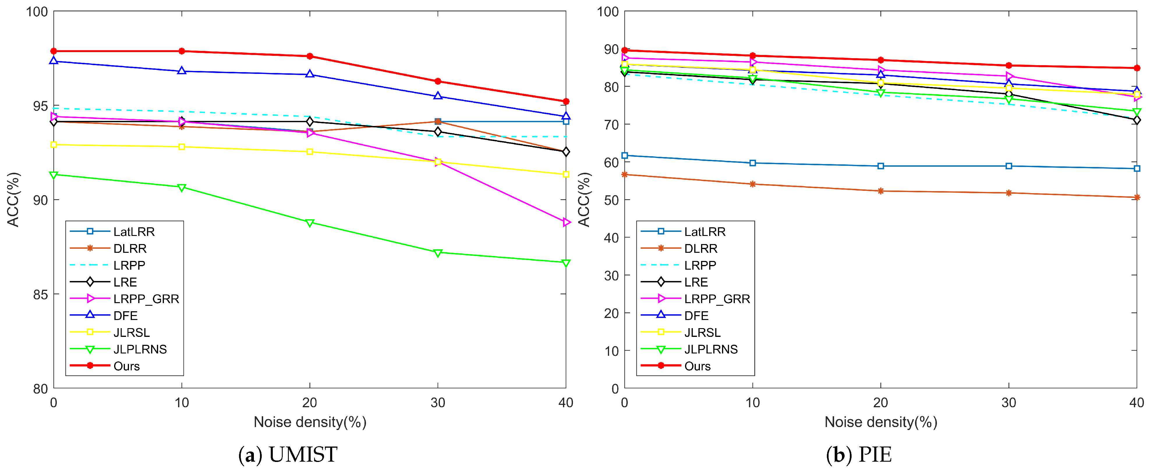
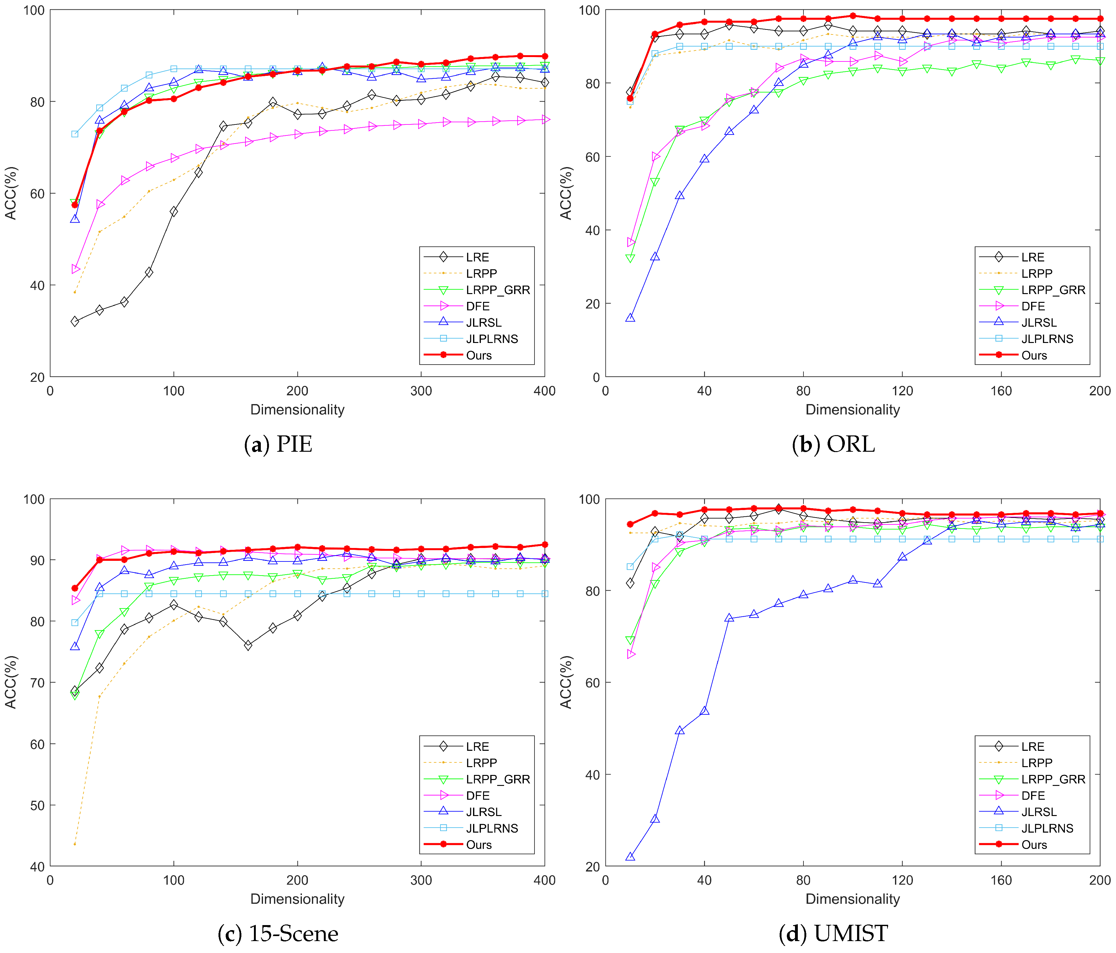
In this paper, a novel model, RDNSLRP, has been proposed for unsupervised feature extraction. A low-rank coefficient matrix with better properties is utilized as the graph matrix for learning the projection matrix, and a discriminant term is introduced to enhance the robustness of the model against noise, as well as the discriminant of extracted features. Therefore, the RDNSLRP model not only makes full use of both the global and the intrinsic structures of the original data, but also effectively separates the impact of noise and outliers; thereby, the performance of feature extraction and image recognition can be improved. A large number of experimental results on several benchmark data sets proved the usability, practicability and performance to be superior to other existing methods, such as in the 8.556% improvement on the PIE data set and the 4.547% improvement on the UMIST data set.

However, RDNSLRP is not flawless, and some limitations exist, including insufficiency in maintaining global structural information and an inability to handle data sets of extremely large scale or complex structure, etc. Therefore, the methods to address these issues, including improving low-rank representation and combining with deep learning methods, are worthy of further study.

References

1. Abdi, H.; Williams, L.J. Principal component analysis. Wires Comput. Stat. 2010, 2, 433–459. [Google Scholar] [CrossRef]
2. Su, T.; Feng, D.; Wang, M.; Chen, M. Dual Discriminative Low-Rank Projection Learning for Robust Image Classification. IEEE Trans. Circuits Syst. Video Technol. 2023, 33, 7708–7722. [Google Scholar] [CrossRef]
3. Liu, G.C.; Lin, Z.C.; Yu, Y. Robust subspace segmentation by low-rank representation. In Proceedings of the 27th International Conference on Machine Learning, Haifa, Isreal, 21–24 June 2010; pp. 663–670. [Google Scholar]
4. Liu, G.C.; Lin, Z.C.; Yan, S.C.; Sun, J.; Yu, Y.; Ma, Y. Robust Recovery of Subspace Structures by Low-Rank Representation. IEEE Trans. Pattern Anal. Mach. Intell. 2013, 35, 171–184. [Google Scholar] [CrossRef] [PubMed]
5. Wang, S.; Wang, H. Unsupervised feature selection via low-rank approximation and structure learning. Knowl.-Based Syst. 2017, 124, 70–79. [Google Scholar] [CrossRef]
6. Zhu, X.; Chen, X. Low-rank nonnegative sparse representation and local preservation-based matrix regression for supervised image feature selection. IET Process 2021, 15, 3021–3036. [Google Scholar] [CrossRef]
7. Xu, Z.; Jiang, L.; Zhu, X.; Chen, X. Non-negative consistency affinity graph learning for unsupervised feature selection and clustering. Eng. Appl. Artif. Intell. 2024, 135, 108784. [Google Scholar] [CrossRef]
8. Kong, Z.; Chang, D.; Fu, Z.; Wang, J.; Wang, Y.M.; Zhao, Y. Projection-preserving block-diagonal low-rank representation for subspace clustering. Neurocomputing 2023, 526, 19–29. [Google Scholar] [CrossRef]
9. Chen, H.; Chen, X.; Tao, H.; Li, Z.; Wang, B. PDRLRR: A novel low-rank representation with projection distance regularization via manifold optimization for clustering. Pattern Recognit. 2024, 149, 110918. [Google Scholar] [CrossRef]
10. Liu, G.C.; Yan, S.C. Latent low-rank representation for subspace segmentation and feature extraction. In Proceedings of the IEEE International Conference on Computer Vision (ICCV), Barcelona, Spain, 6–13 November 2011; pp. 1615–1622. [Google Scholar]
11. Yin, M.; Cai, S.; Gao, J. Robust face recognition via double low-rank matrix recovery for feature extraction. In Proceedings of the IEEE International Conference on Computer Vision (ICCV), Melbourne, Australia, 1–8 December 2013; pp. 3770–3774. [Google Scholar]
12. Song, Y.; Wu, Y. Subspace clustering based on latent low-rank representation with Frobenius norm minimization. Neurocomputing 2018, 275, 2479–2489. [Google Scholar]
13. Fu, Z.; Zhao, Y.; Chang, D.; Zhang, X.; Wang, Y. Double low-rank representation with projection distance penalty for clustering. In Proceedings of the 2021 IEEE/CVF Conference on Computer Vision and Pattern Recognition (CVPR), Nashville, TN, USA, 20–25 June 2021; pp. 5316–5325. [Google Scholar]
14. Qiao, X.; Chen, C.; Wang, W. Efficient subspace clustering and feature extraction via l2,1-norm and l1,2-norm minimization. Neurocomputing 2024, 595, 12813. [Google Scholar] [CrossRef]
15. Fang, X.; Han, N.; Wu, J.; Xu, Y.; Yang, J.; Wong, W.K. Approximate low-rank projection learning for feature extraction. IEEE Trans. Neural Netw. Learn. Syst. 2018, 29, 5228–5241. [Google Scholar] [CrossRef] [PubMed]
16. Lai, Z.; Bao, J.; Kong, H.; Wan, M.; Yang, G. Discriminative low-rank projection for robust subspace learning. Int. J. Mach. Learn. Cybern. 2020, 11, 2247–2260. [Google Scholar] [CrossRef]
17. Ren, Z.; Sun, Q.; Wu, B.; Zhang, X.; Yan, W. Learning latent low-rank and sparse embedding for robust image feature extraction. IEEE Trans. Image Process. 2020, 29, 2094–2107. [Google Scholar] [CrossRef] [PubMed]
18. Wang, J.; Shi, D.; Cheng, D.; Zhang, Y.; Gao, J. LRSR: Low-rank-sparse representation for subspace clustering. Neurocomputing 2016, 214, 1026–1037. [Google Scholar] [CrossRef]
19. Li, J.; Chen, C.; Hou, X.; Wang, R. Laplacian regularized non-negative sparse low-rank representation classification. In Biometric Recognition: Proceedings of the 12th Chinese Conference, CCBR 2017, Shenzhen, China, 28–29 October 2017; Proceedings 12; Springer International Publishing: Berlin/Heidelberg, Germany, 2017; pp. 683–690. [Google Scholar]
20. Meng, M.; Lan, M.; Yu, J.; Wu, J.; Tao, D. Constrained discriminative projection learning for image classification. IEEE Trans. Image Process. 2020, 29, 186–198. [Google Scholar] [CrossRef]
21. Liu, Z.; Ou, W.; Lu, W.; Wang, L. Discriminative feature extraction based on sparse and low-rank representation. Neurocomputing 2019, 362, 129–138. [Google Scholar] [CrossRef]
22. Yu, W.; Teng, X.; Liu, C. Face recognition using discriminant locality preserving projections. Pattern Recognit. Lett. 2009, 30, 1378–1383. [Google Scholar] [CrossRef]
23. Lu, Y.; Lai, Z.; Xu, Y.; Li, X.; Zhang, D.; Yuan, C. Low-rank preserving projections. IEEE Trans. Cybern. 2016, 46, 1900–1913. [Google Scholar] [CrossRef]
24. Wen, J.; Fang, X.; Xu, Y.; Tian, C.; Fei, L. Low-rank representation with adaptive graph regularization. Neural Netw. 2018, 108, 83–96. [Google Scholar] [CrossRef]
25. Wen, J.; Han, N.; Fang, X.; Fei, L.; Yan, K.; Zhan, S. Low-rank preserving projection via graph regularized reconstruction. IEEE Trans. Cybern. 2019, 49, 1279–1291. [Google Scholar] [CrossRef]
26. Ruan, W.; Sun, L. Robust latent discriminative adaptive graph preserving learning for image feature extraction. Knowl.-Based Syst. 2023, 268, 110487. [Google Scholar] [CrossRef]
27. Zhao, S.; Wu, J.; Zhang, B.; Fei, L.; Li, S.; Zhao, P. Adaptive graph embedded preserving projection learning for feature extraction and selection. IEEE Trans. Syst. Man Cybern. Syst. 2023, 53, 1060–1073. [Google Scholar] [CrossRef]
28. Yin, M.; Gao, J.; Lin, Z. Laplacian regularized low-rank representation and its applications. IEEE Trans. Pattern Anal. Mach. Intell. 2016, 38, 504–517. [Google Scholar] [CrossRef]
29. Candes, E.J.; Tao, T. The power of convex relaxation: Near-optimal matrix completion. IEEE Trans. Inf. Theory 2010, 56, 2053–2080. [Google Scholar] [CrossRef]
30. Chen, J.; Mao, H.; Sang, Y.; Yi, Z. Subspace clustering using a symmetric low-rank representation. Knowl.-Based Syst. 2017, 127, 46–57. [Google Scholar] [CrossRef]
31. Xu, J.; An, W.; Zhang, L.; Zhang, D. Sparse, collaborative, or nonnegative representation: Which helps pattern classification? Pattern Recognit. 2019, 88, 679–688. [Google Scholar] [CrossRef]
32. Naseem, I.; Togneri, R.; Bennamoun, M. Linear regression for face recognition. IEEE Trans. Pattern Anal. Mach. Intell. 2010, 32, 2106–2112. [Google Scholar] [CrossRef]
33. Xiang, S.; Nie, F.; Meng, G.; Pan, C.; Zhang, C. Discriminative least squares regression for multiclass classification and feature selection. IEEE Trans. Neural Netw. Learn. Syst. 2012, 23, 1738–1754. [Google Scholar] [CrossRef]
34. Boyd, S.; Parikh, N.; Chu, E.; Pelato, B.; Ecjstein, J. Distributed optimization and statistical learning via the alternating direction method of multipliers. Found. Trends Mach. Learn. 2011, 3, 1–122. [Google Scholar] [CrossRef]
35. Cai, J.F.; Candes, E.J.; Shen, Z. A singular value thresholding algorithm for matrix completion. Siam J. Optim. 2010, 20, 1956–1982. [Google Scholar] [CrossRef]
36. Chen, K.; Kvasnicka, V.; Kanen, P.C.; Haykin, S. Supervised and unsupervised pattern recognition: Feature extraction and computational intelligence. IEEE Trans. Neural Netw. 2001, 12, 644–647. [Google Scholar] [CrossRef]
37. Ye, J.; Jin, Z. Feature selection for adaptive dual-graph regularized concept factorization for data representation. Neural Process. Lett. 2017, 45, 667–688. [Google Scholar] [CrossRef]
38. Le Gall, F. Powers of tensors and fast matrix multiplication. In Proceedings of the 39th International Symposium on Symbolic and Algebraic Computation, Kobe, Japan, 23–25 July 2014; pp. 296–303. [Google Scholar]
39. Samaria, F.S.; Harter, A.C. Parameterisation of a stochastic model for human face identification. In Proceedings of the Second IEEE Workshop on Applications of Computer Vision, Sarasota, FL, USA, 5–7 December 1994; pp. 138–142. [Google Scholar]
40. Graham, D.B.; Allinson, N. Characterizing virtual eigensignatures for general purpose face recognition. NATO ASI Ser. F Comput. Syst. Sci. 1998, 163, 446–456. [Google Scholar]
41. Georghiades, A.S.; Belhumeur, P.N.; Kriegman, D.J. From few to many: Illumination cone models for face recognition under variable lighting and pose. IEEE Trans. Pattern Anal. Mach. Intell. 2001, 23, 643–660. [Google Scholar] [CrossRef]
42. Lee, K.; Ho, J.; Kriegman, D.J. Acquiring linear subspaces for face recognition under variable lighting. IEEE Trans. Pattern Anal. Mach. Intell. 2005, 27, 684–698. [Google Scholar]
43. Sim, T.; Baker, S.; Bsat, M. The CMU pose, illumination, and expression database. IEEE Trans. Pattern Anal. Mach. Intell. 2003, 25, 1615–1618. [Google Scholar]
44. Nene, S.A.; Nayar, S.K.; Murase, H. Columbia Object Image Library (Coil-20); Technical Report, CUCS-005-96; Department of Computer Science Columbia University: New York, NY, USA, 1996. [Google Scholar]
45. Fei-Fei, L.; Perona, P. A Bayesian hierarchical model for learning natural scene categories. In Proceedings of the 2005 IEEE Computer Society Conference on Computer Vision and Pattern Recognition, San Diego, CA, USA, 20–25 June 2005; pp. 524–531. [Google Scholar]
46. Deng, L. The mnist database of handwritten digit images for machine learning research. IEEE Signal Process. Mag. 2012, 29, 141–142. [Google Scholar] [CrossRef]
47. Wong, W.K.; Lai, Z.; Wen, J.; Fang, X.; Lu, Y. Low-rank embedding for robust image feature extraction. IEEE Trans. Image Process. 2017, 26, 2905–2917. [Google Scholar] [CrossRef]
48. Peng, Y.; Zhang, L.; Kong, W.; Qin, F.; Zhang, J. Joint low-rank representation and spectral regression for robust subspace learning. Knowl.-Based Syst. 2020, 195, 105723. [Google Scholar] [CrossRef]
49. Krizhevsky, A.; Sutskever, I.; Hinton, G.E. ImageNet classification with deep convolutional neural networks. Commun. ACM 2012, 60, 84–90. [Google Scholar] [CrossRef]
50. Lecun, Y.; Bottou, L.; Bengio, Y.; Haffner, P. Gradient-based learning applied to document recognition. Proc. IEEE 1998, 86, 2278–2324. [Google Scholar] [CrossRef]
51. Simenyan, K.; Zisserman, A. Very deep convolutional networks for largescale image recognition. arXiv 2014, arXiv:1409.1556. [Google Scholar]
52. Chollet, F. Xception: Deep learning with depthwise separable convolutions. In Proceedings of the 2017 IEEE Conference on Computer Vision and Pattern Recognition (CVPR), Honolulu, HI, USA, 21–26 July 2017; pp. 1800–1807. [Google Scholar]
53. Liu, Z.; Luo, P.; Wang, X.; Tang, X. Deep learning face attributes in the wild. In Proceedings of the 2015 IEEE International Conference on Computer Vision (ICCV), Santiago, Chile, 7–13 December 2015; pp. 3730–3738. [Google Scholar]
54. Kumar, N.; Berg, A.C.; Belhumeur, P.N.; Nayar, S.K. Attribute and simile classifiers for face verification. In Proceedings of the 2009 IEEE 12th International Conference on Computer Vision, Kyoto, Japan, 29 September–2 October 2009; pp. 365–372. [Google Scholar]
55. Huang, G.B.; Mattar, M.A.; Berg, T.L.; Learned-Miller, E. Labeled Faces in the Wild: A Database for Studying Face Recognition in Unconstrained Environments; Technical Report; University of Massachusetts: Amherst, MA, USA, 2007. [Google Scholar]
Figure 1. The comparison of classification performance before and after the introduction of the discriminant term on the PIE data set. The charts on the far right are obtained by classifying the extracted features through the nearest neighbor classifier and then calculating the classification accuracies.
Symmetry 17 00307 g001
Figure 2. The overall flowchart of RDNSLRP.
Symmetry 17 00307 g002
Figure 3. Image recognition accuracies (ACCs) of different methods on two data sets with different levels of Gaussian noise, respectively.
Symmetry 17 00307 g003
Figure 4. Image recognition accuracies (ACCs) of different methods on four data sets with various feature dimensions, respectively.
Symmetry 17 00307 g004
Figure 5. The convergence of the objective function of the RDNSLRP algorithm.
Symmetry 17 00307 g005
Figure 6. Image recognition accuracy (ACC) of RDNSLRP method with different α and β on six data sets.
Symmetry 17 00307 g006