
Explicit Analytical Form for the Average Run Length of Double-Modified Exponentially Weighted Moving Average Control Charts Through the MA(q) Process and Applications


Abstract
1. Introduction
2. Materials and Methods
2.1. Exponentially Weighted Moving Average, EWMA
2.2. Modified Exponentially Weighted Moving Average, MEWMA
2.3. Double-Modified EWMA Control Chart, DMEWMA
2.4. Analytical Explicit Formula of ARL for the MA Model
2.5. The Existence and Uniqueness of Explicit Formula via Banach’s Fixed Point Theorem and Hölder Inequality
2.6. Approximate Numerical Integral Equation of ARL for the MA Model
3. Evaluation of Performance
3.1. Simulation Results
- i.
- Define the exponential white noise () and smoothing parameters for the in-control process.
- ii.
- Define the initial values for the MA(q) process and the DMEWMA statistic.
- iii.
- Select acceptable values for ARLout and the shift sizes ().
- iv.
- Compute the upper control limit (b) that gives the desired ARL for the control process by using (9).
- i.
- Compute ARLin using (9) when given the upper control limit (b) from Step 1.
- ii.
- Approximate the value of ARLin Via the NIE method by using (11).
- iii.
- If necessary, change the value of b according to the desired ARLin value (Here, we set ARL0 = 370).
- i.
- Compute ARLout for various shift sizes and using (9) and the value of b from Step 1.
- ii.
- Approximate ARLout Via the NIE method by using (6).
- iii.
- Compare the ARL values obtained using the explicit formulas and NIE methods.
3.2. Empirical Applications
- Estimate parameters from relevant data, such as stock prices, ensuring the inclusion of an MA mode by using the SPSS program.
- Estimate the parameter of exponentially distributed residuals using the one-sample Kolmogorov–Smirnov goodness-of-fit test.
- Use the parameter values from steps 1 and 2 to calculate the ARL using Equation (9).
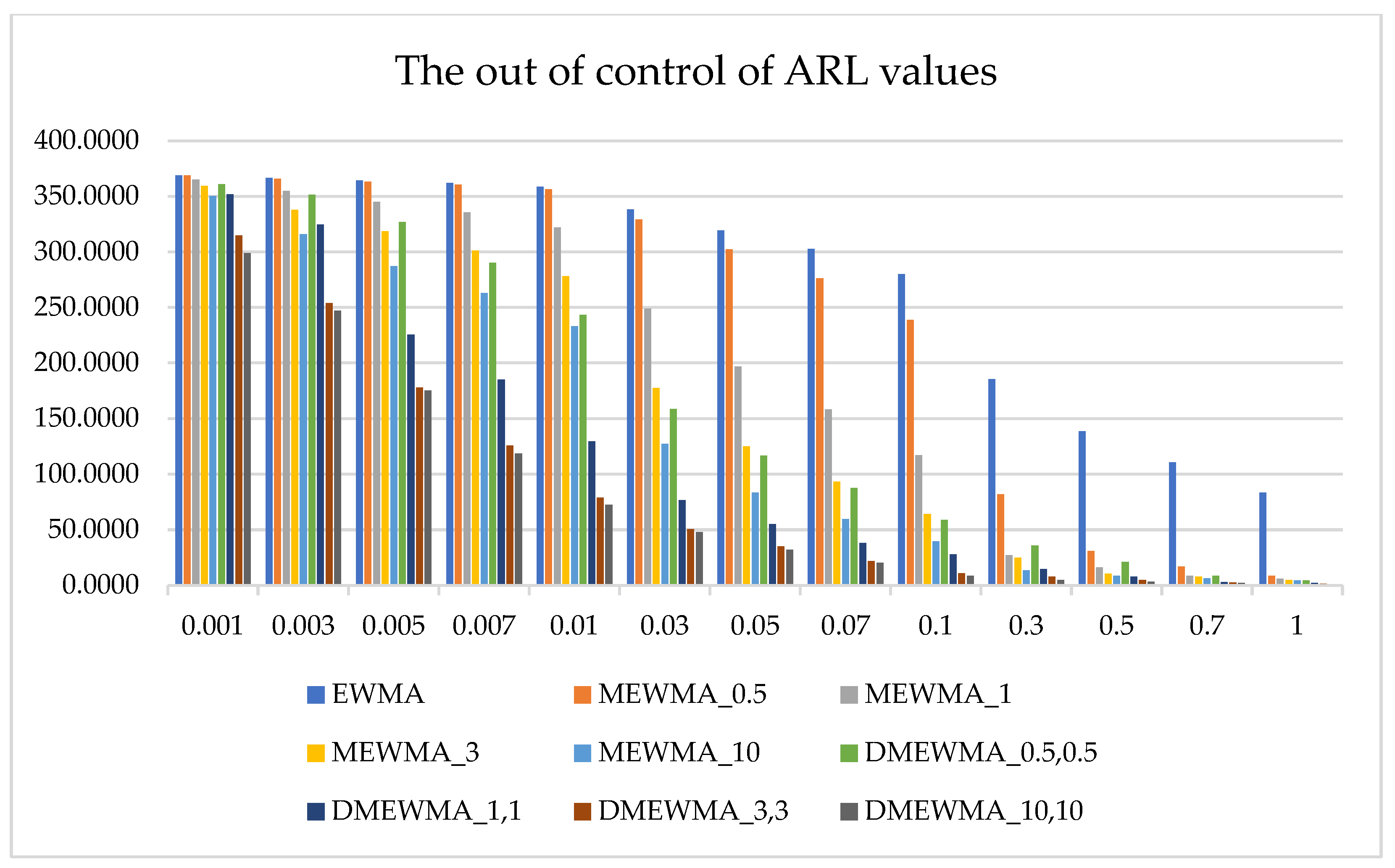
- Compare performance by evaluating the ARL obtained in step 3 with the EWMA and MEWMA control charts.
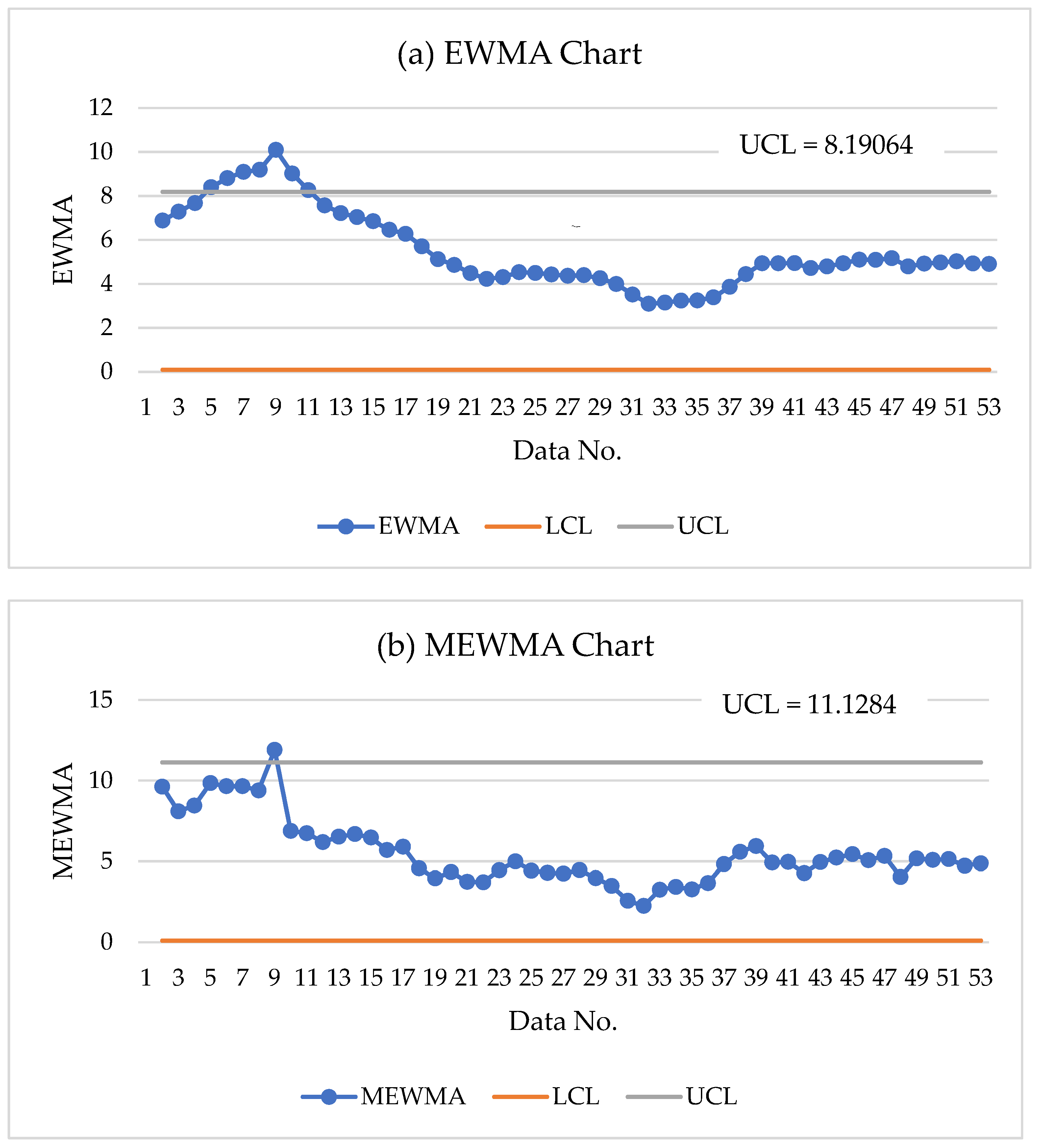
- Detect changes in the process mean by determining the UCL value using the equation in (9) and applying it to data for computation.
- Import AMC Entertainment () stock price data.
- Set initial values and parameters.
- Calculate the statistics for the three control charts using Equations (1)–(3) with the data from step 1.
- Set the upper control limit (UCL) to 0.1.
- Determine the lower control limit (LCL) using Equation (9).
- Plot the graph using the results from steps 3, 4, and 5, and identify any values that exceed the control limits.
4. Discussion and Conclusions
Author Contributions
Funding
Data Availability Statement
Acknowledgments
Conflicts of Interest
References
- Shewhart, W.A. Quality control charts. Bell Syst. Tech. J. 1926, 5, 593–603. [Google Scholar] [CrossRef]
- Pozzi, R.; Cannas, V.G.; Rossi, T. Data Science Supporting Lean Production: Evidence from Manufacturing Companies. Systems 2024, 12, 100. [Google Scholar] [CrossRef]
- Carrey, R.G.; Stake, L.V. Improving Healthcare with Control Charts: Basic and Advanced SPC Methods and Case Studies; ASQ Quality Press: Milwaukee, WI, USA, 2003. [Google Scholar]
- Johan, T.; Jonas, L.; Jakob, A.; Jesper, O.; Cheryl, C.; Karin, P.H.; Mats, B. Application of statistical process control in healthcare improvement: Systematic review. Qual. Saf. Health Care 2007, 16, 387–399. Available online: https://qualitysafety.bmj.com/content/16/5/387 (accessed on 5 November 2024).
- Saravanan, A.; Nagarajan, P. Implementation of quality control charts in bottles manufacturing industry. Int. J. Eng. Sci. Technol. 2013, 5, 335–340. Available online: https://www.semanticscholar.org/paper/IMPLEMENTATION-OF-QUALITY-CONTROL-CHARTS-IN-BOTTLE-Saravanan/a40f7d24bc412debb145f5c3709f6bfe214cdeef#citing-papers (accessed on 20 October 2024).
- Yang, Z. Monitoring Process Variability with Symmetric Control Limits. Research Collection School of Economics, 2020. Available online: https://ink.library.smu.edu.sg/soe_research/2064/ (accessed on 17 December 2024).
- Montgomery, D.C. Introduction to Statistical Quality Control, 8th ed.; Wiley: Hoboken, NJ, USA, 2020. [Google Scholar]
- Page, E.S. Continuous inspection schemes. Biometrika 1954, 41, 100–115. [Google Scholar] [CrossRef]
- Roberts, S.W. Control chart tests based on geometric moving averages. Technometrics 1959, 1, 239–250. [Google Scholar] [CrossRef]
- Shamma, S.E.; Shamma, A.K. Development and evaluation of control charts using double exponentially weighted moving averages. Int. J. Qual. Reliab. Manag. 1992, 9, 18–25. [Google Scholar] [CrossRef]
- Capizzi, G.; Masarotto, G. An adaptive exponentially weighted moving average control chart. Technometrics 2003, 45, 199–207. [Google Scholar] [CrossRef]
- Zhou, Q.; Zou, C.; Wang, Z.; Jiang, W. Likelihoodbased EWMA charts for monitoring poisson count data with time-varying sample sizes. J. Am. Stat. Assoc. 2012, 107, 1049–1062. [Google Scholar] [CrossRef]
- Patel, A.K.; Divecha, J. Modified exponentially weighted moving average (EWMA) control chart for an analytical process data. J. Chem. Eng. Mater. Sci. 2011, 2, 12–20. Available online: https://iopscience.iop.org/article/10.1088/1742-6596/979/1/012097 (accessed on 20 October 2024).
- Naveed, M.; Azam, M.; Khan, N.; Aslam, M. Design a control chart using extended EWMA statistics. Technologies 2018, 6, 108. [Google Scholar] [CrossRef]
- Alevizakos, V.; Chatterjee, K.; Koukouvinos, C. The triple exponentially weighted moving average control chart. Qual. Technol. Quant. Manag. 2021, 18, 326–354. [Google Scholar] [CrossRef]
- Alevizakos, V.; Chatterjee, K.; Koukouvinos, C. Modified EWMA and DEWMA control charts for process monitoring. Commun. Stat. -Theory Methods 2021, 51, 7390–7412. [Google Scholar] [CrossRef]
- Woodall, W.H. Controversies and contradictions in statistical process control. J. Qual. Technol. 2000, 32, 341–350. [Google Scholar] [CrossRef]
- Crowder, S.V. A simple method for studying run length distributions of exponentially weighted moving average charts. Technometrics 1987, 29, 401–407. [Google Scholar] [CrossRef]
- Paichit, P.; Peerajit, W. The average run length for continuous distribution process mean shift detection on a modified EWMA control chart. Asia-Pac. J. Sci. Technol. 2022, 27, 109–118. [Google Scholar] [CrossRef]
- Areepong, Y.; Karoon, K. Detection capability of the dewma chart using explicit run length solutions: A case study on data of gross domestic product. Eng. Lett. 2024, 32, 1300–1312. Available online: https://www.engineeringletters.com/issues_v32/issue_7/index.html (accessed on 20 October 2024).
- Andel, J. On AR (1) processes with exponential white noise. Commun. Stat. Theory Methods 1988, 17, 1481–1495. [Google Scholar] [CrossRef]
- Turkman, M.A.A. Bayesian analysis of an autoregressive process with exponential white noise. Statistics 1990, 21, 601–608. [Google Scholar] [CrossRef]
- Ibazizen, M.; Fellag, H. Bayesian estimation of an AR (1) process with exponential white noise. Statistics 2003, 37, 365–372. [Google Scholar] [CrossRef]
- Girón, F.J.; Caro, E.; Domínguez, J.I. A conjugate family for AR (1) processes with exponential errors. Commun. Stat. Theory Methods 1994, 23, 1771–1784. [Google Scholar] [CrossRef]
- Phanthuna, P.; Areepong, Y.; Sukparungsee, S. Performance Measurement of a DMEWMA Control Chart on an AR(p) Model with Exponential White Noise. Appl. Sci. Eng. Prog. 2024, 17, 7088. [Google Scholar] [CrossRef]
- Neammai, J.; Areepong, Y.; Sukparungsee, S. Performance Comparison of Numerical Integral Equation Methods on DMEWMA Control Chart for Moving Average Process Order q. Research, Invention, and Innovation Congress. In Proceedings of the 2023 Innovative Electricals and Electronics (RI2C), Bangkok, Thailand, 24–25 August 2023. [Google Scholar] [CrossRef]
- Banach Fixed-Point Theorem. Available online: https://en.wikipedia.org/wiki/Banach_fixed-point_theorem (accessed on 4 September 2024).
- Hölder’s Inequality. Available online: https://www.wikiwand.com/en/articles/H%C3%B6lder’s_inequality (accessed on 4 September 2024).
- Bualuang, D.; Peerajit, W. Performance of the CUSUM control chart using approximation to ARL for long-memory fractionally integrated autoregressive process with exogenous variable. Appl. Sci. Eng. Prog. 2022, 16, 5917. [Google Scholar] [CrossRef]
- Fonseca, A.; Ferreira, P.H.; Nascimento, D.C.; Fiaccone, R.; Correa, C.U.; Piña, A.G.; Louzada, F. Water Particles Monitoring in the Atacama Desert: SPC approach Based on proportional data. Axioms 2021, 10, 154. [Google Scholar] [CrossRef]
- Han, D.; Tsung, F. A reference-free cuscore chart for dynamic mean change detection and a unified framework for charting performance comparison. Am. Stat. Assoc. 2006, 101, 368–386. [Google Scholar] [CrossRef]


| MA(1) | MA(2) | MA(3) | ||||||||
| λ1 = 0.05, λ2 = 0.1 | λ1 = 0.1, λ2 = 0.1 | λ1 = 0.2, λ2 = 0.1 | ||||||||
| (u) | (u) | RPC | (u) | (u) | RPC | (u) | (u) | RPC | ||
| 0.00000004651 | 0.0000001415 | 0.0000008574 | ||||||||
| 0.2 | 0 | 370.06599099 | 370.06599097 | 5.40 × 10⁻⁹ | 370.18643108 | 370.18643108 | 0 | 370.00929403 | 370.00929403 | 0 |
| 0.001 | 362.45882162 | 362.45882160 | 5.52 × 10⁻⁹ | 362.96195047 | 362.96195046 | 2.76 × 10⁻⁹ | 363.40862560 | 363.40862560 | 0 | |
| 0.003 | 347.75381070 | 347.75381068 | 5.75 × 10⁻⁹ | 348.97443935 | 348.97443935 | 0 | 350.59608759 | 350.59608759 | 0 | |
| 0.005 | 333.70070787 | 333.70070786 | 2.99 × 10⁻⁹ | 335.57860543 | 335.57860543 | 0 | 338.28350065 | 338.28350065 | 0 | |
| 0.007 | 320.26834537 | 320.26834538 | 3.12 × 10⁻⁹ | 322.74736297 | 322.74736297 | 0 | 326.44961922 | 326.44961922 | 0 | |
| 0.01 | 301.21941228 | 301.21941227 | 3.32 × 10⁻⁹ | 304.50311477 | 304.50311478 | 3.28 × 10⁻⁹ | 309.55227925 | 309.55227925 | 0 | |
| 0.03 | 202.00490775 | 202.00490774 | 4.95 × 10⁻⁹ | 208.40989177 | 208.40989176 | 4.80 × 10⁻⁹ | 218.92831272 | 218.92831272 | 0 | |
| 0.07 | 95.14833819 | 95.14833819 | 0 | 101.97977703 | 101.97977703 | 0 | 113.91462707 | 113.91462707 | 0 | |
| 0.1 | 56.22040234 | 56.22040234 | 0 | 61.85815712 | 61.85815712 | 0 | 72.09160881 | 72.09160881 | 0 | |
| 0.5 | 1.32943633 | 1.32943633 | 0 | 1.47010967 | 1.47010967 | 0 | 1.83226459 | 1.83226459 | 0 | |
| 1 | 1.00904094 | 1.00904094 | 0 | 1.01540939 | 1.01540939 | 0 | 1.03630688 | 1.03630688 | 0 | |
| −0.2 | 0.0000000312 | 0.00000006355 | 0.0000002582 | |||||||
| 0 | 370.34322939 | 370.34322941 | 5.40 × 10⁻⁹ | 370.01220717 | 370.01220717 | 0 | 369.94837505 | 369.94837505 | 0 | |
| 0.001 | 362.58582492 | 362.58582493 | 2.76 × 10⁻⁹ | 362.50209909 | 362.50209909 | 0 | 362.91462183 | 362.91462183 | 0 | |
| 0.003 | 347.59935947 | 347.59935945 | 5.75 × 10⁻⁹ | 347.97894841 | 347.97894840 | 2.87 × 10⁻⁹ | 349.28590317 | 349.28590317 | 0 | |
| 0.005 | 333.28869070 | 333.28869072 | 6.00 × 10⁻⁹ | 334.09229235 | 334.09229235 | 0 | 336.22028669 | 336.22028669 | 0 | |
| 0.007 | 319.62099445 | 319.62099443 | 6.26 × 10⁻⁹ | 320.81202222 | 320.81202223 | 3.12 × 10⁻⁹ | 323.69254849 | 323.69254849 | 0 | |
| 0.01 | 300.25739039 | 300.25739040 | 3.33 × 10⁻⁹ | 301.96646003 | 301.96646002 | 3.31 × 10⁻⁹ | 305.85725787 | 305.85725787 | 0 | |
| 0.03 | 199.82590714 | 199.82590713 | 5.00 × 10⁻⁹ | 203.53715931 | 203.53715932 | 4.91 × 10⁻⁹ | 211.40745707 | 211.40745707 | 0 | |
| 0.07 | 92.78547011 | 92.78547012 | 1.08 × 10⁻⁸ | 96.78542929 | 96.78542929 | 0 | 105.37132431 | 105.37132431 | 0 | |
| 0.1 | 54.28843940 | 54.28843941 | 1.84 × 10⁻⁸ | 57.56243250 | 57.56243249 | 1.74 × 10⁻⁸ | 64.73310077 | 64.73310077 | 0 | |
| 0.5 | 1.28853032 | 1.28853032 | 0 | 1.35989959 | 1.35989959 | 0 | 1.55778367 | 1.55778367 | 0 | |
| 1 | 1.00740765 | 1.00740765 | 0 | 1.01032433 | 1.01032433 | 0 | 1.01992212 | 1.01992212 | 0 | |
| MA(1) | MA(2) | MA(3) | ||||||||
| λ1 = 0.05, λ2 = 0.1 | λ1 = 0.1, λ2 = 0.1 | λ1 = 0.2, λ2 = 0.1 | ||||||||
| (u) | (u) | RPC | (u) | (u) | RPC | (u) | (u) | RPC | ||
| 0.00003971 | 0.00009038 | 0.0003278 | ||||||||
| 0.2 | 0 | 369.60789426 | 369.60789426 | 0 | 370.02499526 | 370.02499526 | 0 | 369.99003541 | 369.99003541 | 0 |
| 0.001 | 364.30292869 | 364.30292869 | 0 | 364.99421498 | 364.99421498 | 0 | 365.39203261 | 365.39203261 | 0 | |
| 0.003 | 353.95053168 | 353.95053168 | 0 | 355.16553942 | 355.16553942 | 0 | 356.39289257 | 356.39289257 | 0 | |
| 0.005 | 343.93126915 | 343.93126915 | 0 | 345.63850270 | 345.63850270 | 0 | 347.64924562 | 347.64924562 | 0 | |
| 0.007 | 334.23326838 | 334.23326838 | 0 | 336.40280558 | 336.40280558 | 0 | 339.15295737 | 339.15295737 | 0 | |
| 0.01 | 320.26379426 | 320.26379426 | 0 | 323.07393700 | 323.07393700 | 0 | 326.85522884 | 326.85522884 | 0 | |
| 0.03 | 242.45417948 | 242.45417948 | 0 | 248.21716517 | 248.21716517 | 0 | 256.90323168 | 256.90323168 | 0 | |
| 0.07 | 143.34883729 | 143.34883729 | 0 | 150.88465547 | 150.88465547 | 0 | 163.00000264 | 163.00000264 | 0 | |
| 0.1 | 99.13343094 | 99.13343094 | 0 | 106.38127708 | 106.38127708 | 0 | 118.41130164 | 118.41130164 | 0 | |
| 0.5 | 3.72430968 | 3.72430968 | 0 | 4.52857694 | 4.52857694 | 0 | 6.25355254 | 6.25355254 | 0 | |
| 1 | 1.21528610 | 1.21528610 | 0 | 1.31727410 | 1.31727410 | 0 | 1.57707711 | 1.57707711 | 0 | |
| −0.2 | 0.00002665 | 0.0000406 | 0.00009861 | |||||||
| 0 | 370.07773148 | 370.07773148 | 0 | 370.04167628 | 370.04167628 | 0 | 369.99862427 | 369.99862427 | 0 | |
| 0.001 | 364.62005491 | 364.62005491 | 0 | 364.71780281 | 364.71780281 | 0 | 364.95619628 | 364.95619628 | 0 | |
| 0.003 | 353.97606978 | 353.97606978 | 0 | 354.32910088 | 354.32910088 | 0 | 355.10543180 | 355.10543180 | 0 | |
| 0.005 | 343.68287666 | 343.68287666 | 0 | 344.27546445 | 344.27546445 | 0 | 345.55783898 | 345.55783898 | 0 | |
| 0.007 | 333.72769914 | 333.72769914 | 0 | 334.54492499 | 334.54492499 | 0 | 336.30303199 | 336.30303199 | 0 | |
| 0.01 | 319.40200743 | 319.40200743 | 0 | 320.52988600 | 320.52988600 | 0 | 322.94803234 | 322.94803234 | 0 | |
| 0.03 | 239.95081009 | 239.95081009 | 0 | 242.49761512 | 242.49761512 | 0 | 247.97850968 | 247.97850968 | 0 | |
| 0.07 | 139.83626953 | 139.83626953 | 0 | 143.20503022 | 143.20503022 | 0 | 150.60020440 | 150.60020440 | 0 | |
| 0.1 | 95.73861116 | 95.73861116 | 0 | 98.95530495 | 98.95530495 | 0 | 106.12358527 | 106.12358527 | 0 | |
| 0.5 | 3.38680948 | 3.38680948 | 0 | 3.70094125 | 3.70094125 | 0 | 4.51244738 | 4.51244738 | 0 | |
| 1 | 1.17645526 | 1.17645526 | 0 | 1.21255789 | 1.21255789 | 0 | 1.31596286 | 1.31596286 | 0 | |
| MA(2) | ||||||||||||
| C1 = C2 = 0.5 | C1 = C2 = 1 | C1 = 1, C2 = 3 | C1 = C2 = 3 | C1 = C2 = 5 | C1 = C2 = 7 | |||||||
| (1) | (2) | (1) | (2) | (1) | (2) | (1) | (2) | (1) | (2) | (1) | (2) | |
| 1.19125 | 0.68373 | 1.677663 | 1.20412 | 2.91761 | 2.47904 | 6.40976 | 6.19054 | 15.6465 | 15.8183 | 29.3889 | 30.0861 | |
| 0 | 369.946 | 369.961 | 370.000 | 370.047 | 370.369 | 370.197 | 369.980 | 370.108 | 369.928 | 370.223 | 370.078 | 370.036 |
| 0.001 | 359.475 | 349.640 | 306.447 | 286.245 | 258.359 | 246.724 | 231.324 | 227.951 | 220.193 | 221.110 | 216.893 | 219.025 |
| 0.003 | 340.129 | 314.903 | 228.127 | 197.083 | 161.192 | 148.224 | 132.508 | 129.208 | 122.002 | 122.775 | 118.986 | 120.914 |
| 0.005 | 322.656 | 286.303 | 181.722 | 150.329 | 117.282 | 106.086 | 93.033 | 90.342 | 84.577 | 85.180 | 82.186 | 83.709 |
| 0.01 | 285.580 | 232.919 | 120.521 | 94.458 | 69.992 | 62.239 | 53.588 | 51.831 | 48.147 | 48.522 | 46.631 | 47.593 |
| 0.03 | 193.342 | 131.564 | 51.512 | 38.212 | 27.250 | 23.915 | 20.393 | 19.670 | 18.212 | 18.354 | 17.611 | 17.988 |
| 0.05 | 144.125 | 90.316 | 32.871 | 24.099 | 17.200 | 15.078 | 12.900 | 12.442 | 11.543 | 11.628 | 11.170 | 11.402 |
| 0.1 | 85.078 | 48.963 | 17.414 | 12.717 | 9.269 | 8.150 | 7.065 | 6.821 | 6.371 | 6.411 | 6.181 | 6.297 |
| 0.3 | 27.870 | 15.255 | 6.378 | 4.769 | 3.784 | 3.386 | 3.063 | 2.972 | 2.834 | 2.843 | 2.771 | 2.807 |
| 0.5 | 15.248 | 8.451 | 4.138 | 3.177 | 2.670 | 2.423 | 2.250 | 2.191 | 2.114 | 2.118 | 2.077 | 2.097 |
| 1 | 6.690 | 3.926 | 2.495 | 2.020 | 1.833 | 1.703 | 1.633 | 1.600 | 1.567 | 1.568 | 1.549 | 1.558 |
| MA(3) | ||||||||||||
| C1 = C2 = 0.5 | C1 = C2 = 1 | C1 = 1, C2 = 3 | C1 = C2 = 3 | C1 = C2 = 5 | C1 = C2 = 7 | |||||||
| (1) | (2) | (1) | (2) | (1) | (2) | (1) | (2) | (1) | (2) | (1) | (2) | |
| 1.23761 | 0.72789 | 1.83392 | 1.37127 | 3.35807 | 2.94963 | 7.65116 | 7.54494 | 19.00647 | 19.46550 | 35.90100 | 37.13110 | |
| 0 | 370.135 | 370.419 | 369.872 | 369.884 | 369.901 | 370.228 | 370.063 | 369.964 | 369.936 | 370.183 | 370.587 | 369.902 |
| 0.001 | 359.131 | 349.236 | 305.571 | 287.899 | 260.532 | 252.211 | 236.817 | 235.495 | 227.172 | 229.531 | 224.545 | 227.654 |
| 0.003 | 328.890 | 313.268 | 226.789 | 199.555 | 163.936 | 154.247 | 137.966 | 136.655 | 128.532 | 130.733 | 125.900 | 128.999 |
| 0.005 | 320.705 | 283.882 | 180.347 | 152.763 | 119.749 | 111.254 | 97.529 | 96.446 | 89.824 | 91.595 | 87.682 | 90.202 |
| 0.01 | 282.422 | 229.569 | 119.367 | 96.421 | 71.780 | 65.804 | 56.564 | 55.844 | 51.533 | 52.672 | 50.143 | 51.776 |
| 0.03 | 188.921 | 128.339 | 50.968 | 39.222 | 28.081 | 25.468 | 21.650 | 21.343 | 19.606 | 20.059 | 19.044 | 19.701 |
| 0.05 | 140.016 | 87.826 | 32.554 | 24.793 | 17.757 | 16.083 | 13.711 | 13.512 | 12.435 | 12.714 | 12.085 | 12.493 |
| 0.1 | 82.204 | 47.579 | 17.303 | 13.130 | 9.595 | 8.702 | 7.513 | 7.401 | 6.858 | 6.998 | 6.678 | 6.886 |
| 0.3 | 26.990 | 14.974 | 6.409 | 4.958 | 3.937 | 3.609 | 3.250 | 3.202 | 3.031 | 3.074 | 2.971 | 3.038 |
| 0.5 | 14.863 | 8.375 | 4.188 | 3.312 | 2.781 | 2.573 | 2.378 | 2.344 | 2.248 | 2.272 | 2.212 | 2.251 |
| 1 | 6.609 | 3.948 | 2.546 | 2.103 | 1.905 | 1.792 | 1.711 | 1.690 | 1.648 | 1.658 | 1.630 | 1.649 |
| MA(2): for θ1, θ2 | MA(3): for θ1, θ2, θ3 | |||||||
|---|---|---|---|---|---|---|---|---|
| C1 = 0.5, C2 = 1 | C1 = 3, C2 = 5 | C1 = 0.5, C2 = 1 | C1 = 3, C2 = 5 | |||||
| (1) | (2) | (1) | (2) | (1) | (2) | (1) | (2) | |
| b= 0.285341 | 0.31621 | 8.70184 | 9.64651 | 0.35053 | 0.53124 | 10.69735 | 16.246 | |
| 0 | 370.00410 | 369.66375 | 369.85936 | 369.96074 | 370.20447 | 369.86214 | 370.07235 | 370.28991 |
| 0.001 | 313.39718 | 315.03276 | 218.07332 | 221.95416 | 317.35045 | 325.43850 | 226.04914 | 245.58710 |
| 0.003 | 239.81202 | 243.00997 | 120.08458 | 123.61481 | 246.71736 | 262.28665 | 127.42626 | 147.04708 |
| 0.005 | 194.07388 | 197.65861 | 83.05387 | 85.86232 | 201.67451 | 219.55192 | 88.92141 | 105.14325 |
| 0.01 | 131.14285 | 134.51258 | 47.17362 | 48.96813 | 138.21413 | 155.76894 | 50.93950 | 61.69997 |
| 0.03 | 56.40056 | 58.36532 | 17.81168 | 18.54302 | 60.51030 | 71.36048 | 19.35152 | 23.85669 |
| 0.05 | 35.52137 | 36.86424 | 11.28574 | 11.75174 | 38.33003 | 45.86147 | 12.26730 | 15.14393 |
| 0.1 | 18.06242 | 18.80236 | 6.22934 | 6.48188 | 19.60991 | 23.79975 | 6.76114 | 8.31130 |
| 0.3 | 5.80729 | 6.06211 | 2.77480 | 2.87531 | 6.34012 | 7.77954 | 2.98612 | 3.58787 |
| 0.5 | 3.50075 | 3.64982 | 2.07356 | 2.14097 | 3.81255 | 4.65230 | 2.21520 | 2.61326 |
| 1 | 1.98438 | 2.05395 | 1.54293 | 1.58269 | 2.13006 | 2.52223 | 1.62647 | 1.85809 |
| Chart | EWMA | MEWMA (c) | DMEWMA (c1, c2) | ||||||||
|---|---|---|---|---|---|---|---|---|---|---|---|
| 0.5 | 1 | 3 | 10 | 0.5, 0.5 | 1, 1 | 1, 3 | 3, 3 | 10, 10 | |||
| b = 0.10000379 | 0.80751 | 0.65675 | 0.959455 | 2.34905 | 1.64661 | 6.32246 | 9.7581 | 29.189 | 86.4675 | ||
| 0.001 | ARLout | 364.6455 | 335.9040 | 276.2000 | 217.4547 | 215.3046 | 308.9601 | 231.5981 | 224.7168 | 216.9983 | 214.3852 |
| SDRLout | 364.1452 | 335.4037 | 275.6995 | 216.9541 | 214.8040 | 308.4596 | 231.0975 | 224.2162 | 216.4978 | 213.8846 | |
| MRLout | 252.4063 | 232.4842 | 191.1004 | 150.3812 | 148.8909 | 213.8080 | 160.1847 | 155.4150 | 150.0649 | 148.2537 | |
| 0.003 | ARLout | 352.9561 | 283.7107 | 183.2607 | 119.5263 | 117.4893 | 232.3062 | 132.7764 | 126.1784 | 119.0332 | 116.7953 |
| SDRLout | 352.4558 | 283.2103 | 182.7600 | 119.0252 | 116.9883 | 231.8057 | 132.2754 | 125.6774 | 118.5322 | 116.2942 | |
| MRLout | 244.3038 | 196.3065 | 126.6798 | 82.5022 | 81.0903 | 160.6756 | 91.6865 | 87.1131 | 82.1605 | 80.6093 | |
| 0.005 | ARLout | 341.6854 | 245.4477 | 137.1517 | 82.6188 | 80.9325 | 186.1505 | 93.2524 | 87.9109 | 82.2149 | 80.4684 |
| SDRLout | 341.1850 | 244.9472 | 136.6508 | 82.1173 | 80.4309 | 185.6499 | 92.7510 | 87.4095 | 81.7134 | 79.9668 | |
| MRLout | 236.4915 | 169.7846 | 94.7193 | 56.9197 | 55.7508 | 128.6828 | 64.2904 | 60.5880 | 56.6398 | 55.4291 | |
| 0.01 | ARLout | 315.2342 | 183.2973 | 84.2463 | 46.9103 | 45.7227 | 124.4193 | 53.7310 | 50.2750 | 46.6462 | 45.5538 |
| SDRLout | 314.7338 | 182.7966 | 83.7448 | 46.4076 | 45.2200 | 123.9183 | 53.2286 | 49.7725 | 46.1435 | 45.0511 | |
| MRLout | 218.1569 | 126.7051 | 58.0478 | 32.1679 | 31.3447 | 85.8938 | 36.8958 | 34.5003 | 31.9849 | 31.2277 | |
| 0.03 | ARLout | 230.1697 | 90.1858 | 33.2579 | 17.7268 | 17.2096 | 53.6114 | 20.4513 | 19.0594 | 17.6160 | 17.1874 |
| SDRLout | 229.6691 | 89.6844 | 32.7541 | 17.2195 | 16.7021 | 53.1091 | 19.9451 | 18.5527 | 17.1087 | 16.6799 | |
| MRLout | 159.1946 | 62.1648 | 22.7043 | 11.9373 | 11.5788 | 36.8129 | 13.8263 | 12.8613 | 11.8605 | 11.5633 | |
| 0.05 | ARLout | 170.0919 | 59.2364 | 20.8099 | 11.2447 | 10.9225 | 34.2623 | 12.9363 | 12.0696 | 11.1728 | 10.9072 |
| SDRLout | 169.5912 | 58.7343 | 20.3037 | 10.7331 | 10.4105 | 33.7586 | 12.4263 | 11.5588 | 10.6611 | 10.3952 | |
| MRLout | 117.5518 | 40.7120 | 14.0749 | 7.4423 | 7.2188 | 23.4005 | 8.6156 | 8.0144 | 7.3924 | 7.2082 | |
| 0.1 | ARLout | 83.8687 | 31.2683 | 10.8799 | 6.2226 | 6.0564 | 18.1471 | 7.0834 | 6.6404 | 6.1822 | 6.0467 |
| SDRLout | 83.3672 | 30.7643 | 10.3679 | 5.7007 | 5.5339 | 17.6400 | 6.5644 | 6.1200 | 5.6602 | 5.5241 | |
| MRLout | 57.7861 | 21.3251 | 7.1893 | 3.9565 | 3.8410 | 12.2288 | 4.5545 | 4.2467 | 3.9284 | 3.8342 | |
| 0.3 | ARLout | 39.1365 | 10.2073 | 4.0399 | 2.7886 | 2.7315 | 6.6076 | 3.0695 | 2.9231 | 2.7711 | 2.7261 |
| SDRLout | 38.6333 | 9.6945 | 3.5044 | 2.2333 | 2.1747 | 6.0871 | 2.5204 | 2.3709 | 2.2154 | 2.1692 | |
| MRLout | 26.7793 | 6.7227 | 2.4373 | 1.5608 | 1.5205 | 4.2240 | 1.7583 | 1.6554 | 1.5485 | 1.5167 | |
| 0.5 | ARLout | 22.4532 | 6.0078 | 2.7021 | 2.0892 | 2.0544 | 4.2655 | 2.2531 | 2.1668 | 2.0770 | 2.0503 |
| SDRLout | 21.9475 | 5.4850 | 2.1446 | 1.5085 | 1.4718 | 3.7322 | 1.6803 | 1.5901 | 1.4956 | 1.4674 | |
| MRLout | 15.2142 | 3.8072 | 1.4998 | 1.0642 | 1.0392 | 2.5947 | 1.1815 | 1.1198 | 1.0554 | 1.0362 | |
| 1 | ARLout | 6.0837 | 3.1175 | 1.7578 | 1.5569 | 1.5392 | 2.5503 | 1.6348 | 1.5931 | 1.5494 | 1.5363 |
| SDRLout | 5.5613 | 2.5693 | 1.1542 | 0.9311 | 0.9110 | 1.9884 | 1.0187 | 0.9720 | 0.9226 | 0.9077 | |
| MRLout | 3.8600 | 1.7920 | 0.8238 | 0.6742 | 0.6608 | 1.3925 | 0.7327 | 0.7015 | 0.6685 | 0.6586 | |
| Chart | EWMA | MEWMA (c) | DMEWMA (c1, c2) | ||||||||
|---|---|---|---|---|---|---|---|---|---|---|---|
| 0.5 | 1 | 3 | 10 | 0.5, 0.5 | 1, 1 | 1, 3 | 3, 3 | 10, 10 | |||
| b = 0.15143 | 0.97119 | 0.782202 | 1.15148 | 1.62678 | 1.79576 | 3.25073 | 18.83 | 51.2787 | 80.035 | ||
| 0.001 | ARLout | 367.6157 | 342.3886 | 281.8298 | 221.5179 | 207.3860 | 307.9553 | 262.0984 | 227.5443 | 220.7706 | 201.5782 |
| SDRLout | 367.1154 | 341.8882 | 281.3294 | 221.0173 | 206.8853 | 307.4549 | 261.5980 | 227.0438 | 220.2700 | 201.0775 | |
| MRLout | 254.4651 | 236.9790 | 195.0028 | 153.1977 | 143.4021 | 213.1116 | 181.3260 | 157.3749 | 152.6797 | 139.3765 | |
| 0.003 | ARLout | 362.8827 | 297.5887 | 190.8726 | 123.2368 | 110.6148 | 230.7788 | 165.7873 | 128.6869 | 122.3759 | 103.2890 |
| SDRLout | 362.3823 | 297.0882 | 190.3720 | 122.7358 | 110.1137 | 230.2782 | 165.2865 | 128.1859 | 121.8749 | 102.7878 | |
| MRLout | 251.1844 | 205.9260 | 131.9559 | 85.0742 | 76.3252 | 159.6168 | 114.5681 | 88.8519 | 84.4775 | 71.2473 | |
| 0.005 | ARLout | 358.2276 | 263.0402 | 144.3368 | 85.5768 | 75.5907 | 184.5699 | 121.3882 | 89.9171 | 84.4821 | 75.4170 |
| SDRLout | 357.7272 | 262.5397 | 143.8360 | 85.0753 | 75.0890 | 184.0692 | 120.8871 | 89.4157 | 83.9806 | 74.9153 | |
| MRLout | 247.9577 | 181.9788 | 99.6997 | 58.9700 | 52.0481 | 127.5872 | 83.7928 | 61.9786 | 58.2113 | 51.9277 | |
| 0.01 | ARLout | 346.9212 | 203.5693 | 89.7391 | 48.8102 | 42.4215 | 123.0718 | 72.9440 | 51.5778 | 48.3852 | 42.1341 |
| SDRLout | 346.4209 | 203.0687 | 89.2377 | 48.3076 | 41.9185 | 122.5708 | 72.4423 | 51.0753 | 47.8825 | 41.6311 | |
| MRLout | 240.1207 | 140.7566 | 61.8552 | 33.4849 | 29.0564 | 84.9598 | 50.2136 | 35.4033 | 33.1903 | 28.8572 | |
| 0.03 | ARLout | 306.0328 | 105.7627 | 35.8594 | 18.5175 | 15.8245 | 52.9551 | 28.5889 | 19.6195 | 18.3440 | 15.5245 |
| SDRLout | 305.5324 | 105.2615 | 35.3559 | 18.0106 | 15.3163 | 52.4527 | 28.0844 | 19.1130 | 17.8370 | 15.0162 | |
| MRLout | 211.7790 | 72.9620 | 24.5076 | 12.4856 | 10.6183 | 36.3580 | 19.4677 | 13.2496 | 12.3653 | 10.4103 | |
| 0.05 | ARLout | 271.1569 | 70.6712 | 22.5106 | 11.7585 | 9.9808 | 33.8713 | 18.0788 | 12.4429 | 11.0979 | 9.7613 |
| SDRLout | 270.6564 | 70.1694 | 22.0049 | 11.2474 | 9.4676 | 33.3675 | 17.5717 | 11.9324 | 10.5861 | 9.2478 | |
| MRLout | 187.6048 | 48.6382 | 15.2539 | 7.7987 | 6.5655 | 23.1295 | 12.1814 | 8.2733 | 7.3405 | 6.4132 | |
| 0.1 | ARLout | 203.9691 | 37.7609 | 11.8021 | 6.5131 | 5.4747 | 17.9980 | 9.7609 | 6.8621 | 6.4827 | 5.3127 |
| SDRLout | 203.4685 | 37.2576 | 11.2910 | 5.9922 | 4.9495 | 17.4909 | 9.2474 | 6.3424 | 5.9618 | 4.7866 | |
| MRLout | 141.0337 | 25.8257 | 7.8289 | 4.1583 | 3.4365 | 12.1254 | 6.4129 | 4.4007 | 4.1372 | 3.3238 | |
| 0.3 | ARLout | 79.9738 | 12.2468 | 4.3800 | 2.9177 | 2.4258 | 6.6284 | 3.9912 | 3.0326 | 2.8990 | 2.3155 |
| SDRLout | 79.4722 | 11.7361 | 3.8476 | 2.3654 | 1.8598 | 6.1079 | 3.4552 | 2.4827 | 2.3463 | 1.7453 | |
| MRLout | 55.0863 | 8.1373 | 2.6744 | 1.6517 | 1.3043 | 4.2384 | 2.4033 | 1.7324 | 1.6385 | 1.2259 | |
| 0.5 | ARLout | 39.5154 | 7.1083 | 2.9152 | 2.1814 | 1.8224 | 4.3105 | 2.8127 | 2.2489 | 2.1731 | 1.7908 |
| SDRLout | 39.0122 | 6.5893 | 2.3629 | 1.6053 | 1.2242 | 3.7775 | 2.2580 | 1.6759 | 1.5967 | 1.1900 | |
| MRLout | 27.0419 | 4.5717 | 1.6499 | 1.1303 | 0.8711 | 2.6260 | 1.5777 | 1.1784 | 1.1243 | 0.8480 | |
| 1 | ARLout | 12.1688 | 3.5780 | 1.8698 | 1.6159 | 1.3837 | 2.5993 | 1.9199 | 1.6483 | 1.6085 | 1.3793 |
| SDRLout | 11.6581 | 3.0371 | 1.2753 | 0.9977 | 0.7286 | 2.0388 | 1.3290 | 1.0337 | 0.9893 | 0.7233 | |
| MRLout | 8.0833 | 2.1146 | 0.9057 | 0.7186 | 0.5404 | 1.4271 | 0.9421 | 0.7428 | 0.7131 | 0.5369 | |
| Control Charts | C1 | C2 | MA(2) | MA(3) | ||
|---|---|---|---|---|---|---|
| RMI | RSDI | RMI | RSDI | |||
| EWMA | - | - | 7.801 | 9.005 | 15.963 | 19.501 |
| MEWMA | 0.5 | - | 2.562 | 2.876 | 3.591 | 4.181 |
| 1 | - | 0.600 | 0.657 | 0.900 | 1.036 | |
| 3 | - | 0.024 | 0.027 | 0.186 | 0.234 | |
| 10 | - | 0.003 | 0.003 | 0.025 | 0.029 | |
| DMEWMA | 0.5 | 0.5 | 1.390 | 1.567 | 1.655 | 1.942 |
| 1 | 1 | 0.139 | 0.157 | 0.646 | 0.768 | |
| 1 | 3 | 0.080 | 0.091 | 0.238 | 0.294 | |
| 3 | 3 | 0.019 | 0.021 | 0.172 | 0.218 | |
| 10 | 10 | 0.000 | 0.000 | 0.000 | 0.000 | |
| Model | Model Parameters | Model Statistics | ||||||
|---|---|---|---|---|---|---|---|---|
| Constant | Lag1 | Lag2 | Lag3 | R2 | RMSE | MAPE | MAE | |
| MA(1) | 5.535 | −0.732 | - | - | 0.554 | 1.270 | 17.821 | 0.956 |
| MA(2) | 5.550 | −0.993 | −0.633 | - | 0.728 | 1.003 | 13.247 | 0.728 |
| MA(3) | 5.606 | −1.119 | −0.974 | −0.397 | 0.774 | 0.922 | 11.185 | 0.625 |
| Model | Exponential Parameter | Sig |
|---|---|---|
| MA(3) | 0.7647 | 0.157 |
| Charts | EWMA | MEWMA (c) | DMEWMA (c1, c2) | |||||||
|---|---|---|---|---|---|---|---|---|---|---|
| 0.5 | 1 | 3 | 10 | 0.5, 0.5 | 1, 1 | 3, 3 | 10, 10 | |||
| b = 0.12398 | 2.02348 | 2.011 | 2.00206 | 1.9621 | 1.47694 | 3.99586 | 28.4216 | 90.1302 | ||
| 0 | ARLin | 369.91654 | 369.99253 | 370.15477 | 370.72015 | 369.9703 | 370.2553 | 370.0693 | 369.9847 | 370.0226 |
| SDRLin | 369.4162 | 369.4922 | 369.6544 | 370.2198 | 369.4700 | 369.7550 | 369.5689 | 369.4844 | 369.5222 | |
| MRLin | 256.0599 | 256.1125 | 256.2250 | 256.6169 | 256.0971 | 256.2947 | 256.1657 | 256.1071 | 256.1334 | |
| 0.001 | ARLout | 368.77143 | 368.64605 | 364.89692 | 359.15517 | 350.1337 | 360.9612 | 351.9256 | 314.7130 | 299.0203 |
| SDRLout | 368.2711 | 368.1457 | 364.3966 | 358.6548 | 349.6333 | 360.4609 | 351.4252 | 314.2126 | 298.5198 | |
| MRLout | 255.2661 | 255.1792 | 252.5805 | 248.6007 | 242.3474 | 249.8525 | 243.5895 | 217.7957 | 206.9183 | |
| 0.003 | ARLout | 366.49964 | 365.94901 | 354.69450 | 337.81776 | 315.8523 | 351.3734 | 324.6360 | 253.6623 | 247.0180 |
| SDRLout | 365.9993 | 365.4487 | 354.1941 | 337.3174 | 315.3519 | 350.8730 | 324.1356 | 253.1618 | 246.5175 | |
| MRLout | 253.6915 | 253.3098 | 245.5088 | 233.8107 | 218.5854 | 243.2067 | 224.6737 | 175.4785 | 170.8731 | |
| 0.005 | ARLout | 364.25214 | 363.24699 | 344.89113 | 318.58003 | 287.2715 | 326.7858 | 225.3434 | 178.0265 | 175.3567 |
| SDRLout | 363.7518 | 362.7466 | 344.3908 | 318.0796 | 286.7711 | 326.2855 | 224.8428 | 177.5258 | 174.8560 | |
| MRLout | 252.1336 | 251.4369 | 238.7136 | 220.4761 | 198.7747 | 226.1639 | 155.8493 | 123.0517 | 121.2011 | |
| 0.007 | ARLout | 362.02860 | 360.54052 | 335.46576 | 301.15003 | 263.0832 | 290.1986 | 185.0478 | 125.7999 | 118.4053 |
| SDRLout | 361.5283 | 360.0402 | 334.9654 | 300.6496 | 262.5827 | 289.6982 | 184.5471 | 125.2989 | 117.9043 | |
| MRLout | 250.5924 | 249.5609 | 232.1804 | 208.3945 | 182.0086 | 200.8036 | 127.9185 | 86.8508 | 81.7253 | |
| 0.01 | ARLout | 358.73747 | 356.47370 | 321.99390 | 277.88039 | 233.0584 | 243.3182 | 129.5987 | 78.9768 | 72.1781 |
| SDRLout | 358.2371 | 355.9733 | 321.4935 | 277.3799 | 232.5578 | 242.8177 | 129.0978 | 78.4752 | 71.6764 | |
| MRLout | 248.3111 | 246.7420 | 222.8424 | 192.2652 | 161.1969 | 168.3085 | 89.4840 | 54.3952 | 49.6827 | |
| 0.03 | ARLout | 338.07575 | 329.27247 | 248.85699 | 177.58718 | 127.1687 | 158.4546 | 76.4265 | 50.5188 | 47.7907 |
| SDRLout | 337.5754 | 328.7721 | 248.3565 | 177.0865 | 126.6677 | 157.9538 | 75.9249 | 50.0163 | 47.2880 | |
| MRLout | 233.9895 | 227.8875 | 172.1477 | 122.7472 | 87.7996 | 109.4854 | 52.6275 | 34.6692 | 32.7782 | |
| Charts | EWMA | MEWMA (c) | DMEWMA (c1, c2) | |||||||
| 0.5 | 1 | 3 | 10 | 0.5, 0.5 | 1, 1 | 3, 3 | 10, 10 | |||
| B = 0.12398 | 2.02348 | 2.011 | 2.00206 | 1.9621 | 1.819064 | 4.37942 | 32.2921 | 88.978 | ||
| 0.05 | ARLout | 319.43208 | 302.28887 | 196.67406 | 125.01030 | 83.2433 | 116.5744 | 54.9317 | 34.9291 | 31.9074 |
| SDRLout | 318.9317 | 301.7885 | 196.1734 | 124.5093 | 82.7418 | 116.0733 | 54.4294 | 34.4255 | 31.4034 | |
| MRLout | 221.0667 | 209.1839 | 135.9772 | 86.3035 | 57.3526 | 80.4562 | 37.7281 | 23.8628 | 21.7681 | |
| 0.07 | ARLout | 302.55307 | 275.99674 | 158.18133 | 93.10998 | 59.5376 | 87.6432 | 38.1022 | 21.6339 | 20.2366 |
| SDRLout | 302.0527 | 275.4963 | 157.6805 | 92.6086 | 59.0355 | 87.1418 | 37.5988 | 21.1280 | 19.7303 | |
| MRLout | 209.3670 | 190.9596 | 109.2960 | 64.1917 | 40.9208 | 60.4024 | 26.0623 | 14.6462 | 13.6774 | |
| 0.1 | ARLout | 280.08034 | 238.69328 | 117.10408 | 63.97491 | 39.55221 | 58.5818 | 27.7200 | 10.9154 | 8.5243 |
| SDRLout | 279.5799 | 238.1928 | 116.6030 | 63.4729 | 39.0490 | 58.0797 | 27.2154 | 10.4034 | 8.0087 | |
| MRLout | 193.7901 | 165.1028 | 80.8233 | 43.9965 | 27.0675 | 40.2582 | 18.8654 | 7.2139 | 5.5548 | |
| 0.3 | ARLout | 185.51563 | 81.75042 | 26.83266 | 24.90194 | 13.4499 | 35.5645 | 14.6515 | 7.7634 | 4.5832 |
| SDRLout | 185.0150 | 81.2489 | 26.3279 | 24.3968 | 12.9402 | 35.0610 | 14.1426 | 7.2462 | 4.0524 | |
| MRLout | 128.2428 | 56.3178 | 18.2502 | 16.9118 | 8.9717 | 24.3032 | 9.8050 | 5.0266 | 2.8160 | |
| 0.5 | ARLout | 138.36034 | 30.82622 | 15.94643 | 10.18304 | 8.3159 | 21.0450 | 7.7915 | 4.6546 | 3.0417 |
| SDRLout | 137.8594 | 30.3221 | 15.4383 | 9.6701 | 7.7999 | 20.5389 | 7.2744 | 4.1244 | 2.4920 | |
| MRLout | 95.5571 | 21.0186 | 10.7029 | 6.7058 | 5.4102 | 14.2379 | 5.0462 | 2.8658 | 1.7388 | |
| 0.7 | ARLout | 110.41873 | 16.65663 | 8.56165 | 7.86115 | 6.1066 | 8.6037 | 2.6817 | 2.3524 | 2.0872 |
| SDRLout | 109.9176 | 16.1489 | 8.0461 | 7.3441 | 5.5843 | 8.0882 | 2.1237 | 1.7836 | 1.5064 | |
| MRLout | 76.1893 | 11.1953 | 5.5807 | 5.0945 | 3.8759 | 5.6099 | 1.4854 | 1.2521 | 1.0628 | |
| 1 | ARLout | 83.44615 | 8.58630 | 5.96060 | 4.79052 | 4.4676 | 4.1556 | 1.9847 | 1.4316 | 1.0352 |
| SDRLout | 82.9446 | 8.0708 | 5.4377 | 4.2613 | 3.9360 | 3.6213 | 1.3980 | 0.7861 | 0.1908 | |
| MRLout | 57.4932 | 5.5978 | 3.7744 | 2.9604 | 2.7355 | 2.5180 | 0.9890 | 0.5781 | 0.2049 | |
| RMI | 28.419 | 10.202 | 5.280 | 3.469 | 2.230 | 3.830 | 1.155 | 0.249 | 0.000 | |
| RSDI | 67.603 | 14.531 | 7.954 | 5.525 | 4.040 | 5.729 | 1.793 | 0.55232 | 0 | |
Disclaimer/Publisher’s Note: The statements, opinions and data contained in all publications are solely those of the individual author(s) and contributor(s) and not of MDPI and/or the editor(s). MDPI and/or the editor(s) disclaim responsibility for any injury to people or property resulting from any ideas, methods, instructions or products referred to in the content. |
© 2025 by the authors. Licensee MDPI, Basel, Switzerland. This article is an open access article distributed under the terms and conditions of the Creative Commons Attribution (CC BY) license (https://creativecommons.org/licenses/by/4.0/).
Share and Cite
Neammai, J.; Sukparungsee, S.; Areepong, Y. Explicit Analytical Form for the Average Run Length of Double-Modified Exponentially Weighted Moving Average Control Charts Through the MA(q) Process and Applications. Symmetry 2025, 17, 238. https://doi.org/10.3390/sym17020238
Neammai J, Sukparungsee S, Areepong Y. Explicit Analytical Form for the Average Run Length of Double-Modified Exponentially Weighted Moving Average Control Charts Through the MA(q) Process and Applications. Symmetry. 2025; 17(2):238. https://doi.org/10.3390/sym17020238
Chicago/Turabian StyleNeammai, Julalak, Saowanit Sukparungsee, and Yupaporn Areepong. 2025. "Explicit Analytical Form for the Average Run Length of Double-Modified Exponentially Weighted Moving Average Control Charts Through the MA(q) Process and Applications" Symmetry 17, no. 2: 238. https://doi.org/10.3390/sym17020238
APA StyleNeammai, J., Sukparungsee, S., & Areepong, Y. (2025). Explicit Analytical Form for the Average Run Length of Double-Modified Exponentially Weighted Moving Average Control Charts Through the MA(q) Process and Applications. Symmetry, 17(2), 238. https://doi.org/10.3390/sym17020238