Article

Equal Division Contribution Values of Trapezoidal Fuzzy Numbers and Their Application to Profit Allocation in Cold Chain Logistics for Agricultural Products

by
Jungan Zhan
1,
Rong Fan
2,
Minghao Liu
2,
Jiacai Liu
1,2 and
Wenjian Zhao
1,*
1
Jinshan College, Fujian Agriculture and Forestry University, Fuzhou 350002, China
2
College of Transportation and Civil Engineering, Fujian Agriculture and Forestry University, Fuzhou 350108, China
*
Author to whom correspondence should be addressed.
Symmetry 2025, 17(2), 210; https://doi.org/10.3390/sym17020210
Submission received: 24 December 2024 / Revised: 23 January 2025 / Accepted: 24 January 2025 / Published: 29 January 2025
(This article belongs to the Section Computer)

Abstract

:
With the acceleration of fresh food e-commerce development, cold chain logistics for agricultural products has increasingly become a research hotspot. However, limited by the number of orders accepted by enterprises, many cold chain transportation vehicles for agricultural products struggle to reach a full load. This undoubtedly increases transportation costs for agricultural product cold chain logistics enterprises. In order to reduce the cost of transportation and increase the profit of enterprises, this paper will adopt the strategy of building enterprise coalition based on cooperative game theory. By increasing the loading rate of transportation vehicles, it will increase the profit of enterprises. First, utilizing the minimization of overall dissatisfaction among players in profit allocation after coalition participation as the objective function, a model of the equal division contribution values of the trapezoidal fuzzy number will be constructed, which will be used as the profit allocation model for the players. Then, the solution of the model will be provided, and the properties including symmetry are analyzed. Second, by improving the loading rate of cold chain transport vehicles as the key and combining various parameters in the transportation stage of agricultural product cold chain logistics, the coalition profit will be calculated. Finally, using the solution of the equal division contribution value of the trapezoidal fuzzy number in the cooperative game as the allocation strategy, the obtained profit will be distributed to each enterprise participating in the coalition. The results show that when dealing with cooperative profit allocation problems in similar scenarios, the solutions of the equal division contribution value of the trapezoidal fuzzy number are highly reliable and adaptable. The method presented in this paper can not only increase the profit of enterprises but also minimize the overall dissatisfaction of all enterprises with the allocation result.

1. Introduction

The high transportation costs of cold chain logistics for agricultural products have always been a complicated issue. Particularly for small and medium-sized enterprises, due to their limitations in brand influence, it is rather difficult to receive enough transportation orders to fill the cold chain transport vehicles. The inability to fully load cold chain transport vehicles results in low utilization rates of the vehicles, which increase the transportation costs of enterprises and reduce their profit. Specifically, there is a road distance of about 960 km from Changsha to Shenzhen. Over such a long stretch of road, taking into account explicit and implicit factors such as fuel consumption and vehicle depreciation, the difference in transportation costs between a half load and a full load for just the outbound trip may be about 15%. Therefore, this paper proposes a method to reduce transportation costs for agricultural product cold chain logistics enterprises through a cooperative game. The purpose is to increase the overall profit of the coalition through cooperation and then allocate a fair and reasonable profit for each enterprise participating in the coalition.
In recent years, scholars [1,2] have found that in practical cooperative game problems, due to numerous uncertainties in aspects such as the market, players, and external environment, it is difficult to express the profit values of cooperative coalitions with precise numbers. Therefore, in order to meet practical needs, it is necessary to conduct in-depth research on new solutions to the cooperative game in fuzzy environments.
Based on the above considerations, this paper puts forward a model of the equal division contribution value of the trapezoidal fuzzy number in a fuzzy environment, presents the solution of the model, and analyzes the properties of the solution. Then, on the basis of this model, taking a cooperative coalition of three small and medium-sized agricultural product cold chain logistics enterprises as a case, the one-way transportation costs and profits for the coalition are calculated. Finally, the profits of the coalition are allocated to each player.
This paper makes at least two innovations to the field of cold chain logistics and cooperative game research, as follows.
In the field of cold chain logistics for agricultural products, most of the existing research takes the identification of problems within enterprises as the starting point and aims to increase an enterprise’s profit by solving their own problems and changing their own conditions. The research in this paper aims to form cooperative coalitions among enterprises, realize the sharing of resources among various enterprises within the coalitions, and achieve the goal of reducing costs and increasing profits in a highly efficient method.
In the field of cooperative game theory, different from the previous research on cooperative games in a clear environment, this paper comprehensively considers the parameter uncertainties caused by various interfering factors in the practical game environment and reflects this uncertainty in the model established in this paper through the trapezoidal fuzzy number. Therefore, the results obtained by solving the model can better reflect practical cooperative game scenarios among agricultural product cold chain logistics enterprises.
The rest of the paper is structured as follows. Section 2 reviews the related literature; Section 3 introduces the preliminaries related to the study; Section 4 derives and solves the unweighted and weighted equal division contribution values of the trapezoidal fuzzy numbers; Section 5 illustrates the practicality of the model through a case; and Section 6 summarizes the main conclusions and discusses the possible directions for future research.

2. Literature Review

2.1. Cold Chain Logistics for Agricultural Products

After more than a century of development since Barrier and Ruddich put forward the concept of the cold chain in 1894 [3], today, cold chain logistics has become a crucial branch of the whole logistics system. In research on cold chain logistics, cold chain logistics for agricultural products is an extremely classic application case.
There have always been fruitful results of research on the costs of agricultural product cold chain logistics. Many scholars have sought to make breakthroughs in cold chain logistics equipment to reduce the spoilage rate of agricultural products and control transportation costs. For example, some scholars [4,5,6,7,8] optimized and designed temperature sensors for cold chain transport vehicles. In this way, they achieved the monitoring and prediction of the freshness of agricultural products during transportation, reduced the spoilage rate of agricultural products, and thus controlled costs. Zhao et al. [9] conducted an exploration into energy storage technology in agricultural cold chain logistics. They focused on realizing the development of high-performance and low-carbon-footprint energy storage materials to reduce the losses of agricultural products and also summarized the characteristics and integration methods of relevant energy storage materials. Bai et al. [10] systematically studied the impacts of different phase change coolants on fresh agricultural products by simulating the physical environment of cold chain allocation boxes for agricultural products and adopting the method of controlled experiments, revealing a low-temperature refrigeration material that performs excellently in long-term cold chain allocation. Meng et al. [11] respectively introduced the applications and prospects of organic, inorganic, and composite phase change materials for the cold chain logistics of fresh agricultural products and mainly studied the advantages of composite phase change materials as well as their practical applications in warehousing and “the last mile” stage of logistics.
Besides the research on materials and equipment, quite a number of scholars have optimized different links of agricultural product cold chain logistics by establishing mathematical models in order to reduce the transportation costs of enterprises. Some researchers [12,13,14,15] adopted the method of researching and improving the ant colony algorithm to reduce costs. Zhang et al. [16] designed an improved road impedance function adapted to urban traffic in China and simultaneously improved the economic and environmental benefits of route planning. Yang and Tao [17] raised a bi-objective optimization vehicle routing problem for cold chain logistics and achieved cost reduction through the SA-NSGA-II hybrid algorithm. Lubenow et al. [18] studied and put forward a new cloud-based decision-making model for the cold chain of perishable products to reduce the cost of cold chain transportation. Zheng and Zhou [19] proposed an integrated and sustainable development model for agricultural product cold chain logistics based on blockchain technology. This model successfully solved problems such as the mismatch between the supply and demand of agricultural products, quality and safety issues, and price fluctuations. It finally achieved a significant increase in enterprise profit. Chamath et al. [20] established a mathematical model based on population density, located order fulfillment centers for perishable agricultural products near consumers, and determined the optimal locations by using centrality and Borda count metrics to improve the efficiency of the cold chain logistics network for perishable agricultural products. Zhang et al. [21] established an evaluation index system through the geographically weighted regression model and adopted spatial statistical methods to analyze the impact of cold chain logistics for fresh agricultural products on carbon emissions, providing a reference for coordinating the low-carbon transition. Mathematical models present more intuitive research results in a quantitative manner. Whether it is the optimization of routes and site selection or research on low-carbon transition, all are aimed at maximizing the profits of enterprises by reducing transportation costs.
Both breakthroughs in equipment and technology and the optimization of routes and site selection are ways to change the enterprises’ own conditions. However, under the framework of the cooperative game, establishing a coalition of agricultural product cold chain logistics enterprises is a more direct way to reduce costs and increase efficiency without changing the enterprises’ own conditions. Liu et al. [22] respectively discussed the impacts of investments in pre-cooling and carbon emission-reduction technologies by suppliers and retailers in the fresh produce supply chain on the overall profit under both cooperative and non-cooperative situations and emphasized the importance of the cooperative model for each link in the fresh produce supply chain. Certainly, the total profit generated by the cooperation among enterprises belongs to the coalition. But the fundamental goal of various enterprises in agricultural product cold chain logistics in establishing cooperative relations is to increase their own profits. Therefore, it is necessary to distribute the profits of the coalition to each enterprise in a reasonable manner.

2.2. Fuzzy Cooperative Game

The research focus of the cooperative game is to provide profit allocation strategies for the coalition. The process usually takes into comprehensive consideration the principles of the effectiveness and fairness of allocation in an attempt to achieve Pareto optimality. The equilibrium result of the cooperative game may not be able to meet all the needs of each player, but it at least should achieve overall optimality, for example, minimizing overall dissatisfaction. The allocation result of the cooperative game is agreed upon by each player participating in the coalition, and it is also known as the solution of the cooperative game. In the 1950s, Shapley [23] proposed a solution for the cooperative transferable utility game. This solution has been widely applied to the profit allocation links in economic activities. The Shapley value has now become one of the classic solutions for studying profit allocation strategies in the cooperative game. In addition, the Banzhaf value [24] is also a classic cooperative game solution. Over time, many scholars [25,26] have expanded on the Shapley value and Banzhaf value and have greatly enriched the research results of clear cooperative games. However, they have neglected the fact that in a real cooperative game, a change in some conditions may lead to a change in values.
The theory of the cooperative fuzzy game began with Aubin’s research [27]. He was the first to use numbers within the interval [0, 1] to represent the degree of participation of players in joining a certain coalition. This expanded the clear game environment to the fuzzy environment. Since then, more and more researchers have found that due to the uncertainty of the practical game environment, the profit values of cooperative game coalitions are often difficult represented with a precise number [1,2]. Some scholars have combined the cooperative game theory in the clear environment with an interval number, enabling their results to be applicable to cooperative games in the fuzzy environment. Tan et al. [28] studied the Banzhaf value in fuzzy games. Specifically, the study included putting forward simplified expressions for a cooperative game with fuzziness, defining potential functions, and characterizing the axiomatization of the novel Banzhaf value. Brânzei [29] et al. presented a solution similar to the Shapley value for a convex interval-valued cooperative game, laying the foundation for research on the interval Shapley value of the fuzzy cooperative game. Li and Ye [30] used interval numbers instead of precise numbers to represent the coalition profit values and extended the least squares solution from the clear environment to the interval cooperative game in the fuzzy environment. Lai et al. [31] put forward the concept of the average number tree diagram for an interval-valued cooperative game and simplified it into a subclass of solutions for an interval-valued cooperative game. As an extension of the research on cooperative games in the clear environment, using interval numbers to represent the profit values of cooperative game coalitions in the fuzzy environment is an effective and reliable approach. It reveals the uncertainty of objective factors and is closer to the practical cooperative game problem.
Similar to the interval number cooperative game, some scholars have combined the cooperative game theory with triangular fuzzy numbers or trapezoidal fuzzy numbers to obtain new profit allocation strategies for cooperative games in a fuzzy environment. For example, Ye and Li [32] raised a direct simplified method for calculating the Banzhaf value of a triangular fuzzy cooperative game and revealed the monotonicity and validity of the Banzhaf value through the triangular fuzzy values of coalitions. Triangular fuzzy numbers and trapezoidal fuzzy numbers can be regarded as further extensions of precise numbers on the basis of interval numbers. Triangular fuzzy numbers and trapezoidal fuzzy numbers redefine a mean value or mean interval between the upper and lower limits of the interval number, which is applicable to more specific cooperative game cases. Therefore, it can be considered that the cooperative game involving triangular fuzzy numbers and trapezoidal fuzzy numbers enriches the theory of the cooperative game in fuzzy environments and has practical significance.

3. Preliminaries

3.1. Trapezoidal Fuzzy Number

For a trapezoidal fuzzy number a ¯ = [ a L , a m 1 , a m 2 , a R ] , the membership function is
a ¯ ( x ) = ( x a L ) / ( a m 1 a L ) ,   a L x a m 1 ; 1 ,   a m 1 < x a m 2 ; ( a R x ) / ( a R a m 2 ) ,   a m 2 < x a R ; 0 ,   x < a L ,   x > a R .
In this trapezoidal fuzzy number, a L a m 1 a m 2 a R . a L and a R respectively represent the lower limit value and the upper limit value of the trapezoidal fuzzy number; that is, the trapezoidal fuzzy number a ¯ can only take values within the interval [ a L , a R ] .
The following conditions need to be met for a trapezoidal fuzzy number to exist.
  • The value range of the trapezoidal fuzzy number a ¯ should be in the set of the real number R ;
  • There exists at least one real number x 0 R such that a ¯ x 0 = 1 ;
  • The trapezoidal fuzzy number a ¯ is continuous within its interval [ a L , a R ] .
It should be particularly noted that if a m 1 = a m 2 , the mean interval of the trapezoidal fuzzy number a ¯ degenerates into a mean point a m , and the trapezoidal fuzzy number a ¯ degenerates into a triangular fuzzy number. If a L = a m 1 and a m 2 = a R , the mean interval and the mean point of the trapezoidal fuzzy number a ¯ do not exist, and the trapezoidal fuzzy number a ¯ degenerates into an interval number. If a L = a m 1 = a m 2 = a R , the value of the trapezoidal fuzzy number a ¯ is constantly a precise value, and the trapezoidal fuzzy number a ¯ degenerates into a precise number. So, we can consider that the precise number, interval number, and triangular fuzzy number are all special forms of the trapezoidal fuzzy number.

3.2. Basic Operations of Trapezoidal Fuzzy Numbers

We assume that in the set of the real number R , there are two trapezoidal fuzzy numbers, a ¯ = [ a L , a m 1 , a m 2 , a R ] and b ¯ = [ b L , b m 1 , b m 2 , b R ] , and their basic operation rules are as follows.
  • If and only if a L = b L , a m 1 = b m 1 , a m 2 = b m 2 , a R = b R , then the trapezoidal fuzzy number a ¯ = b ¯ .
  • The addition operation of the trapezoidal fuzzy number is
    a ¯ + b ¯ = [ a L + b L , a m 1 + b m 1 , a m 2 + b m 2 , a R + b R ] .
  • The subtraction operation of trapezoidal fuzzy number is
    a ¯ b ¯ = [ a L b R , a m 1 b m 2 , a m 2 b m 1 , a R b L ] .
  • The multiplication operation of trapezoidal fuzzy number is
    λ a ¯ = ( λ a L , λ a m 1 , λ a m 2 , λ a R ) , λ 0 ( λ a R , λ a m 2 , λ a m 1 , λ a L ) , λ < 0 .
It can be seen that the basic operation rules of trapezoidal fuzzy numbers are partly similar to those of precise numbers, which is also related to the fact that precise numbers can be regarded as a special form of trapezoidal fuzzy numbers. However, when using trapezoidal fuzzy numbers to solve practical cooperative game problems, if simple addition and subtraction operations are carried out on trapezoidal fuzzy numbers, just as in the case of operating precise numbers, it may lead to the amplification of fuzziness and the distortion of information, resulting in a relatively large deviation from the actual situation. Therefore, in order to remain close to the realistic cooperative game scenarios, it is necessary to establish special expressions for cooperative games involving trapezoidal fuzzy numbers.

3.3. Cooperative Games with Trapezoidal Fuzzy Numbers

In the research in this paper, the profits obtained by the coalition are trapezoidal fuzzy numbers, and the profits obtained by enterprises through participating in coalition allocation are also trapezoidal fuzzy numbers. Therefore, we refer to this kind of cooperative game as a cooperative game with trapezoidal fuzzy numbers.
A cooperative game ( N , v ) with trapezoidal fuzzy numbers is established. In this game, the set N = { 1 , 2 , , n } is the set of n enterprises (i.e., players) participating in the coalition, and v ( S ) represents the profit of coalition S . The profit is v ( S ) = [ v L ( S ) , v m 1 ( S ) , v m 2 ( S ) , v R ( S ) ] , where v L ( S ) v m 1 ( S ) v m 2 ( S ) v R ( S ) .
For any subset S N , v ( S ) satisfies the following three conditions.
  • If S = ϕ , then v ( S ) = 0 ;
  • If S 1 N , S 2 N , S 1 S 2 = ϕ , then there is always v ( S 1 S 2 ) v ( S 1 ) + v ( S 2 ) ;
  • In the set N = { 1 , 2 , , n } of n players, there are a total of ( 2 n 1 ) subsets, except for the empty set; that is, at most ( 2 n 1 ) sub-coalitions can be formed;
  • Through the above analysis, as the number of players participating in a coalition of cooperative games increases, the benefits that the coalition can obtain will also increase. In addition, after players join the coalition, they can play better for their own benefit and create greater benefits for the coalition. Under the framework of the coalition, the value created by a single player for the coalition is greater than the value that it can contribute when working independently, which reflects the super-additivity of the cooperative game and is also a necessary condition for the establishment of the coalition.

3.4. Square Contribution Excess

After the coalition is established, through the cooperation of players, profit is obtained for the coalition. However, a new problem then arises. How should the profit of the coalition be allocated among the various players within the coalition? Each player participating in the coalition always hopes to obtain a bit more profit in the allocation process. However, since the profit of the coalition and the number of players are fixed, if one player obtains more profit, the sum of the profit obtained by the other players will inevitably be less. Therefore, in order to balance the allocation needs of all players and ensure that players in the coalition are satisfied with the allocation results, we need to introduce the square contribution excess. Based on the square excess constructed by Liu [33,34] in the clear environment, this paper extends the application scenarios from the clear environment to the fuzzy environment.
We set e ( i , x β ) as the square contribution excess of the trapezoidal fuzzy numbers of player i N on the profit value x β ( i ) , which is called the square contribution excess of the trapezoidal fuzzy numbers of player i N here. Its equation is
e ( i , x β ) = ( v ( N ) v ( N ˜ i ) x β ( i ) ) 2 .
In this equation, v ( N ) represents the profit of coalition N , v ( N ˜ i ) represents the profit of coalition N after player i N leaves coalition N , and x β ( i ) represents the profit obtained by player i N through allocation after participating in coalition N .
For convenience, we let v ( N ˜ i ) + x β ( i ) = v ( N i * ) , so Equation (1) can also be written as Equation (2):
e ( i , x β ) = ( v ( N ) v ( N i * ) ) 2 .
The square contribution excess e ( i , x β ) indicates the dissatisfaction of player i N when the profit value is x β ( i ) . It can be seen in Equations (1) and (2) that during the allocation stage, the profit value v ( N ) of coalition N is fixed. The larger the value of v ( N i * ) is, the smaller the value of e ( i , x β ) is, and the weaker the impact on the coalition N after player i N leaves the coalition will be. In other words, the contribution degree of player i N to the coalition will be smaller. In this case, the larger the allocated profit x β ( i ) that player i N obtains is, the larger the square contribution excess e ( i , x β ) will be. This indicates that even if the contribution of player i N to the coalition is rather small, if the player can obtain an adequate profit from the coalition’s profit, then the dissatisfaction of player i N with the allocated profit x β ( i ) will be quite low.
In the fuzzy environment, by introducing a trapezoidal fuzzy number, the square contribution excess of players in the cooperative game with a trapezoidal fuzzy number can be obtained. Its equation is
e ( i , x β ) = ( v L ( N ) v L ( N ˜ i ) x L β ( i ) ) 2 + ( v m 1 ( N ) v m 1 ( N ˜ i ) x m 1 β ( i ) ) 2 + ( v m 2 ( N ) v m 2 ( N ˜ i ) x m 2 β ( i ) ) 2 + ( v R ( N ) v R ( N ˜ i ) x R β ( i ) ) 2 .
The square contribution excess takes into account the contribution of players to the coalition and allocates the coalition’s profit based on this. Specifically, in a coalition of agricultural product cold chain logistics enterprises, each enterprise hopes to receive more rewards for more work done. The greater a player’s importance to the coalition is, the greater the profit it should obtain during allocation will be, so that its dissatisfaction will be smaller.

4. Profit Allocation Models and Solutions

This paper combines the theory of equal division contribution values proposed by Liu [34] with trapezoidal fuzzy numbers to obtain the equal division contribution value of a trapezoidal fuzzy number model. The model not only has the properties of the equal division contribution value but also further increases the adaptability of the model to cope with a game environment that may change at any time.

4.1. Equal Division Contribution Values of Trapezoidal Fuzzy Numbers

Whether the result of the allocation strategy can be adopted by the cooperative coalition depends most importantly on whether the players participating in the coalition can accept the allocation result of the cooperative profit of the coalition. Obviously, if the profit of the coalition does not change, one of the enterprises receiving one more unit of profit will necessarily result in the other enterprises receiving one less unit of profit. It is easy to maximize the profit and satisfaction for only one or several enterprises, but this is absolutely unreasonable. In order for each player to be satisfied with the allocation result, we need to minimize the sum of all players’ dissatisfaction with the allocation result as much as possible.
From the analysis in Section 3.4, it can be seen that the square contribution excess is an indicator that is used to measure the dissatisfaction of players. Therefore, in order for the profit allocation strategy of a cooperative coalition to be acceptable to every player participating in it, it is necessary to find an equilibrium point so that the overall dissatisfaction of all players within the coalition with the coalition’s allocation strategy can be minimized. The following quadratic programming model is established.
Problem 1.
min i N ( ( v L ( N ) v L ( N ˜ i ) x L β ( i ) ) 2 + ( v m 1 ( N ) v m 1 ( N ˜ i ) x m 1 β ( i ) ) 2 + ( v m 2 ( N ) v m 2 ( N ˜ i ) x m 2 β ( i ) ) 2 + ( v R ( N ) v R ( N ˜ i ) x R β ( i ) ) 2 ) s . t . i N x L β ( i ) = v L ( N ) i N x m 1 β ( i ) = v m 1 ( N ) i N x m 2 β ( i ) = v m 2 ( N ) i N x R β ( i ) = v R ( N )
In Equation (4), x L β ( i ) , x R β ( i ) , x m 1 β ( i ) , and x m 2 β ( i ) are respectively the lower limit value, the upper limit value, the left mean value, and the right mean value of the trapezoidal fuzzy number profit values obtained by players after participating in the coalition. These differs from the non-fuzzy equal division contribution value:
min i N ( v ( N ) v ( N ˜ i ) x β ( i ) ) 2 . s . t . i N x β ( i ) = v ( N )
The non-fuzzy value only uses the precise number as the calculated value.
The allocation strategy obtained by solving Equation (4) is called the equal division contribution value of the trapezoidal fuzzy number. The following will introduce the derivation process.
Phase 1.
We construct the Lagrange function of Equation (4), and we obtain
L ( x β , λ β , μ β , θ β , ρ β ) = i N ( v L ( N ) v L ( N ˜ i ) x L β ( i ) ) 2 + i N ( v m 1 ( N ) v m 1 ( N ˜ i ) x m 1 β ( i ) ) 2 + i N ( v m 2 ( N ) v m 2 ( N ˜ i ) x L β ( i ) ) 2 + i N ( v R ( N ) v R ( N ˜ i ) x R β ( i ) ) 2 + λ β ( i N x L β ( i ) v L ( N ) ) + μ β ( i N x m 1 β ( i ) v m 1 ( N ) ) + θ β ( i N x m 2 β ( i ) v m 2 ( N ) ) + ρ β ( i N x R β ( i ) v R ( N ) ) .
According to Equation (5), we calculate the partial derivatives of the function L ( x β ) with respect to x L β ( i ) , x m 1 β ( i ) , x m 2 β ( i ) , x R β ( i ) , λ β , μ β , θ β , and ρ β , respectively, and make them all equal to 0. Then, we can obtain
( L ) ( x L β ( i ) ) = 2 ( v L ( N ) v L ( N ˜ i ) x L β ( i ) ) + λ β * = 0 ( L ) ( x m 1 β ( i ) ) = 2 ( v m 1 ( N ) v m 1 ( N ˜ i ) x m 1 β ( i ) ) + μ β * = 0 ( L ) ( x m 2 β ( i ) ) = 2 ( v m 2 ( N ) v m 2 ( N ˜ i ) x m 2 β ( i ) ) + θ β * = 0 ( L ) ( x R β ( i ) ) = 2 ( v R ( N ) v R ( N ˜ i ) x R β ( i ) ) + ρ β * = 0 ( L ) ( λ β ) = i N x L β ( i ) v L ( N ) = 0 ( L ) ( μ β ) = i N x m 1 β ( i ) v m 1 ( N ) = 0 ( L ) ( θ β ) = i N x m 2 β ( i ) v m 2 ( N ) = 0 ( L ) ( ρ β ) = i N x R β ( i ) v R ( N ) = 0 .
For the sake of making the expression more concise, we abbreviate the remainder terms, which are obtained by taking the partial derivatives of Equation (5) with respect to the independent variables x L β ( i ) , x m 1 β ( i ) , x m 2 β ( i ) , and x R β ( i ) , respectively, as λ β * , μ β * , θ β * , and ρ β * .
Phase 2.
Taking the lower limit value x L β ( i ) of the equal division contribution value of the trapezoidal fuzzy number as an example, we continue to calculate its solution.
According to Equation (6), we can obtain
x L β ( i ) = v L ( N ) v L ( N ˜ i ) 1 2 λ β * .
It can be observed from Equations (6) and (7) that
i N x L β ( i ) = n v L ( N ) j N v L ( N ˜ j ) n 2 λ β * = v L ( N ) .
By rewriting Equation (8) into another form, we obtain
λ β * = 2 n ( n 1 ) v L ( N ) 2 n j N v L ( N ˜ j ) .
Let v β ( i ) represent the contribution value of player i to the coalition. Substituting Equation (9) into Equation (7), the lower limit value of the equal division contribution value of the trapezoidal fuzzy number is obtained as
x L β ( i ) = v L ( N ) v L ( N ˜ i ) 1 2 ( 2 n ( n 1 ) v L ( N ) 2 n j N v L ( N ˜ j ) ) = v L ( N ) + j N v L ( N ˜ j ) n v L ( N ˜ i ) = v L β ( i ) + v L ( N ) j N v L β ( j ) n .
Phase 3.
We apply the process of calculating the lower limit value x L β ( i ) with respect to the calculation of the upper limit value x R β ( i ) , the left mean value x m 1 β ( i ) , and the right mean value x m 2 β ( i ) of the equal division contribution value of the trapezoidal fuzzy number. Finally, the complete equal division contribution value of the trapezoidal fuzzy number x β ( i ) is obtained as
x β ( i ) = [ x L β ( i ) , x m 1 β ( i ) , x m 2 β ( i ) , x R β ( i ) ] = [ v L β ( i ) + v L ( N ) j N v L β ( j ) n , v m 1 β ( i ) + v m 1 ( N ) j N v m 1 β ( j ) n ,     v m 2 β ( i ) + v m 2 ( N ) j N v m 2 β ( j ) n , v R β ( i ) + v R ( N ) j N v R β ( j ) n ] .
Using the equal division contribution value of the trapezoidal fuzzy number as the allocation strategy can ensure, to a greater extent, that each player participating in the coalition can be rewarded according to their efforts. It can be said that the greater the contribution made by a player after joining the coalition, the more profit they can obtain through allocation.
Different from this solution, the non-fuzzy equal division contribution value is
x β ( i ) = v β ( i ) + v ( N ) j N v β ( j ) n .
This method can also make players satisfied with the allocation result. However, in a complex and changeable game environment, this solution may become invalid at any time. It is easy to see that the allocation method in this paper must be adapted to a variety of game environments.

4.2. Weighted Equal Division Contribution Values of Trapezoidal Fuzzy Numbers

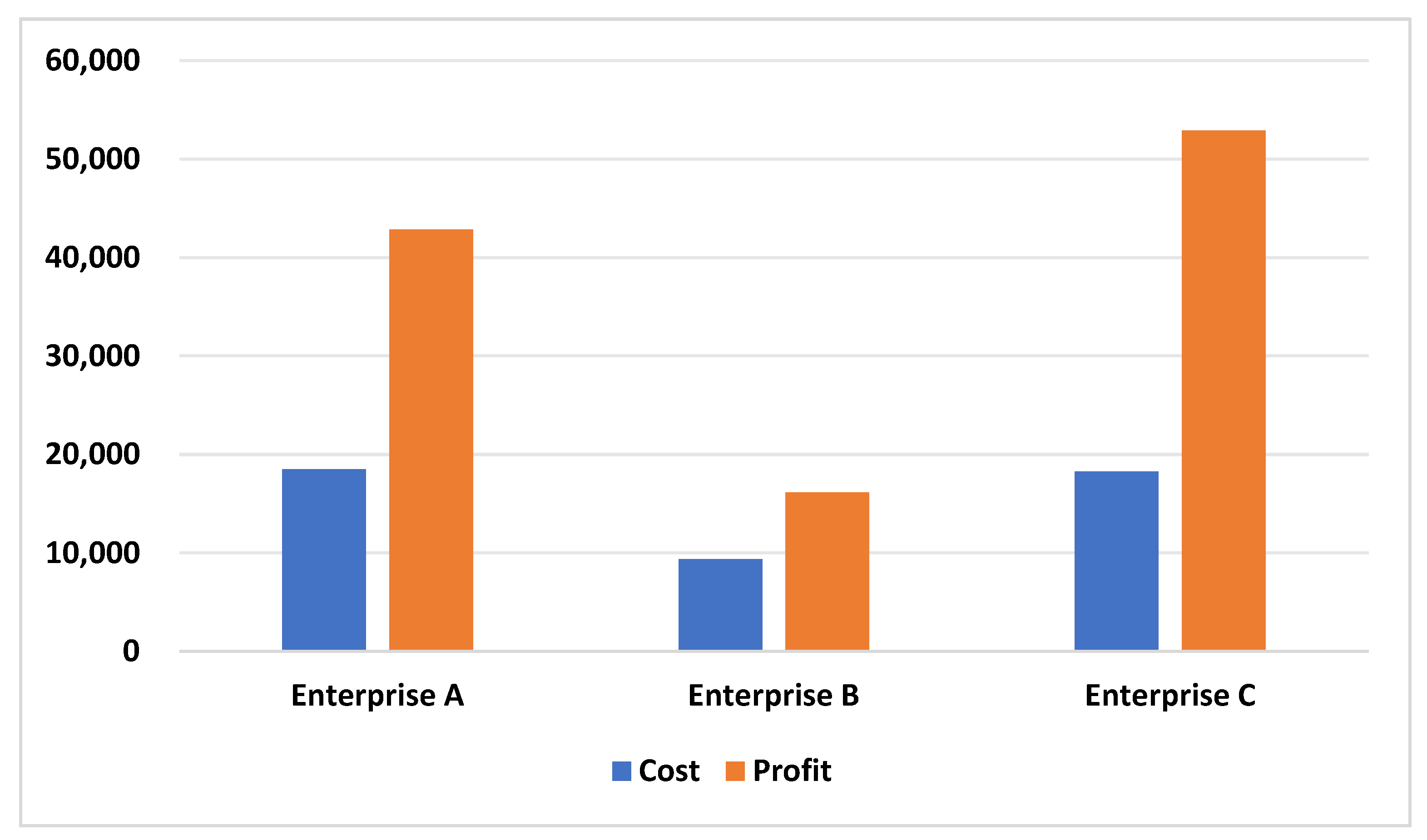
The equal division contribution value of a trapezoidal fuzzy number is allocated based on the contributions made by players after participating in the coalition. However, in practical cooperative games, we still need to take more situations into account. For instance, some enterprises, due to their own positive brand effects, still expand the influence of the coalition even if they do not make too many actual contributions after joining the coalition. In order to not ignore the potential value brought by these enterprises, we need to introduce player weights.
The weighted equal division contribution value of the trapezoidal fuzzy number also aims at minimizing the overall dissatisfaction of players. Therefore, the following quadratic programming model is established.
Problem 2.
min i N 1 ω ( i ) i N ( 1 ω ( i ) ) ( ( v L ( N ) v L ( N ˜ i ) x L β ω ( i ) ) 2 + ( v m 1 ( N ) v m 1 ( N ˜ i ) x m 1 β ω ( i ) ) 2 + ( v m 2 ( N ) v m 2 ( N ˜ i ) x m 2 β ω ( i ) ) 2 + ( v R ( N ) v R ( N ˜ i ) x R β ω ( i ) ) 2 ) s . t . i N x L β ω ( i ) = v L ( N ) i N x m 1 β ω ( i ) = v m 1 ( N ) i N x m 2 β ω ( i ) = v m 2 ( N ) i N x R β ω ( i ) = v R ( N ) .
The allocation strategy obtained by solving this model is called the weighted equal division contribution value of the trapezoidal fuzzy number. In Equation (12), ω ( i ) represents the player weight of player i in the coalition, while x L β ω ( i ) , x R β ω ( i ) , x m 1 β ω ( i ) , and x m 2 β ω ( i ) are respectively the lower limit value, the upper limit value, the left mean value, and the right mean value of the trapezoidal fuzzy number profit values allocated to the players after participating in the coalition.
The non-fuzzy weighted value is also only a precise number; it is
min i N 1 ω ( i ) i N ( 1 ω ( i ) ) ( v ( N ) v ( N ˜ i ) x β ω ( i ) ) 2 s . t . i N x L β ω ( i ) = v L ( N ) .
For the purpose of simplifying the Equation (12), we use ω * ( i ) to represent 1 ω ( i ) i N ( 1 ω ( i ) ) . As a result, Equation (12) can be rewritten as follows.
Problem 3.
min i N ω * ( i ) ( ( v L ( N ) v L ( N ˜ i ) x L β ω ( i ) ) 2 + ( v m 1 ( N ) v m 1 ( N ˜ i ) x m 1 β ω ( i ) ) 2 + ( v m 2 ( N ) v m 2 ( N ˜ i ) x m 2 β ω ( i ) ) 2 + ( v R ( N ) v R ( N ˜ i ) x R β ω ( i ) ) 2 ) s . t . i N x L β ω ( i ) = v L ( N ) i N x m 1 β ω ( i ) = v m 1 ( N ) i N x m 2 β ω ( i ) = v m 2 ( N ) i N x R β ω ( i ) = v R ( N ) .
The calculation process for the weighted equal division contribution value of a trapezoidal fuzzy number is similar to that for the unweighted value. The detailed phases will be introduced.
Phase 1.
We construct the Lagrange function of Equation (13), and we obtain
L ( x β ω , λ β ω , μ β ω , θ β ω , ρ β ω ) = i N ω * ( i ) ( v L ( N ) v L ( N ˜ i ) x L β ω ( i ) ) 2 + i N ω * ( i ) ( v m 1 ( N ) v m 1 ( N ˜ i ) x m 1 β ω ( i ) ) 2 + i N ω * ( i ) ( v m 2 ( N ) v m 2 ( N ˜ i ) x L β ω ( i ) ) 2 + i N ω * ( i ) ( v R ( N ) v R ( N ˜ i ) x R β ω ( i ) ) 2 + λ β ω ( i N x L β ω ( i ) v L ( N ) ) + μ β ω ( i N x m 1 β ω ( i ) v m 1 ( N ) ) + θ β ω ( i N x m 2 β ω ( i ) v m 2 ( N ) ) + ρ β ω ( i N x R β ω ( i ) v R ( N ) ) .
According to Equation (14), we calculate the partial derivatives of the function L ( x β ω ) with respect to x L β ω ( i ) , x m 1 β ω ( i ) , x m 2 β ω ( i ) , x R β ω ( i ) , λ β ω , μ β ω , θ β ω , and ρ β ω respectively, and set them all equal to 0. Then, we obtain
( L ) ( x L β ω ( i ) ) = 2 ω * ( i ) ( v L ( N ) v L ( N ˜ i ) x L β ( i ) ) + λ β ω * = 0 ( L ) ( x m 1 β ω ( i ) ) = 2 ω * ( i ) ( v m 1 ( N ) v m 1 ( N ˜ i ) x m 1 β ( i ) ) + μ β ω * = 0 ( L ) ( x m 2 β ω ( i ) ) = 2 ω * ( i ) ( v m 2 ( N ) v m 2 ( N ˜ i ) x m 2 β ( i ) ) + θ β ω * = 0 ( L ) ( x R β ω ( i ) ) = 2 ω * ( i ) ( v R ( N ) v R ( N ˜ i ) x R β ( i ) ) + ρ β ω * = 0 ( L ) ( λ β ω ) = i N x L β ω ( i ) v L ( N ) = 0 ( L ) ( μ β ω ) = i N x m 1 β ω ( i ) v m 1 ( N ) = 0 ( L ) ( θ β ω ) = i N x m 2 β ω ( i ) v m 2 ( N ) = 0 ( L ) ( ρ β ω ) = i N x R β ω ( i ) v R ( N ) = 0 .
In Equation (15), λ β ω * , μ β ω * , θ β ω * , and ρ β ω * respectively represent the remainder terms obtained by taking the partial derivatives of the independent variables x L β ω ( i ) , x m 1 β ω ( i ) , x m 2 β ω ( i ) , and x R β ω ( i ) with respect to Equation (14).
Phase 2.
We take the lower limit value x L β ω ( i ) of the weighted equal division contribution value of the trapezoidal fuzzy number as an example and continue to calculate its solution.
Based on Equation (15), we can obtain
x L β ω ( i ) = v L ( N ) v L ( N ˜ i ) λ β ω * 2 ω * ( i ) .
According to Equations (15) and (16), we can observe
i N x L β ω ( i ) = n v L ( N ) j N v L ( N ˜ j ) λ β ω * j N 1 2 ω * ( j ) = v L ( N ) .
By rewriting Equation (17) into another form, we obtain
λ β ω * = ( n 1 ) v L ( N ) j N v L ( N ˜ j ) j N 1 2 ω * ( j ) .
Suppose v β ( i ) denotes the contribution value of player i to the coalition. By substituting Equation (9) into Equation (7), the lower limit value of the weighted equal division contribution value of the trapezoidal fuzzy number can be obtained as
x L β ω ( i ) = v L ( N ) v L ( N ˜ i ) ( n 1 ) v L ( N ) j N v L ( N ˜ j ) ω * ( i ) j N 1 ω * ( j ) = v L β ( i ) + v L ( N ) j N v L β ( j ) ω * ( i ) j N 1 ω * ( j ) .
Phase 3.
We apply the process of deriving the lower limit value x L β ω ( i ) to calculate the upper limit value x R β ω ( i ) , the left mean value x m 1 β ω ( i ) , and the right mean value x m 2 β ω ( i ) of the weighted equal division contribution value of the trapezoidal fuzzy number. It can thus be seen that if the sum of the contributions made by players is less than the coalition’s profit, the weighted equal division contribution value of the trapezoidal fuzzy number x β ω ( i ) is
x β ω ( i ) = [ x L β ω ( i ) , x m 1 β ω ( i ) , x m 2 β ω ( i ) , x R β ω ( i ) ] = [ v L β ( i ) + v L ( N ) j N v L β ( j ) ω * ( i ) j N 1 ω * ( j ) , v m 1 β ( i ) + v m 1 ( N ) j N v m 1 β ( j ) ω * ( i ) j N 1 ω * ( j ) , v m 2 β ( i ) + v m 2 ( N ) j N v m 2 β ( j ) ω * ( i ) j N 1 ω * ( j ) , v R β ( i ) + v R ( N ) j N v R β ( j ) ω * ( i ) j N 1 ω * ( j ) ] .
If the sum of the contributions made by players is more than the coalition’s profit, the weighted equal division contribution value of the trapezoidal fuzzy number x β ω ( i ) is
x β ω ( i ) = [ x L β ω ( i ) , x m 1 β ω ( i ) , x m 2 β ω ( i ) , x R β ω ( i ) ] = [ v L β ( i ) + v L ( N ) j N v L β ( j ) ω ( i ) j N 1 ω ( j ) , v m 1 β ( i ) + v m 1 ( N ) j N v m 1 β ( j ) ω ( i ) j N 1 ω ( j ) , v m 2 β ( i ) + v m 2 ( N ) j N v m 2 β ( j ) ω ( i ) j N 1 ω ( j ) , v R β ( i ) + v R ( N ) j N v R β ( j ) ω ( i ) j N 1 ω ( j ) ] .
Different from this solution, the non-fuzzy weighted equal division contribution is
x β ω ( i ) = v β ( i ) + v ( N ) j N v β ( j ) ω ( i ) j N 1 ω ( j ) .
Obviously, like the unweighted value, the non-fuzzy weighted equal division contribution value struggles to cope with the effects arising from changes in the game environment.

4.3. Some Properties of the Solution

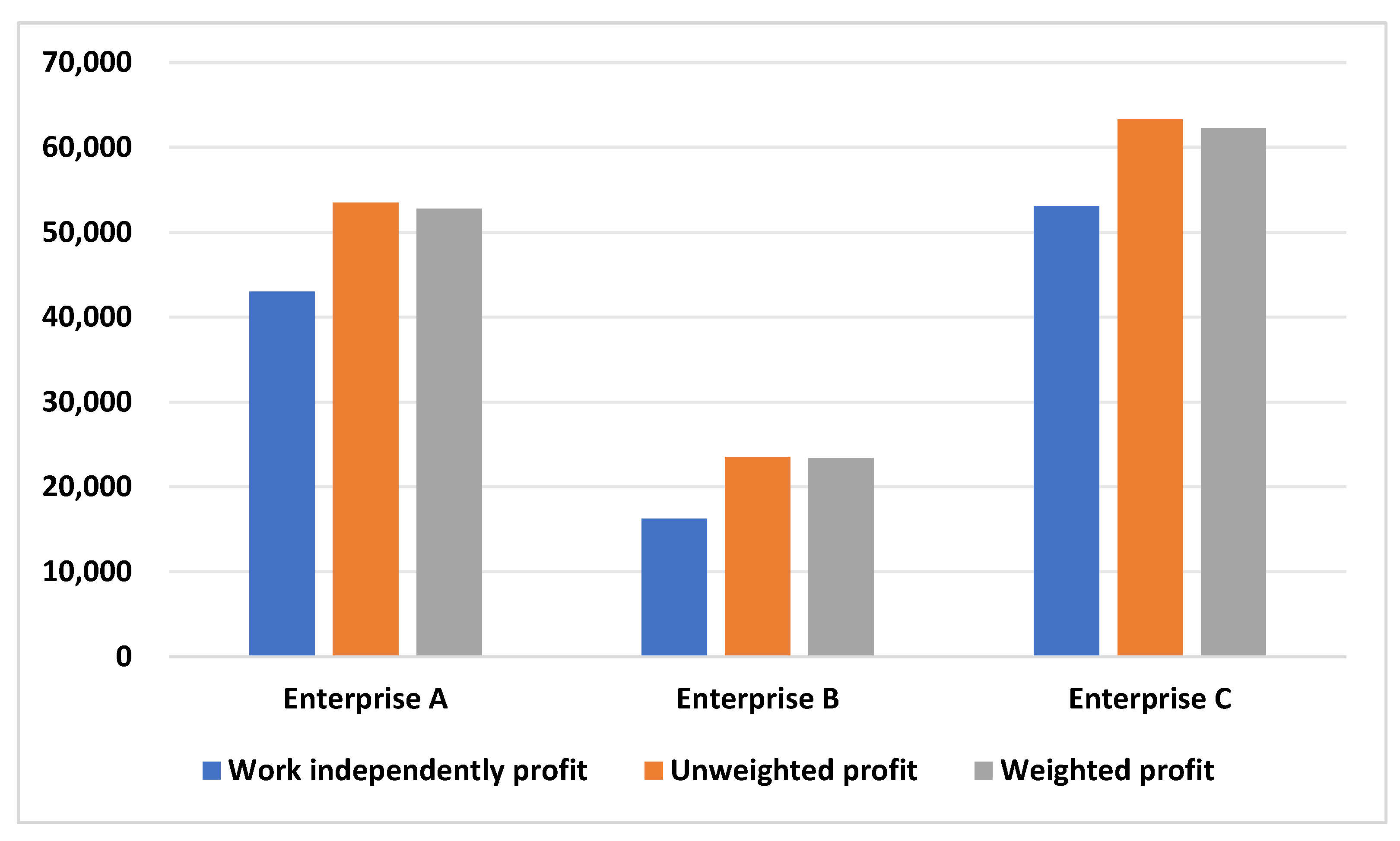
Since the unweighted equal division contribution value of the trapezoidal fuzzy number and the weighted value have the same properties, only the unweighted equal division contribution value of the trapezoidal fuzzy number is taken as an example here, and the properties of the weighted value will not be elaborated on any further.
Theorem 1.
(Validity) Let P n  denote the set of cooperative games with n  players. For any trapezoidal fuzzy number cooperative game v P n ,after applying the equal division contribution value of the trapezoidal fuzzy number as the allocation strategy, all players i N  can exactly divide up the profit v ( N )  of the grand coalition N .
Proof of Theorem 1.
According to the addition operation rule of the trapezoidal fuzzy number, we can obtain
i = 1 n x β ( i ) = [ i = 1 n x L β ( i ) , i = 1 n x m 1 β ( i ) , i = 1 n x m 2 β ( i ) , i = 1 n x R β ( i ) ] = [ v L ( N ) + j N v L ( N ˜ j ) i = 1 n v L ( N ˜ i ) , v m 1 ( N ) + j N v m 1 ( N ˜ j ) i = 1 n v m 1 ( N ˜ i ) ,     v m 2 ( N ) + j N v m 2 ( N ˜ j ) i = 1 n v m 2 ( N ˜ i ) , v R ( N ) + j N v R ( N ˜ j ) i = 1 n v R ( N ˜ i ) ] = [ v L ( N ) , v m 1 ( N ) , v m 2 ( N ) , v R ( N ) ] .
It can be determined from Equation (22) that i = 1 n x β ( i ) = v ( N ) , which indicates that the sum of the profit values allocated to all players i N from the grand coalition N is exactly the coalition profit v ( N ) . Therefore, all players can exactly divide up the total profit of the grand coalition.
Theorem 2.
(Additivity) Let P n  denote the set of cooperative games with n  players. For any cooperative games v P n  and u P n with equal division contribution values of the trapezoidal fuzzy numbers, it always holds that x β ( v + u ) = x β ( v ) + x β ( u )
Proof of Theorem 2.
According to Equation (10) and the addition operation rule of trapezoidal fuzzy numbers, we can obtain
x L β ( v + u ) = v L ( N ) + u L ( N ) + j N v L ( N ˜ j ) + j N u L ( N ˜ j ) n v L ( N ˜ i ) u L ( N ˜ i ) = v L ( N ) + j N v L ( N ˜ j ) n v L ( N ˜ i ) + u L ( N ) + j N u L ( N ˜ j ) n u L ( N ˜ i ) = x L β ( v ) + x L β ( u ) .
Through the same method, other values can be calculated as
x m 1 β ( v + u ) = x m 1 β ( v ) + x m 1 β ( u ) x m 2 β ( v + u ) = x m 2 β ( v ) + x m 2 β ( u ) x R β ( v + u ) = x R β ( v ) + x R β ( u ) .
Therefore, we can obtain x β ( v + u ) = x β ( v ) + x β ( u ) .
Theorem 3.
(Symmetry) Let P n denote the set of cooperative games with n  players. If any two players i N  and h N ( i h )   in the cooperative game v P n  with an equal division contribution value of the trapezoidal fuzzy number have equal status within the coalition, then the allocated profit value x β ( i ) = x β ( h ) .
Proof of Theorem 3.
According to Equation (10), for players i N  and h N ( i h )   with the same status, it holds that
x L β ( i ) = v L ( N ) + j N v L ( N ˜ j ) n v L ( N ˜ i ) x L β ( h ) = v L ( N ) + j N v L ( N ˜ j ) n v L ( N ˜ h ) .
If players i and h have equal status within the coalition, it indicates that v L ( N ˜ i ) = v L ( N ˜ h ) , and then x L β ( i ) = x L β ( h ) also holds. Through a similar method, we can obtain
x m 1 β ( i ) = x m 1 β ( h ) x m 2 β ( i ) = x m 2 β ( h ) x R β ( i ) = x R β ( h ) .
According to the operation rule of trapezoidal fuzzy number, it can be known that x β ( i ) = x β ( h ) .

5. Analysis of the Practical Case

5.1. Background

5.1.1. Basic Information of the Case

A “full load” generally encompasses both a full load in terms of weight and a full load in terms of volume, and both of these are significant issues that require close attention during transportation. Components of general road freight are usually complex and diverse, including high-density items such as steel bars and bricks. As a result, transport vehicles may reach full load in terms of both volume and weight. However, agricultural product cold chain transportation differs from general road freight. Given that the unit weight of the goods transported is relatively small, it is more likely to reach full-load volume rather than full-load weight under normal circumstances. Based on this fact, we study the following case.
There are three agricultural product cold chain logistics enterprises planning to transport fresh lettuce from Changsha to Shenzhen. Since the leaves of the lettuce are delicate, crisp, tender, and contain a lot of water, its volume per unit mass is relatively large, and its density is relatively low. Based on this characteristic, with the goal of making the volume of transport vehicles as fully loaded as possible to save transport vehicles, we establish a coalition of agricultural product cold chain transportation enterprises through the combination of orders.
We have presented the operation mode of the coalition in a simple and intuitive way in Figure 1.

5.1.2. Analysis of Relevant Parameters

After conducting on-site investigations of the enterprises, this paper lists the following parameters that are of reference significance.
(1)
Distance D (unit: km). This refers to the distance between the starting point and the ending point.
(2)
Fuel cost F (unit: CNY/km). This refers to the fuel cost consumed per kilometer during the transportation process of a single vehicle. Affected by the market price of fuel, its value usually fluctuates within a certain range.
(3)
Expressway toll E (unit: CNY/t/km). This refers to the cost incurred when a single vehicle travels on the expressway during the transportation process.
(4)
Number of vehicle departures per year n (unit: times). This refers to the total number of outbound trips of the vehicle on this route in a year. Affected by weather, road conditions, and the number of orders, its value fluctuates within a certain range.
(5)
Annual insurance cost I (unit: CNY). This refers to the vehicle insurance cost that is paid for a single vehicle each year.
(6)
Annual maintenance and repair cost M (unit: CNY). This refers to the maintenance and repair cost that is paid for a single vehicle each year.
(7)
Annual salary of drivers S d (unit: CNY). This refers to the salaries paid by the enterprise to drivers each year. Since transportation tasks usually take a long time, in order to ensure the safety of drivers, generally two drivers are required for a single vehicle to complete one transportation task.
(8)
Annual salary of managers S m (unit: CNY). This refers to the salaries paid by the enterprise to managers each year. S m = 0.1 S d .
(9)
Annual risk cost O (unit: CNY). This refers to the potential cost of wasted transportation capacity when vehicles return empty.
(10)
Initial vehicle purchase cost P (unit: CNY). This refers to the cost required for an enterprise to purchase a single vehicle.
(11)
Equipment depreciation cost Q (unit: CNY). The depreciation period is set as 5 years, and the depreciation expense Q = P 5 n .
(12)
Loading and unloading service cost L (unit: CNY/m). This refers to the cost of labor and equipment required for loading and unloading vehicles.
(13)
Vehicle volume V (unit: m3).
(14)
Volume of goods G (unit: m3).
(15)
Density of goods W (unit: t/m3).
(16)
Weight of the vehicle L (unit: t).
(17)
Vehicle loading rate δ . This represents the full-load level of agricultural products transported by a single cold chain transport vehicle. The higher the full-load level is, the greater the vehicle loading rate will be. The vehicle loading rate δ = G V .
(18)
Penalty coefficient τ . If the vehicle is not fully loaded, it is likely to result in wasted trips and a loss of opportunities. Therefore, in order to encourage transport vehicles to be as close to a full load as possible, a penalty coefficient is introduced here. The lower the loading rate is, the higher the penalty coefficient will be, and the greater the penalty cost will be. The penalty coefficient τ = 1 + 1 δ 4 .
Based on the above parameters, the cost C (unit: CNY) for a single cold chain transport vehicle for agricultural products to complete one transportation task can be obtained as
C = [ D F + D E ( G Z + W ) + Q + L G + I + M + 2 S d + S m + O n ] τ .
If the order quotation is K (unit: CNY), then the profit v ( N ) of the coalition is
v ( N ) = K C = K [ D F + D E ( G Z + W ) + Q + L G + I + M + 2 S d + S m + O n ] τ .
Based on the results of on-site investigations of enterprises, we have listed the reference values of relevant parameters in Table 1.
Based on the above parameters and their corresponding reference values, in order to facilitate the subsequent calculations of profit and allocation, the following five assumptions and explanations are needed [34].
(1)
It is assumed that the equipment conditions and the technologies of the three cold chain logistics enterprises are advanced enough so that during the transportation process, there is no situation where the agricultural products undergo deterioration due to temperature change, and the damage rate of products is zero.
(2)
It is assumed that the operating conditions of the three cold chain logistics enterprises are similar, and all the relevant data shown in Table 1 for the three enterprises are the same.
(3)
The density of lettuce is calculated at 0.2 t/m3. Even if a 9.6 m cold chain transport vehicle is fully loaded, it only weighs 12 t, which is far below the rated load capacity of 17.2 t. Therefore, the calculations in this section do not involve overweight issues.
(4)
There is sufficiently tacit understanding among enterprises, and the formation of a coalition will not affect the quotations of the original orders.
(5)
After the enterprises form a coalition, the orders will be combined, and the volume errors of loading agricultural products after order combination will be ignored.

5.2. Calculating the Profit of the Coalition

5.2.1. Calculating the Costs and Profits of a Single Enterprise

The three cold chain logistics enterprises in the case are represented by enterprise A, enterprise B, and enterprise C. For the convenience of calculation, the specification of the lettuce to be transported will be changed from the common weight specification to the volume specification after being packaged uniformly.
In this case, the transportation order information of the three enterprises is summarized in Table 2 and includes the volume of lettuce to be transported and the order quotations.
Affected by seasons and harvest conditions, the price of lettuce fluctuates within a certain range. Representing the order quotations with trapezoidal fuzzy numbers can better conform to this real situation. The maximum volume of a 9.6 m cold chain transport vehicle is 60 m3. Therefore, if the three enterprises work independently, enterprise A, enterprise B, and enterprise C will need to mobilize two, one, and two transport vehicles, respectively.
Let the weight of the lettuce in a single cold chain transport vehicle be L G . When enterprise A works independently, among the two cold chain transport vehicles it mobilizes, one vehicle J A 1 is fully loaded, where the vehicle loading rate δ = 100 % and the weight of the goods L G = 12 t . For the other vehicle J A 2 , the loading rate δ = G V = 10 60 = 16.67 % and the weight of the goods L G = 12 × δ = 12 × 1 6 = 2 t .
By using the same method, we can also calculate the vehicle usage information of enterprise B and enterprise C and summarize it, as shown in Table 3.
According to Table 1 and Table 2 and Equation (27), we can calculate the transportation costs of enterprises when they operate independently.
For enterprise A, the lower limit value C L A of the transportation cost is the sum of the lower limit values of the transportation costs of the two vehicles, that is, C L A = C L A 1 + C L A 2 . Among them, the lower limit value of the transportation costs of the vehicles J A 1 and J A 2 are
C L A 1 = [ D F + D E ( G Z + W ) + Q + L G + I + M + 2 S d + S m + O n ] τ = [ 960 × 5.53 + 960 × 0.037 ( 60 × 0.2 + 30 ) + 400,000 160 × 5 + 3 × 60 + 14,400 + 840 + 210,000 + 500 160 ] × 1 = 8891.52
C L A 2 = [ D F + D E ( G Z + W ) + Q + L G + I + M + 2 S d + S m + O n ] τ = [ 960 × 5.53 + 960 × 0.037 ( 60 × 0.2 + 30 ) + 400,000 160 × 5 + 3 × 10 + 14,400 + 840 + 210,000 + 500 160 ] × 29 24 = 10,133.46
Therefore, the lower limit value C L A of the transportation cost of enterprise A is C L A = C L A 1 + C L A 2 = 19,024.98 .
In the same way, it can be calculated that
C m 1 A = 21,692.01 C m 2 A = 23,394.44 C R A = 26,132.71 .
Through the above calculations, we obtain all the key values of the trapezoidal fuzzy numbers for cost. As a result, the transportation cost of enterprise A is C A = [ 19,024.98 , 21,692.01 , 23,394.44 , 26,132.71 ] . Then, we subtract the cost from the order quotation, and we obtain v A = K A C A = [ 42,267.29 , 45,205.56 , 47,057.99 , 49,975.03 ] .
Similarly, we can calculate the costs and profits of enterprise B and enterprise C. We list all these values in Table 4. To visualize the data, we show the lower limit values of cost and profit in Figure 2.

5.2.2. Calculating the Costs and Profits of the Coalition

For enterprise A and enterprise B, after they form a coalition, the transportation volume of the orders undertaken by the coalition increases, and a total of 100 m3 of lettuce needs to be transported. At this time, for the coalition formed by enterprise A and enterprise B (hereinafter referred to as coalition AB for short, and the abbreviations of other coalitions are similar), a total of two 9.6 m cold chain transport vehicles are required to complete the combined orders.
Among them, one vehicle J A B 1 is fully loaded, were the vehicle loading rate δ = 100 % and the weight of the goods L G = 12 t . The loading rate of the other vehicle J A B 2 is δ = G V = 40 60 = 66.67 % , and the weight of the goods L G = 12 × δ = 12 × 2 3 = 8 t .
By using the same method, we can also calculate the vehicle usage information of all coalitions and summarize it, as shown in Table 5.
For coalition AB, the lower limit value C L A B of the transportation cost is the sum of the lower limit values of the transportation costs of the two vehicles, that is, C L A B = C L A B 1 + C L A B 2 . Among them, the lower limit value of the transportation costs of the vehicles J A B 1 and J A B 2 are
C L A B 1 = [ D F + D E ( G Z + W ) + Q + L G + I + M + 2 S d + S m + O n ] τ = [ 960 × 5.53 + 960 × 0.037 ( 60 × 0.2 + 30 ) + 400,000 160 × 5 + 3 × 60 + 14,400 + 840 + 210,000 + 500 160 ] × 1 = 8891.52
C L A B 2 = [ D F + D E ( G Z + W ) + Q + L G + I + M + 2 S d + S m + O n ] τ = [ 960 × 5.53 + 960 × 0.037 ( 60 × 0.2 + 30 ) + 400,000 160 × 5 + 3 × 40 + 14,400 + 840 + 210,000 + 500 160 ] × 13 12 = 9413.56
Therefore, the lower limit value C L A B of the transportation cost of coalition AB is C L A B = C L A B 1 + C L A B 2 = 18,305.07 .
In the same way, it can be calculated that
C m 1 A B = 20,821.14 C m 2 A B = 22,427.21 C R A B = 25,010.47 .
Through the above calculations, we obtain all the key values of the trapezoidal fuzzy numbers for cost. As a result, the transportation cost of coalition AB is C A B = [ 18,305.07 ,   20,821.14 ,   22,427.21 ,   25,010.47 ] . Then, we subtract the cost from the order quotation, and we obtain v A B = K A + K B C A B = [ 72,539.53 ,   75,572.79 ,   77,728.86 ,   80,694.93 ] .
Similarly, we can calculate the costs and profits of the other coalitions. We list all these values in Table 6.
As can be seen from Table 4 and Table 6, after enterprise A and enterprise B form coalition AB, their cooperative profit v A B = [ 72,539.53 ,   75,572.79 ,   77,728.86 ,   80,694.93 ] . The sum of the profit when they work independently v A + v B = [ 59,023.33 ,   63,589.12 ,   66,686.62 ,   71,146.41 ] . Therefore, the profit v A B > v A + v B after enterprise A and B form a coalition, which satisfies the super-additivity of the cooperative game and is the motivation for enterprise A and enterprise B to form a coalition. Similarly, the relationships between the profits of other coalitions and the sum of the profits when the players work independently can be obtained and are listed in Table 7.
As can be seen from Table 6 and Table 7, the cooperative profits of the enterprise coalitions AB, AC, and BC are all greater than the sum of the profits of the enterprises participating in the coalitions when they operate independently. Therefore, any two of these three enterprises have the motivation to form a coalition with each other. In addition, the sum of the profits of coalition AB and enterprise C when operating independently, the sum of the profits of coalition AC and enterprise B when operating independently, and the sum of the profits of coalition BC and enterprise A when operating independently are all less than the profit when enterprises A, B, and C form coalition ABC. Consequently, enterprises A, B, and C are more inclined to form the large tripartite cooperative coalition ABC.

5.3. Profit Allocation Strategy

Let the weights of the players be ( ω ( A ) , ω ( B ) , ω ( C ) ) = ( 3 12 , 4 12 , 5 12 ) . Now take x β ( A ) as an example to calculate the profit allocation strategy for the unweighted equal division contribution value of the trapezoidal fuzzy number.
For enterprise A, its contribution value to coalition ABC is v β ( A ) . Through calculation, we obtain v β ( A ) = v A B C v B C = [ 48,767.93 ,   55,953.59 ,   61,090.26 ,   68,295.01 ] . Similarly, we can obtain the value v β ( B ) = [ 19,164.64 ,   27,708.66 ,   33,430.49 ,   41,928.54 ] and the value v β ( C ) = [ 58,624.74 ,   65,910.72 ,   71,079.52 ,   78,385.93 ] .
According to Equation (10), we can obtain the lower limit value x L β ( A ) of the profit allocated to enterprise A.
x L β ( A ) = v L β ( A ) + v L ( N ) j N v L β ( j ) n = 48,767.93 + 139,319.67 ( 48,767.93 + 19,164.64 + 58,624.74 ) 3 = 53,022.05 .
In this way, we can calculate the profits of enterprise A, B, and C respectively.
x β ( A ) = [ 53,022.05 ,   53,975.79 ,   54,774.27 ,   55,733.67 ] , x β ( B ) = [ 23,418.76 ,   25,730.86 ,   27,114.50 ,   29,367.20 ] , x β ( C ) = [ 62,878.86 ,   63,932.92 ,   64,763.53 ,   65,824.59 ] .
Next, taking x β ω ( A ) as an example, we calculate the weighted equal division contribution value of the trapezoidal fuzzy number. After observation, it is found that the sum of the lower limit values of the contributions made by enterprise A, enterprise B, and enterprise C is less than the lower limit value of the profit of coalition ABC, and the sum of the left mean values of the contributions made by enterprise A, enterprise B, and enterprise C is greater than the left mean value of the profit of coalition ABC. Therefore, according to Equations (19)–(21), we obtain
x L β ω ( A ) = v L β ( A ) + v L ( N ) j N v L β ( j ) ω * ( A ) i N 1 ω * ( i ) = 48,767.93 + 1,439,319.67 ( 48,767.93 + 19,164.64 + 58,624.74 ) 3 8 × ( 8 3 + 3 + 24 7 ) = 52,509.77
x m 1 β ω ( A ) = v m 1 β ( A ) + v m 1 ( N ) j N v m 1 β ( j ) ω ( A ) i N 1 ω ( i ) = 55,953.59 + 143,639.58 ( 55,953.59 + 27,708.66 + 65,910.72 ) 3 12 × ( 12 3 + 12 4 + 12 5 ) = 53,428.74
In this way, we can calculate the profits of enterprise A, B, and C.
x β ω ( A ) = [ 52,259.26 ,   52,509.77 ,   53,027.30 ,   53,428.74 ] , x β ω ( B ) = [ 22,906.48 ,   25,183.81 ,   25,367.53 ,   25,892.79 ] , x β ω ( C ) = [ 62,350.18 ,   62,366.58 ,   63,016.56 ,   63,385.87 ] .

5.4. Strategy Comparison and Analysis

We list the profits when the players work independently and the unweighted and weighted equal division contribution values of the trapezoidal fuzzy numbers in Table 8, and we also list the results using non-fuzzy strategies in Table 9.
In order to display the data in Table 8 more intuitively, taking the lower limit values of the profit of each enterprise in Table 8 as an example, we draw Figure 3.
It can be seen from Table 8 and Figure 3 that the profit of enterprise C is always the highest among the three enterprises, while the allocated profit of enterprise B is always the lowest. According to the profit of the players when working independently in Table 4 and the calculation of the players’ contributions in Section 5.3, it can be found that there is always a relationship of “enterprise C > enterprise A > enterprise B” among the profits obtained when working independently and the contribution values. The allocation results presented in Table 8 precisely illustrate that after enterprises participate in the coalition, the allocated profit is positively correlated with the profits obtained when working independently and the contributions to the coalition.
When considering the situation of weights, for enterprise C with the largest weight, after adopting the weighted allocation strategy, its allocated profit increases, while for enterprise A with the smallest weight, its allocated profit decreases. The weight of enterprise B is 4/12, which is exactly 1/3. Therefore, within the tripartite cooperative enterprise coalition, enterprise B is the least affected by the weighted allocation strategy compared with the situation when weights are not considered. Consequently, the introduced profit allocation strategy with weights is more beneficial to the enterprises that play a dominant role in the coalition.
On the other hand, compared with the non-fuzzy equal division contribution value solution using precise numbers, the solution proposed in this paper, which uses trapezoidal fuzzy numbers, can better reflect the complex and changeable practical game environment. As a result, it is more valuable for coalitions and enterprises.
Generally speaking, the equal division contribution value of the trapezoidal fuzzy number not only features the fairness and reasonableness of the equal division contribution value but can also cope well with the impact on the allocation strategy when the game environment changes.

6. Conclusions

Today, with the rapid development of the agricultural product cold chain logistics industry, practitioners in the industry are still faced with problems such as the waste of transportation capacity resources, low vehicle loading rates, and high transportation costs. Especially for small and medium-sized enterprises, it is difficult to withstand risks in such an operating environment.
To break through this dilemma, first of all, this paper studies and puts forward a method for constructing a coalition of agricultural product cold chain logistics enterprises. With the goal of minimizing the overall dissatisfaction of the players, a mathematical model of the equal division contribution value of the trapezoidal fuzzy number is established, and solutions are calculated. Second, by combining the orders of different enterprises, the vehicle loading rate in the transportation stage can be increased or the number of required transport vehicles can be reduced, so as to achieve the purpose of reducing costs and increasing efficiency. Third, taking the equal division contribution value of the trapezoidal fuzzy number as the allocation strategy for the coalition’s profit, profits are allocated to each player, and a comparative analysis of different strategies is carried out. Finally, a conclusion is obtained that using the enterprise coalition method proposed in this paper with the equal division contribution value of the trapezoidal fuzzy number as the profit allocation strategy can effectively increase the profit of enterprises while ensuring fairness and reasonableness. Moreover, this strategy can effectively deal with the impact of changes in values due to changes in the game environment.
There are some limitations to the research presented in this paper. For example, this study takes a relatively objective perspective and uses the square contribution excess as a measure to evaluate the dissatisfaction of the players. However, in practical applications, decision-makers in enterprises often find it difficult to be completely rational. Their satisfaction with the allocation results may also change according to the actual needs of the enterprise, and there are many factors that cannot be measured by data.
Theoretically speaking, the method in this paper is not limited to agricultural products such as lettuce. For future research, all coalitions that can achieve enterprise cooperation through the order combination method can apply the allocation strategy using the equal division contribution value of the trapezoidal fuzzy number proposed in this paper to achieve the purpose of reducing costs and increasing efficiency. The model of the equal division contribution value of the trapezoidal fuzzy number constructed in this paper can be widely applied to the problem of cooperative game profit allocation in various fuzzy environments according to the actual needs of the coalition and can put forward reasonable and reliable solutions.

Author Contributions

Conceptualization, J.Z.; methodology, J.Z. and J.L.; investigation, J.Z., R.F. and M.L.; writing—original draft, J.Z.; writing—review & editing, J.Z. and R.F.; visualization, J.L. and W.Z.; supervision, J.L. and W.Z. All authors have read and agreed to the published version of the manuscript.

Funding

This work was supported by the National Social Science Foundation of China (22BGL005), the Guiding Project of Fujian Science and Technology Program (2021N0007), the Post-funded General Project of the Ministry of Education in the Philosophy and Social Science (23JHQ095), the Research Project of the Philosophy and Social Science of the Education System in Fujian Province (JAS24213), and the Open Project of Xi Jinping Thought on Ecological Civilization Research Institute of Fujian Agriculture and Forestry University (STWMSX23-15).

Data Availability Statement

The original contributions presented in this study are included in the article.

Conflicts of Interest

The authors declare no conflicts of interest.

References

  1. Mottaghi, A.; Ezzati, R.; Khorram, E. A new method for solving fuzzy linear programming problems based on the fuzzy linear complementary problem (FLCP). Int. J. Fuzzy Syst. 2015, 17, 236–245. [Google Scholar] [CrossRef]
  2. Zhang, H.D.; Shu, L. Generalized interval-valued fuzzy rough set and its application in decision making. Int. J. Fuzzy Syst. 2015, 17, 279–291. [Google Scholar] [CrossRef]
  3. Montanari, R. Cold chain tracking: A managerial perspective. Trends Food Sci. Technol. 2008, 19, 425–431. [Google Scholar] [CrossRef]
  4. Ren, J.J.; Li, H.X.; Zhang, M.M.; Wu, C.; Yu, X.S. A self-powered sensor network data acquisition, modeling and analysis method for cold chain logistics quality perception. IEEE Sens. J. 2023, 23, 20729–20736. [Google Scholar] [CrossRef]
  5. Wang, X.; Xia, J.; Zou, J.; Hung, W.; Matetic, M.; Bakarić, M.B.; Zhang, X. Pathways toward precise monitoring and low-carbon sustainability in fruit cold chain logistics: A solution enabled by flexible temperature sensing. Mater. Today Sustain. 2023, 24, 100592. [Google Scholar]
  6. Huang, W.T.; Wang, X.P.; Zhang, J.C.; Xia, J.; Zhang, X.S. Improvement of blueberry freshness prediction based on machine learning and multi-source sensing in the cold chain logistics. Food Control 2023, 145, 109496. [Google Scholar] [CrossRef]
  7. Xiao, X.Q.; He, Q.L.; Fu, Z.T.; Xu, M.; Zhang, X.S. Applying CS and WSN methods for improving efficiency of frozen and chilled aquatic products monitoring system in cold chain logistics. Food Control 2016, 60, 656–666. [Google Scholar] [CrossRef]
  8. Huang, W.T.; Xia, J.; Wang, Y.F.; Jin, X.Y.; Zhu, H.L.; Zhang, X.S. Flexible multimode sensors based on hierarchical microstructures enable non-destructive grading of fruits in cold chain logistics. Mater. Today Sustain. 2024, 25, 100691. [Google Scholar] [CrossRef]
  9. Zhao, L.; Yu, Q.F.; Li, M.; Wang, Y.F.; Li, G.L.; Sun, S.N.; Fan, J.; Liu, Y.L. A review of the innovative application of phase change materials to cold-chain logistics for agricultural product storage. J. Mol. Liq. 2022, 365, 120088. [Google Scholar] [CrossRef]
  10. Bai, B.; Chen, N.; Li, X.Z. Application research of nano-storage materials in cold chain logistics of e-commerce fresh agricultural products. Res. Phys. 2019, 13, 102049. [Google Scholar] [CrossRef]
  11. Meng, B.B.; Zhang, X.L.; Hua, W.S.; Liu, L.; Ma, K.L. Development and application of phase change material in fresh e-commerce cold chain logistics: A review. J. Energy Storage 2022, 55, 105373. [Google Scholar] [CrossRef]
  12. Guan, X.M.; Li, G.P. Optimization of cold chain logistics vehicle transportation and distribution model based on improved ant colony algorithm. Procedia Comput. Sci. 2023, 228, 974–982. [Google Scholar] [CrossRef]
  13. Zhao, B.L.; Gui, H.X.; Li, H.Z.; Xue, J. Cold chain logistics path optimization via improved multi-objective ant colony algorithm. IEEE Access 2020, 8, 142977–142995. [Google Scholar] [CrossRef]
  14. Wu, L.J.; Shi, L.; Zhan, Z.H.; Lai, K.K.; Zhang, J. A buffer-based ant colony system approach for dynamic cold chain logistics scheduling. IEEE Trans. Emerg. Top. Comput. Intell. 2022, 6, 1438–1452. [Google Scholar] [CrossRef]
  15. Miao, X.H.; Pan, S.J.; Chen, L. Optimization of perishable agricultural products logistics distribution path based on IACO-time window constraint. Intell. Syst. Appl. 2023, 20, 200282. [Google Scholar] [CrossRef]
  16. Zhang, A.B.; Zhang, Y.; Liu, Y.Q. Low-carbon cold-chain logistics path optimization problem considering the influence of road impedance. IEEE Access 2023, 11, 124055–124067. [Google Scholar] [CrossRef]
  17. Yang, F.; Tao, F.M. A bi-objective optimization VRP model for cold chain logistics: Enhancing cost efficiency and customer satisfaction. IEEE Access 2023, 11, 127043–127056. [Google Scholar] [CrossRef]
  18. Lubenow, B.L.; Fairley, J.P.; Lindsey, C.R.; Larson, P.B. Cold supply chain logistics: System optimization for real-time rerouting transportation solutions. Comput. Ind. 2018, 95, 68–80. [Google Scholar]
  19. Zheng, F.; Zhou, X. Sustainable model of agricultural product logistics integration based on intelligent blockchain technology. Sustain. Energy Technol. Assess. 2023, 57, 103258. [Google Scholar] [CrossRef]
  20. Chamath, E.; Yapa, M.B.; Maxwell, C.; Prem, C. An order fulfilment location planning model for perishable goods supply chains using population density. Supply Chain. Anal. 2023, 4, 100045. [Google Scholar]
  21. Zhang, Y.D.; Fan, X.M.; Ma, Y.H.; Sun, Y.Q. Spatial impacts of cold chain logistics for fresh agri-products on carbon emissions. Trans. Res. Part D Transp. Environ. 2022, 113, 103525. [Google Scholar] [CrossRef]
  22. Liu, Z.; Huang, Y.Q.; Shang, W.L.; Zhao, Y.J.; Yang, Z.L.; Zhao, Z. Precooling energy and carbon emission reduction technology investment model in a fresh food cold chain based on a differential game. Appl. Energy 2022, 326, 119945. [Google Scholar] [CrossRef]
  23. Shapley, L.S. A Value for n-Person Games; Princeton University Press: Princeton, NJ, USA, 1953. [Google Scholar]
  24. Banzhaf, J.F., III. Weighted voting doesn’t work: A mathematical analysis. Rutgers Law Rev. 1965, 19, 317–343. [Google Scholar]
  25. Song, J.K.; Ma, X.P.; Chen, R. A profit distribution model of reverse logistics based on fuzzy DEA efficiency—Modified shapley value. Sustainability 2021, 13, 7354. [Google Scholar] [CrossRef]
  26. Manuel, C.M.; Martín, D. A monotonic weighted banzhaf value for voting games. Mathematics 2021, 9, 1343. [Google Scholar] [CrossRef]
  27. Aubin, J.P. Cooperative fuzzy games. Math. Oper. Res. 1981, 6, 1–13. [Google Scholar] [CrossRef]
  28. Tan, C.Q.; Jiang, Z.Z.; Chen, X.H.; Ip, W.H. A Banzhaf function for a fuzzy game. IEEE Trans. Fuzzy Syst. 2014, 22, 1489–1502. [Google Scholar] [CrossRef]
  29. Brânzei, R.; Dimitrov, D.; Tijs, S. Convex fuzzy games and participation monotonic allocation schemes. Fuzzy Sets Syst. 2003, 139, 267–281. [Google Scholar] [CrossRef]
  30. Li, D.F.; Ye, Y.F. Interval-valued least square prenucleolus of interval-valued cooperative games and a simplified method. Oper. Res. 2018, 18, 205–220. [Google Scholar] [CrossRef]
  31. Lai, L.B.; Yang, J.; Li, D.F. A graph cooperative game with interval-valued payoffs and its simplified solving method. J. Intell. Fuzzy Syst. 2019, 37, 2913–2923. [Google Scholar] [CrossRef]
  32. Ye, Y.F.; Li, D.F. A direct approach to compute triangular fuzzy banzhaf values of cooperative games with coalitions’ values represented by triangular fuzzy numbers. IEEE Trans. Fuzzy Syst. 2021, 29, 1567–1575. [Google Scholar] [CrossRef]
  33. Liu, J.C.; Zhao, W.J.; Lev, B.; Li, D.F.; Sheu, J.B.; Dai, Y.W. Novel equal division values based on players’ excess vectors and their applications to logistics enterprise coalitions. Inf. Sci. 2020, 512, 1543–1554. [Google Scholar] [CrossRef]
  34. Liu, J.C.; Sheu, J.B.; Li, D.F.; Dai, Y.W. Collaborative profit allocation schemes for logistics enterprise coalitions with incomplete information. Omega 2021, 101, 102237. [Google Scholar] [CrossRef]
Figure 1. Schematic diagram of a cold chain logistics coalition for agricultural products.
Symmetry 17 00210 g001
Figure 2. Account of the costs and profits of enterprises.
Symmetry 17 00210 g002
Figure 3. Comparison of the profit value of each enterprise under different allocation strategies.
Symmetry 17 00210 g003
Table 1. Parameters and reference values for cost estimation.
ParametersReference Values
distance D  (km)960
fuel cost F  (CNY/km)[5.53, 6.75, 7.50, 8.75]
expressway toll E  (CNY/t/km)0.037
number of vehicle departures per year n  (times)[150, 153, 157, 160]
annual insurance cost I  (CNY)14,400
annual maintenance and repair cost M  (CNY)840
annual   salary   of   drivers   S d  (CNY)100,000
initial vehicle purchase cost P  (CNY)400,000
loading and unloading service cost L  (CNY/m)3
vehicle volume V  (m3)60
density of goods Z  (t/m3)0.2
weight of the vehicle W  (t)30
annual risk cost O  (unit: CNY)500
The source of the data is on-site investigations of enterprises in Changsha.
Table 2. Order information of enterprises.
Enterprise AEnterprise BEnterprise C
volume of goods G (m3)703080
order quotation K (CNY) [ 68,400 ,   68,600 , 68,750 ,   69,000 ] [ 29,150 ,   29,400 ,   29,800 ,   30,000 ] [ 78,100 ,   78,250 ,   78,400 ,   78,600 ]
Table 3. Vehicle usage information of enterprises.
PlayerVehicle J Loading Rate δ Weight   of   the   Lettuce   L G
enterprise A J A 1 100%12 t
J A 2 16.67%2 t
enterprise B J B 1 50%6 t
enterprise C J C 1 100%12 t
J C 2 33.33%4 t
Table 4. Account of the costs and profits of enterprises.
PlayerCost C Profit v
enterprise A [ 19,024.98 ,   21,692.01 , 23,394.44 ,   26,132.71 ] [ 42,267.29 ,   45,205.56 , 47,057.99 ,   49,975.03 ]
enterprise B [ 9661.64 ,   11,020.62 , 11,887.90 ,   13,282.86 ] [ 15,867.14 ,   17,512.10 , 18,779.38 ,   20,338.06 ]
enterprise C [ 18,793.43 ,   21,410.14 , 23,080.45 ,   25,767.05 ] [ 52,332.95 ,   55,169.55 , 56,989.86 ,   59,806.57 ]
Table 5. Vehicle usage information of coalitions.
CoalitionVehicle J Loading Rate δ Weight   of   the   Lettuce   L G
AB J A B 1 100%12 t
J A B 2 66.67%8 t
AC J A C 1 100%12 t
J A C 2 100%12 t
J A C 3 50%6 t
BC J B C 1 100%12 t
J B C 2 83.33%10 t
ABC J A B C 1 100%12 t
J A B C 2 100%12 t
J A B C 3 100%12 t
Table 6. Account of the costs and profits of the coalitions.
Coalition Cost C Profit v
coalition AB [ 18,305.07 ,   20,821.14 , 22,427.21 ,   25,010.47 ] [ 72,539.53 ,   75,572.79 , 77,728.86 ,   80,694.93 ]
coalition AC [ 27,444.97 ,   31,219.08 , 33,628.18 ,   37,503.08 ] [ 108,996.92 ,   113,221.82 , 115,930.92 ,   120,155.03 ]
coalition BC [ 18,048.26 ,   20,514.01 , 22,087.95 ,   24,619.55 ] [ 82,630.45 ,   85,562.05 , 87,685.99 ,   90,551.74 ]
coalition ABC [ 26,674.55 ,   30,297.69 , 32,610.42 ,   36,330.33 ] [ 139,319.67 ,   143,639.58 , 146,652.31 ,   150,925.46 ]
Table 7. Sub-coalition profits.
Sub-Coalition Sum   of   the   Independent   Profit   x i Profit v Additivity
A [ 42,267.29 ,   45,205.56 , 47,057.99 ,   49,975.03 ] //
B [ 15,867.14 ,   17,512.10 , 18,779.38 ,   20,338.06 ] //
C [ 52,332.95 ,   55,169.55 , 56,989.86 ,   59,806.57 ] //
AB [ 58,134.43 ,   52,717.66 , 65,837.37 ,   70,313.08 ] [ 72,539.53 ,   75,572.79 , 77,728.86 ,   80,694.93 ] yes
AC [ 94,600.24 ,   100,375.11 , 104,047.85 ,   109,781.60 ] [ 108,996.92 ,   113,221.82 , 115,930.92 ,   120,155.03 ] yes
BC [ 68,200.09 ,   72,681.65 , 75,769.24 ,   80,144.63 ] [ 82,630.45 ,   85,562.05 , 87,685.99 ,   90,551.74 ] yes
ABC [ 110,467.38 ,   117,887.21 , 122,827.23 ,   130,119.65 ] [ 139,319.67 ,   143,639.58 , 146,652.31 ,   150,925.46 ] yes
Table 8. Allocation strategies.
PlayerIndependent ProfitUnweighted ProfitWeighted Profit
enterprise A [ 42,267.29 ,   45,205.56 , 47,057.99 ,   49,975.03 ] [ 53,022.05 ,   53,975.79 , 54,774.27 ,   55,733.67 ] [ 52,259.26 ,   52,509.77 , 53,027.30 ,   53,428.74 ]
enterprise B [ 15,867.14 ,   17,512.10 , 18,779.38 ,   20,338.06 ] [ 23,418.76 ,   25,730.86 , 27,114.50 ,   29,367.20 ] [ 22,906.48 ,   25,183.81 , 25,367.53 ,   25,892.79 ]
enterprise C [ 52,332.95 ,   55,169.55 , 56,989.86 ,   59,806.57 ] [ 62,878.86 ,   63,932.92 , 64,763.53 ,   65,824.59 ] [ 62,350.18 ,   62,366.58 , 63,016.56 ,   63,385.87 ]
Table 9. Allocation strategies (non-fuzzy).
PlayerIndependent ProfitUnweighted ProfitWeighted Profit
enterprise A 42,267.29 53,022.05 52,509.77
enterprise B 15,867.14 23,418.76 22,906.48
enterprise C 52,332.95 62,878.86 62,366.58
Disclaimer/Publisher’s Note: The statements, opinions and data contained in all publications are solely those of the individual author(s) and contributor(s) and not of MDPI and/or the editor(s). MDPI and/or the editor(s) disclaim responsibility for any injury to people or property resulting from any ideas, methods, instructions or products referred to in the content.

