Calculation of Stray-Field Loss of TEAM P21 Model Under Complex Excitations Based on the Improved Energetic Hysteresis Model

Abstract

An efficient numerical calculation method of stray-field loss is investigated for typical magnetic load components (grain-oriented silicon steel sheets (GO), magnetic steel plate, and combined components of both materials) under non-sinusoidal excitations (NSE) containing symmetrical harmonic and DC to avoid the local overheating caused by high stray-field loss density. The paper investigates the stray-field loss with different types of load components and working conditions based on the leakage flux complementary-based measurement method, derives an analytical formulation calculating the energetic hysteresis model parameters under different magnetic flux densities to reduce the dependence on measurement data, establishes a loss calculation method considering the influence of non-sinusoidal magnetization on magnetic loss, and discusses the advantages and limitations of existing numerical approaches of additional loss to establish an effective computational strategy of stray-field loss. Finally, the effectiveness of the proposed method is verified by simulations and experiments.

1. Introduction

With the development of high-voltage direct-current (HVDC) transmission technology, the converter transformer is constantly exposed to non-sinusoidal working conditions [1]. Analysis of the temperature rise arising from the power dissipation in metallic materials is rather difficult due to the lack of an effective validation model and precise loss calculation method, particularly involving multi-materials, and various working conditions [2].

The TEAM Problem 21 benchmark model (TEAM P21 model) is an engineering-oriented loss model to investigate the stray-field loss in power transformers [3]. Therefore, a lot of research work has been carried out to investigate the effectiveness of the numerical calculation method of stray-field loss based on the TEAM P21 model and lays a solid foundation for the optimized design in power transformers [4,5,6]. Overall, the measurement method and numerical calculation method of stray-field loss are the focus of the current study [7,8,9]. This paper focuses on the numerical calculation of stray-field loss.

For the case where the load components are made of magnetic materials, the stray-field loss inside the load components under NSE, P_tm, consists of two parts; one part is generated by the main magnetic flux inside the magnetic materials, namely specific total magnetic loss P_m, and the other part is generated by the leakage magnetic flux perpendicular to the load components, namely additional loss P_a. Therefore, P_tm can be determined by (1)

$$P_{\mathrm{tm}}=P_{\mathrm{m}}+P_a$$

(1)

Note that the specific total magnetic loss P_m includes all the loss components, i.e., classical eddy current loss P_eddy, excess loss P_exc, and hysteresis loss P_hys.

For the calculation method of specific total magnetic loss P_m under NSE, there are mainly two types of methods. The first one is the overall loss prediction model, like the loss-map method and Steinmetz equation (SE) [10,11,12,13,14,15,16,17]. The second category divides the magnetic loss into several parts (i.e., hysteresis loss, eddy current loss, and excess loss) and calculates them separately, such as the Statistical Theory of Losses (STL) [18,19,20,21,22].

Among them, the loss-map method is widely used in industrial applications due to its simplicity. Unfortunately, its accuracy is subject to the types and numbers of measurement data.

At present, the applicable range of the SE under NSE has been expanded by introducing an empirical correction factor [11,12,13,14,15,16,17]. However, these empirical correction factors vary with the types of working conditions. The Steinmetz premagnetization graph must be established because the magnetization mechanism of magnetic materials not being considered.

In contrast, the STL has a solid physical basis and is, therefore, more appropriate for predicting the magnetic loss under NSE [18]. This improved model is common where two of the three parts (i.e., the hysteresis loss and the excess loss) are corrected by empirical factors to ensure a high degree of precision under different frequencies, peak value of flux densities, and waveforms of flux densities. However, these existing correction terms for hysteresis loss prediction do not conform to the actual magnetization process. For example, the calculated hysteresis loss using the correction terms proposed and mentioned in [23] is not kept as consistent when there are no minor hysteresis loops. The drawback of the correction term proposed by [24] is that it cannot consider the influence of the phase of a harmonic.

The hysteresis model can overcome this problem, making it widely used in the hysteresis loss prediction under NSE [25,26,27,28]. But, such an approach is inefficient and time-consuming as it requires an iterative procedure to ensure that the prediction of hysteresis loss is accurate. Beyond that, for most hysteresis models, the versatility problem of model parameters is intractable. If considering the magnetic flux density as unequally distributed in magnetic load components, it is difficult to use this method for loss calculation. Fitting parameters are therefore necessary to improve accuracy, which however inevitably complicates the whole process [28]. To avoid the over-fitting of energetic hysteresis model parameters (EM), R. Liu et al. proposed a modified energetic hysteresis model, namely MEM [29], but it is insufficient to accurately predict the hysteresis loss and loop in the weak applied field. Note that the total loss of the magnetic steel plate consists of hysteresis loss and eddy current loss [30].

For the calculation method of additional loss P_a, the electromagnetic field numerical method is a commonly used computational approach [6]. The reasonably simplified finite element modeling and proper treatment of material properties are the focus of this work, to reduce computational time. A modeling method that divided the eddy current region into a 2-D eddy current region and 3-D eddy current region is widely used to calculate P_a [9]. However, P_a is essentially an eddy current loss that results from induced 2-D eddy currents in magnetic load components by magnetic flux density perpendicular to load components. As a result, the stray-field loss is overestimated in the case of the loss generated by the main magnetic flux superimposed with the eddy current loss calculated from 3-D eddy current regions.

It is clear that the more consideration given to the mentioned issues, the better the performance of the method is. Firstly, the paper investigates the stray-field loss with different types of load components and working conditions based on the leakage flux complementary-based measurement method. Secondly, based on the energetic hysteresis model, an analytical formulation of unsaturated hysteresis loop parameters is derived and verified by experimental results. An improved loss prediction method is established for the accurate estimation of the GO and magnetic steel plate under complex excitations. Finally, by discussing the advantages and limitations of existing numerical approaches of additional loss, an effective strategy for the calculation of stray-field loss is established. The effectiveness of the proposed method is verified by simulations and experiments.

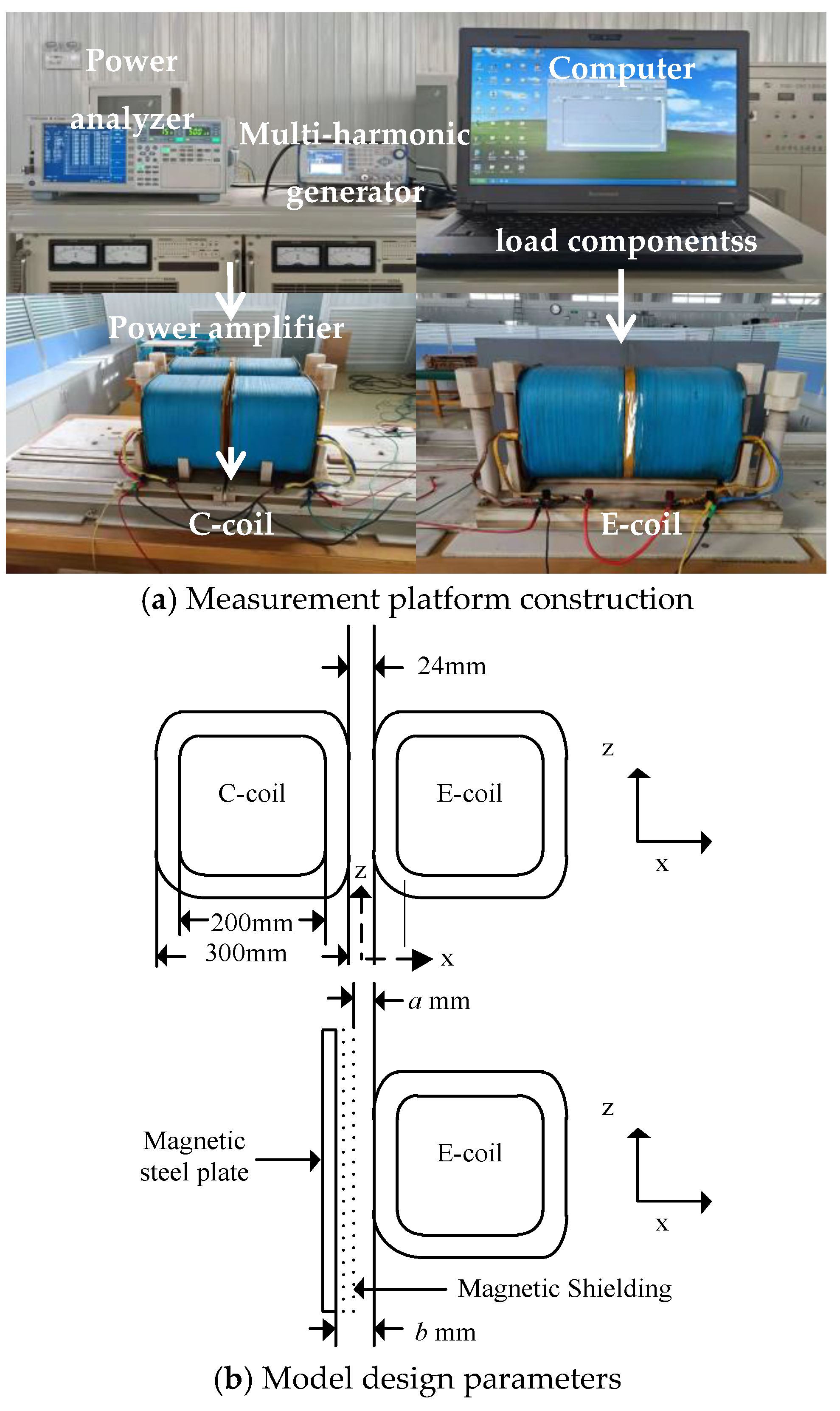
2. Experimental Platform and Strategy for Determination of Stray Loss

The experimental platform was established based on the TEAM P21 model, including the multi-harmonic generator, the high-precision power amplifier, and the power analyzer, as shown in Figure 1a. The schematic diagram of the TEAM P21 model is shown in Figure 1b. All the input data can be found in [31], including the design parameters of models and the electric and magnetic properties of materials.

In the time-varying magnetic field, the metal conductor induces eddy currents and subsequently influences the magnetic field distribution in the conductor. To consider the variation in leakage flux distribution adequately with load components, the paper investigates the stray-field loss with different types of load components and working conditions based on the leakage flux complementary-based measurement method. The basic workflow can be found in [6].

The main difference with respect to previous work is that the distances (D_coil) from the load components to the exciting coils (E-coil) are changed due to the different types of load components, as shown in Figure 1b.

Because the model size is fixed, the variation in leakage flux distribution caused by different D_coil is considered through the following approaches.

(1)

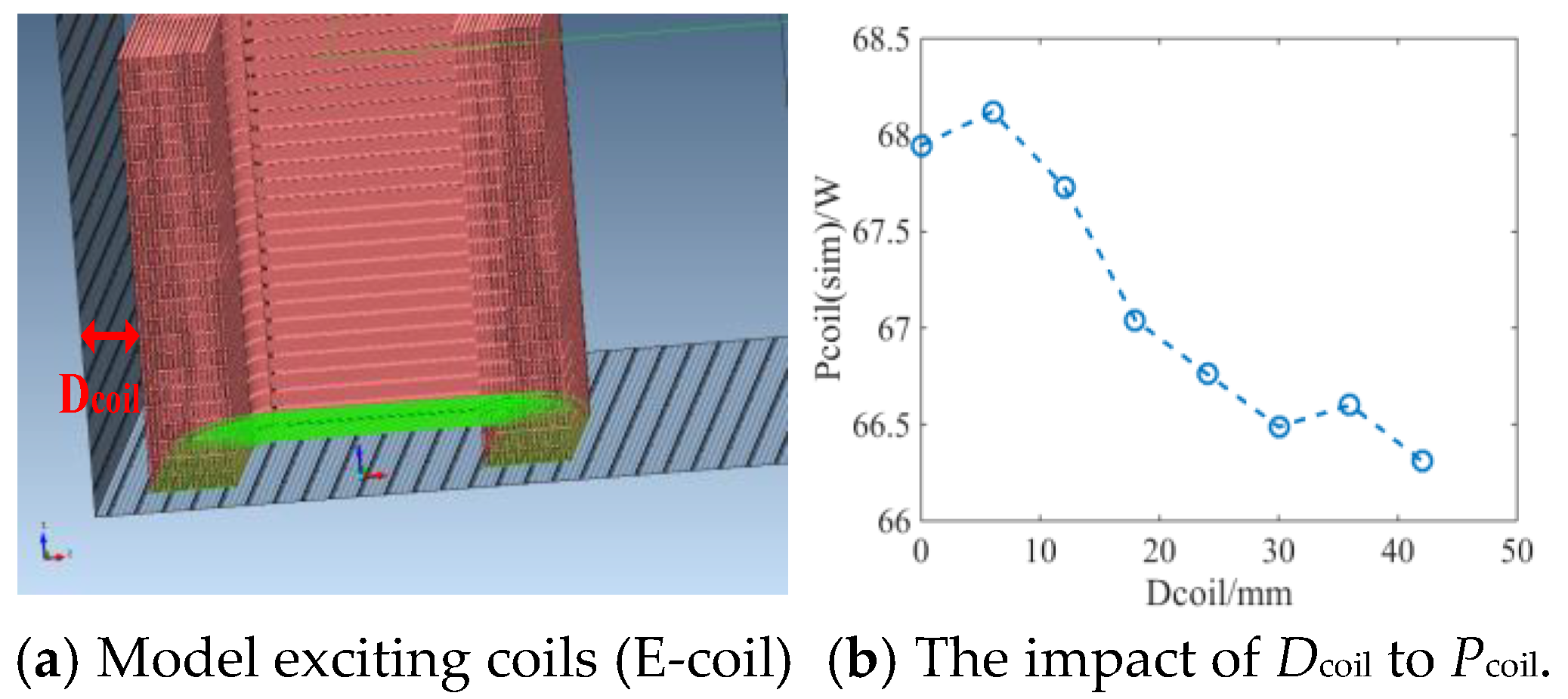
The software Simcenter MAGNET^TM is used to model exciting coils (E-coil) with load components, as shown in Figure 2a, which the version of the software is 7.5. Figure 2b shows that the influence of D_coil on the ohmic loss of the excitation coils (P_coil). Figure 2 shows the simulated ohmic loss of E-coil when the RMS value of the excitation AC current reaches 10 A.

(2)

The distance between the different load components and the windings varies. However, the distance between the compensating coils and the exciting coils is constant (24 mm); a loss coefficient ξ_Dcoil is introduced to take into consideration the loss of the coil varying with D_coil.

$${\xi }_{D_{\mathrm{coil}(xmm)}}={\displaystyle \frac{P_{\mathrm{coil}(xmm)}}{P_{\mathrm{coil}\left(12\mathrm{mm}\right)}}}$$

(2)

$$P_{\mathrm{tm}}=P_{\mathrm{load}}-{\displaystyle \frac{P_{\mathrm{no}-\mathrm{load}(\mathrm{E}+\mathrm{C})}}{2}}\times {\xi }_{D_{\mathrm{coil}\left(\mathrm{xmm}\right)}}$$

(3)

where P_load is the ohmic loss under load condition and P_no-load(E+C) is the ohmic loss measured under no-load condition with C-coils.

All the excitation cases are specified, whatever the load components are (GO, magnetic steel plate, or combined components of both materials), as shown in

Table 1. Excitation conditions.

Cases	Excitation Conditions
I	U1sin(ωt)	In each case, the excitation current (AC) reaches 10 A (rms), but without DC component.
II	U1sin(ωt) + 0.3U1sin(3ωt)
III	U1sin(ωt) + 0.3U1sin(3ωt) + 0.3U1sin(5ωt) + 0.3U1sin(7ωt)
IV	U1sin(ωt) + 0.3U1sin(3ωt) (with DC component)	Hybrid excitation at the same side of model’s part; AC reaches 7 A (rms) and includes DC (5 A).

.

The measured stray-field losses inside the load components are shown in

Table 2. Stray-field loss with different types of load components.

Cases	GO/(W)	Magnetic Steel Plate/(W)	Combined Components/(W)
I	5.77	28.36	5.16
II	6.39	30.51	5.90
III	7.46	32.48	7.03
IV	2.80	15.94	2.92

.

3. Calculation of Loss of GO and Magnetic Steel Plate Under Complex Excitations

This section first derives an analytical formulation of EM parameters of unsaturated hysteresis loop for predicting the hysteresis loss under different flux densities, which can be further employed to calculate the hysteresis loss under NSE. To simplify the calculation of the statistical parameter V₀ under sinusoidal and complex AC-DC hybrid excitations, a simple but effective calculation method is proposed and verified by experimental results. Finally, a method for measuring the magnetic steel plate under NSE is proposed. The effectiveness of the hysteresis loss calculation method is verified by simulations and experiments.

3.1. Energetic Hysteresis Model (EM)

EM is a physical model based on the considerations of energy balance and statistical domain behavior, and calculates the applied field H by magnetization M [27].

$$\begin{array}{l}H=H_{\mathrm{d}}+\mathrm{sgn}(\mathrm{m})H_{\mathrm{r}}+\mathrm{sgn}(\mathrm{m}-{\mathrm{m}}_0)H_{\mathrm{l}}\\ \hspace{1em}=N_{\mathrm{e}}{M}_{\mathrm{s}}\mathrm{m}+\mathrm{sgn}(\mathrm{m})h\left\{{\left[{(1+m)}^{1+m}{(1-m)}^{1-m}\right]}^{g/2}-1\right\}\\ \hspace{1em}+\mathrm{sgn}(\mathrm{m}-{\mathrm{m}}_0)\times ({\displaystyle \frac{k}{{\mu }_0\times M_{\mathrm{s}}}}+c_{\mathrm{r}}{H}_{\mathrm{r}})\times [1-\kappa \exp (-{\displaystyle \frac{\mathrm{q}}{\kappa }}\left|{\mathrm{m}-\mathrm{m}}_0\right|\left)\right]\end{array}$$

(4)

where the demagnetizing field, reversible field, and irreversible field are represented as H_d, H_r, and H_l, respectively. N_e is the demagnetization factor, m = M/M_s is the related magnetization, M is the total magnetization, M_s is the saturated magnetization, h and g relate to the saturated field and anisotropy, k is the hysteresis loss coefficient, q is the adaptive constant related to pinning, and c_r is the ratio of the domain or grain geometry.

Extracting the EM parameters plays a key role in hysteresis loss calculation under both sinusoidal and non-sinusoidal supplies. Traditionally, there are mainly two kinds of methods to solve the saturated hysteresis loop parameters, i.e., using optimization algorithms and solving transcendental equations [21,27]. However, both of these two methods suffer from having a complex numerical calculation procedure and long computation time.

Moreover, using saturated loop parameters to simulate unsaturated hysteresis loops will cause a large error since the hysteresis behavior of magnetic materials is related to the peak value of flux density B [29]. To consider the effect of magnetization contribution on EM parameters, the MEM is proposed to extract the EM parameters of the unsaturated hysteresis loop [29]. However, this method ignores two key issues, i.e., the application range of solving the equation (k = μ₀H_cM_s) and the reproduction of the hysteresis loop, which would result in high errors in the predicted hysteresis loss and loop.

3.2. Improved Energetic Hysteresis Model (IEM)

(1)

Shortcomings in MEM

The basic prerequisite of the selection of EM parameters is that the parameters q and g should meet two prerequisites, i.e., e^−q ≤ 1 and 1 ≤ 2^g [27]. When magnetization M is zero, H_d and H_r equal 0. The loss coefficient k can be calculated by (5).

$$H_{\mathrm{c}}=\left({\displaystyle \frac{k}{{\mu }_0\times M_{\mathrm{s}}}}\right)\times \left[1-\kappa \exp \left(-{\displaystyle \frac{q}{\kappa }}\left|m-m_0\right|\right)\right]$$

(5)

where H_c is the coercivity of the static hysteresis loop, κ is expressed as

$$\kappa =2-{\kappa }_0\exp (-{\displaystyle \frac{q}{{\kappa }_0}}\left|m-m_0\right|)$$

(6)

Because the simulation begins with m₀ = 0 and κ = 1 [27], the values of parameter κ vary from 1 to 2, regardless of how large or small the values of model parameters are. Due to e^−q ≤ 1, A = [1 − κexp(−q/κ|m − m₀|)] is approximately equal to 1 when a strong applied field is applied. Therefore, the equation (k = μ₀H_cM_s) is often used to solve k in the strong applied field, but not in the weak applied field. Nevertheless, in MEM, this equation is still used to solve the k in the weak applied field.

To point out the defects of MEM, two materials (Q235A and B27R090) are selected for checking the performance of the MEM, where the saturated hysteresis loop parameters were shown in

Table 3. EM parameters of the saturated loop.

	Ms (×106 A/m)	Ne (×10−5)	h (A/m)	g	q	cr
Q235A	1.55	14.71	56.80	10.06	32.57	0.27
B27R090	1.55	1.03	0.14	12.82	35.95	0.92

using the optimization algorithm. The comparison of simulated saturated static hysteresis loops with measured saturated static hysteresis loops is shown in Figure 3.

Based on the energetic model parameters corresponding to the saturated static hysteresis loop shown in Table 3, we analyzed the limitations of the MEM model in predicting the static hysteresis loop of materials under unsaturated magnetization conditions, as illustrated in Figure 4. The reason for large loss prediction errors is that the equation (k = H_c × μ₀ × M_s) is not always true in the weak applied field, which would result in a high error.

(2)

Improved Energetic hysteresis model (IEM)

Firstly, the law of influence of EM parameters on hysteresis characteristics is investigated using the method of control variate.

Table 4. The influence of EM parameters on hysteresis characteristics.

	Ne ↑	h ↑	g ↑	q ↑	cr ↑	k ↑
Br	↓	↓	↓	↑	↑	↑
Hc	---	---	---	↑	---	↑
Hmax	↑	↑	↑	↑	↑	↑
Loop area	---	↑	↑	↑	↑	↑

shows the influence of each EM parameter on the hysteresis loop; the horizontal segment (---) in Table 4 means that the characteristic quantity is not affected by the characteristic parameters, so that can be ignored. The arrow (↑) means that characteristic quantity (Br, Hc, Hmax, Loop area) increase with the increase of EM parameters.The arrow (↓) means that characteristic quantity (Br, Hc, Hmax, Loop area) decrease with the increase of EM parameters.

Secondly, only hysteresis loss coefficient k determines the value of coercivity (H_c) according to EM equations. To consider the influence of peak induction flux densities B on H_c, this paper proposes an improved calculation method to extract the parameter k_B at various peak induction flux densities B by the following equation, where B_s is the saturation flux density.

$$k_B={\displaystyle \frac{H_C\times {\mu }_0\times M_s}{[1-\exp (-q\left|\frac{B}{B_S}\right|)]}}$$

(7)

By comparing simulated results using Equation (7) with those by experiments and the MEM, Equation (7) has better capability in predicting hysteresis loss compared to MEM from Figure 3.

A hysteresis loss error metric δ₁ is defined to check the hysteresis loss prediction accuracy and is expressed as

$${\delta }_1=\left|\left(P_{\mathrm{cal}}-P_{\mathrm{mea}}\right)/P_{\mathrm{mea}}\right|\times 100\%$$

(8)

where the P_cal is the simulated hysteresis loss and P_mea is the measured hysteresis loss.

The measured results of hysteresis loss W_hys(mea) and error metric δ₁ are given in

Table 5. Calculated and measured results under different flux densities.

B (T)	B27R090
	Whys(mea)	δ1(IEM) (%)	δ1(MEM) (%)
0.11 T	17.12	5.08	−85.11
0.18 T	44.40	−0.38	−41.61
0.23 T	65.43	−0.62	−29.18
0.28 T	94.14	−0.96	−19.73
0.34 T	124.20	4.14	−8.24
0.38 T	155.19	0.11	−8.41
0.42 T	189.50	0.13	−5.61

(B27R090).

The error metric δ₁ of simulated hysteresis loss using Equation (7) is less than 10%, implying that these parameters (h, g, q, and c_r) of the reversible field and irreversible field component are only barely affected by the peak value of flux density.

The parameters that determine the reversible field characterization of the EM are the material anisotropy coefficient g and the saturation field scaling factor h. The anisotropy coefficient g is related to the orientational arrangement of atoms within the crystal. The saturation field scaling factor h is related to the ratio of the magnetization strength M to the magnetic field strength H, so we assume that h varies with the magnetization.

An analytical formulation is proposed to extract the saturated magnetic field proportion coefficient h at various peak induction flux densities B by the maximum of measured magnetic field strength (H_max-mea), where N_e(Bs), M_s, q, c_r, and g are saturated parameters of EM, shown in Table 3.

$$h_{(B)}={\displaystyle \frac{h_{(B_s)}(H_{\max -\mathrm{mea}(B)}–N_e{M}_s\frac{B}{B_S}-\frac{k_B}{{\mu }_0{M}_s}(1-\exp (-q\left|\frac{B}{B_S}\right|)))}{(1+c_r(1-\exp (-q\left|\frac{B}{B_S}\right|)))H_{r(Bs)}}}$$

(9)

where

$$H_{r(B)}=h\left\{\left.{[{(1+{\displaystyle \frac{B}{B_S}})}^{1+{\displaystyle \frac{B}{B_S}}}{(1-{\displaystyle \frac{B}{B_S}})}^{1-{\displaystyle \frac{B}{B_S}}}]}^{g/2}-1\right\}\right.$$

(10)

By comparing simulated results calculated by IEM with those by experiments and MEM, the accuracy of IEM is significantly improved without sacrificing its simplicity, as shown in Figure 5.

3.3. Calculation and Verification of Magnetic Loss of GO Under Harmonic Excitations

For hysteresis loss calculation under non-sinusoidal supplies, the relationship between hysteresis loss and the hysteresis magnetic field H_hys can be expressed as

$$W_{\mathrm{hys}}={\displaystyle \underset{l}{\oint }{H}_{\mathrm{hys}}\mathrm{d}B}$$

(11)

The non-sinusoidal flux density waveforms were inputted into (4); the corresponding hysteresis loss was obtained by (11), since the EM parameters were independent of frequency and flux density waveform [27].

Because the GO are thin enough, the eddy current skin phenomenon is less visible under low frequency. The eddy current loss W_eddy can be calculated according to the following formulation [19].

$$W_{\mathrm{eddy}}={\displaystyle \frac{\sigma d^2}{12}}{{\displaystyle {\int }_0^T(\frac{\mathrm{d}B(t)}{\mathrm{d}t})}}^2\mathrm{d}t$$

(12)

where d is the thickness and σ is the conductivity.

Based on the Statistical Theory of Losses [19], the excess loss W_exc can be calculated by

$$W_{\mathrm{exc}}=\sqrt{\sigma SG{V}_0}{{\displaystyle {\int }_0^T\left|\frac{\mathrm{d}B(t)}{\mathrm{d}t}\right|}}^{1.5}\mathrm{d}t=W-W_{\mathrm{hys}}-W_{\mathrm{eddy}}$$

(13)

where V₀ is the statistical parameter, S is the cross-sectional area, and G = 0.1356 is the dimensionless coefficient. Many studies reported that the types of excitations without DC component and eddy current skin phenomenon have little influence on the statistical parameter V₀ [19,21]. The value of statistical parameter V₀ in the power frequency range can be used to calculate the excess loss under harmonic excitations, where the fundamental frequency of NSE is 50 Hz.

Figure 6 shows the relative error δ of predicted magnetic loss under harmonic excitations, where the harmonic excitations cases are specified as shown in

Table 6. Excitation conditions of GO under harmonic excitations.

Cases	Excitation Conditions
HE I	U1 sin (ωt) + 0.9U1 sin (3ωt + θ)	θ = 0°, 45°, 90°, 135°, 180°
HE II	U1 sin (ωt) + 1.5U1 sin (5ωt + θ)	θ = 0°, 45°, 90°, 135°, 180°

; δ is expressed as

$$\delta =({\displaystyle \frac{P_{\mathrm{sim}}}{P_{\mathrm{mea}}}}-1)\times 100\%$$

(14)

3.4. Calculation and Verification of Magnetic Loss of GO Under Harmonic and DC Hybrid Excitations

The hysteresis loss and eddy current loss are still calculated in the same way as in Section 3.3. Notably, the excess loss originates from the movement of the domain walls and additional heat produced by eddy currents, implying that the DC bias component affects statistical parameter V₀ [32].

The static hysteresis loss is associated with the irreversible magnetization process. As the amplitude of the flux density increases, the rotation of the magnetic domains intensifies; the static hysteresis loss also rises. Biased magnetization elevates the actual magnetic flux density, further contributing to an increase in static hysteresis loss. Eddy current losses are related to the rate of change in magnetic flux density and are not influenced by DC bias. Excess losses arise from both the static hysteresis loss and the thermal effects of eddy currents. The presence of DC bias leads to an increase in static hysteresis loss, which subsequently contributes to an increase in excess loss as well. Currently, there is a lack of comprehensive theoretical studies examining the influence of DC bias on static hysteresis loss and excess loss. Therefore, extensive measurements are necessary to accurately predict the effects of DC bias on magnetic losses. It is impossible to predict the influence of DC bias on the loss without performing extensive measurements. To simplify the computational workflow, a loss-map, which expresses the magnetic loss under DC bias, is established, as shown in Figure 7. It was hypothesized that the magnitude of statistical parameter V₀ is determined by peak AC induction B_ac and DC bias magnetic field H_b. The statistical parameter V₀ can be calculated from the loss-map.

Figure 8 shows the relative error δ of predicted magnetic loss under harmonic and DC hybrid excitations, where the excitations cases are specified as shown in

Table 7. Excitation conditions of GO under harmonic and DC hybrid excitations.

Cases	Excitation Conditions
H + DC E I	U1 sin (ωt) + 0.9U1 sin (3ωt + θ) + Idc	θ = 0°, 90°, 180°. Hdc = 20, 40, 60 A/m
H + DC E II	U1 sin (ωt) + 1.5U1 sin (5ωt + θ) + Idc	θ = 0°, 90°, 180° Hdc = 20, 40, 60 A/m

.

3.5. Calculation Method of Hysteresis Loss of Magnetic Steel Plate Under Complex Excitation Conditions

Figure 9 shows the experimental platform for measuring magnetic properties of the magnetic steel plate of the ring specimen.

Table 8. Parameters of ring specimen.

Turns of Ring Specimen	Outer Diameter (mm)	Inner Diameter (mm)	Height (mm)	Conductivity (S/m)
1800	95	100	9.5	6484,000

shows the design parameters of the ring specimen.

Note that the calculation method of classical eddy current loss is not capable of predicting ohmic loss due to edge effects, because the length and width of the ring specimen are not much larger than the height.

Therefore, to reduce the difference between the magnetic properties represented by average magnetic flux density and the real properties of the material, the data of magnetic properties at low-frequency (3 Hz) is measured, where the skin depth of the magnetic steel plate of the ring specimen ξ = 4 mm is significantly larger than the thickness (2.5 mm) of the steel ring, implying that the eddy current skin phenomenon can generally be neglected.

When ignoring the eddy current skin phenomenon, whatever the magnetization law B(H) is, the eddy current loss generated in the magnetic material is the same as long as the waveform of magnetic flux density is the same [33]. To ensure that the simulation flux density waveform is consistent with the actual magnetic flux density waveform, the current waveform is obtained by linear interpolation, as shown in Figure 10.

Secondly, the eddy current loss of the ring specimen under harmonic excitation is calculated by finite element method (FEM), where the current source is used to generate a magnetic field.

Finally, the hysteresis loss under complex excitation conditions is determined indirectly by subtracting the eddy current loss calculated by FEM from the total measured magnetic loss.

When frequency f = 3 Hz, the skin depth of the magnetic steel plate of the ring specimen ξ = 4 mm is significantly larger than the thickness (2.5 mm) of the steel ring so that the results of hysteresis loss under complex excitation determined by the indirect method are justified.

The FEM model is shown in Figure 11a. The comparison between the simulated and the measured flux density waveform is shown in Figure 11b.

Figure 12 shows the relative error δ of predicted hysteresis loss using IEM under harmonic excitations, where the IEM parameters are shown in Table 3 and the harmonic excitations cases are specified as shown in

Table 9. Excitation conditions of magnetic steel plate under harmonic and DC hybrid excitations.

Cases	Excitation Conditions
H E	U1 sin (ωt) + 1.5U1 sin (5ωt + θ)	θ = 0°, 90°, 180°

.

4. Modeling Method for Stray-Field Loss

This section first discusses the advantages and limitations of existing numerical approaches of additional loss. Then, an effective computational strategy for stray-field loss with different types of load components is established.

4.1. Analysis of Existing Methods of Additional Loss

The results of eddy current loss of load components obtained by FEM are accurate enough through refined finite element modeling (3-D eddy current region), where the conductivity of GO is shown in (15).

$$[\sigma ]=\left[\begin{array}{l}\begin{array}{ccc}{\sigma }_x& & \end{array}\\ \begin{array}{ccc}& {\sigma }_y& \end{array}\\ \begin{array}{ccc}& & {\sigma }_z\end{array}\end{array}\right]$$

(15)

The reasonably simplified finite element modeling can not only reduce the computational cost but also separate the eddy current loss under a specific condition, approximately. The additional loss is generated by the leakage magnetic flux perpendicular to the load components and is part of total eddy current loss. The first modeling approach is that the conductivity of GO, which is perpendicular to the lamination, is forced to zero to include the eddy current loss caused by the leakage magnetic flux perpendicular to the load components only (2-D eddy current region), as shown in (16).

$$[\sigma ]=\left[\begin{array}{l}\begin{array}{ccc}0& & \end{array}\\ \begin{array}{ccc}& {\sigma }_y& \end{array}\\ \begin{array}{ccc}& & {\sigma }_z\end{array}\end{array}\right]$$

(16)

Note that the eddy current loss (P_eddy-main) generated by the main magnetic flux inside the magnetic materials is completely ignored, whereupon P_eddy-main needs to be calculated by the magnetic loss model. However, the drawback with this method is that it is only applicable to the case in which the eddy current skin phenomenon can be completely ignored.

The second modeling approach is that the eddy current region is divided into two parts, i.e., 2-D eddy current region and 3-D eddy current region. Note that the eddy current loss calculated from the 3-D eddy current region includes the P_a and P_eddy-main, whereupon the eddy current loss needs to be removed from the magnetic loss model to avoid overestimates of specific total magnetic loss.

4.2. Computational Strategy of Stray-Field Loss with Different Types of Load Components

The thickness of the shielded magnetic steel plate can reach 10 mm. When there is no magnetic shielding, the skin phenomenon will be very obvious under the power frequency condition. Therefore, the demagnetization effect of the eddy current cannot be ignored; that is, the accurate separation of additional loss cannot be realized.

For the different types of load components, the part of GO closest to the excitation coil and farthest from the excitation coils, and the magnetic steel plate are modeled individually and treated as the 3-D eddy current regions. The remaining GO are modeled as bulk material, regarded as the 2-D eddy current region.

For the part of solving 3-D eddy current regions, the hysteresis and excess loss generated by the main magnetic flux inside the magnetic material is superimposed with the eddy current loss calculated from 3-D eddy current regions by FEM. For the part of solving 2-D eddy current regions, the loss generated by the main magnetic flux inside the magnetic material is superimposed with the eddy current loss calculated from 2-D eddy current regions by FEM.

In this paper, the magnetic field data are extracted. Based on the magnetic loss calculation method under complex excitation in Section 3, the specific total magnetic loss is calculated and superimposed with the eddy current loss to obtain the stray-field loss of the load components. The stray-field loss can be calculated by

$$\begin{array}{l}{P}_{\mathrm{tm}}=P_{\mathrm{hys}}+P_{\mathrm{exc}}+P_{\mathrm{eddy}}\\ \hspace{1em}={\displaystyle \sum _{e=1}^{N{\mathrm{um}}_e}(P_{\mathrm{hys}}^e(B{(t)}^e+P_{\mathrm{exc}}^e(B{(t)}^e)}\rho V^e+P_{\mathrm{eddy}}\end{array}$$

(17)

where V^e is the volume per element, Num_e is the total number of elements in the laminated sheets, and ρ is the body density.

5. Calculation and Verification

To verify the effectiveness of the numerical calculation method, the simulated stray-field loss with different types of load components is compared with the experimental results, as shown in

Table 10. Simulation and Measurement of Stray-field loss with different types of load components.

Cases	GO/(W)		Magnetic Steel Plate/(W)		Combined Components/(W)
	Mea	Cal	Mea	Cal	Mea	Cal
I	5.77	5.54	28.36	27.69	5.16	5.37
II	6.39	6.11	30.51	30.03	5.90	5.73
III	7.46	6.91	32.48	32.43	7.03	6.79
IV	2.80	2.60	15.94	15.04	2.92	2.67

.

Moreover, for validation of the numerical simulation results, the comparison between the simulated and the measured leakage magnetic field is shown in Figure 13, where the 1/2 thickness d of the probe of Gauss/Teslameter (Model 7010) is 0.76 mm. The measured and calculated results are in good agreement, where x = 3 + d.

6. Conclusions

The calculation of stray-field loss for typical magnetic load components under NSE is investigated theoretically and practically. Important conclusions are described below.

(1)

The distribution of the leakage flux around the coil depends not only on the types of load components, but also on the distance D_coil between the load components and the coil. The improved method proposed can not only consider the distribution of the leakage flux around the coil, but also consider the influence of the D_coil on the coil loss, so as to more accurately separate the stray-field loss of load components from the total loss.

(2)

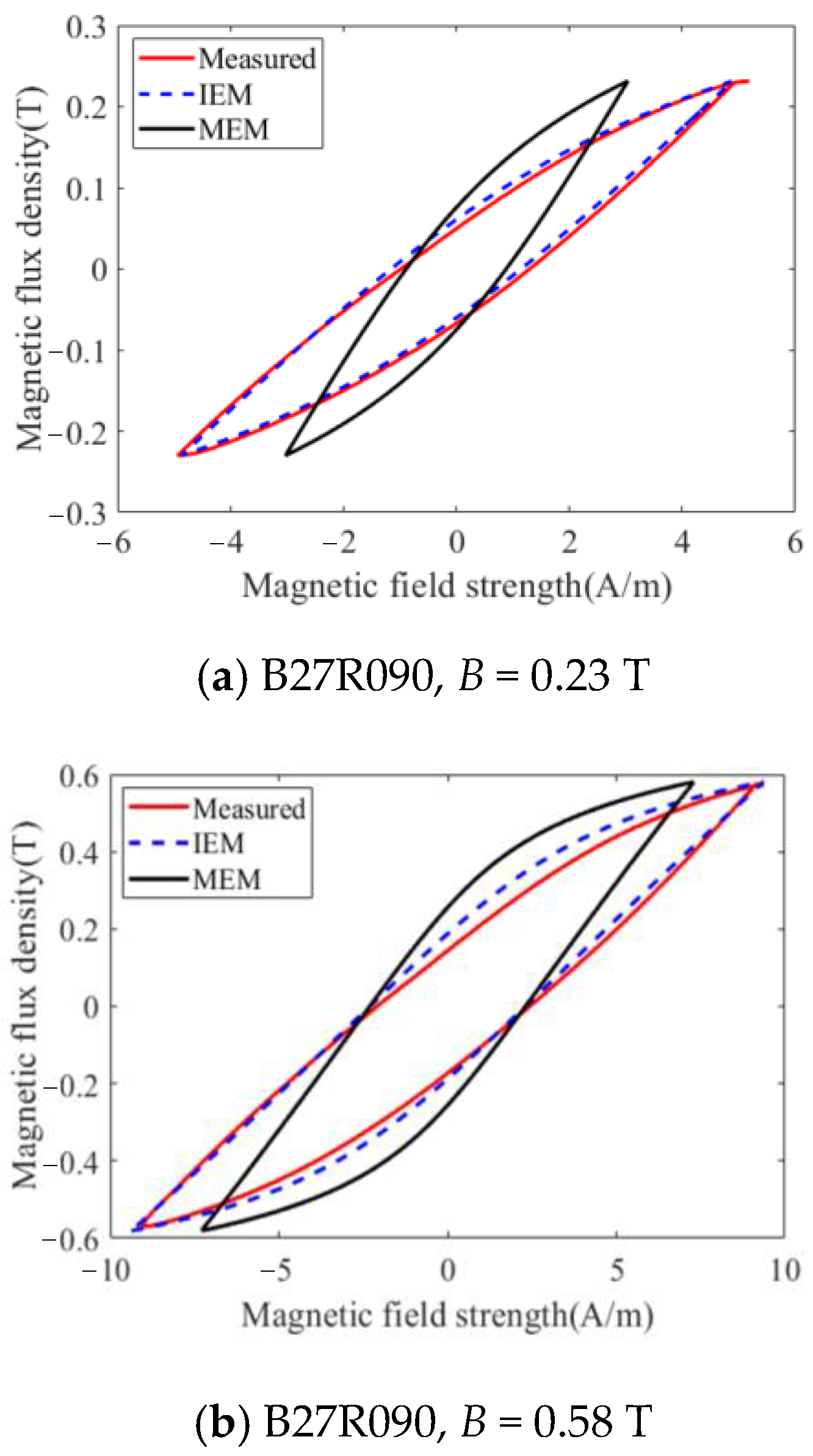
By considering the scope of application of equation (k = μ₀H_CM_s) and the effect of magnetization contribution on EM parameters, the IEM is proposed which can not only reduce the dependence on measurement data for calculating model parameters but also successfully improves the accuracy of hysteresis loss and loop compared to the MEM, where the hysteresis loss coefficient k and saturated magnetic field proportion coefficient h are derived theoretically and validated by experiments.

(3)

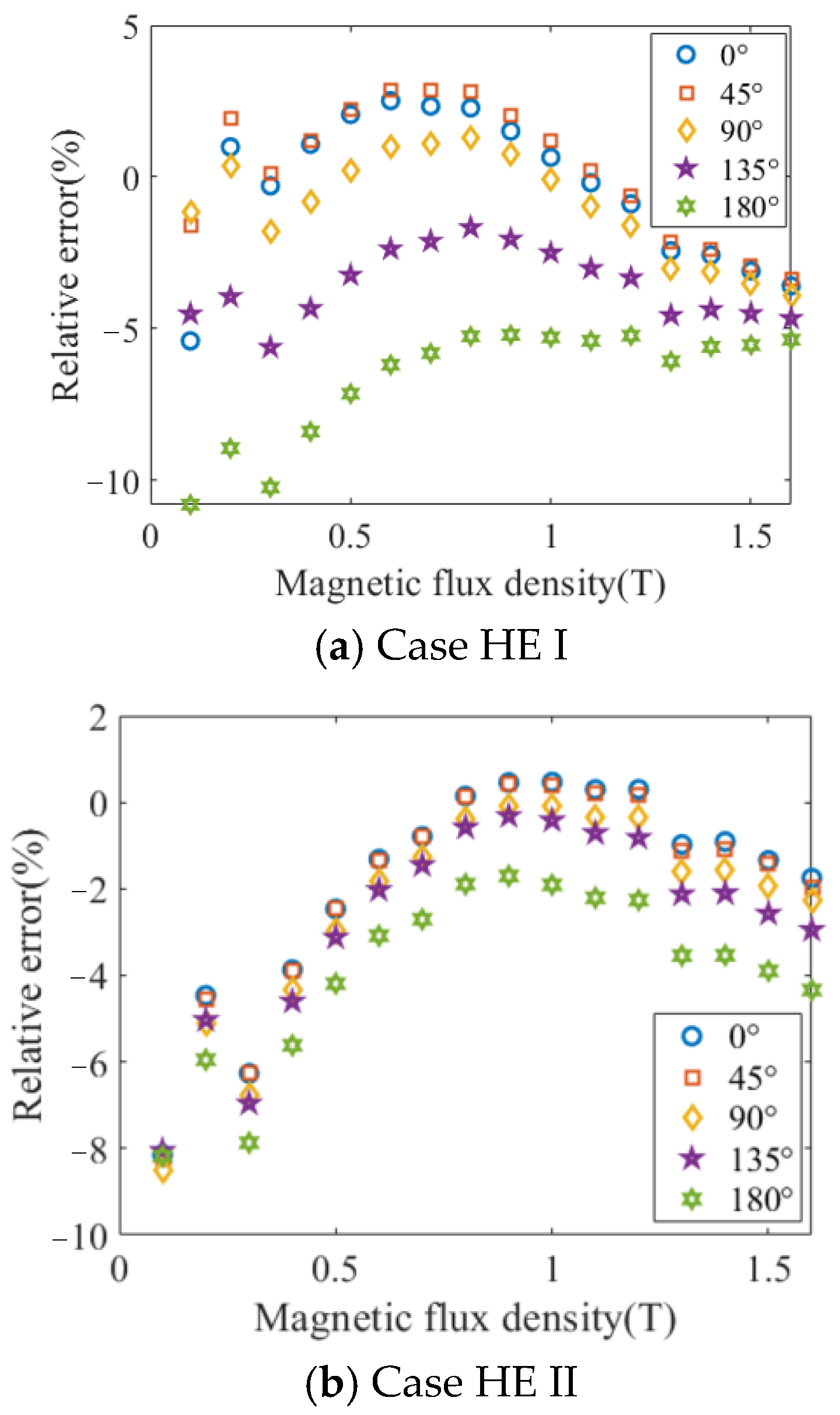
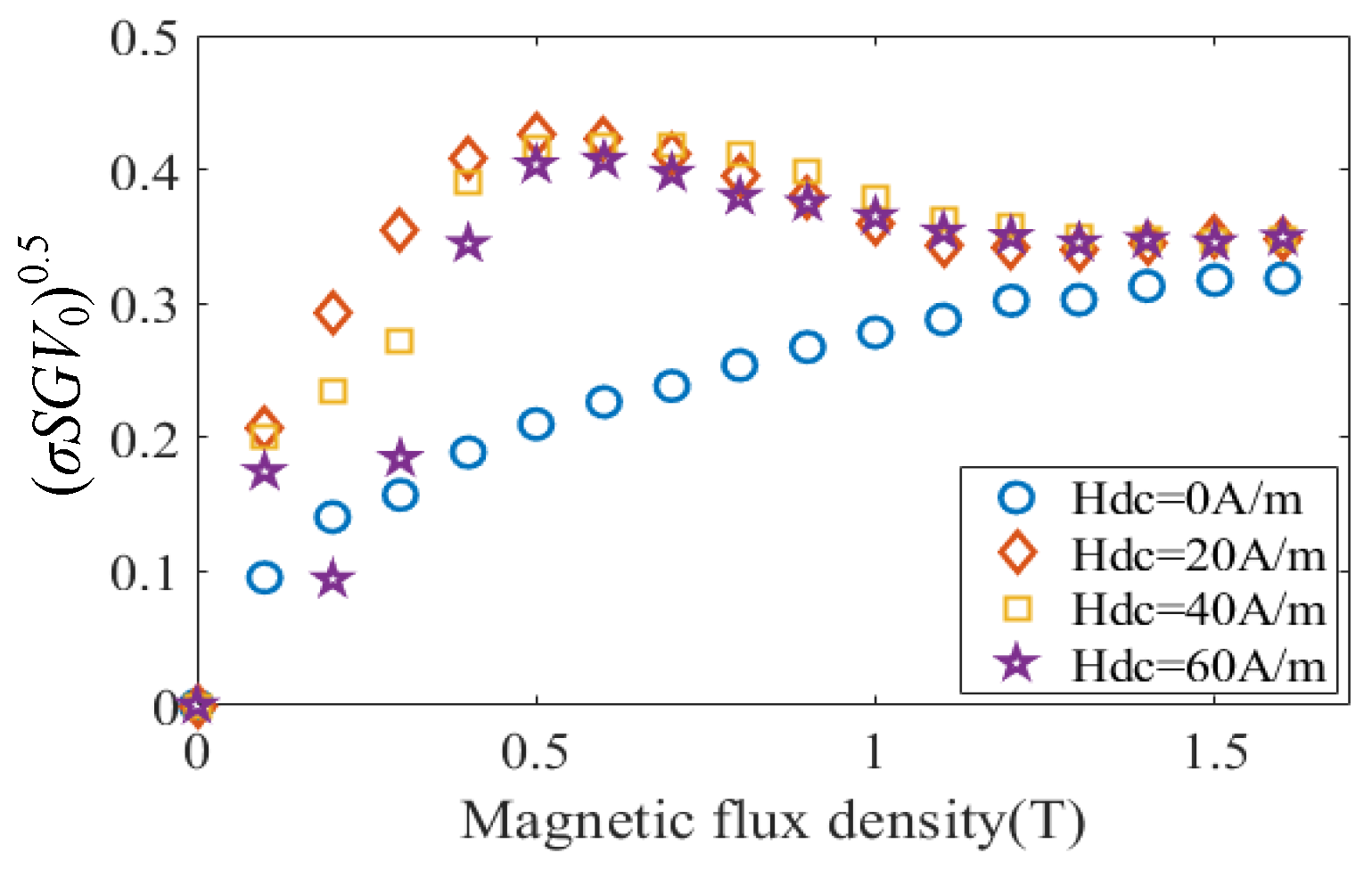
To predict the influence of DC magnetization on the loss, the loss-map, which expresses the magnetic loss under DC bias, is established. Based on the STL, the loss calculation method under sinusoidal, harmonic, and harmonic and DC hybrid excitations is proposed and validated by experiments.

(4)

By discussing the advantages and limitations of existing numerical approaches of additional loss, it could be found that the 2-D eddy current region is only applicable to the case in which the eddy current skin phenomenon can be completely ignored. Considering the influence of the eddy current field modeling method on the stray-field loss computational strategy, the stray-field loss calculation method of GO, magnetic steel plate, and combined components of both materials under complex excitations is established. The effectiveness of the stray loss calculation method is verified by comparing the stray-field loss and leakage magnetic field experimental results with the simulation results.

(5)

The proposed method can be used to calculate transformer stray losses, offering theoretical support for transformer design. This approach addresses both the reliability and high efficiency needs of transformers, providing a theoretical foundation for modeling the electromagnetic thermal optimization constraints of transformers.

References

1. Schäfer, J.; Rohner, G.; Kolar, J.W. Extending the Steinmetz Equation: Incorporating Mechanical Stress Effects in Ferrite Core Loss Calculations. IEEE Open J. Power Electron. 2025, 6, 56–65. [Google Scholar] [CrossRef]
2. Gömöry, F.; Šouc, J.; Solovyov, M.; Ries, R.; Hintze, C.; Landvogt, S.; Pekarčíková, M.; Christensen, J.J.; Bahl, C.R.; Jørgensen, N.O.; et al. Hysteresis and Coupling Loss in Filamentized REBCO Tapes. IEEE Trans. Appl. Supercond. 2025, 35, 5900205. [Google Scholar] [CrossRef]
3. Kwon, J.; Sa, J.; Lee, S.; Jang, G. A Voltage Minimization Control Method for Magnetic Navigation Systems to Enhance the Rotating Magnetic Field. IEEE Robot. Autom. Lett. 2024, 9, 11561–11568. [Google Scholar] [CrossRef]
4. Sato, H.; Kotani, J.; Sasaki, Y.; Tomioka, S.; Takizawa, T.; Ueda, Y.; Kimiya, H.; Igarashi, H. Analysis of Magnetic Properties of Soft Magnetic Composite Using Magnetic Circuits Generated by Discrete Element Method. IEEE Trans. Magn. 2024, 60, 7402807. [Google Scholar] [CrossRef]
5. Li, C.; Cheng, M.; Qin, W.; Wang, Z.; Ma, X.; Wang, W. Analytical Loss Model for Magnetic Cores Based on Vector Magnetic Circuit Theory. IEEE Open J. Power Electron. 2024, 5, 1659–1670. [Google Scholar] [CrossRef]
6. Hossain, M.S.; Islam, M.R.; Sutanto, D.; Muttaqi, K.M. Advanced Soft Magnetic Materials for the Development of High-Frequency Magnetic Core Used in Solid-State Transformers. IEEE Trans. Appl. Supercond. 2024, 34, 5501105. [Google Scholar] [CrossRef]
7. Li, Y.; Li, Y.; Lin, Z.; Yue, S.; Chen, R.; Guo, P.; Liu, J. A Hysteresis Model for Soft Magnetic Composites Considering Particle Size Distribution. IEEE Trans. Magn. 2024, 60, 7301405. [Google Scholar] [CrossRef]
8. Kanakgiri, K.; Bhardwaj, D.I.; Ram, B.S.; Kulkarni, S.V. A Circuit-Based Formulation for Soft Magnetic Materials Using the Jiles–Atherton Model. IEEE Trans. Magn. 2024, 60, 7301107. [Google Scholar] [CrossRef]
9. Zhao, X.; Cao, Y.; Cheng, Z.; Forghani, B.; Liu, L.; Wang, J. Experimental and numerical study on stray loss in laminated magnetic shielding under 3-D AC-DC hybrid excitations for HVDC transformers. IEEE Access 2020, 8, 144432–144441. [Google Scholar] [CrossRef]
10. Wang, J.; Dagan, K.J.; Yuan, X.; Wang, W.; Mellor, P.H. A practical approach for core loss estimation of a high-current gapped inductor in PWM converters with a user-friendly loss map. IEEE Trans. Power Electron. 2019, 34, 5697–5710. [Google Scholar] [CrossRef]
11. Steinmetz, C.P. On the law of hysteresis. Proc. IEEE 1984, 72, 197–221. [Google Scholar] [CrossRef]
12. Reinert, J.; Brockmeyer, A.; De Doncker, R.W.A.A. Calculation of losses in ferro- and ferrimagnetic materials based on the modified Steinmetz equation. IEEE Trans. Ind. Appl. 2001, 37, 1055–1061. [Google Scholar] [CrossRef]
13. Li, J.; Abdallah, T.; Sullivan, C.R. Improved calculation of core loss with nonsinusoidal waveforms. In Proceedings of the Conference Record of the 2001 IEEE Industry Applications Conference. 36th IAS Annual Meeting (Cat. No.01CH37248), Chicago, IL, USA, 30 September–4 October 2001; pp. 2203–2210. [Google Scholar]
14. Mulethaler, J.; Biela, J.; Kolar, J.W.; Ecklebe, A. Improved core loss calculation for magnetic components employed in power electronic systems. IEEE Trans. Power Electron. 2012, 27, 964–973. [Google Scholar] [CrossRef]
15. Shen, W.; Wang, F.; Boroyevic, D.; Tipton, C.W. Loss characterization and calculation of nanocrystalline cores for high-frequency applications. IEEE Trans. Power Electron. 2008, 23, 475–484. [Google Scholar] [CrossRef]
16. Barg, S.; Ammous, K.; Mejbri, H.; Ammous, A. An improved empirical formulation for magnetic core losses estimation under nonsinusoidal induction. IEEE Trans. Power Electron. 2017, 32, 2146–2154. [Google Scholar] [CrossRef]
17. Novak, G.; Kokošar, J.; Nagode, A.; Petrovič, D.S. Core-loss prediction for non-oriented electrical steels based on the steinmetz equation using fixed coefficients with a wide frequency range of validity. IEEE Trans. Magn. 2015, 51, 2001507. [Google Scholar] [CrossRef]
18. Bertotti, G.; Fiorillo, F.; Soardo, G.P. The prediction of power losses in soft magnetic materials. Le J. Phys. Colloq. 1988, 49, 1915–1919. [Google Scholar] [CrossRef]
19. Fiorillo, F.; Novikov, A. An improved approach to power losses in magnetic laminations under nonsinusoidal induction waveform. IEEE Trans. Magn. 1990, 26, 2904–2910. [Google Scholar] [CrossRef]
20. Eggers, D.; Steentjes, S.; Hameyer, K. Advanced iron-loss estimation for nonlinear material behavior. IEEE Trans. Magn. 2012, 48, 3021–3024. [Google Scholar] [CrossRef]
21. Liu, R.; Li, L. Analytical prediction model of energy losses in soft magnetic materials over broadband frequency range. IEEE Trans. Power Electron. 2021, 36, 2009–2017. [Google Scholar] [CrossRef]
22. Zhao, H.; Ragusa, C.; Appino, C.; Barrière, O.; Wang, Y.; Fiorillo, F. Energy losses in soft magnetic materials under symmetric and asymmetric induction waveforms. IEEE Trans. Power Electron. 2019, 34, 2655–2665. [Google Scholar] [CrossRef]
23. Zhao, Z.; Hu, X. Modified loss separation in FeSi laminations under arbitrary distorted flux. AIP Adv. 2020, 10, 085222. [Google Scholar] [CrossRef]
24. Lavers, J.; Biringer, P.; Hollitscher, H. A simple method of estimating the minor loop hysteresis loss in thin laminations. IEEE Trans. Magn. 1978, 14, 386–388. [Google Scholar] [CrossRef]
25. Jiles, D.C.; Thoelke, J.B.; Devine, M.K. Numerical determination of hysteresis parameters for the modeling of magnetic properties using the theory of ferromagnetic hysteresis. IEEE Trans. Magn. 1992, 28, 27–35. [Google Scholar] [CrossRef]
26. Dlala, E. Efficient algorithms for the inclusion of the preisach hysteresis model in nonlinear finite-element methods. IEEE Trans. Magn. 2011, 47, 395–408. [Google Scholar] [CrossRef]
27. Hauser, H. Energetic model of ferromagnetic hysteresis: Isotropic magnetization. J. Appl. Phys. 2004, 96, 2753–2767. [Google Scholar] [CrossRef]
28. Li, Y.; Zhu, J.; Zhu, L.; Li, Y.; Lei, G. A dynamic magnetostriction model of grain-oriented sheet steels based on Becker–Döring crystal magnetization model and Jiles-Atherton theory of magnetic hysteresis. IEEE Trans. Magn. 2020, 56, 7511405. [Google Scholar] [CrossRef]
29. Liu, R.; Li, L. Accurate symmetrical minor loops calculation with a modified energetic hysteresis model. IEEE Trans. Magn. 2020, 56, 7510204. [Google Scholar] [CrossRef]
30. Takahashi, N.; Sakura, T.; Cheng, Z. Nonlinear analysis of eddy current and hysteresis losses of 3-D stray field loss model (Problem 21). IEEE Trans. Magn. 2001, 37, 3672–3675. [Google Scholar] [CrossRef]
31. Cheng, Z.; Forghani, B.; Du, Z.; Liu, L.; Li, Y.; Zhao, X.; Liu, T.; Cai, L.; Zhang, W.; Lu, M.; et al. Modeling and validation of stray-field loss inside magnetic and non-magnetic components under harmonics-DC hybrid excitations based on updated TEAM Problem 21. COMPEL 2021, 40, 941–960. [Google Scholar] [CrossRef]
32. Zirka, S.E.; Moroz, Y.I.; Steentjes, S.; Hameyer, K.; Chwastek, K.; Zurek, S.; Harrison, R. Dynamic magnetization models for soft ferromagnetic materials with coarse and fine domain structures. J. Magn. Magn. Mater. 2015, 394, 229–236. [Google Scholar] [CrossRef]
33. Bertotti, G. Hysteresis in Magnetism for Physicists, Materials Scientists, and Engineers; Academic Press: San Diego, CA, USA; London, UK; Boston, MA, USA; New York, NY, USA; Sydney, Australia; Tokyo, Japan; Toronto, ON, Canada, 1998. [Google Scholar]
Figure 1. Design parameters of TEAM Problem 21 benchmark models.
Symmetry 17 00189 g001
Figure 2. The simulated ohmic loss of E-coil when the RMS value of the excitation AC current reaches 10 A.
Symmetry 17 00189 g002
Figure 3. Prediction of static hysteresis properties of materials under saturated magnetization conditions, where the material tested of (a) is Q235A, the material tested of (b) is B27R090.
Symmetry 17 00189 g003aSymmetry 17 00189 g003b
Figure 4. Comparison between the simulated and the measured hysteresis loops, where the material tested of (a) is Q235A, the material tested of (b) is B27R090.
Symmetry 17 00189 g004
Figure 5. Comparison between the simulated and measured hysteresis loops.
Symmetry 17 00189 g005
Figure 6. Results of relative error of magnetic loss under harmonic excitations.
Symmetry 17 00189 g006
Figure 7. Relationship between the B and (σSGV0)0.5.
Symmetry 17 00189 g007
Figure 8. Results of relative error of magnetic loss under harmonic and DC hybrid excitations.
Symmetry 17 00189 g008
Figure 9. Experimental platform of ring specimen.
Symmetry 17 00189 g009
Figure 10. Calculation of the exciting current.
Symmetry 17 00189 g010
Figure 11. Simulation model and calculation results.
Symmetry 17 00189 g011
Figure 12. Results of relative error of hysteresis loss under complex excitations.
Symmetry 17 00189 g012
Figure 13. Comparison between the simulated and measured leakage field (Case III).
Symmetry 17 00189 g013