Article

Research on a Class of Optimization Problems of Higher Education Cost with Cobb–Douglas Constraint Condition

1
Institute of Higher Education, Shanghai University, Shanghai 200444, China
2
Faculty of Education, East China Normal University, Shanghai 200062, China
3
Xianda College of Economics & Humanities, Shanghai International Studies University, Shanghai 200083, China
*
Authors to whom correspondence should be addressed.
Symmetry 2025, 17(12), 2035; https://doi.org/10.3390/sym17122035
Submission received: 29 October 2025 / Revised: 17 November 2025 / Accepted: 20 November 2025 / Published: 28 November 2025
(This article belongs to the Special Issue Symmetry in Data Analysis and Optimization)

Abstract

This study focuses on a class of optimization problems about higher education costs with industrial production characteristics, in which the objective function is a quadratic cost function and the nonlinear constraints follow the Cobb–Douglas form. Through variable substitution, this class of nonlinear-constrained optimization problems is converted into optimization problems with linear constraints. Further, this study derives the conditions for the existence of optimal solutions to this optimization problem and conducts numerical simulations for the two-variable scenario to demonstrate its applicability in the field of higher education.

1. Introduction

To meet the governance requirements of modern higher education institutions and further optimize the rational allocation of educational resources, universities must make substantial efforts to reduce operational costs. Meanwhile, driven by both market competition and government guidance, universities face fierce competition in student recruitment, funding acquisition and academic research—thus, cost-effectiveness has become a core concern for all institutions [1,2,3,4,5,6,7,8,9].
In the context of artificial intelligence, accelerating the popularization of higher education has become a top priority for China’s education development. This is based on the increasingly urgent desire for high-quality talents and the strategic need to build a socialist, modernized strong country. But we see that there are some unsatisfactory aspects in reality: the scale of higher education in China has been gradually expanding for decades, and there is a trend of gradual increase. The work of popularizing higher education has achieved good results. However, relatively speaking, a large number of problems and drawbacks have emerged, among which the most serious and common problem is the cost of running higher education institutions, which is increasing in a nonlinear way. This greatly affects the efficiency of running schools—that is, the output of running schools—resulting in unreasonable allocation of higher education resources.
In order to deeply explore the development trend and the fundamental basis of the sustainable development of higher education in China, in this paper, we adopt a micro-economic perspective, starting from the education input and output efficiency of domestic higher education. When introducing the simplest quadratic form of the nonlinear cost function, considering the nonlinearity of constraint conditions, the optimization model proposed in this paper is constructed to describe the optimal allocation state of higher education cost problems.
An important and commonly used analytical method in microeconomics is called the input–output method, which aims to study the relationships and interactions within a system with significant economic characteristics. The basic principle is to divide the system into several departments, analyze the relationships and interdependence between each department, thereby obtaining the input–output relationship between each department, and calculating the production efficiency and economic contribution of each department.
The reason why we choose the Cobb–Douglas function of input–output and the input–output method is based on its three major advantages. Firstly, comprehensiveness. The input–output method can analyze the entire economic system, which is conducive to comprehensively evaluating the input–output effect of human resources. Secondly, comprehensiveness. The input–output method can analyze the input–output effects of various departments comprehensively, which is very valuable for human resource management in universities. Thirdly, the analytical input–output method can discover problems and contradictions in the economic system by analyzing the relationships and interactions between various departments and can propose solutions and improvement measures.
The issue of cost management in higher education has long existed; in recent years, with policy adjustments and changes in market demand, the relevance of this topic has continued to increase, and related solutions have emerged sequentially. One representative solution is the theory of multi-organization production, for which the core viewpoint can be summarized as follows: if a single organization produces two or more products, its total cost is lower than the sum of costs incurred by separate organizations producing the same products independently. This conclusion essentially reflects the existence of economies of scope in this production mode [10,11]. Baumol et al. (1982) [12] pioneered a whole set of cost-effectiveness tools to analyze multi-production organization. Their work placed industrial structure analysis in a new context, where enterprises typically produce a variety of products and can adjust their output mix in response to market forces. Notably, the core of contestable markets lies in enterprises having multiple choices for input allocation; switching between different products can be achieved with negligible costs. This implies that economies of scope (i.e., lower costs for joint production than for separate production) are widely observable in multi-product scenarios. In the current research on multi-production organizations, three types of multi-output cost functions are most commonly used: the quadratic cost function [13,14,15,16], cost function and mixed transcendental logarithmic cost function [17].
Universities generally face rigid expenditure structures, characterized by a low proportion of variable costs and a high proportion of fixed costs. This leads to high administrative costs and heavy historical burdens for institutions. Although cost control theory has become mature and systematic globally since the 1980s (covering target cost control and operational cost management), its application in the field of education remains limited [18]. Based on the aforementioned gaps and insights from the existing literature, this study constructs an optimization model for university operational efficiency with limited funds. The model adopts a quadratic cost function as the objective function and takes the financial support of universities for input–output products as the linear constraint condition. For the two-variable case, the model’s optimal solution is obtained via the Lagrange multiplier method, followed by the proposal of targeted measures to enhance the university’s operational efficiency. For the multi-variable case, by contrast, the model’s optimal solution is derived through variable substitution.

2. Model Analysis

The operational costs of higher education institutions mainly include two categories: one is fixed costs, which mainly includes teaching facilities and equipment (such as expenses for teaching buildings, laboratories, sports facilities and other fixed asset investments and maintenance) and staff salaries (including staff welfare, etc.), and the other is variable costs, mainly including daily operational expenses (such as administrative management, teaching materials, research collaboration, etc.) and student living costs (such as student accommodation, meals, textbooks and personal expenses). Referring to the quadratic cost function proposed by [19,20], we consider the cost function and constraint condition constructed in this study, as follows:
C 1 ( p , q ) = α 0 + α p + β q + 1 2 δ p 2 + 1 2 γ q 2 + ρ p q
s . t . p a q b = c 0
where p represents the quantity of the unit fixed cost; q represents the quantity of the unit variable cost; and a and b stand for the elasticity of the fixed cost and variable cost, respectively. For other parameters, refer to the parameter descriptions in Table 1.
By using the Lagrange multiplier method to solve the optimization problem defined by (1) and (2), we have obtained the following result:
Proposition 1.
If min { δ , γ } > 0 , min{a,b} > 0, a + b = 1, then there at least exist an optimal solution for the optimal problem (1) and (2).
Proof. 
First, we rewrite constraint (2) into an equivalent form using a logarithmic function, a ln p + b ln q = c 0 , and then construct the Lagrange multiplier function to integrate the objective function and constraint condition. The function is defined as follows:
L = α 0 + α p + β q + 1 2 δ p 2 + 1 2 γ q 2 + ρ p q + λ ( a ln p + b ln q ln c 0 ) .
By taking partial derivatives, the following three-variable nonlinear equation set can be obtained:
L p = α + δ p + ρ q + λ a p = 0 ,
L q = β + ρ p + γ q + λ b q = 0 ,
L λ = a ln p + b ln q ln c 0 = 0 .
By eliminating parameter λ from Equations (4) and (5), we can obtain the following quadratic curve:
b p ( α + δ p + ρ q ) = a q ( β + ρ p + γ q ) .
Notice that the discriminant Δ > 0 about quadratic curve (7). Hence, Equation (7) represents a hyperbola in the geometry. Due to a > 0 ,   b > 0 , the double logarithm curve (6) has to intersect with the quadratic curve (7) in the first quadrant. Denote:
H ( p , q ) = b p ( α + δ p + ρ q ) a q ( β + ρ p + γ q ) [ a ln p + b ln q ln c 0 ] .
According to intermediate value theorem, we have proved that there at least exist a q * ( q 0 ,   q 0 1 ) such that H ( p , q * ) = 0 . In the same way, we can prove that there at least exist a p * ( p 0 ,   p 0 1 ) ( q 0 , p 0 be sufficient small number) such that H ( p * , q ) = 0 . Therefore, the conclusion about Proposition 1 is true. □
Next, we consider a class of optimal problems with broader applications for higher education costs, with industrial production characteristics:
C ( p , q ) = α 0 + k = 1 n α k p k + i = 1 m β i q i + 1 2 k = 1 n l = 1 n δ k l p k p l + 1 2 i = 1 m j = 1 m γ k l q k q l + k = 1 n i = 1 m ρ k i p k q i
s . t . k = 1 n a k ln p k + i = 1 m b i ln q i = d 0 ,
The meanings of all parameters in Models (8) and (9) are listed in Table 1.
We denote the Hessian matrix corresponding to the cost function (8) in the following form:
H = 2 C p 1 2 2 C p 1 p n 2 C p 1 q m 2 C p n p 1 2 C p n 2 2 C p n q m 2 C q m p 1 2 C q m p n 2 C q m 2
Proposition 2.
(i) 
If H is positive definite and H [ e x ; e y ] > 0 , then the problem has a unique solution.
(ii) 
If H is positive semidefinite and H [ e x ; e y ] 0 , then the problem may have multiple solutions.
Proof. 
First, standardize the notation for subsequent analysis. Define vector p = [ p 1 , p 2 , , p n ] ,   q = [ q 1 , q 2 , , q m ] , coefficient vectors: α = [ α 1 , α 2 , , α n ] ,   β = [ β 1 , β 2 , , β m ] , quadratic term matrix:
D is a n × n symmetric matrix with elements δ k l ;
G is a m × m symmetric matrix with elements γ i j ;
R is a n × m matrix with elements ρ k i .
Then, the cost function and constraints can be written as follows:
C ( p , q ) = α 0 + α p + β q + 1 2 p D p + 1 2 q G q + p R q s . t .   k = 1 n a k l n p k + i = 1 m b i l n q i = d 0 .
To simplify the logarithmic constraint, introduce the logarithmic transformations set: x k = l n   p k , y i = l n   q i , g ( x ) = ( e x 1 , , e x n ) , g ( y ) = ( e y 1 , , e y m ) .
Substitute these into (10) to transform the original problem into the following:
h x , y = C g x , g y                                                                             s . t .   k = 1 n a k x k + i = 1 m b i y i = d 0 .                                                                  
For the linear constraint (11), according to [21], we have the following two results. If the problem restricted to this constraint plane is strongly convex, then it has a unique solution; if it is only convex, there may be multiple solutions.
Next, we compute the Hessian.
Denote
u = g ( x ) R n , v = g ( y ) R m , h x , y = f u , v = C u , v .
The Hessian matrix of h is calculated using the chain rule for multivariable functions. First, we compute the gradient.
Denote J x = g ( x ) , i.e., the Jacobian of g ( x ) . Then, we have
x h = J x u f ( u , v ) .             x x 2 h = J x u u 2 f J x + i = 1 n f u i 2 g i ( x ) .
Similarly, we obtain
y h = J y v f u , v .             y y 2 h = J y v v 2 f J y + j = 1 m f v j 2 g j y .
Next, we compute the Hessian, and we obtain:
2 h x , y = J 2 f g x , g y J + i f u i 2 g i x 0 0 j f v j 2 g j y .
where
J = J x 0 0 J y , 2 f = u u 2 f u v 2 f v u 2 f v v 2 f .
When g x = e x , g y = e y , we have
J x = diag e x , 2 g i x = e x i e i e i , J y = diag e y , 2 g j y = e y j e j e j .
Thus, the Hessian matrix of h in problem (11) is
2 h ( x , y ) = diag e x 0 0 diag e y H diag e x 0 0 diag e y                         + diag e x u f 0 0 diag e y v f ,
where
H = D R R G .
We complete the proof. □
Additionally, according to the Schur complement condition for positive definiteness [22], the matrix H is positive definite if and only if:
D 0   and   G R D 1 R 0 .

3. Numerical Simulation

In this section, we consider a few special cases for Proposition 1.
We denote the Hessian matrix corresponding to the cost function (1) in the following form:
H 2 = 2 C p 2 2 C p q 2 C p q 2 C q 2 = δ ρ ρ γ .
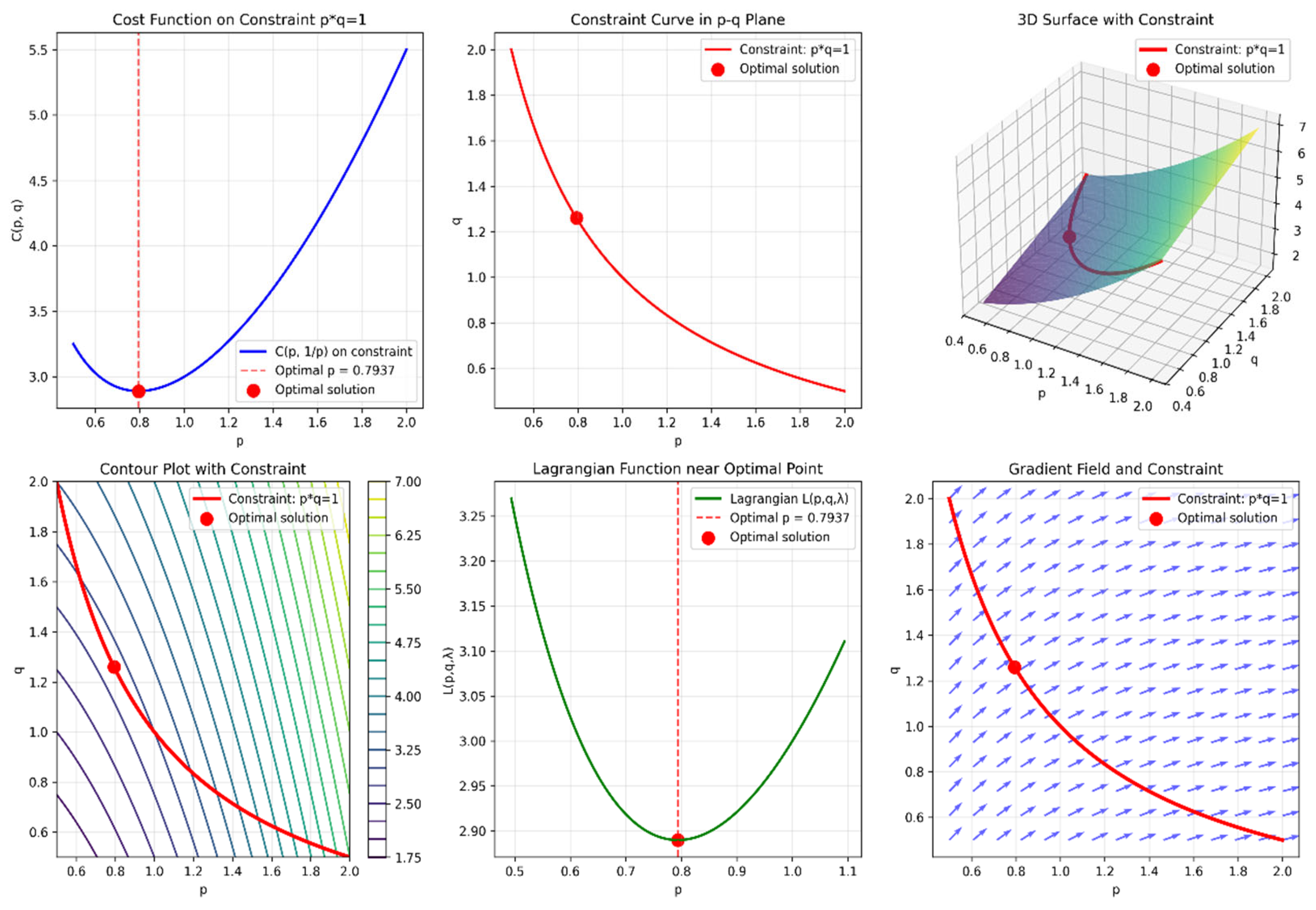
As can be seen from Figure 1, if the scale elasticity coefficients of the variables p and q in the constraint are equal and returns to scale are constant, then the optimal solution depends on the values of the elements of the Hessian matrix of the objective function. As clearly shown in Figure 1, near the optimal solution, the relationship between p and cost C is as follows: when the value of p exceeds the optimal p value (denoted as p*), the cost begins to increase at an accelerating rate. Additionally, it is observed that the p values on either side of the optimal solution are asymmetric. Specifically, when p is less than p*, cost C also rises at an accelerated rate, but this increase is faster than when p is greater than p*. From the perspective of input–output, this indicates that when the elasticity of inputs and outputs is equal or similar, marginal costs will rise more rapidly as educational input increases.
Next, let us examine the relationship between p and q: specifically, the scale substitution relationship. When p exceeds p*, the value of q gradually decreases. Focusing on the optimal solution, the q value exhibits significant asymmetry on either side of the optimal point. The rate of decline in q is faster on the left side than on the right side.
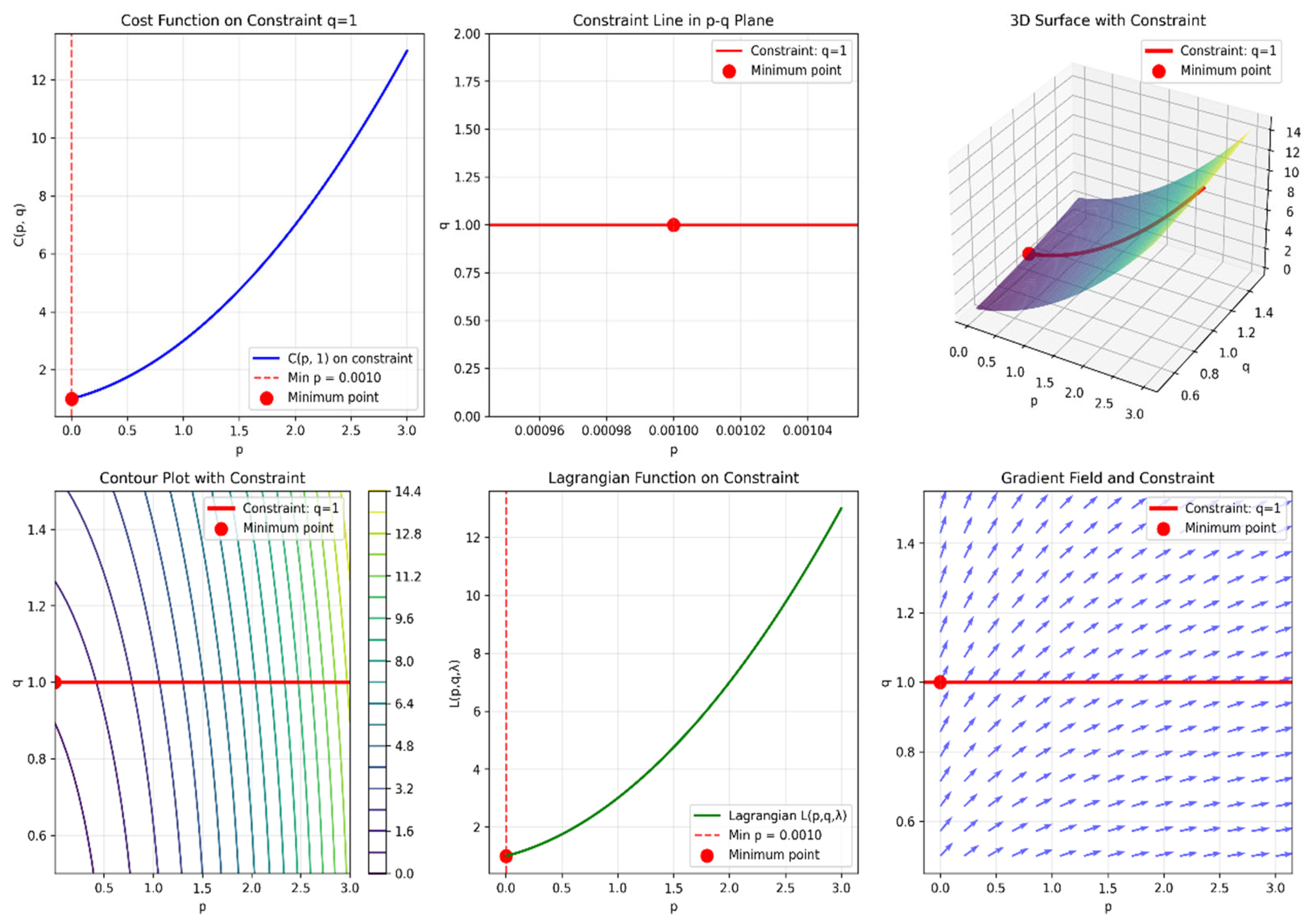
It can be seen from Figure 2 that if the elasticity coefficient of variable p in the constraint is much greater than that of q, and the returns to scale remain constant, then in the optimal solution, the value of p will be much smaller than that of q.
From Figure 2, it can be clearly seen that near the optimal solution, the relationship between p and cost C is as follows: when p is greater than p*, cost C will also accelerate its increase, and the rate of increase will become faster and faster. Next, let us take a look at the relationship between p and q, where q is essentially a horizontal line. From an economic perspective, if universities blindly expand their scale, it will result in a sharp increase in the total cost of education, which is not conducive to the long-term sustainable and stable development of universities.
As shown in Figure 3, if the variables p and q in the constraint have equal scale elasticity coefficients and the returns to scale are constant, then the objective function forms a spatial parabolic. In this case, the optimal solution of the problem depends on the equilibrium positions of p and q in the objective function, with the change in the value of p being slightly larger than that of q.
From Figure 3, it can be clearly seen that near the optimal solution, when p is greater than p* and gradually increases, the cost will gradually increase at a faster rate. At the same time, we can see that the value of p is not symmetrical on both sides of the optimal solution. That is to say, when p is less than p*, cost C will also increase at a faster rate than when p is greater than p*. From the perspective of input–output, the average cost of running a university will decrease with the increase in input–output in the initial stage, and then rise again after a period of time. Once the marginal cost exceeds the average cost, the increase in input–output will eventually offset the decrease in unit cost, leading to the depletion of economies of scale and the start of the unit cost increase.
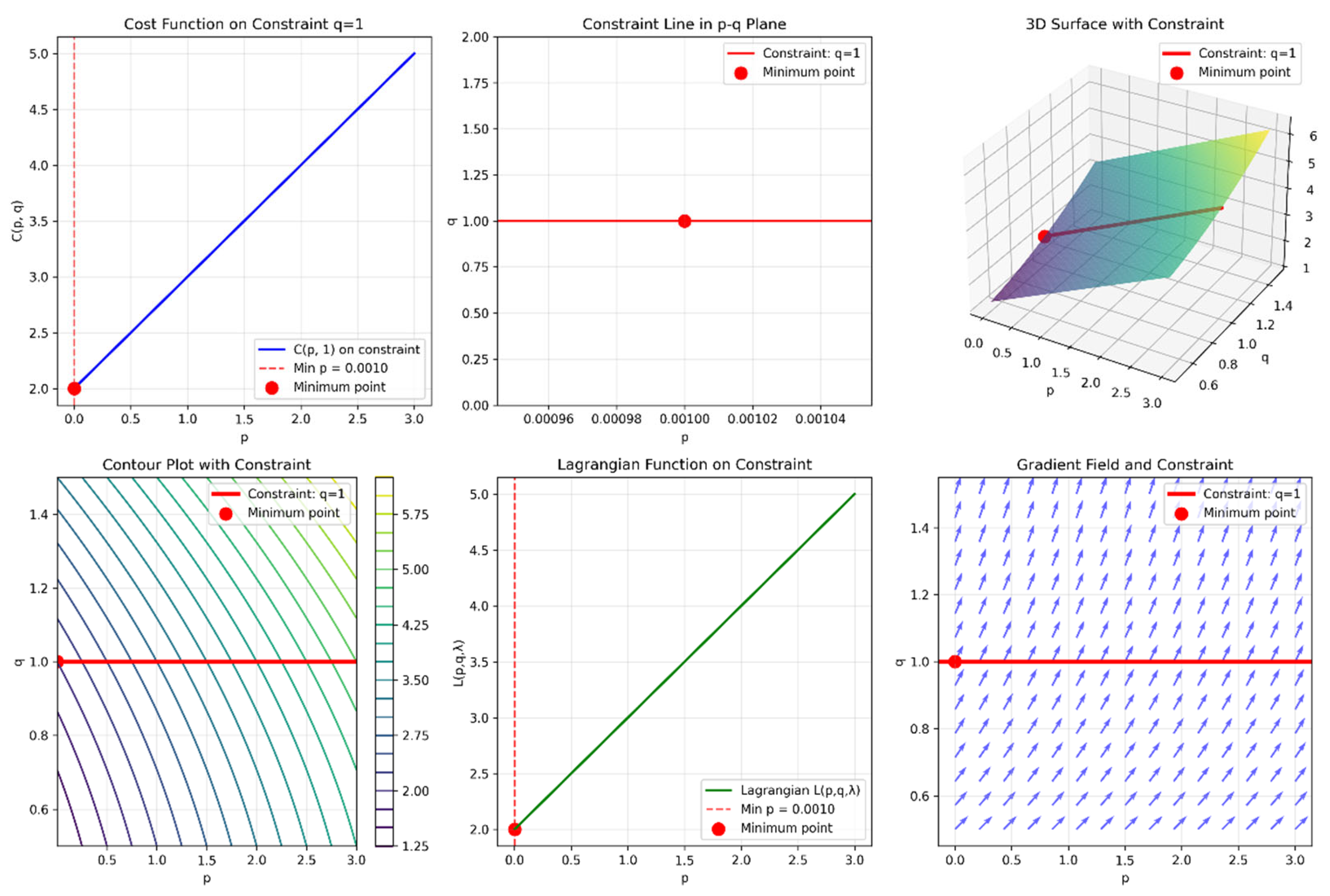
As can be seen in Figure 4, if the elasticity coefficient of the variable p in the constraint is much greater than that of q, and the returns to scale are constant, the objective function forms a parabolic surface in space, and in the optimal solution, the value of p is significantly smaller than that of q.
From the perspective of input–output, the average cost of running a college will decrease with the increase in input–output in the initial stage and then increase again after a period of time. Once the marginal cost exceeds the average cost, the increase in input–output will eventually offset the decrease in unit cost, leading to the depletion of economic scale and the start of unit cost increase. Next, let us take a look at the relationship between p and q, which is the relationship of scale substitution. When p is greater than p *, the value of q slowly decreases. If the optimal solution is taken as the center, the q value has significant asymmetry on both sides of the optimal solution. The rate of decrease in the q value is faster on the left side than on the right side.
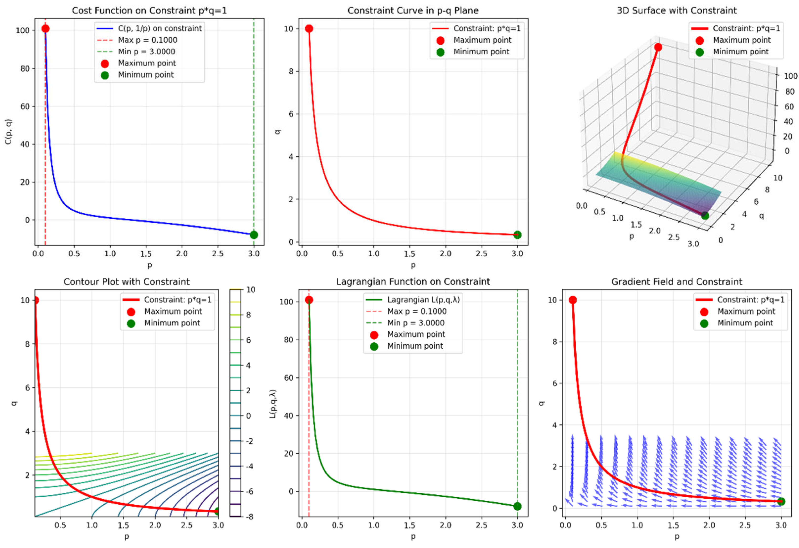
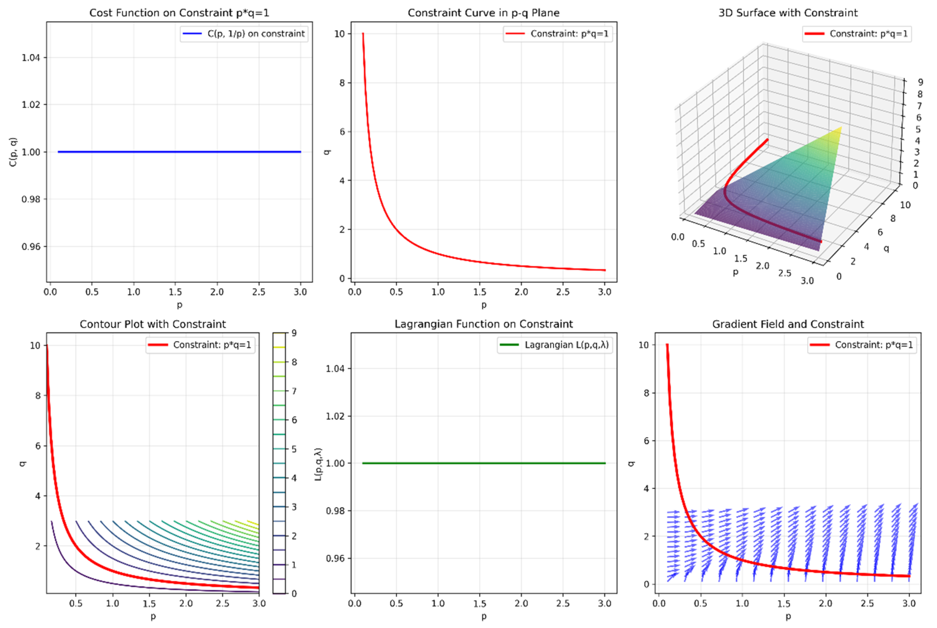
From Figure 5, we can see that if the scale elasticity coefficients of the variables p and q in the constraint are equal, and the returns to scale are constant, the objective function forms a hyperbolic surface in space. In this case, as the value of p decreases and q increases, the total cost increases rapidly.
It can be clearly seen from Figure 5 that near the optimal solution, the relationship between cost C and p is almost proportional: that is, the increase in cost C and the variable p increases, and the rate of increase remains unchanged. From an economic perspective, if universities are too focused on educational output, they will consume a large amount of educational resources, ultimately leading to a sharp increase in the total cost of running a university, making it difficult for universities to maintain high levels of educational output.
As can be seen from Figure 6, if the elasticity coefficient of the variable p in the constraint is much greater than that of q, and the returns to scale remain constant, the scenario represented by the objective function includes government subsidies and social donations, among others. Therefore, its optimal solution is relatively complex and requires further in-depth discussion.

4. Discussion

In this paper, we have analyzed the optimization of university costs from the perspective of the input–output theory. The conclusions drawn from the research are discussed in the following four aspects:
(1)
Qualitative division of costs through the input–output theory. When measuring from the scale of input and output of Chinese universities, universities in mainland China can roughly be divided into three input–output combinations: ‘low input–high output,’ ‘high input–low output,’ and ‘low input–low output.’ The concepts of ‘high’ and ‘low’ are only rough comparative classifications, and it can be seen from the regression results in the existing literature that the relationship between the levels of input–output combinations and the efficiency of the input–output is not very clear. In other words, universities that invest heavily in educational resources and incur high corresponding costs do not necessarily achieve output that meets expectations. In the past, schools that were judged to have high educational quality based on absolute input and output, as well as some traditional prestigious universities, often performed unsatisfactorily in terms of education input–output efficiency. At the same time, there are cases where institutions achieved higher-than-expected output with relatively low resource input, because the cost of running the school was minimized (resource allocation is optimized). This leads us to think that, in order to accurately assess the actual operational cost of a university, the government should pay attention to examining the efficiency of the educational input and output, rather than simply evaluating based on absolute amounts.
(2)
The existing statistical analysis data supports the two basic results of this paper. According to the results of the existing research [23], among the 51 universities directly under the Ministry of Education in China, 62.75% have high education input–output efficiency, 13.73% have relatively high education input–output efficiency and 23.52% have basically no efficiency in their education input–output. These analytical data indicate that more than half of the universities in mainland China have a relatively reasonable allocation of educational resources, but there are still a small number of universities with problems of excessively high costs. This paper has provided corresponding improvement methods for reference. The problem of excessively high costs in some universities mainly manifests as a redundant investment, most of which is concentrated in financial and human resources, especially financial investment, which is often made without regard to cost. Under the wave of expanding enrollment in major universities, some universities blindly pursue quantity, building large-scale high-ranking faculty teams, resulting in high costs and greatly wasting valuable educational resources. In some cases, even with high costs, universities still produce unsatisfactory educational outcomes, which is truly regrettable.
(3)
Universities should establish a complete evaluation index system for educational input–output efficiency. The shortcomings of the existing evaluation system are obvious to all. Optimizing the evaluation system can help identify various problems in the allocation and use of educational resources. At the same time, scientific and comprehensive evaluation methods should be used to study the education cost and input–output efficiency of universities. Interdisciplinary innovation should be sought in the selection of methods, with the goal of fundamentally solving problems.
(4)
At present, there is a common problem in the Chinese mainland’s colleges and universities: that the input of educational resources is redundant. Taking the construction of the teaching staff in the investment of educational resources as an example, the teaching staff is an important foundation for the development of education. However, in recent years, the blind expansion of education investment has brought huge “costs of tinkering” and waste, resulting in a surge in education costs [20]. In addition, it also occurs in terms of financial investment, where the budget for financial investment is not scientific enough and financial waste occurs repeatedly. These practical problems pose challenges for innovative research methods and specific practices in the future.
Future expansion: A worthwhile research direction in the future is to study cost issues from the perspective of the overall situation of universities, combining the structure and management of costs with the strategic development of universities. From a long-term strategic development perspective, cost optimization analysis and management control should be carried out to enhance the competitive advantage of the sustainable development of universities.

5. Conclusions

Scholars have long studied the cost of higher education. Yet, the current accounting system for colleges and universities lacks the capability for direct cost accounting, and a fully fledged, highly operable accounting system tailored to this context has yet to be established. Notably, the introduction of an accrual-based cost accounting method would provide a critical opportunity to revise universities’ accounting systems. To enhance the operability and effectiveness of higher education cost accounting, key issues—such as the object of cost accounting, cost accounting items and cost accounting methods—must first be addressed through targeted cost accounting practices.
According to the restrained condition of the Cobb–Douglas production function, all the colleges and universities try to do their best to find an optimal way to reach the minimum cost of higher education to maximize the efficiency of running a university. In other words, they can design the scientific allocation of input and output to the minimum cost of running a university.
When detH2 > 0, universities with such cost function characteristics emphasize both research and teaching, and they can be classified as research and teaching-oriented universities. When deciding on operating costs, these universities often choose a compromise asset allocation plan and strive to minimize the school’s operating costs through balance in various aspects; when detH2 = 0, universities with this type of cost function are teaching-oriented. They generally prefer asset allocation that benefits student development, thereby minimizing the overall operating costs of the university. When detH2 < 0, universities with this type of cost function are research-oriented. They tend to pursue higher university rankings and choose asset allocations that favor investment in research facilities, thereby minimizing the overall operating costs of the university.
In this paper, we selected a method combining the production functions theory and optimization theory to explore the cost minimization issue in the process of sustainable development in higher education institutions, particularly focusing on the multiple rounds of higher education reforms since the 1990s, such as mergers, enrollment expansions and the establishment of new campuses, where more than four-fifths of the universities evolved from a single campus to multiple campuses by merging and building new campuses. The system engineering triggered by the merger has fundamentally changed the operating costs of the merged higher education institutions directly under the Ministry of Education, with the most significant change being that the total expenditure per student increased sharply after the merger finished, driven first by an increase in salary and benefits per teacher and then by the expenditure per student for goods and services. An increase in the mergers of universities resulted in higher running costs; the heterogeneous merger of academic disciplines, the merger of those universities with great strength, and the merger of those universities not belonging to the centrally administered universities significantly increased the pressure on their running costs, and a longer geographical distance between the merged campus and the old campus resulted in higher running costs. According to the scale effect theory in economies, with the rapid expansion of enrollment in 1999, the total expenditure per student and the expenditure on goods and services declined rapidly, indicating a direct short-term result of the economies of scale. In short, the new campuses resulting from continuous enrollment expansion increased the total expenditure per student, of which the expenditure per student on infrastructure and equipment rose at first but declined later, and the expenditure per student on goods and services rose slightly. The new campuses built after the merger bore higher running costs and the new campuses built in a local university town could significantly reduce the running costs.

Author Contributions

Conceptualization, M.L.; Validation, Y.Y.; Formal analysis, Y.Y.; Investigation, M.L.; Resources, P.J.; Writing—original draft, M.L.; Funding acquisition, P.J. All authors have read and agreed to the published version of the manuscript.

Funding

This research was funded by the Ministry of Education (Grant number: 24JZDW008), the National Social Science Foundation (Grant number: 21FJKB012) and the Chinese Society of Higher Education (Grant Number 23SX0205).

Data Availability Statement

The original contributions presented in this study are included in the article. Further inquiries can be directed to the corresponding author.

Conflicts of Interest

The authors declare no conflicts of interest.

References

  1. Price, J.A. How cost framing affects college applications: Evidence from a targeted information intervention. Econ. Educ. Rev. 2025, 107, 102677. [Google Scholar] [CrossRef]
  2. Gajderowicz, T.; Wincenciak, L.; Grotkowska, G. How much does a higher education in economics cost? DCE evaluation of the individual (dis)utility of studying. Int. Rev. Econ. Educ. 2024, 47, 100294. [Google Scholar] [CrossRef]
  3. Chao, L. Research on full cost accounting in Sino-foreign cooperative education institutions in universities: A Case study of T university. Money China 2023, 34, 84–86. [Google Scholar]
  4. Schouten, J.; Saavedra-Nieves, A.; Fiestras-Janeiro, M.G. Sequencing situations and games with non-linear cost functions under optimal order consistency. Eur. J. Oper. Res. 2021, 294, 734–745. [Google Scholar] [CrossRef]
  5. Gomez, M.A.; Michiels, W.; Mondié, S. Design of delay-based output-feedback controllers optimizing a quadratic cost function via the delay Lyapunov matrix. Automatica 2019, 107, 146–153. [Google Scholar] [CrossRef]
  6. Rebello, G.; Gondhalekar, R.; Dassau, E.; Doyle, F.J., III. Mixed Linear-quadratic cost function design for MPC of an artificial pancreas—improved treatment & safety for a broad range of meal sizes. IFAC-PapersOnLine 2017, 50, 7724–7730. [Google Scholar]
  7. Hongyi, T. Research on compliance governance of affiliated transaction in private universities. Heilongjiang High. Educ. Res. 2023, 41, 39–43. [Google Scholar]
  8. Guiyan, C.; Mingda, L.; Shuang, H.; Zhanli, M.; Jingchao, C. Research on the financial accounting reporting system of Sino-foreign cooperative education in universities from the perspective of Full-cost accounting: A case study of M university. Stud. Financ. Account. Educ. 2022, 33, 54–62. [Google Scholar]
  9. Oskarsson, B. Total cost analysis in purchasing education: A two-step open-ended teaching case approach. J. Purch. Supply Manag. 2025, 31, 100971. [Google Scholar] [CrossRef]
  10. Glass, J.C.; McKillop, D.G.; Hyndman, N.S. Efficiency in the provision of university teaching and research: An empirical analysis of UK universities. J. Appl. Econom. 1995, 10, 61–72. [Google Scholar] [CrossRef]
  11. Kim, J.; Nakano, S.; Nishimura, K. Multifactor CES general equilibrium: Models and applications. Econ. Model. 2017, 63, 115–127. [Google Scholar] [CrossRef]
  12. Baumol, W.J.; Panzar, J.C.; Willig, R.D. Contestable Markets and the Theory of Industry Structure; Harcourt Brace Jovanovich: San Diego, CA, USA, 1982. [Google Scholar]
  13. Zhang, X.; Sun, D.; Jiang, W. Dynamics of ahet erogeneous quantumcournot duopoly with adjusting players and quadratic costs. Quantum Inf. Process. 2020, 19, 403. [Google Scholar] [CrossRef]
  14. Feiyu, Z.; Huisheng, Z.; Jian, W. A widely linear noise-constrained adaptive filtering algorithm with a non-quadratic cost function. Digit. Signal Process. 2025, 165, 105333. [Google Scholar] [CrossRef]
  15. Azioune, M.; Abdelouahab, M.S. Controlling chaos and mixed mode oscillations in a Bertrand duopoly game with homogeneous expectations and quadratic cost functions. Math. Comput. Simul. 2025, 233, 553–566. [Google Scholar] [CrossRef]
  16. Yong, D.; Hanlei, W.; Wei, R. Distributed continuous-time time-varying optimization for networked Lagrangian systems with quadratic cost functions. Automatica 2025, 171, 111882. [Google Scholar] [CrossRef]
  17. Johnes, G. Multiproduct cost functions and the funding of tuition in UK universities. Appl. Econ. Lett. 1996, 3, 557–561. [Google Scholar] [CrossRef]
  18. Mian, A.; Ensinas, A.V.; Marechal, F. Multi-objective optimization of SNG production from microalgae through hydrothermal gasification. Comput. Chem. Eng. 2015, 76, 170–183. [Google Scholar] [CrossRef]
  19. Yu, B.Z.; Lu, M.X. Analysis for a Sort of Higher Education Cost from the View at Constrain of Cobb-Douglas function. In Proceedings of the ICBDIE, Beijing, China, 8–10 April 2022. [Google Scholar]
  20. Wang, L. Empirical Estimate of Education Cost Function for University and Its Application. Master’s Thesis, Suzhou University, Suzhou, China, 2009. [Google Scholar]
  21. Boyd, S.P.; Vandenberghe, L. Convex Optimization; Cambridge University Press: Cambridge, UK, 2004. [Google Scholar]
  22. Horn, R.A.; Johnson, C.R. Matrix Analysis; Cambridge University Press: Cambridge, UK, 2012. [Google Scholar]
  23. Jin, L. A Study on the Measurement of Input-Output Efficiency of Higher Education in China Based on Comprehensive Evaluation Method. Master’s Thesis, Jinan University, Guangzhou, China, 2019. [Google Scholar] [CrossRef]
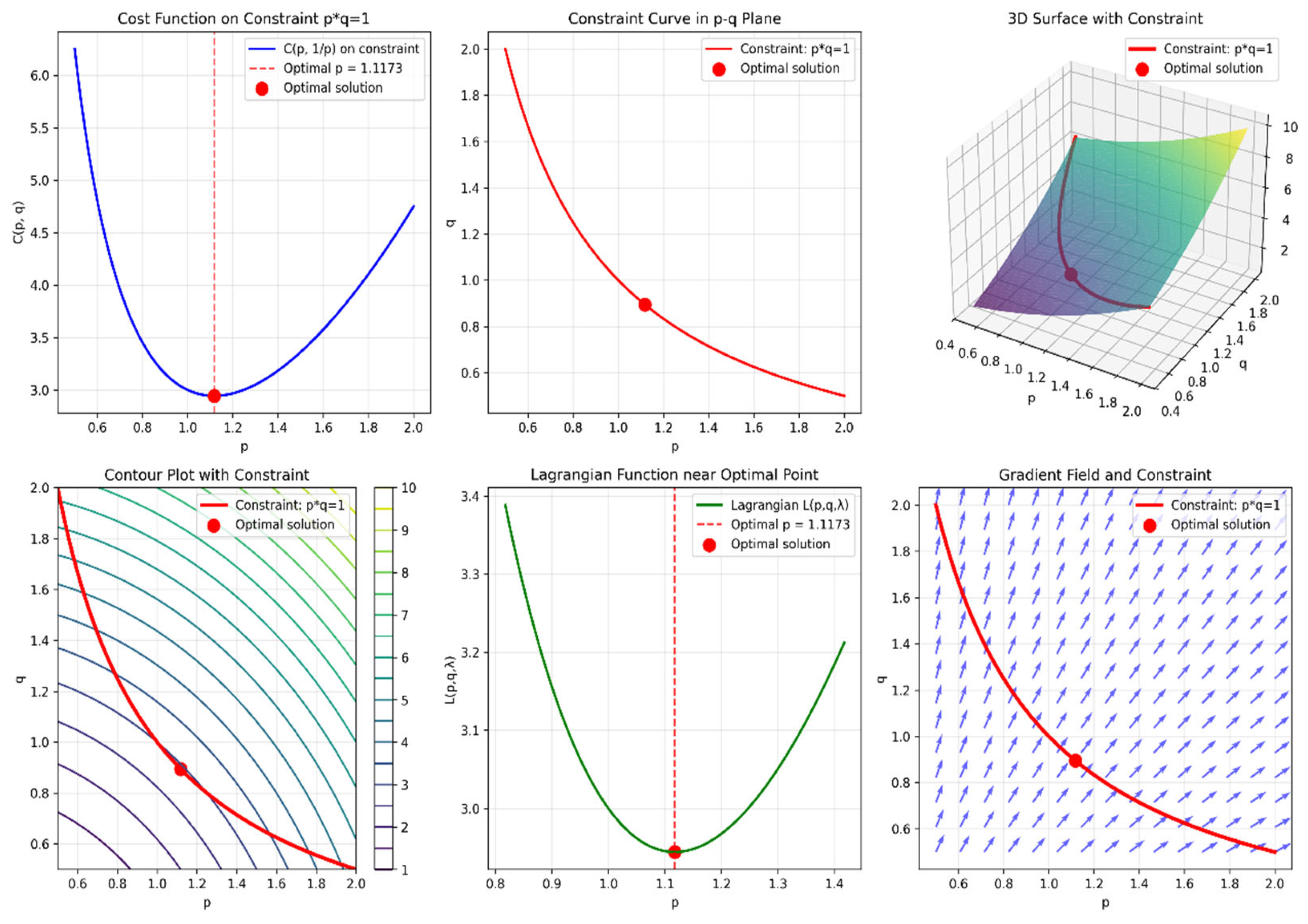
Figure 1. detH2 > 0, a = b = 0.5.
Symmetry 17 02035 g001
Figure 2. detH2 > 0, a = 1,b = 0.
Symmetry 17 02035 g002
Figure 3. detH2 = 0, a = b = 0.5.
Symmetry 17 02035 g003
Figure 4. detH2 = 0, a = 1, b = 0.
Symmetry 17 02035 g004
Figure 5. detH2 < 0, a = b = 0.5.
Symmetry 17 02035 g005
Figure 6. detH2 < 0, a = 1, b = 0.
Symmetry 17 02035 g006
Table 1. Definition of parameters.
SymbolParameter Definition
α k the amount of total cost change that is caused by the price of the kth product of the input product increasing by one unit.
β i the amount of total cost change that was caused by the price of the ith product of the output product increasing by one unit.
δ k l the price relationship coefficient between product k and product l of input products.
γ k l the price relationship coefficient between product k and product l of output products.
ρ k i the price relationship coefficient between input product k and input product i.
c 0 the sum of financial support that universities can provide for all input and output production and external resources of universities.
a k the amount of the kth input product.
b i the amount of the ith output product.
Disclaimer/Publisher’s Note: The statements, opinions and data contained in all publications are solely those of the individual author(s) and contributor(s) and not of MDPI and/or the editor(s). MDPI and/or the editor(s) disclaim responsibility for any injury to people or property resulting from any ideas, methods, instructions or products referred to in the content.