Article

A Symmetric Deep Learning Approach for Dynamic Reserve Evaluation of Tight Sandstone Gas Wells

1
College of Petroleum Engineering, Xi’an Shiyou University, Xi’an 710065, China
2
PetroChina Company Limited Daqing Oilfield Company, Daqing 163453, China
3
PetroChina Company Limited Changqing Oilfield Company, Yulin 719000, China
*
Author to whom correspondence should be addressed.
Symmetry 2025, 17(12), 2033; https://doi.org/10.3390/sym17122033 (registering DOI)
Submission received: 14 October 2025 / Revised: 11 November 2025 / Accepted: 19 November 2025 / Published: 28 November 2025
(This article belongs to the Section Computer)

Abstract

Traditional dynamic storage calculation methods face challenges such as difficult data acquisition and prolonged testing periods. To address the industry’s need for rapid yet accurate estimation of single-well dynamic reserves in tight sandstone gas formations, a deep learning architecture combining convolutional neural network (CNN) and long short-term memory (LSTM) network is proposed. This model enables fast and accurate reserve evaluation, outperforming other machine learning methods in overall capability while achieving a symmetric improvement in both training efficiency and prediction accuracy—reaching up to 95.9%. Based on this model, dynamic reserves of gas wells in the Sulige Gas Field were predicted. The single-well dynamic reserve test showed a relative error of less than 10%, and the method demonstrated strong stability and high precision in localized multi-well group tests, with errors distributed symmetrically within a narrow margin. All results satisfy engineering standards. The feasibility of the method has been verified, proving it can deliver fast and accurate gas well dynamic reserve predictions, greatly reduce evaluation costs, and enhance work efficiency.

1. Introduction

Currently, global energy consumption continues to rise. A persistent upward trend has been observed in the demand for oil and natural gas, which remain core fossil fuels. Having been exploited for centuries, the decline of conventional oil and gas reservoirs is becoming increasingly evident, whereas unconventional resources present considerable potential for future development. Tight sandstone gas, a significant unconventional oil and gas resource, has entered a phase of rapid expansion. According to 2022 data, unconventional natural gas contributed 41% (912 × 108 m3) to China’s total gas output, of which tight gas constituted a significant portion of 57.6 × 10⁸ m3 [1,2]. However, the dynamic reserve assessment of such reservoirs is highly challenging due to their pronounced heterogeneity, low productivity per well, and complex gas–water interactions, which pose a major challenge to conventional evaluation methods [3,4,5].
The accurate prediction of dynamic reserves constitutes the foundation for efficient gas well development, guiding critical decisions from initial design to subsequent production optimization [6,7,8,9]. Conventional assessment methods mainly include the material balance method, empirical analysis method, modern production instability analysis method, and well testing method [10,11,12,13,14]. The material balance method is applicable to various gas reservoirs but requires high accuracy in pressure data [15]. The empirical analysis method is relatively simple, but there is greater uncertainty when data is scarce [13]. The well testing method requires high-precision pressure test data [16,17]. The modern production instability analysis method has a wide adaptability and low pressure requirements [18,19,20,21], but it requires high accuracy and completeness of historical well data. The above methods either focus on calculating high accuracy or reducing workload. A central technical challenge currently lies in developing dynamic reserve prediction methods that simultaneously achieve both computational efficiency and predictive accuracy across diverse gas well types.
In recent years, the rapid advancement of artificial intelligence has opened up new avenues for dynamic reserve prediction through machine learning approaches [22,23,24,25]. Compared with conventional methods, this method establishes a prediction model through data mining, which can quickly and accurately evaluate dynamic reserves. Minaizhe et al. [26] successfully predicted the recoverable reserves of gas wells by combining the gray relational analysis method and the BP neural network. The gray relational analysis method was used to screen key factors, and the BP neural network was used to build the prediction model. Fan Dongyan et al. [27] classified time series production dynamic data into strongly correlated and weakly correlated sequences based on Euclidean distance and used machine learning methods to predict different sequences. The prediction accuracy of strongly correlated sequences was good. Liu et al. [28] established a dynamic reserve prediction model using deep learning feedforward neural networks, integrating multiple factors including geology, engineering, and production parameters.
This paper builds upon a solid foundation of prior research and abundant multi-dimensional dynamic production data from the field. Its core content involves employing advanced deep learning technology to construct a dynamic reserve prediction and evaluation method specifically for tight gas wells. This research not only achieves accurate prediction of dynamic reserves in single wells but also establishes a complete methodological system from data processing to model application. Its ultimate goal is to provide a scientific basis and data-driven guidance for key decisions such as optimizing development plans and adjusting production systems in tight gas fields.

2. Dynamic Reserve Prediction Model

Machine learning has found extensive utility in the upstream oil and gas sector, with applications encompassing seismic interpretation, reservoir identification, production prediction, and development scheme optimization. A core factor in this trend is that machine learning algorithms are particularly adept at mining and establishing complex nonlinear relationships from massive amounts of data [22,29]. Based on this technological background and current development status, this paper innovatively proposes an organic combination of machine learning and modern production analysis methods to achieve rapid and accurate prediction of dynamic reserves in tight gas wells. Ultimately, this paper successfully constructed a new method specifically for dynamic reserve assessment of tight sandstone gas wells.
This study proposes a CNN-LSTM deep learning model designed to enhance the accuracy of dynamic reserve prediction for tight gas wells. Capitalizing on the local feature extraction of CNN and the temporal modeling of LSTM, this model harnesses these complementary strengths to build a hierarchical learning architecture. The corresponding prediction process is presented in Figure 1.

2.1. Convolutional Neural Network (CNN)

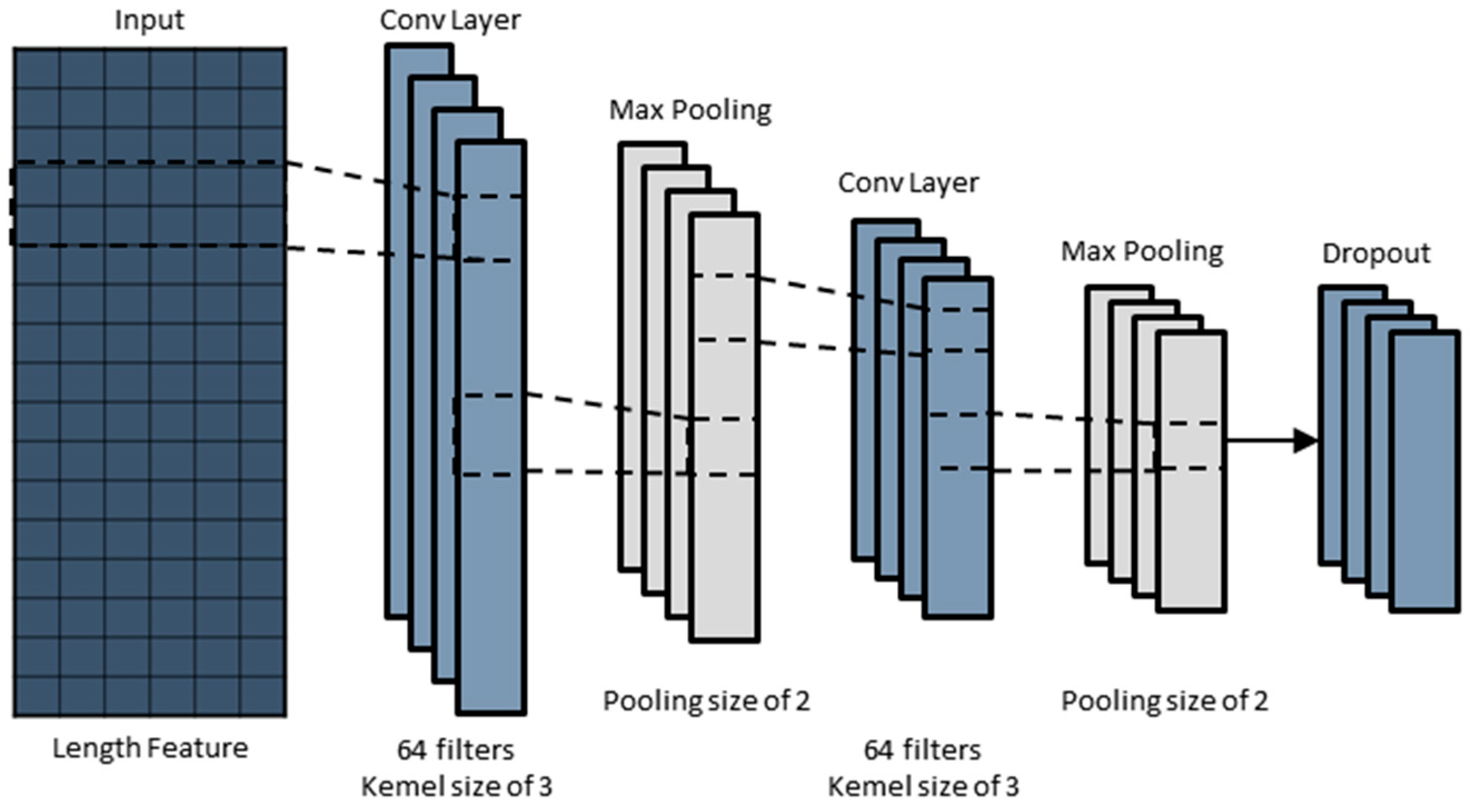
CNNs stand out among numerous neural network models due to their unique design of sparse connections and weight sharing. These characteristics enable them to maintain high computational efficiency while possessing excellent generalization capabilities and powerful hierarchical feature extraction performance [30]. As a feedforward neural network based on convolutional operations, its standard structure includes an input layer, an output layer, and complex hidden layers composed of convolutional, pooling, and fully connected layers. A one-dimensional CNN structure (as shown in Figure 2) is extensively used for time series and regression problems.

2.2. Long Short-Term Memory Neural (LSTM) Network

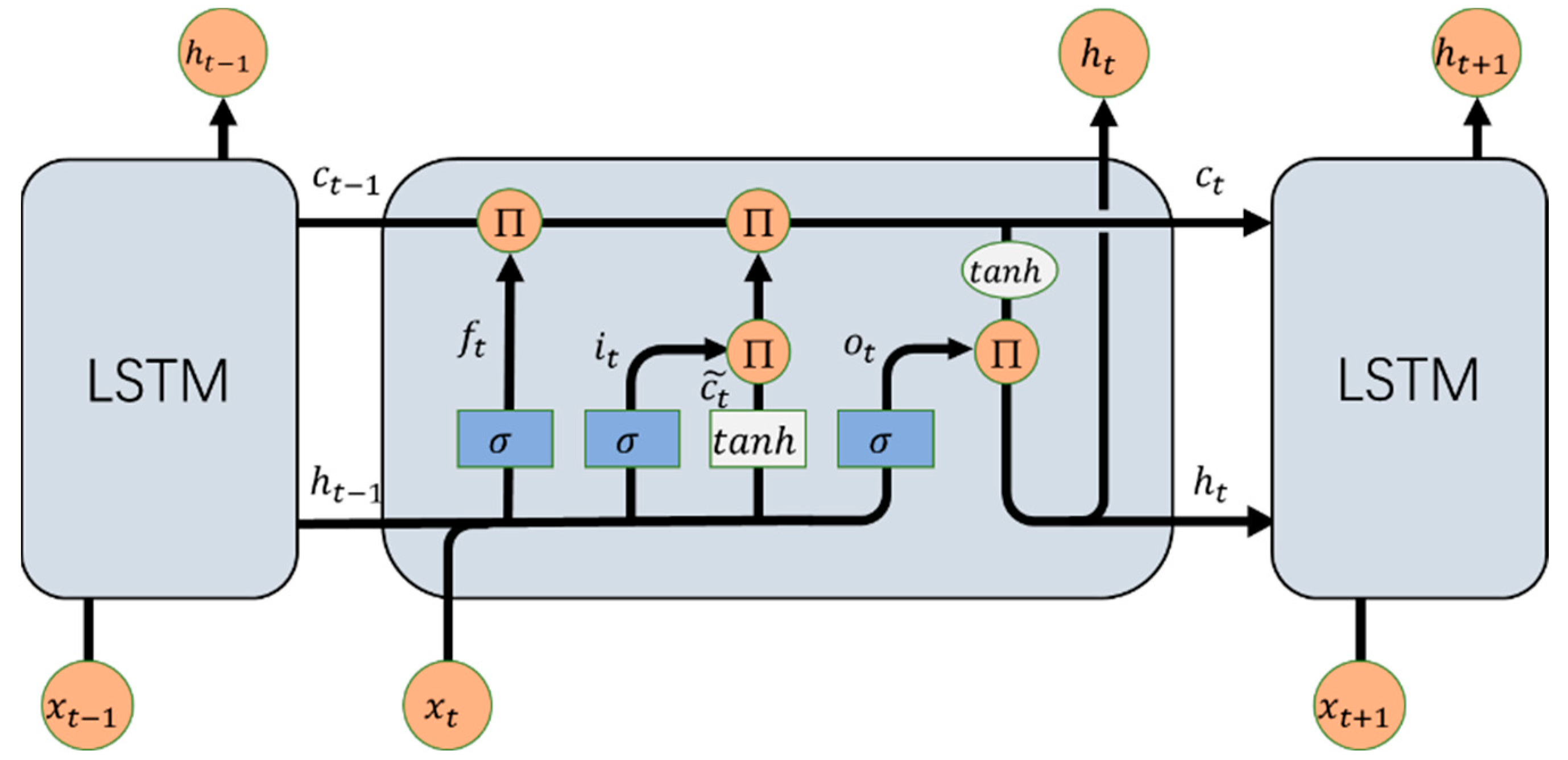
LSTM is a specialized type of recurrent neural network (RNN) designed to learn long-term dependencies. An LSTM network’s basic structure consists of an input layer, a core LSTM layer, and an output layer. Its key feature is within the LSTM layer, which is characterized by memory units and three dedicated gates (forget, input, and output) [31,32]. The architecture of the LSTM recurrent neural network is depicted in Figure 3. Leveraging its memory cells and gates, LSTM possesses the capability to capture long-range patterns in sequential data while simultaneously stabilizing gradient flow through dynamic information control, thereby effectively resolving the vanishing and exploding gradient problems.

2.3. CNN-LSTM Model

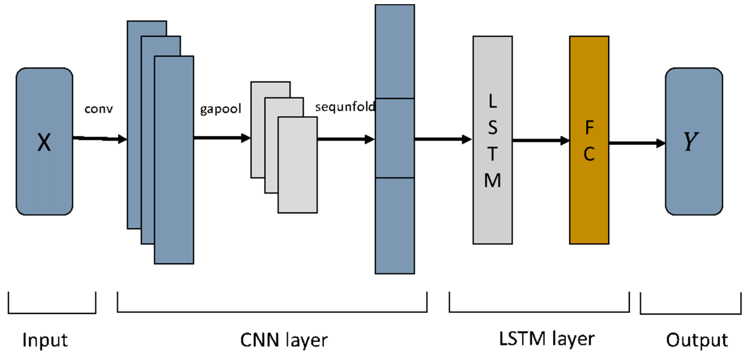
CNN and LSTM each specialize in different types of feature extraction. CNN is well-suited for local feature detection, while LSTM is particularly effective at capturing temporal dependencies in sequential data. This article proposes a CNN-LSTM combined model prediction method based on CNN and LSTM deep learning algorithms, as shown in Figure 4. The CNN layer extracts local features of the data, while the LSTM layer captures the dependencies between time series. The extracted features are fed into a fully connected layer, which is employed to compute the final regression value, thereby predicting the dynamic reserves at the next time step.

3. Data Collection and Experimental Setup

3.1. Information on the Research Area

Focusing on a typical tight sandstone gas reservoir exhibiting the common traits of low permeability, low pressure, and low abundance, this study is conducted in the eastern region of the Ordos Basin’s Sulige gas field. The reservoir exhibits a considerable burial depth, approximately 3500 m, and a thin single layer, ranging from 1.9 to 8.2 m. Its core physical parameters, including a low porosity of 5% to 14%, an extremely low permeability of 0.14 to 7.08 × 10⁻³ μm2, and a low gas saturation of only 28.6% to 29%, together form an extremely dense reservoir space. The dynamic reserve of a single well is a complex variable influenced by both dynamic production parameters and static geological parameters. Therefore, under such complex and uncertain conditions, establishing a dynamic reserve prediction model capable of integrating and accurately interpreting multi-source information is crucial for scientifically guiding development decisions and ultimately achieving the efficient development of tight gas resources. This study selected 150 wells in the research area of Sulige Gas Field that had completed dynamic reserve calculation using conventional methods and possessed complete data to serve as learning and training samples.

3.2. Data Acquisition and Processing

The sample data includes 1 set of characteristic parameters, namely production time, pre-production casing pressure, porosity, gas saturation, permeability, single-layer effective thickness, cumulative gas production, daily gas production, formation pressure, casing pressure and tubing pressure (Table 1). The dimensions of different dynamic and static parameters are different, and the range of values varies greatly. To achieve comparability between different parameters and dynamic reserves, the study adopted a deviation normalization method to uniformly scale all well data to the [0,1] interval, thereby eliminating the influence of dimensions and bringing the data to a consistent level.
The corresponding normalization could be calculated by Equation (1).
X = X i X m i n X m a x X m i n
In the formula: X is the normalized data; X m a x and X m i n are the maximum and minimum values of the input dataset X i .

3.3. Correlation Analysis

To identify key features and clarify the relationship between parameters and dynamic reserves, a Pearson correlation analysis was conducted. This step was crucial for screening input variables and improving the subsequent prediction accuracy of the model.
The strength of a linear association between two features is measured by the Pearson correlation coefficient, which is bounded between −1 and 1. The Pearson coefficient’s sign indicates the direction of the correlation, with positive and negative values representing positive and negative relationships, respectively. Meanwhile, its absolute value, ranging from 0 to 1, quantifies the strength of the linear relationship, where values closer to 1 signify stronger associations.
The calculation formula for the Pearson correlation coefficient is as follows:
p x , y = i = 1 n x i x ¯ y i y ¯ i = 1 n x i x ¯ 2 i = 1 n y i y ¯ 2
In the equation, p ( x , y ) is the Pearson correlation coefficient; x ¯ is the average value of each feature parameter; y ¯ is the average value of the target parameter.
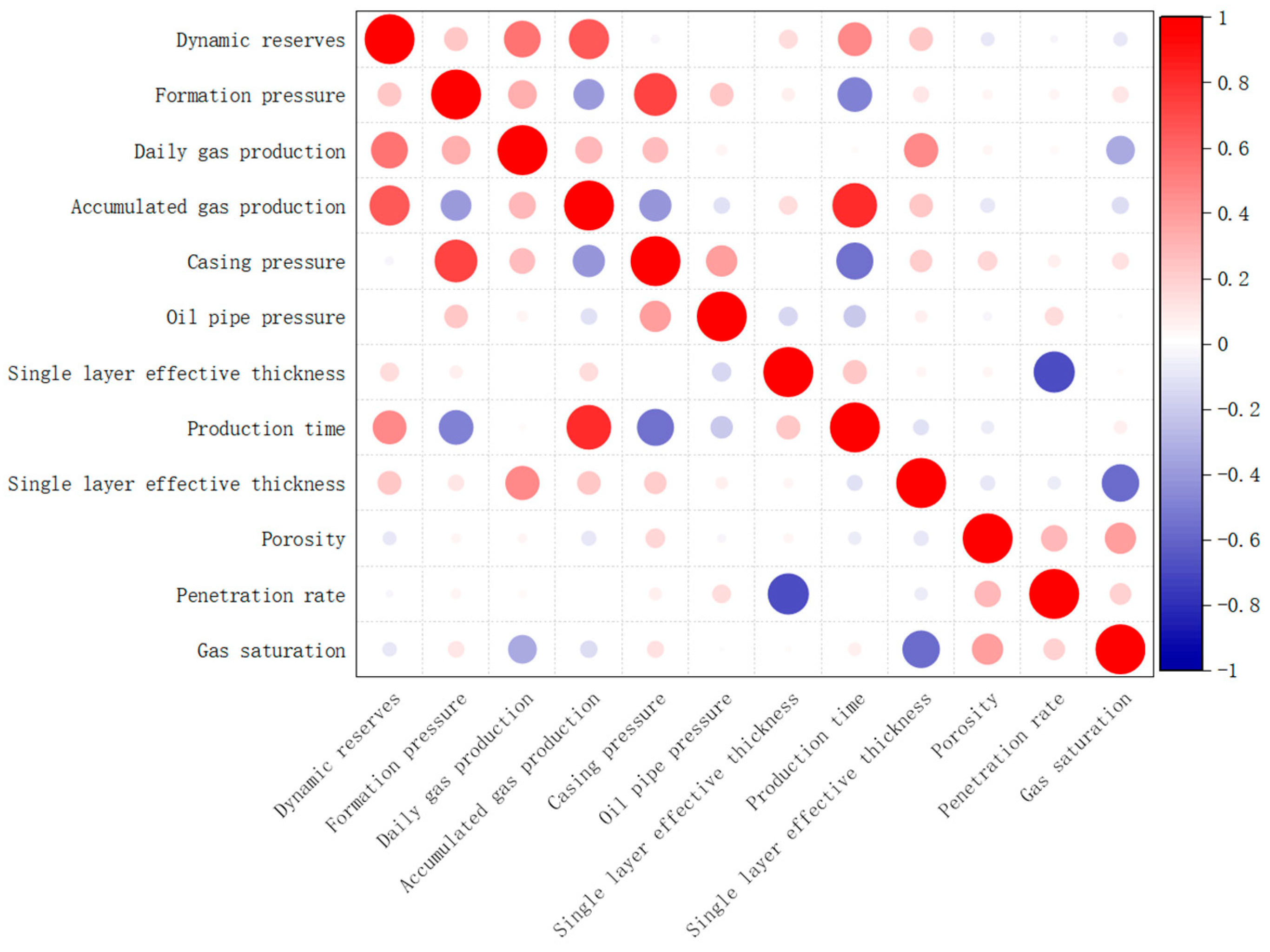
The correlation coefficients obtained using the Pearson correlation coefficient method are shown in Figure 5. It can be seen that cumulative gas production, daily gas production, production time, cumulative effective thickness, formation pressure, pre-production casing pressure, and tubing pressure are positively correlated with dynamic reserves, while gas saturation, porosity, casing pressure, and permeability are negatively correlated with dynamic reserves. Dynamic reserves exhibit a significant linear dependence on dynamic parameters, including cumulative and daily gas production. Conversely, the relationship with static parameters, such as porosity and permeability, is governed by a complex nonlinear association.

3.4. Construction of Deep Learning Prediction Models

Employing the coefficient of determination (R2), mean absolute error (MAE), root mean square error (RMSE), and mean absolute percentage error (MAPE), we rigorously assessed the prediction accuracy of the dynamic reserve model to verify its practical reliability.
The specific formula is as follows:
R 2 = 1 i = 1 n f x i x i 2 i = 1 n f x i x i ¯ 2
M A E = 1 n i = 1 n f x i x i
R M S E = 1 n i = 1 n f x i x i 2
M A P E = 1 n i = 1 n f x i x i x i
In the formula: f x i is the predicted value of dynamic reserves for a single well; x i is the true value; x i ¯ is the average value.

4. Example Application

4.1. Model Parameter Settings

In the prediction model of this paper, CNN and LSTM are connected in series in sequence. The dataset was partitioned into training and testing subsets with a ratio of 7:3. The CNN employs two convolutional layers, each containing 32 filters of 3 × 1 dimensionality, to extract spatial features from input data. The architecture utilizes ReLU activation functions and incorporates 2 × 1 max pooling operations for dimensional reduction. Feature maps generated by the CNN are subsequently flattened through a sequence unrolling layer and fed into the LSTM module. The LSTM network consists of two layers with 128 hidden units, implementing a 20% dropout rate. The model was trained over 1000 rounds with 3 iterations per round, using the Adam optimization algorithm with an initial learning rate of 0.01.

4.2. Analysis of Model Prediction Results

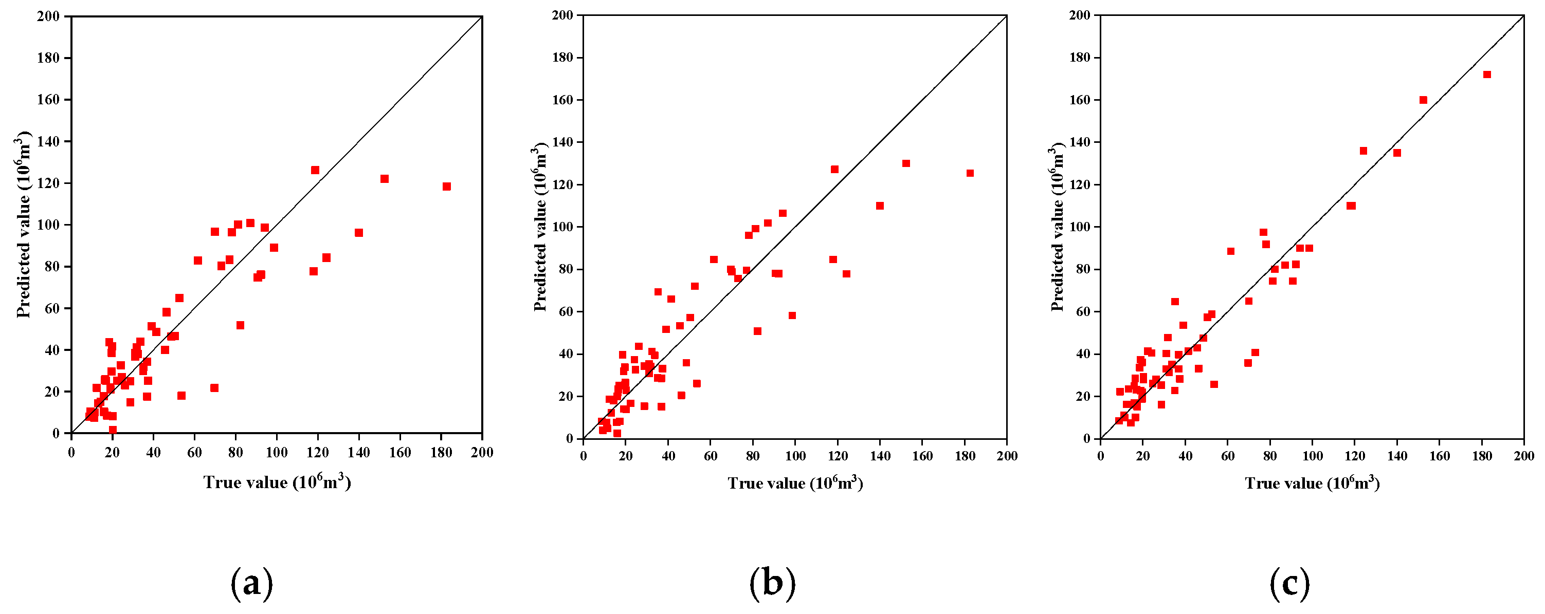
In order to compare the influence of different models and different combinations of feature parameters on dynamic reserve prediction, CNN, LSTM and CNN-LSTM deep learning models were constructed for dynamic reserve prediction, respectively. Figure 6 and Table 2 are performance comparison charts of different model test sets. While the CNN and LSTM models demonstrate a high level of agreement in their dynamic reserve predictions for the majority of cases, both exhibit pronounced errors when forecasting the maximum value of dynamic reserves. In contrast, the CNN-LSTM model can better capture data features and show smaller errors, and the prediction result accuracy is significantly improved compared with CNN and LSTM. The determination coefficient R2 predicted by the CNN-LSTM model is 0.959.

4.3. Comparative Experiment

To verify the accuracy of the CNN-LSTM model proposed in this paper, we further compared it with various classic machine learning methods, including decision trees, support vector machines, linear regression, and BP neural network models. Table 3 presents the results obtained from the different models.
As presented in Table 3, the coefficients of determination for both BP and CNN-LSTM models exceed the threshold of 0.8. The determination coefficient of the CNN-LSTM model in this paper far exceeds that of other similar machine learning methods. The results of comparative analysis prove that the CNN-LSTM model can predict dynamic reserves well and is far superior to other machine learning methods.

4.4. Practical Applications

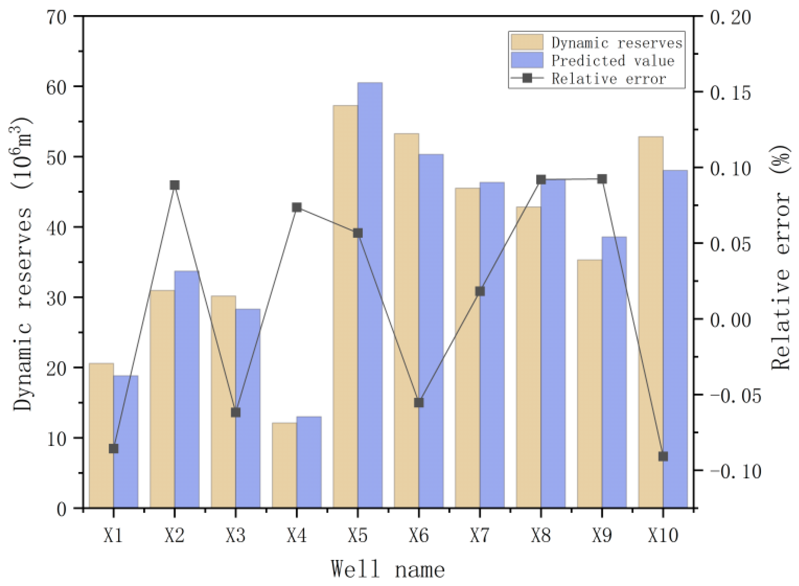
To further verify the predictive performance of the model, data from 10 wells that did not participate in the model training were re-collected in the study area and brought into the CNN-LSTM for training. For the newly selected wells, a certain level of relative error is observed between the model’s predictions and the actual dynamic reserves, as evidenced in Figure 7. Specifically, the relative error for all samples is controlled within a narrow range of −9.08% to 9.23%. This indicates that the model has good extrapolation accuracy and robustness, and its prediction error is strictly limited to a low, engineering-acceptable range. To further verify the accuracy and applicability of the dynamic reserve prediction model for tight gas wells based on deep learning.
A significant trend in tight gas field development is characterized by a swift increase in the number of development wells. This has subsequently led to more complex well network structures and increased interference between individual wells. Traditional dynamic reserve calculation methods based on isolated wells or simple well networks have become significantly less applicable under these complex conditions. Therefore, how to conduct accurate reserve assessment in this new development environment has become a pressing technical challenge. A validation study was conducted by training the model on data from 30 adjacent wells within the research area, aiming to verify its performance in predicting dynamic reserves for localized multi-well groups. The result is shown in Figure 8. It shows high accuracy in dynamic reserves prediction of multi-well groups.
Practice has proven that this deep learning model has practical application potential in the field of dynamic reserve prediction. One important application is its use in single wells within the study area that lack historical production data and have not yet undergone traditional assessments, enabling the rapid acquisition of their dynamic reserve estimates. This effectively fills the gaps in traditional methods, providing direct and quantitative data support for target selection, production capacity development, and investment decisions for these single wells.

5. Conclusions

(1)
To address the industry bottleneck in dynamic reserve assessment of low-permeability tight gas wells, an innovative deep learning technology approach combining CNN and LSTM was adopted. By leveraging on-site dynamic and static data, this model offers a solution for the fast and precise estimation of gas well dynamic reserves, providing a new technique for tight gas reservoir evaluation.
(2)
The results of the instance test show that the R2 predicted by the CNN-LSTM model reaches 0.959. This accuracy is markedly higher than that achieved by traditional machine learning models such as the individual CNN and LSTM architectures.
(3)
The application results show that the relative error of the single-well dynamic reserves prediction test is less than 10%, and it shows good stability and high accuracy in the dynamic reserves prediction test of adjacent multi-well groups in a small range, and the calculation results meet the engineering requirements.

Author Contributions

Conceptualization and Supervision, Y.Z.; Writing—original draft, B.Z.; Investigation, B.L.; Methodology, H.Z.; Resources, J.B.; Resources, X.T.; Data curation, P.L.; Validation, J.W.; Software and Visualization, P.L.; Software and Visualization, C.F. All authors have read and agreed to the published version of the manuscript.

Funding

This research was funded by Deep Earth Probe and Mineral Resources Exploration—National Science and Technology Major Project, grant number 2024ZD1004406.

Data Availability Statement

The original contributions presented in this study are included in the article. Further inquiries can be directed to the corresponding author.

Conflicts of Interest

Authors Liu Banghua and Bai Junhui were employed by the PetroChina Company Limited Daqing Oilfield Company, and Tian Xijun and Liu Peng were employed by the PetroChina Company Limited Changqing Oilfield Company. The remaining authors declare that the research was conducted in the absence of any commercial or financial relationships that could be construed as a potential conflict of interest.

References

  1. Zou, C.; Lin, M.; Ma, F.; Liu, H.; Yang, Z.; Zhang, G.; Yang, Y.; Guan, C.; Liang, Y.; Wang, Y.; et al. Progress, challenges and countermeasures of China’s natural gas industry under the goal of carbon neutrality. Pet. Explor. Dev. 2024, 51, 418–435. [Google Scholar] [CrossRef]
  2. Oil and Gas Department of National Energy Administration; Resource and Environmental Policy Research Institute of the Development Research Center of the State Council; Oil and Gas Resources Strategic Research Center of the Ministry of Natural Resources. Natural Gas Development Report of China; Petroleum Industry Press: Beijing, China, 2023. [Google Scholar]
  3. Cheng, M.; Lei, D.; Zhang, L.; Liu, L.; Zhao, M. Technical strategy for beneficial development of tight sand gas in Sulige Gas Field. Pet. Reserv. Eval. Dev. 2024, 14, 475–483. [Google Scholar] [CrossRef]
  4. Gao, Y.; Wang, B.; Hu, Y.; Gao, Y.; Hu, A. Development of China’s natural gas: Review 2023 and outlook 2024. Nat. Gas Ind. 2024, 44, 166–177. [Google Scholar] [CrossRef]
  5. Zhang, Y.; Li, X.; Yang, S.; Qiang, K.; Zhang, B.; Liu, J.; Wei, Q.; Wang, R. Research on Intelligent Production Optimization of Low-Permeability Tight Gas Wells. Symmetry 2025, 17, 1311. [Google Scholar] [CrossRef]
  6. Li, H.; Wang, C.; Niu, G.; Liang, H.; Bu, L.; Gu, J. Dynamic Reserves Evaluation of Fractured-Cavity Reservoirs with Closed Water: A Case from Halahatang Oilfield, Tarim Basin. Xinjiang Pet. Geol. 2020, 41, 321–325. Available online: https://www.zgxjpg.com/CN/Y2020/V41/I3/321 (accessed on 10 August 2024).
  7. Wang, C.; Jia, A.; Wei, Y.; Guo, J. Comparisons and application of single well and reservoir dynamic reserves evaluation methods: Case study of a small fault block gas reservoir. Nat. Gas Geosci. 2024, 35, 585–595. [Google Scholar] [CrossRef]
  8. Zhang, Y.; Zhang, B.; Liu, B.; Liu, J.; Wei, Q.; Lu, H.; Zhu, P.; Wang, R.; Yan, Y. A Model for apparent permeability of organic slit nanopores in shale gas based on GCMC molecular simulation. Fuel 2025, 381, 133236. [Google Scholar] [CrossRef]
  9. Wei, Y.; Jia, A.; Xu, Y.; Fang, J. Progress on different reserve calculation methods in the whole life cycle of gas reservoir development. Nat. Gas Geosci. 2020, 31, 1749–1756. Available online: http://www.nggs.ac.cn/CN/10.11764/j.issn.1672-1926.2020.07.005 (accessed on 15 December 2024). [CrossRef]
  10. SY/T 6098-2010; The People’s Republic of China Petroleum and Natural Gas Industry Standard, Natural Gas Recoverable Reserves Calculation Method. Petroleum Industry Press: Beijing, China, 2010.
  11. Yue, S.; Liu, Y.; Xiang, Y.; Wang, Y.; Chen, F.; Zheng, C.; Jing, Z.; Zhang, T. A new method for calculating dynamic reserves and water influx of water-invaded gas reservoirs. Lithol. Reserv. 2023, 35, 153–160. [Google Scholar] [CrossRef]
  12. Xu, B.; Chen, L.; Bai, Y.; Li, Y.; Dong, Z. A new technique of reserve estimation in water-production tight gas wells. Sci. Technol. Eng. 2022, 22, 6482–6487. Available online: http://www.stae.com.cn/jsygc/article/abstract/2107253?st=article_issue (accessed on 22 December 2024).
  13. Huang, F. SEC estimation by DCA on shale gas fields: A case study of Pingqiao South Block of Nanchuan Gas Field. Pet. Reserv. Eval. Dev. 2021, 11, 521–526. [Google Scholar] [CrossRef]
  14. Cai, J.; Peng, X.; Yu, P.; Li, L.; Liu, W.; Wang, B.; Mao, Z.; Li, J.; Hu, Y. New method of flowing material balance in ultra deep carbonate gas reservoirs. Fract. Block Oil Gas Fields 2023, 30, 656–664. Available online: https://www.dkyqt.com/#/digest?ArticleID=4977 (accessed on 25 December 2024).
  15. Sun, H.; Wang, H.; Zhu, S. A dynamic reserve evaluation method for deep high-pressure gas reservoirs without considering the compression factor. Nat. Gas Ind. 2023, 43, 78. Available online: https://kns.cnki.net/kcms2/article/abstract?v=3ruWTMGvziWyIlzhmYT-xrrZwabIAvHkUQFq659gqVmL4QEr9kvsEEqsLzRYn_Myfxn1vY8WubHDQT0-k1rtrVZ5eCDAU5KGcgVC4pDLgCYJst1IIYkbyCURr_-rcmhlf39djkGuta6Rd2wazZHjpLFPH6vxzxJVp0hDeOkYC9ACoFBIYPffQw==&uniplatform=NZKPT&language=CHS (accessed on 25 December 2024).
  16. Zhang, Y.; Zhang, B.; Liu, B.; Liu, J.; Wei, Q.; Zhang, Q.; Lu, H.; Zhu, P.; Wang, R. Status quo and development trends of research on shale gas adsorption and seepage in shale gas reservoirs. Oil Gas Geol. 2024, 45, 256–280. [Google Scholar] [CrossRef]
  17. Wang, W.; Guan, Y.; Zhang, J.; Guofa, J. Research progress and development tendency of transient well testing technology. Spec. Oil Gas Reserv. 2024, 31, 19–26. [Google Scholar] [CrossRef]
  18. Xun, W.; Wang, B.; Yang, L.; Zhang, M.; Wen, S.; Gao, S. Application of rate-transient analysis in Yuanba Gas Field. Pet. Reserv. Eval. Dev. 2021, 11, 652–658. [Google Scholar] [CrossRef]
  19. Sun, H.; Zhu, Z.; Shi, Y.; Yang, L.; Jiang, J. Correction of errors in modern production decreasing analysis Blasingame plate making. Nat. Gas Ind. 2015, 35, 71–77. Available online: https://trqgy.paperonce.org/#/digest?ArticleID=1436 (accessed on 25 December 2024).
  20. Wei, M.; Duan, Y.; Chen, W.; Fang, Q.; Li, Z.; Guo, X. Blasingame production decline type curves for analysing a multi-fractured horizontal well in tight gas reservoirs. J. Cent. South Univ. 2017, 24, 394–401. [Google Scholar] [CrossRef]
  21. Chen, Y.; Wang, X.; Liu, Y.; Shi, X. Question and comment for Fetkovich’s typical curve. Pet. Reserv. Eval. Dev. 2024, 14, 159–166. [Google Scholar] [CrossRef]
  22. Zha, W.; Liu, Y.; Wan, W.; Luo, R.; Li, D.; Yang, S.; Xu, Y. Forecasting monthly gas field production based on the CNN-LSTM model. Energy 2022, 260, 124889. [Google Scholar] [CrossRef]
  23. Fargalla, M.A.M.; Yan, W.; Deng, J.; Wu, T.; Kiyingi, W.; Li, G.; Zhang, W. TimeNet: Time2Vec attention-based CNN-BiGRU neural network for predicting production in shale and sandstone gas reservoirs. Energy 2022, 290, 130184. [Google Scholar] [CrossRef]
  24. Zhang, R.; Jia, H. Production performance forecasting method based on multivariate time series and vector autoregressive machine learning model for waterflooding reservoirs. Pet. Explor. Dev. 2021, 48, 175–184. Available online: https://www.cpedm.com/CN/10.11698/PED.2021.01.16 (accessed on 25 December 2024). [CrossRef]
  25. Liu, J.; Tian, L.; Liu, S.; Li, N.; Zhang, J.; Ping, X.; Ma, X.; Zhou, J.; Zhang, N. Prediction model of tight gas well productivity based on composite machine algorithm: Taking Block SM of Ordos Basin as an example. Pet. Geol. Oilfield Dev. Daqing 2024, 43, 69–78. [Google Scholar] [CrossRef]
  26. Mi, N.; Qiao, X.; Li, X.; Lv, Y.; Xu, W.; Xie, X. Application of artificial intelligence method to calculate recoverable reserves in tight gas reservoirs—An example of BP neural network. Daqing Pet. Geol. Dev. 2024, 44, 1–7. [Google Scholar] [CrossRef]
  27. Fan, D.; Yang, C.; Sun, H.; Yao, J.; Zhang, L.; Fu, S.; Luo, F. Shale gas well production forecasting based on time sequence similarity and ma chine learning methods. J. China Univ. Pet. 2024, 48, 119–126. [Google Scholar] [CrossRef]
  28. Liu, Y.-Y.; Ma, X.-H.; Zhang, X.-W.; Guo, W.; Kang, L.-X.; Yu, R.-Z.; Sun, Y.-P. A deep-learning-based prediction method of the estimated ultimate recovery (EUR) of shale gas wells. Pet. Sci. 2021, 18, 1450–1464. [Google Scholar] [CrossRef]
  29. Li, W.; Hou, M.; Quan, H.; Yu, J. A production prediction method for tight gas wells based on knowledge graph and random forest algorithm. Spec. Oil Gas Reserv. 2024, 31, 77–84. [Google Scholar] [CrossRef]
  30. Zhang, Y.; Chen, Y.; Chen, X.; Zhao, Z.; Wang, Z.; Bai, H.; Jiao, X.; Tan, C. Study and application of a data-driven prediction model for gas well liquid loading and production. Nat. Gas Oil 2025, 43, 9–19. [Google Scholar] [CrossRef]
  31. Han, K.; Wang, W.; Fan, D.; Yao, J.; Luo, F.; Yang, C. Production prediction of atmospheric shale gas Wells based on production decline coupled with LSTM. Reserv. Eval. Dev. 2023, 13, 647–656. [Google Scholar] [CrossRef]
  32. Ma, T.; Zhang, D.; Chen, Y.; Yang, Y.; Hang, X. Prediction method of horizontal well fracture pressure based on neural network model. J. Cent. South Univ. 2024, 55, 330–345. [Google Scholar] [CrossRef]
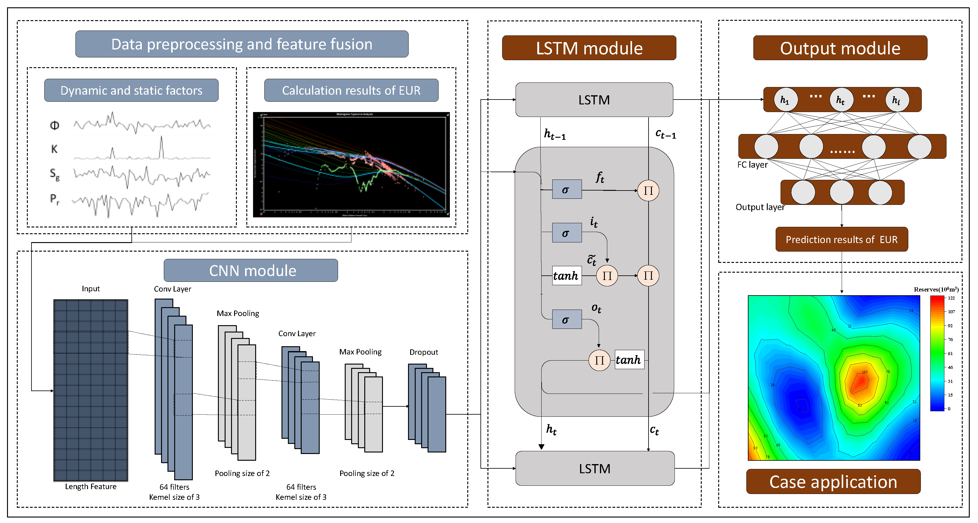
Figure 1. Flow Chart of Dynamic Reserve Prediction.
Symmetry 17 02033 g001
Figure 2. Convolutional Neural Network Structure Diagram.
Symmetry 17 02033 g002
Figure 3. The structural diagram of LSTM.
Symmetry 17 02033 g003
Figure 4. CNN-LSTM Structure Diagram.
Symmetry 17 02033 g004
Figure 5. Pearson correlation coefficient heatmap of dynamic and static parameters (the size of the circle area represents the strength of the linear relationship).
Symmetry 17 02033 g005
Figure 6. Comparison of different prediction models. (a) CNN; (b) LSTM; (c) CNN-LSTM.
Symmetry 17 02033 g006
Figure 7. Predicted versus Actual Dynamic Reserves.
Symmetry 17 02033 g007
Figure 8. Comparison between the predicted and measured dynamic reserves of adjacent multi-well groups.
Symmetry 17 02033 g008
Table 1. Dynamic and Static Influencing Parameters.
Parameter NameMinimum ValuesMaximum Values
Porosity/(%)4.2213.36
Penetration rate/(10−3 μm2)0.147.08
Gas saturation/(%)28.6369.00
Single-layer effective thickness/(m)1.908.20
Formation pressure/(MPa)5.2129.71
Pre-production set pressure/(MPa)22.0028.00
Daily gas production/(104 m3/d)0.195.97
Accumulated gas production/(104 m3)281.966984.73
Casing pressure/(MPa)1.0822.53
Oil pipe pressure/(MPa)0.555.94
Production time (a)112
Table 2. Evaluation Results of Different Prediction Models.
ModelR2MAERMSEMAPE
CNN0.68613.04318.3150.314
LSTM0.73113.22717.4720.332
CNN-LSTM0.9595.3117.6270.139
Table 3. The Results of Different Models.
ModelR2MAERMSEMAPE
decision tree0.73612.85616.9320.295
Support Vector Machine0.68614.21319.0470.324
linear regression0.78511.32815.6410.274
BP neural network0.82510.57414.2830.263
CNN-LSTM model0.9595.3117.6270.139
Disclaimer/Publisher’s Note: The statements, opinions and data contained in all publications are solely those of the individual author(s) and contributor(s) and not of MDPI and/or the editor(s). MDPI and/or the editor(s) disclaim responsibility for any injury to people or property resulting from any ideas, methods, instructions or products referred to in the content.