Graph-FEM/ML Framework for Inverse Load Identification in Thick-Walled Hyperelastic Pressure Vessels

Abstract

The accurate identification of internal and external pressures in thick-walled hyperelastic vessels is a challenging inverse problem with significant implications for structural health monitoring, biomedical devices, and soft robotics. Conventional analytical and numerical approaches address the forward problem effectively but offer limited means for recovering unknown load conditions from observable deformations. In this study, we introduce a Graph-FEM/ML framework that couples high-fidelity finite element simulations with machine learning models to infer normalized internal and external pressures from measurable boundary deformations. A dataset of 1386 valid samples was generated through Latin Hypercube Sampling of geometric and loading parameters and simulated using finite element analysis with a Neo-Hookean constitutive model. Two complementary neural architectures were explored: graph neural networks (GNNs), which operate directly on resampled and feature-enriched boundary data, and convolutional neural networks (CNNs), which process image-based representations of undeformed and deformed cross-sections. The GNN models consistently achieved low root-mean-square errors (≈0.021) and stable correlations across training, validation, and test sets, particularly when augmented with displacement and directional features. In contrast, CNN models exhibited limited predictive accuracy: quarter-section inputs regressed toward mean values, while full-ring and filled-section inputs improved after Bayesian optimization but remained inferior to GNNs, with higher RMSEs (0.023–0.030) and modest correlations (R2). To the best of our knowledge, this is the first work to combine boundary deformation observations with graph-based learning for inverse load identification in hyperelastic vessels. The results highlight the advantages of boundary-informed GNNs over CNNs and establish a reproducible dataset and methodology for future investigations. This framework represents an initial step toward a new direction in mechanics-informed machine learning, with the expectation that future research will refine and extend the approach to improve accuracy, robustness, and applicability in broader engineering and biomedical contexts.

1. Introduction

The mechanical integrity of thick-walled pressure vessels—especially those composed of hyperelastic materials—is pivotal across multiple engineering domains, from elastomeric seals and biomedical devices to soft robotics and energy storage systems. Unlike thin-walled vessels, where classical formulas provide sufficiently accurate stress and deformation predictions, thick-walled vessels exhibit complex nonlinear deformation behaviors under internal and external loading. Accurately estimating internal pressure loads in such systems is often critical; however, direct measurement inside the vessel is usually impractical, particularly when the vessels are opaque or inaccessible. Thus, inverse load identification—inferring boundary loads from observable deformations—emerges as a practical and non-invasive approach to structural health monitoring and reverse engineering.

1.1. Motivation and Problem Context

Hyperelastic materials, such as rubbers and bio-inspired polymers, exhibit large deformations and nonlinear stress–strain responses that defy linear elastic assumptions. Analytical and numerical treatments for thick-walled hyperelastic vessels—especially in cylindrical or spherical geometries—have advanced, utilizing models such as Neo-Hookean, Mooney–Rivlin, and Yeoh. For instance, [1] derived analytical solutions for stress and deformation under various loading conditions, validated with finite element simulations, thereby enhancing computational efficiency in design studies [1]. However, these methods typically focus on forward problems—predicting deformation given known pressure loads—not on the inverse scenario, where the goal is to deduce unknown loading conditions from deformation measurements.

In practical applications—such as pressure monitoring in subsurface pipelines or biomedical implants—only deformations at accessible boundaries are observable, often via imaging or surface sensors. Therefore, there is a compelling need for robust methodologies that can infer internal and external pressures from boundary deformation data. The potential utility of such inverse load identification methods is especially high when combined with machine learning (ML) techniques, capable of handling complex nonlinearities and large parameter spaces.

1.2. Existing Inverse Load Identification Strategies

Inverse load identification has traditionally been approached through gradient-based optimization, sensitivity analysis, or classical regression methods. For example, ref. [2] investigated distributed load identification on hyperelastic plates using displacement measurements. They evaluated techniques such as polynomial regression, support vector regression, and neural networks, combined with gradient-based sensitivity analyses, achieving accurate load estimates under certain conditions [2].

However, those methods have limitations when extended to thick-walled geometries or large-deformation regimes typical of hyperelastic materials. Particularly, they rely heavily on carefully tuned models and are prone to instability or overfitting when the input parameter space is vast or when data are noisy.

1.3. Emergence of Physics-Informed and Graph-Based Neural Networks

Scientific machine learning (SciML) has ushered in innovations such as physics-informed neural networks (PINNs), which integrate governing physical laws—usually in the form of partial differential equations (PDEs)—into neural network training. PINNs enable networks to respect fundamental constraints like equilibrium, compatibility, or constitutive behavior, thereby improving generalization and physical plausibility even with limited training data [3,4]. These have been applied to both forward and inverse problems across deformation, elasticity, and fluid mechanics [3,5].

Graph Neural Networks (GNNs) have emerged as another powerful class of architectures, especially suited for irregular domains and non-uniform spatial discretization that naturally arise in deforming structures. They operate on graph representations—nodes connected by edges—using message-passing mechanisms to capture spatial correlations. This is particularly beneficial for boundary deformation data, which do not conform neatly to uniform grids [6,7]. GNNs have demonstrated notable success in simulating PDE-constrained inverse problems—such as reconstructing initial conditions or material properties from sparse measurements—often outperforming traditional solvers in both accuracy and computational speed [7].

Parallel research has hybridized graph-based models with physics-informed formulations. Physics-informed Graph Neural Galerkin Networks, for example, incorporate PDE residuals into graph-based architectures for solving inverse and forward mechanics problems [8].

1.4. Research Gaps and Our Contributions

Despite these advances, no study—according to our literature review—has combined boundary deformation observations with GNN-based inverse frameworks for thick-walled hyperelastic vessels. Most efforts focus on plates, shells, or simpler geometries, or utilize forward-only prediction frameworks.

Therefore, this work introduces a novel Graph-FEM/ML framework designed to identify the normalized internal and external pressures ($p_i/C$, $p_o/C$) in thick-walled hyperelastic vessels, where $p_i$ and $p_o$ denote the internal and external pressures, respectively, and C represents the shear modulus of the material. The inputs to the network consist of the vessel boundaries—both inner and outer surfaces—in their undeformed and deformed configurations, ensuring that physically measurable quantities are directly exploited for inverse load identification.

Figure 1 illustrates the conceptual model of the uniform thick-walled hyperelastic pressure vessel considered in this study. The geometry is represented by a mid-ellipsoidal cross-section characterized by the semi-major axis $a$, the semi-minor axis $b$, and the uniform wall thickness $t$. The vessel is bounded by an inner boundary, which is subjected to the internal pressure $p_i$, and an outer boundary, which is exposed to the external pressure $p_o$. In the proposed framework, both the undeformed and deformed configurations of these boundaries are extracted and employed as input data for the machine learning models. This choice reflects realistic experimental conditions since boundary displacements can be measured non-invasively through imaging or sensing techniques. By correlating these measurable boundary deformations with the normalized pressure ratios ($p_i/C, p_o/C$), where $C$ denotes the shear modulus of the material, the framework enables inverse identification of the applied loading conditions in uniform thick-walled hyperelastic vessels.

Our framework features several key innovations:

• Dataset generation via automated FEM simulations: using Latin Hypercube Sampling (LHS) on the geometrical parameters ($a/b,t/b$)—where $a$, $b$, and $t$ denote the semi-mid major diameter, semi-mid minor diameter, and wall thickness of the vessel, respectively—to generate diverse deformed boundary datasets via ANSYS 2024R1 APDL scripting.
• Boundary representation through graphs: This allows dimensionality reduction and irregular sampling, consistent with real-world deformation measurements.
• Extraction of geometric cues: including displacement differences, normals, tangents, and curvature along boundaries, to enrich input features. Curvature was initially evaluated as part of the geometric feature set; however, subsequent analysis showed that its numerical sensitivity reduced feature consistency across samples. It was therefore considered in the early stages but ultimately excluded from the final model.
• GNN architectures enriched with Bayesian hyperparameter optimization, alongside comparisons against CNNs and baseline regressors (e.g., MLPs), to assess performance and robustness.
• Generalization across partial to full cross-sections: including ¼ and full ring geometries to evaluate coverage of deformation patterns.
• While several hybrid machine learning–mechanics frameworks have been proposed in recent years, including physics-informed neural networks (PINNs), reduced-order FEM surrogates, and symmetry-aware deep learning models, their applications have largely remained limited to forward or parameter-identification problems. In contrast, the present study addresses a distinct and previously untested scenario—the inverse identification of dual internal and external pressures in thick-walled hyperelastic vessels based solely on measurable boundary deformations.
• To the best of our knowledge, no prior work has exploited boundary deformation data represented as graph-structured inputs to infer pressure loads in nonlinear hyperelastic systems. This work therefore introduces the first boundary-informed Graph-FEM/ML framework that learns a direct inverse mapping from deformed boundaries to normalized pressure ratios. The proposed approach uniquely combines (i) high-fidelity FEM-based data generation, (ii) mechanics-informed geometric features (displacements, normals, and tangents), and (iii) graph neural network (GNN) architectures optimized via Bayesian search.
• By explicitly leveraging physically measurable boundary information and graph-based relational learning, this study establishes a new paradigm for non-invasive load identification in hyperelastic materials—bridging the gap between traditional inverse FEM optimization and modern graph-driven learning in computational mechanics.

1.5. Structure of the Paper

The remainder of this paper is organized as follows:

• Section 2 (Background and Related Work) situates our contribution within the broader literature on inverse load identification, ML–FEM integration, physics-informed methods, and GNNs in computational mechanics.
• Section 3 (Problem Statement and Governing Equations) formalizes the geometric and material modeling—including the use of a Neo-Hookean constitutive model, pressure normalization, and the definition of the inverse mapping from boundary deformations to pressure loads.
• Section 4 (Dataset Generation via FEM) details our parametrized design approach (via LHS) and execution of ANSYS simulations to amass a robust dataset for training.
• Section 5 (Data Preprocessing and Feature Engineering) outlines strategies to resample boundary data uniformly and extract enriched geometric features amenable to graph-based modeling.
• Section 6 (Machine Learning Framework) describes the ML architectures tested, training methods, and the use of Bayesian optimization in tuning hyperparameters.
• Section 7 (Results and Discussion) presents both quantitative performance metrics (e.g., RMSE, correlation coefficients) and qualitative visualizations, comparing models, input representations, and optimization strategies.
• Section 8 (Conclusions) recaps the contributions, acknowledges limitations, and points toward future extensions—such as adding noise robustness, experimenting with more complex material models (e.g., Ogden), or exploring axisymmetric and non-axisymmetric loading.

By integrating advanced ML approaches with robust boundary-informed FEM simulations, this study aims to fill a critical gap in inverse load identification for hyperelastic pressure vessels, offering a scalable pathway toward non-invasive structural sensing and diagnostics.

2. Background and Related Work

Inverse problems occupy a central role in mechanics, where the objective is often to infer hidden system states or parameters from observable quantities. In structural mechanics, one of the most challenging inverse problems is the identification of loads from measured displacements or deformations. Classical forward analyses predict displacements given known loads, while the inverse counterpart works in the opposite direction. Such problems are intrinsically ill-posed, sensitive to noise, and computationally demanding. Over the last two decades, progress in computational mechanics, optimization, and machine learning (ML) has opened promising new pathways for tackling these challenges.

This section provides a detailed overview of prior work across four themes that directly underpin this study: (i) inverse load identification in mechanics, (ii) hyperelastic material modeling in pressure vessels, (iii) finite element method (FEM) integration with ML, (iv) convolutional neural networks (CNNs) in computational mechanics, and (v) graph neural networks (GNNs) and their adoption in computational mechanics.

2.1. Inverse Load Identification in Structural and Continuum Mechanics

Load identification problems are classical in structural analysis. Early contributions relied on deterministic optimization strategies that minimized the difference between observed and computed displacements [9]. Sensitivity methods and adjoint formulations became popular in the 1990s and 2000s, enabling efficient computation of gradients for updating load parameters [10]. Despite their rigor, these methods struggled with highly nonlinear behaviors and noisy data.

Recent reviews highlight the continued relevance and evolving techniques in dynamic load identification. For example, ref. [11] summarized methods ranging from Kalman filters to regularized optimization and neural network strategies, stressing both progress and open challenges in handling real-world data.

For hyperelastic materials, inverse identification is even more complex. Ref. [2] demonstrated that distributed loads on hyperelastic plates could be recovered using regression methods, but their work also showed the sensitivity of results to dataset quality and feature selection. Their study indicates that although ML methods such as support vector regression and neural networks improve accuracy, they remain constrained by the representation of geometric nonlinearities and data scarcity.

The consensus across the literature is that inverse load identification remains an ill-posed and underdetermined problem, requiring sophisticated regularization, robust feature engineering, or the incorporation of physical knowledge to stabilize and generalize solutions.

2.2. Hyperelastic Materials and Thick-Walled Pressure Vessels

Hyperelastic materials exhibit finite strains under relatively small stresses, governed by strain energy density functions such as Neo-Hookean, Mooney–Rivlin, and Ogden models [12,13]. Their ubiquity in engineering—from automotive seals to biomedical implants—demands accurate computational models.

Analytical studies of thick-walled hyperelastic cylinders and spheres date back to Rivlin’s seminal works, with continued developments improving efficiency and expanding applicability. Ref. [1] provided analytical solutions for incompressible, isotropic, and hyperelastic thick-walled vessels under pressure loads, comparing them against FEM simulations. Their work demonstrated that analytical methods could cover a broad parameter range, but FEM remains indispensable when handling more complex geometries or boundary conditions.

In the context of inverse problems, thick-walled vessels are particularly relevant because boundary deformations are measurable in laboratory or field settings (e.g., via digital image correlation or ultrasound). Thus, they represent an ideal testbed for frameworks that attempt to identify loads from deformations. However, we found no studies that directly connect boundary deformations to pressure load estimation in hyperelastic vessels, confirming the novelty of our approach.

2.3. Finite Element Method (FEM) Coupled with Machine Learning

The finite element method (FEM) has long been the workhorse of computational mechanics, providing a flexible and robust framework for solving complex structural and continuum problems. In recent years, its integration with machine learning (ML) has gained significant momentum, largely motivated by two needs: first, to accelerate computationally expensive simulations, and second, to address inverse problems that involve large and high-dimensional datasets.

Several notable approaches illustrate this trend. Ref. [14] introduced a FEM-informed neural network that incorporates simulation outputs directly into the training process, enabling applications to both forward and inverse problems. Their results demonstrated that embedding FEM knowledge improves data efficiency and enhances the stability of network predictions. Other researchers have employed reduced-order modeling and surrogate approaches, often using autoencoders or regression techniques to approximate FEM solutions and provide rapid predictions of stress or displacement fields [15]. Building on this idea, ref. [15] also combined reduced-order modeling with graph neural networks (GNNs) to handle non-parametric geometries in structural dynamics, highlighting the scalability and versatility of hybrid ML–FEM strategies.

Collectively, these studies emphasize a broader trend in the field: machine learning is not intended to replace FEM, but rather to complement it. In most cases, ML either serves as a surrogate model to reduce the cost of repeated FEM simulations or as a mechanism to embed FEM-derived knowledge into the learning process, thereby bridging numerical accuracy with data-driven efficiency.

2.4. Graph Neural Networks in Computational Mechanics

Graph neural networks (GNNs) are designed to process non-Euclidean data, which makes them particularly well-suited for the irregular meshes and point clouds commonly encountered in computational mechanics. Unlike convolutional neural networks (CNNs), which rely on grid-like structures, GNNs exchange information through message passing between nodes and edges, enabling a natural representation of finite element meshes and discretized structural boundaries. This capability is especially advantageous in mechanics problems where geometry and topology are highly irregular.

Recent studies have demonstrated the versatility of GNNs across a wide range of applications. For instance, ref. [6] applied GNNs to partial differential equation (PDE)-constrained inverse problems, showing that they can efficiently solve high-dimensional systems. In the field of structural dynamics, ref. [16] developed an adaptive mesh-based GNN framework capable of simulating displacement fields and crack propagation in phase-field fracture models. Similarly, ref. [15] combined reduced-order modeling (ROM) with GNNs to address non-parametric geometries in structural dynamics, striking a balance between computational efficiency and physical fidelity. Complementing these developments, ref. [17] employed GNNs within the deep energy method, where the graph-based formulation was directly linked to FEM shape functions for gradient computation.

Comprehensive reviews [7,18] underline that GNNs are emerging as a powerful alternative to CNNs in computational mechanics, especially for problems defined on irregular domains where graph-based representation is both natural and efficient. These characteristics position GNNs as a key component of modern mechanics-informed machine learning frameworks, including the Graph-FEM/ML approach proposed in this study.

Recent advances demonstrate hybrid approaches for inverse solid-mechanics problems. For example, ref. [19] developed a Neural-Integrated Meshfree method for finite-strain hyperelasticity. Authors of ref. [8] proposed a Physics-informed Graph Neural Galerkin network to handle forward/inverse PDEs on unstructured meshes. The authors in ref. [20] reviewed the fusion of PINNs and GNNs for inverse analyses in complex geometries.

Despite these developments, none of them exploit boundary-deformation graphs in combination with hyperelastic dual-pressure vessels as formulated in this study.

2.5. Convolutional Neural Networks (CNNs) in Computational Mechanics

Convolutional neural networks (CNNs) have become increasingly important in computational mechanics due to their ability to automatically extract hierarchical spatial features from structured data. Originally developed for image recognition [21,22], CNNs have been adapted to mechanics problems where domains or simulation outputs can be represented as images or voxel grids.

CNNs have been widely applied as surrogate models to accelerate FEM analyses. For instance, ref. [23] predicted stress fields in heterogeneous materials, while [24] used CNNs for fluid–structure interactions. They have also been employed in inverse analyses, such as material parameter identification [25] and defect detection in structural health monitoring [26]. The convolution operation’s translation-invariance is particularly effective for capturing repeated patterns in stress and strain fields.

A key limitation of CNNs is their reliance on regular grids, which can be inefficient for curved or irregular geometries common in mechanics. Although image-based discretizations are possible, they may introduce resolution artifacts. To overcome this, recent research explores hybrid approaches, combining CNNs with FEM or physics-informed constraints [27,28].

In summary, CNNs are well-suited for computational mechanics tasks where structured representations are available, such as vessel cross-sections used in this study. However, their limitations on irregular domains highlight the complementary role of graph-based models, motivating the combined Graph-FEM/ML approach developed here.

2.6. Research Gap and Positioning of This Work

From the synthesis of the literature, several key insights can be drawn. Inverse load identification has received limited attention in the context of thick-walled hyperelastic vessels, with most existing studies focusing instead on plates, shells, or thin-walled geometries. Although finite element studies on hyperelastic materials have provided valuable analytical and numerical insights, they have not yet addressed the direct inference of applied loads from boundary deformations. While hybrid approaches combining FEM and machine learning have proven effective, these have primarily been employed as forward surrogates to accelerate simulations rather than as inverse models for load recovery. Graph neural networks (GNNs) offer strong capabilities for handling irregular boundaries and meshes, yet their use in mechanics is still recent, with very limited studies addressing load identification tasks. Convolutional neural networks (CNNs) have demonstrated strong potential in learning spatial patterns from structured data, yet their application in mechanics remains largely focused on surrogate modeling and material characterization, with relatively few studies addressing inverse load identification in complex structural systems.

This study aims to fill these gaps by introducing a Graph-FEM/ML framework in which measurable boundary deformations are represented as graph inputs to neural networks trained to predict normalized internal and external pressure loads. By combining FEM-based simulation for dataset generation, geometric feature engineering for enriched input representations, and advanced machine learning architectures including CNNs, GNNs, and Bayesian optimization, this work establishes a novel and comprehensive approach to inverse load identification in thick-walled hyperelastic pressure vessels.

To further clarify the positioning of this study within the broader context of inverse modeling in mechanics,

Table 1. Comparative summary of major inverse modeling approaches in computational mechanics.

Approach	Typical Input Data	Physics Incorporation	Geometric Flexibility	Learning Paradigm	Common Limitations	Relevance to This Work
Classical Inverse FEM/Adjoint Methods	Displacements or stresses at selected nodes	Full governing equations (explicit)	Limited (requires consistent mesh)	Deterministic optimization	Sensitive to noise; high computational cost	Basis for benchmark; lacks data efficiency
Regularized Least Squares/Sensitivity-based Inversion	Displacement or strain measurements	Partial; depends on sensitivity matrices	Moderate	Regression with manual regularization	Requires tuning; unstable for nonlinear materials	Conceptually related but not scalable
Physics-Informed Neural Networks (PINNs)	Pointwise field data (stress/strain)	Implicit (via PDE residuals)	High (mesh-free)	Continuous field learning	Slow convergence for stiff PDEs; less effective on boundaries	Shares physics-driven idea but not boundary-focused
CNN-based Surrogates	Image-like FEM fields or cross-sections	Weak (data-only)	Moderate (grid-based)	Spatial convolutional learning	Grid artifacts; limited for irregular shapes	Used here for baseline comparison
Proposed Graph-FEM/ML (This Study)	Boundary deformations (undeformed + deformed)	Implicitly preserved via FEM-generated data	High (graph-based irregular domains)	Relational learning via GNNs	Currently limited to Neo-Hookean materials; noise-free data	Introduces boundary-informed GNN inversion for hyperelastic vessels

The table shows that while PINNs and classical inverse FEM exploit physics explicitly, they often require full-field data or complex adjoint derivations. CNNs can process structured images but struggle with curved or irregular geometries. The proposed boundary-informed Graph-FEM/ML framework complements these approaches by directly learning from graph-encoded boundary displacements—a representation that is both physically measurable and computationally efficient for inverse pressure identification in nonlinear hyperelastic systems.

summarizes representative approaches and their key characteristics. The comparison highlights how the proposed Graph-FEM/ML framework bridges the gap between physics-based inverse FEM optimization and data-driven learning methods by exploiting measurable boundary information in a graph-structured form.

3. Problem Statement and Governing Equations

The problem studied in this work concerns the inverse identification of internal and external pressures in a uniform thick-walled hyperelastic vessel based on measurable boundary deformations. The vessel is modeled with an ellipsoidal cross-section defined by the major diameter a, the minor diameter b, and the uniform wall thickness t. The material is assumed isotropic, incompressible, and hyperelastic, represented by the Neo-Hookean strain energy function.

3.1. Governing Equations for Hyperelastic Vessels

The starting point for modeling the mechanical response of thick-walled hyperelastic vessels is the choice of a suitable constitutive relation. Hyperelastic materials are distinguished by their ability to undergo very large, reversible deformations while maintaining a nonlinear relationship between stress and strain. Such materials include elastomers, rubber-like polymers, and biological tissues such as arteries [12,29]. Unlike linear elastic solids, whose stress–strain relationship is characterized by a constant stiffness, hyperelastic materials are described by a strain energy density function, which defines the stored elastic energy per unit volume as a function of strain invariants or principal stretches. Once strain energy density function is specified, the corresponding stress tensors can be systematically derived.

For an incompressible, isotropic hyperelastic material, the strain energy function can be expressed in terms of the invariants of the right or left Cauchy–Green deformation tensors. Among the available models, the incompressible neo-Hookean model with the shear modulus $C$ of the material represents one of the simplest, yet most widely used forms. This material model is especially relevant for thick-walled vessels under internal and external pressures. It is particularly effective in capturing moderate to large deformations in elastomers and polymeric materials, and it forms the baseline for more advanced models such as Mooney–Rivlin or Ogden [13,30].

In such problems, the vessel walls experience combined radial and circumferential (hoop) stretching, often accompanied by finite axial strains depending on the boundary conditions. For spherical or cylindrical vessels, analytical solutions for radial and hoop stresses have been derived [30,31]. For ellipsoidal vessels with arbitrary aspect ratios $a/b$, however, closed-form solutions are generally not available, and numerical methods such as the finite element method (FEM) are required to compute the stress and displacement fields.

A key characteristic of the Neo-Hookean model is its ability to represent nonlinear stiffening behavior with increasing deformation. For small strains, the model reduces to a linear elastic relationship where the shear modulus $C$ is proportional to the initial slope of the stress–strain curve. At larger deformations, the quadratic dependence on stretches ensures that stresses rise more sharply, capturing the strain-hardening effects typical of rubbers. This makes the model both physically relevant and mathematically convenient for simulating large deformation in pressure vessels.

From the perspective of inverse load identification, the importance of these governing equations lies in the mapping between boundary deformations and applied loads. The Neo-Hookean formulation ensures that stresses and displacements are uniquely linked through well-established continuum mechanics relations. Consequently, any machine learning model trained to approximate the inverse mapping

$$f^{-1}:\Delta {\mathit{u}}_{\mathit{b}\mathit{o}\mathit{u}\mathit{n}\mathit{d}\mathit{a}\mathit{r}\mathit{y}}\to (p_i/C,p_o/C)$$

implicitly inherits this physics-based relationship. The FEM-generated data used for training embodies these constitutive and equilibrium conditions, ensuring that the machine learning framework does not learn arbitrary correlations but rather approximates a physically consistent inverse operator.

3.2. Summary of Problem Statement

In conclusion, the problem investigated in this work involves a uniform thick-walled hyperelastic vessel with an ellipsoidal cross-section modeled using an incompressible neo-Hookean constitutive law. The vessel is subjected to internal and external pressures, which are normalized by the shear modulus of the material to yield dimensionless load parameters. The forward problem consists of solving the equilibrium equations and constitutive relations to predict boundary deformations under specified pressures, a task accomplished through finite element simulations due to the complexity of ellipsoidal geometries. The inverse problem, by contrast, requires predicting the normalized pressures from observed boundary deformations. This mapping is nonlinear and ill-posed, which motivates the use of a hybrid Graph-FEM/ML framework capable of learning the inverse operator from physically consistent simulation data. By defining the governing equations and constraints, this section establishes the physical and mathematical foundation upon which the proposed machine learning strategy is constructed.

4. Dataset Generation via FEM

A critical component of the proposed Graph-FEM/ML framework is the construction of a reliable and representative dataset that captures the nonlinear deformation behavior of thick-walled hyperelastic vessels under varying geometric and loading conditions. Since experimental datasets for such systems are extremely limited and often difficult to obtain, the dataset for this work was generated through systematic finite element simulations (FEM) using ANSYS 2024R1 Mechanical APDL scripting. This approach enables the exploration of a broad parameter space while maintaining full control over material properties, boundary conditions, and loadings.

4.1. Design Parameters

The geometry of the vessel is parameterized in terms of the aspect ratio and the relative wall thickness:

$$a/b, t/b$$

(1)

where $a$ and $b$ represent the semi-major and semi-minor axes of the mid-boundary ellipse, respectively (i.e., the semi-major and minor diameters of the mid-boundary, as illustrated in Figure 1), and $t$ denotes the uniform wall thickness of the vessel. In this study, $b$ is fixed as a known constant value. By varying the ratio $a/b$, the dataset spans a wide range of shapes, including oblate ellipsoids ($a/b>1$), prolate ellipsoids ($a/b<1$), and the special case of spherical geometry ($a/b=1$). The relative thickness $t/b$ ensures that both thin-walled and thick-walled configurations are represented in the dataset, covering the transition from shell-like to bulk material behavior.

In addition to geometry, the loading conditions are described in terms of dimensionless pressures, normalized with respect to the shear modulus $C$ of the neo-Hookean material:

$$p_i/C, p_o/C$$

(2)

where $p_i$ is the internal pressure and po is the external pressure. Normalization by $C$ eliminates material-scale dependence, allowing the dataset to capture purely geometric and loading effects in a dimensionless form.

4.2. Sampling Strategy

To ensure statistically uniform coverage of the multi-dimensional parameter space, Latin Hypercube Sampling (LHS) was employed [32]. LHS is a stratified sampling technique that partitions the range of each variable into equally probable intervals and ensures that the full range of each factor is explored without redundancy. Compared to simple random sampling, LHS provides better space-filling properties and reduces the risk of clustering in certain regions of the parameter space, which is especially important for training machine learning models.

In this study, four factors were considered:

• Aspect ratio ($a/b$)
• Thickness ratio ($t/b$)
• Normalized internal pressure ($p_i/C$)
• Normalized external pressure ($p_o/C$)

The MATLAB R2024b script was used to generate the LHS matrix. The code specifies ranges for each parameter:

• $a/b$ in [0.5, 2.5]

• $t/b$ in [0.06, 0.5]

• $p_i/C$ in [0.0, 0.1]

• $p_o/C$ in [0.0, 0.1]

Fifty initial design points were generated for demonstration in the uploaded script, but in the final campaign a larger set was created to ensure coverage. The generated samples were automatically categorized into ellipsoid types (oblate, prolate, or sphere) and assigned a thickness parameter that combines geometric ratios to reflect effective slenderness of the vessel. The outputs were stored in a design-of-experiments (DOE) table and exported as a CSV file to serve as input for the FEM batch simulations.

To clarify the geometric limits of the sampled vessels, the actual constants used in the simulation were $b = 100 \mathrm{m}\mathrm{m}$ and $C = 0.5 \mathrm{M}\mathrm{P}\mathrm{a}$. Based on the prescribed sampling ranges ($a/b \in [0.5, 2.5], t/b \in [0.06, 0.5]$), the minimum and maximum semi-axes of the ellipsoidal vessels are summarized in

Table 2. Minimum and maximum semi-axes of ellipsoidal vessels based on sampling ranges (b = 100 mm).

Parameter	Minimum (mm)	Maximum (mm)	Notes
Mid-surface semi-major axis ($a$)	50	250	From $a/b = 0.5 \to 2.5$
Inner semi-major axis ($a - t/2$)	0	244	Depends on thickness ratio
Outer semi-major axis ($a + t/2$)	56	256	Depends on thickness ratio
Mid-surface semi-minor axis ($b$)	100	100	Constant $b = 100 \mathrm{m}\mathrm{m}$
Inner semi-minor axis ($b - t/2$)	75	97	Depends on thickness ratio
Outer semi-minor axis ($b + t/2$)	103	125	Depends on thickness ratio

. The results highlight the geometric diversity of the dataset and provide a clear sense of the scale of the generated samples.

This table highlights that the generated dataset spans a broad range of geometries, from nearly spherical configurations ($a/b\approx 1$) to strongly oblate or prolate shapes ($a/b<1 or a/b>1$), and from thin walled to very thick-walled vessels ($t/b=0.06\to 0.5$). The extreme lower bounds, where the inner semi-axes of the vessel approach zero, correspond to unrealistic cases that typically cause FEM convergence failures. Such degenerate geometries were excluded, resulting in a final dataset of 1386 valid samples that provide a robust basis for the subsequent machine learning analysis.

To ensure reproducibility and consistency across all finite element analyses, the FEM setup used to generate the deformation dataset was implemented via a parameterized APDL script under an axisymmetric formulation in the R–Z plane. The ellipsoidal vessel was modeled as a thick-walled, nearly incompressible neo-Hookean material subjected to uniform internal and external pressures. The principal modeling parameters are summarized in

Table 3. Summary of FEM modeling parameters for the axisymmetric ellipsoidal vessel.

Category	Setting/Description
Analysis type	2D axisymmetric large-deformation (NLGEOM, ON)
Element type	8-node quadratic PLANE182, axisymmetric option (KEYOPT(1,3) = 1)
Material model	Neo-Hookean hyperelastic, $C_{10}=0.5 \mathrm{M}\mathrm{P}\mathrm{a}$, $D_1=1\times {10}^{-4}\hspace{0.17em}\mathrm{M}\mathrm{P}{\mathrm{a}}^{-1}$
Geometry	Ellipsoidal cross-section: $a_{mid}=100 \mathrm{m}\mathrm{m},b_{mid}=50 \mathrm{m}\mathrm{m},t=20 \mathrm{m}\mathrm{m}$
Mesh	Mapped quadrilateral mesh, element size $\approx t/30$; element aspect ratio < 2
Boundary conditions	Axis line $R=0$: $UX=0$; Equator $Z=0$$: UY=0$(mirror symmetry)
Loading	Uniform internal/external pressures; default $p\_in=0.1 \mathrm{M}\mathrm{P}\mathrm{a}$, $p_{out}=0$
Solution control	Automatic time stepping (AUTOTS, ON); NSUBST (50, 100, 20); force/displacement tolerance ≈ 1%
Output data	Nodal coordinates (undeformed and deformed), UX, UY, USUM; exported for ML preprocessing

This axisymmetric representation captures the full three-dimensional deformation response with high computational efficiency. The spline-based smooth boundaries, mapped meshing, and uniform element sizing guarantee numerical stability and geometric fidelity. The exported nodal displacements along the inner and outer walls form the physically consistent boundary dataset employed in the subsequent Graph-FEM/ML analysis.

.

4.3. FEM Simulations

For each design point generated by the LHS procedure, an FEM model was built and solved in ANSYS Mechanical APDL. The Neo-Hookean constitutive model was implemented, and large-deformation analysis was activated to capture nonlinear kinematics. Internal and external pressures corresponding to the sampled values ($p_i/C,p_o/C$) were applied as surface tractions on the inner and outer boundaries, respectively.

The FEM analysis produced displacement fields for the vessel walls, from which the inner and outer boundary curves were extracted both in undeformed and deformed configurations. These boundary datasets constitute the primary inputs to the machine learning framework.

As an illustrative example, Figure 2 and Figure 3 present typical FEM outputs for a vessel geometry defined by semi-major axis $a_{mid}=100\hspace{0.17em}\mathrm{m}\mathrm{m}$, semi-minor axis $b_{mid}=50\hspace{0.17em}\mathrm{m}\mathrm{m}$, and thickness $t=20\hspace{0.17em}\mathrm{m}\mathrm{m}$. The material was modeled as Neo-Hookean with parameters $C=0.5\hspace{0.17em}\mathrm{M}\mathrm{P}\mathrm{a}$ and $D=1\times {10}^{-4}\hspace{0.17em}\mathrm{M}\mathrm{P}{\mathrm{a}}^{-1}$. The model was subjected to an internal pressure of $0.1\hspace{0.17em}MPa$ and zero external pressure.

Out of the total 2000 design points generated via LHS, a subset of 1386 samples successfully converged in FEM analysis and produced valid deformation data. The remaining cases failed due to extreme geometric slenderness or load combinations that led to numerical instability, which is common in large deformation hyperelastic simulations. The final dataset of 1386 samples therefore forms the basis for training, validation, and testing of the neural network models.

To confirm the numerical stability of the finite element analyses, a mesh convergence test was performed on the baseline model (a_mid = 100 mm, b_mid = 50 mm, t = 20 mm) using the Neo-Hookean material formulation under an internal pressure of 0.1 MPa. The convergence history of the nonlinear solver is illustrated in Figure 4, showing the evolution of the absolute convergence norms (force and displacement) over successive cumulative iterations. The rapid decay of both force and displacement residuals within the first few iterations and their subsequent stabilization below 10⁻² confirm the satisfactory convergence of the solution. These results demonstrate that the FEM setup and mesh density used in this study provide numerically consistent and mesh-independent deformation results, ensuring the reliability of the dataset employed for machine learning.

4.4. Rationale for Boundary Data

A crucial methodological choice in this work is the use of boundary deformations as the sole input data for the inverse identification problem. The justification is twofold.

First, from a practical standpoint, boundary displacements represent quantities that are experimentally measurable using techniques such as digital image correlation (DIC), ultrasound imaging, or laser scanning. Unlike internal stress fields, which are inaccessible without intrusive instrumentation, boundary deformations can be monitored non-invasively in laboratory or in-service conditions.

Second, from a theoretical standpoint, boundary data carry sufficient information to encode the effects of internal and external pressures. According to continuum mechanics principles, stresses and strains within the material must equilibrate with the boundary tractions. Thus, changes in applied pressures inevitably manifest as measurable boundary displacements. By training the ML model to link boundary displacements directly to normalized pressures, the proposed framework exploits physically consistent and practically relevant data.

Moreover, to account for variations in boundary point density across different geometries, the boundary datasets were resampled to a uniform number of points per sample. This preprocessing step ensures that all FEM outputs are compatible in dimensionality, enabling consistent training of the neural networks. Additional geometric features such as displacement differences, normal and tangent vectors, and boundary curvature were also extracted in later stages to enrich the input representation.

4.5. Summary

In summary, the dataset generation process integrates design-of-experiments techniques with finite element simulations to produce a comprehensive and physically grounded dataset. The geometrical and loading parameters were systematically varied using Latin Hypercube Sampling across realistic ranges of aspect ratio, wall thickness, and normalized pressures. Finite element analyses of the sampled designs yielded boundary displacement data, which were extracted as undeformed and deformed inner and outer curves. A total of 1386 valid samples were retained for training and testing the proposed Graph-FEM/ML framework. The exclusive use of boundary data as model inputs is motivated by both practical measurability and theoretical sufficiency, thereby ensuring that the developed framework remains both scientifically rigorous and experimentally relevant.

5. Data Preprocessing and Feature Engineering

The dataset produced by the Latin Hypercube Sampling (LHS) design and subsequent finite element simulations in ANSYS 2024R1 Mechanical consisted of 1386 successful samples. Each of these samples is tagged with its corresponding normalized pressures ($p_i/C,p_o/C$) and is associated with the extracted inner and outer vessel boundaries in both undeformed and deformed states. At this stage, the challenge is to prepare these raw data for use as inputs to machine learning models, while ensuring compatibility with both graph-based neural networks (GNNs) and convolutional neural networks (CNNs).

The preprocessing and feature engineering procedures were structured in several stages, each targeting specific network architectures and enriched input representations.

5.1. Boundary Extraction and Resampling

The first step involved the systematic extraction of the inner and outer boundaries of the vessel cross-sections from the FEM simulations, for both undeformed and deformed states. Since each FEM simulation produced boundary discretizations with variable numbers of points, direct comparison across samples was not possible.

To achieve consistency across all FEM-generated samples, a boundary resampling strategy was employed. Specifically, the number of boundary points in each sample was uniformly reduced to match the smallest available node count among all simulations—which was consistently 241 points. This fixed value of 241 nodes per boundary (applied to inner and outer contours, in both undeformed and deformed states) ensured that every sample shared an identical dimensional structure without requiring any interpolation or artificial point generation. By enforcing this uniform 241-point representation, the physical fidelity of the FEM output was preserved, numerical artifacts were avoided, and the resulting dataset became fully compatible with graph-based learning architectures.

Resampled boundary points served as the direct input for the graph-based neural network, where each boundary point was treated as a node in the graph and connectivity was defined based on the ordering of points along the boundary.

5.2. Feature Augmentation: Displacements, Normals and Tangents

Beyond the raw boundary coordinates, additional geometric and kinematic features were derived to enrich the input representation. These features capture higher-order structural information that is potentially more informative for the inverse mapping:

• Boundary displacement differences (Δu):

For each boundary point, the displacement vector

$$\mathsf{\Delta }u=\left(x_{deformed}-x_{undeformed},y_{deformed}-y_{undeformed}\right)$$

(3)

was computed. This feature directly encodes the measurable deformation field from the FEM simulations. Light smoothing and z-score clipping were applied to mitigate outlier effects.

• Normal vectors:

Unit normals were computed for each boundary point in both undeformed and deformed configurations. Normals capture the outward direction of the wall surface and encode geometric changes induced by pressure loading.

• Tangent vectors:

Unit tangents were derived from the ordered boundary points. Tangents provide directional information along the vessel contour and complement the normal vectors by describing the local boundary orientation.

In this study, curvature values were not included in the final feature set. Although curvature was initially considered as a potential geometric descriptor, preliminary evaluations showed that the combination of displacement vectors with normal and tangent directions already provided sufficient discriminatory power while keeping the feature dimensionality compact. More detailed analysis across multiple FEM samples further revealed that κ is highly sensitive to small numerical fluctuations along the boundaries—particularly on the inner wall and in the deformed configuration. These fluctuations resulted in non-smooth curvature profiles that reduced feature consistency across samples and negatively affected the stability and generalization of the GNN training. For this reason, curvature was deliberately excluded, as it did not enhance predictive accuracy and in some cases degraded overall model robustness.

These features—Δu, normals, tangents, together with the raw boundary coordinates—were concatenated to form enriched node attributes. The resulting representation is well-suited for graph-based learning, where message-passing operations in graph neural networks can exploit both the geometric relationships and the deformation characteristics of the vessel boundaries.

5.3. CNN-Oriented Representations: Closed Cross-Sections

While GNNs excel at processing boundary data, CNNs require structured, image-like representations. To adapt the FEM output for CNN architectures, the extracted cross-sections were converted into binary or grayscale images where the vessel domain was represented as filled or hollow regions. Several configurations were created to explore CNN performance under different representations:

• Quarter cross-sections (¼ section): capturing local geometry with symmetry constraints.
• Full closed rings: representing the entire vessel in a single input image.
• Filled cross-sections: extending the representation to include fully filled vessel domains rather than hollow shells.

This dual approach (boundary graphs vs. image-based CNN inputs) allowed systematic comparison between architectures in terms of accuracy, generalization, and robustness.

5.4. Visualization Placeholders

Each of the preprocessing pipelines was supported with conceptual and numerical visualizations. For example:

• Boundary resampling: plots comparing original irregular boundary nodes with resampled uniform nodes.
• Feature augmentation: vector field illustrations of normals and tangents on deformed boundaries.
• CNN representations: side-by-side images of ¼, and full vessel sections in both hollow and filled form.

These figures will be positioned in the article to provide visual evidence of the preprocessing steps and highlight the distinction between graph-based and CNN-based approaches.

5.5. Summary Tables

To summarize the preprocessing strategies, two tables are provided below (

Table 4. Boundary-based features for graph neural networks.

Feature Type	Description	Role in GNN Training
Resampled boundary points	241 nodes uniformly per boundary	Graph node coordinates
Displacement differences	Δu between undeformed and deformed states	Encodes deformation field
Thickness variation	Distance between inner and outer walls	Captures wall response
Normal vectors	Outward unit vectors at each node	Orientation-sensitive feature
Tangent vectors	Unit tangents along boundaries	Local directional context

and

Table 5. Cross-sectional representations for convolutional neural networks.

Representation Type	Description	Purpose
Quarter section	¼ of vessel cross-section (hollow)	Symmetry-aware reduced domain
Full ring	Complete hollow cross-section	Global structural context
Filled quarter/half/full	Filled domains (not hollow)	Feature-rich images for CNNs

).

As illustrative examples of the preprocessing pipeline for the graph-based models, Figure 5, Figure 6, Figure 7 and Figure 8 present the boundary-derived features for Sample #1473. Figure 5 shows the raw undeformed and deformed boundary curves obtained from the FEM simulations, which serve as the baseline coordinate inputs to the neural network framework. In Figure 6, the effect of uniform subsampling is demonstrated, where the dense raw boundary points are reduced to a smaller set while still preserving the overall geometric fidelity of the contours; this step ensures consistent dimensionality and computational efficiency for the learning process. Figure 7 highlights the enriched geometric features extracted from the same sample: in the undeformed configuration, boundary points (U points) are plotted together with their associated unit normals ($n_U$, green), unit tangents ($t_U$, magenta), and displacement vectors (Δu, black) that directly link each undeformed node to its corresponding deformed position. These displacement vectors explicitly quantify both the magnitude and direction of local deformation. In the deformed configuration, the boundary points (D points) are displayed alongside their corresponding unit normals ($n_D$, green) and unit tangents ($t_D$, magenta). Finally, Figure 8 provides a magnified view of a selected region from Figure 6, allowing clearer visualization of the local geometric features and displacement vectors. This enlarged panel highlights the fine-scale directional differences and deformation patterns that may not be easily discernible in the full-boundary view. Taken together, these figures illustrate how raw boundary coordinates are progressively transformed into enriched node attributes that integrate displacement and directional information, thereby enhancing the representation used for graph-based neural network training.

In parallel with these GNN-oriented visualizations, a complementary set of figures will be provided for the convolutional neural network (CNN) representations. These will include quarter- and full-section cross-sectional images of the vessel, both in hollow and filled forms, to demonstrate how spatial patterns in the geometry and deformation field are encoded for CNN-based learning. This ensures a consistent and transparent comparison between the graph-based and image-based preprocessing strategies.

As illustrative examples of these CNN-oriented representations,

Table 6. CNN-oriented image representations of the vessel cross-section used for network input. Columns correspond to different preprocessing strategies (quarter section, full hollow ring, and full filled ring), while rows distinguish the undeformed (top) and deformed (bottom) states. This tabular layout highlights how boundary displacements and global shape changes are encoded for convolutional learning.

State/Configuration	Quarter Section (Local View)	Full Hollow Ring	Full Filled Ring
Undeformed (baseline)
Deformed (loaded)

depicts quarter- and full-section views of the vessel cross-section in both undeformed and deformed configurations. In the left column, quarter segments highlight local deformation features with reduced symmetry, while the central and right columns present the complete vessel as hollow and filled rings, respectively. The undeformed boundaries (blue, top row) and the deformed counterparts (red, bottom row) are shown side by side, clearly emphasizing outward displacements and changes in curvature induced by internal pressurization. By constructing both hollow and solid image variants, the preprocessing ensures that convolutional networks can extract not only contour-based information but also global shape changes across the entire domain. These CNN-oriented visualizations therefore provide a complementary modality to the graph-based inputs, enabling the networks to capture deformation-sensitive features at multiple spatial scales.

5.6. Concluding Remarks

Data preprocessing and feature engineering represent a cornerstone of the proposed framework. The dual-track approach, where resampled and enriched boundaries are exploited for GNNs and structured cross-sectional images are exploited for CNNs, ensures that the inverse load identification problem is tackled from complementary perspectives. The careful extraction of physically meaningful features—such as displacement differences, normals, and tangents—enables the networks to exploit not just raw geometric data but also higher-order mechanics-informed quantities. This multimodal preprocessing is expected to significantly enhance the generalization capacity and robustness of the trained models.

6. Machine Learning Framework

The success of data-driven modeling in computational mechanics and material systems critically depends on the choice of the machine learning framework. Building upon the boundary-derived features and enriched representations introduced in the previous sections, this study employs a range of neural architectures that have shown strong potential for capturing nonlinear mappings in high-dimensional scientific data. The recent literature demonstrates that convolutional neural networks (CNNs) are particularly effective for image-like structural representations, whereas graph neural networks (GNNs) are well suited for irregular boundary data and message-passing over node attributes [33,34]. Multi-layer perceptrons (MLPs), despite their relatively simple structure, remain a strong baseline for tabular or low-dimensional representations [35]. More recently, transformer-based architectures have been explored for mechanics-informed learning tasks, benefiting from self-attention mechanisms that capture long-range dependencies across nodes or pixels [36].

In this study, two complementary network types are selected as the core learning engines: graph neural networks (GNNs) and convolutional neural networks (CNNs). The choice is motivated by both the structure of the data generated through FEM simulations and the nature of the prediction task. On the one hand, boundary-derived datasets consist of irregular point clouds representing undeformed and deformed vessel contours. These data do not naturally reside on a regular grid but instead form sequences of nodes connected by geometric relationships. GNNs provide a natural framework for such irregular domains, as they operate directly on graph-structured data and propagate information through message passing between neighboring nodes [33,34]. By leveraging node attributes such as displacement vectors, normals, tangents, and curvature, GNNs can learn deformation-sensitive features that are inherently relational and spatially localized. This makes them particularly well-suited for capturing how local geometric changes accumulate into global structural responses.

On the other hand, CNNs remain indispensable for their proven capacity to handle structured image-based representations. The same FEM results can be rendered into cross-sectional images (e.g., hollow rings or filled sections), which allow CNNs to extract multi-scale spatial features in a translation-invariant manner [37,38]. These representations are especially valuable for capturing global deformation patterns and pressure-induced shape changes across the entire vessel wall. CNNs also benefit from decades of architectural advances and efficient GPU implementations, making them a strong complement to graph-based approaches.

The dual use of GNNs and CNNs thus provides a balanced modeling strategy: GNNs exploit the irregular, graph-like structure of boundary nodes, while CNNs capture image-like global patterns from rendered cross-sections. Together, they enable a comprehensive exploration of data representations for the inverse problem of mapping deformed shapes back to loading conditions, ensuring robustness and cross-validation of the learned models across different input modalities.

To ensure robust performance across these network types, Bayesian optimization is adopted for hyperparameter tuning, as it has been widely recognized for balancing exploration and exploitation in complex search spaces [39,40]. The entire framework is implemented in MATLAB with GPU acceleration, enabling scalable training over thousands of FEM-generated samples.

This section is therefore divided into two main parts. Section 6.1 provides an overview of the network architectures considered in this study, including CNN, GNN, MLP, and transformer models, and discusses their relevance to the boundary-feature learning task. Section 6.2 describes the training pipeline, the use of Bayesian optimization for hyperparameter selection, and the details of the software implementation. Together, these subsections provide a comprehensive description of the machine learning framework underpinning the proposed methodology.

6.1. GNNs and CNNs

6.1.1. Graph Neural Networks (GNNs)

Graph neural networks (GNNs) provide a natural framework for learning from data that are irregular, relational, and non-Euclidean in nature [33,34]. Unlike convolutional networks, which assume data lie on regular grids, GNNs operate directly on graph-structured representations where nodes contain features and edges encode spatial or physical relationships. This makes them particularly attractive for computational mechanics problems where mesh-based or boundary-based data dominate.

In the present study, the FEM simulations provide boundary curves in both undeformed and deformed configurations. These curves consist of sequentially connected nodes carrying attributes such as displacement differences (Δu), local thickness variation, unit normals, tangents, and curvature. Such attributes are inherently relational, since the meaning of each node is defined not only by its own features but also by its neighborhood along the boundary. By employing message passing, GNNs propagate and aggregate node features across edges, thereby learning how local deformations accumulate into global vessel responses. This capacity to respect irregular sampling, varying node counts, and local connectivity patterns makes GNNs superior to traditional grid-based models for boundary feature learning.

Recent advances in GNNs, including spectral graph convolutions, graph attention mechanisms, and hierarchical pooling, further enhance their ability to extract meaningful representations from irregular geometries [41,42]. For the inverse mapping task considered here—predicting internal and external pressures from observed deformations—GNNs exploit the geometric richness of boundary features to achieve accurate and interpretable predictions. Moreover, the integration of physics-informed features, such as normals and curvature, aligns well with the inductive biases of GNNs, ensuring that structural and kinematic constraints are embedded into the learning process.

Thus, GNNs constitute the core architecture for handling boundary-derived data in this framework. Their ability to couple local node-level geometry with global pressure-induced responses makes them a highly suitable choice for hyperelastic deformation problems in irregular domains.

6.1.2. Convolutional Neural Networks (CNNs)

Convolutional neural networks (CNNs) have established themselves as the dominant paradigm for processing grid-structured data, particularly in the form of images [37,38]. Their strength lies in convolutional filters that extract translation-invariant features at multiple spatial scales. In mechanics-informed machine learning, CNNs are increasingly used to process FEM results represented as structured fields, such as stress maps or deformation contours [23,43].

In this work, CNNs are employed to analyze cross-sectional images of the vessel wall generated from FEM simulations. Representations such as hollow rings, quarter sections, or filled domains are rendered into images that preserve both local deformation details and global structural patterns. CNNs then learn hierarchical feature maps from these structured inputs, capturing pressure-induced geometry changes across the entire cross-section. This approach is complementary to the GNN-based representation: while GNNs excel at irregular boundary data, CNNs leverage the efficiency of grid-based processing for image-like data.

Several practical benefits also motivate the use of CNNs. They are supported by mature architectures (e.g., ResNet, VGG, lightweight custom CNNs), efficient GPU implementations, and well-established data augmentation strategies, ensuring robust generalization from limited datasets. Furthermore, CNNs can extract global deformation features that may not be captured by boundary-based GNNs, thus providing an additional perspective for solving the inverse mapping problem.

In summary, CNNs provide an image-centric pathway for representing FEM-derived deformation data, complementing the graph-centric approach of GNNs. The joint use of both architectures enables a comprehensive exploration of data modalities, ensuring robustness and accuracy in the prediction of internal and external pressures.

6.2. Training and Optimization

Training deep neural networks for mechanics-informed applications requires careful attention to hyperparameter tuning, optimization strategies, and software implementation. In this study, Bayesian optimization was adopted to systematically search for optimal hyperparameters, striking a balance between accuracy and computational efficiency. Unlike grid or random search, Bayesian optimization constructs a probabilistic surrogate model of the objective function (e.g., validation error) and iteratively selects new hyperparameter configurations based on expected improvement [39,40]. This strategy is particularly suitable for computational mechanics tasks, where training is resource-intensive and hyperparameter spaces include both continuous (learning rate, weight decay) and discrete (batch size, number of layers, filter widths) variables.

For the GNN models, Bayesian optimization was used to tune graph convolution depth, hidden dimension size, dropout rates, and learning rate schedules—parameters that govern the model’s ability to propagate node-level information and capture long-range structural dependencies. Similarly, for the CNN models, kernel sizes, pooling strategies, and filter numbers were optimized to balance representational capacity with generalization performance. Cross-validation on subsets of the FEM dataset ensured that the selected hyperparameters generalized well beyond specific training samples.

Bayesian optimization (BO) was employed exclusively for tuning the graph-based neural regressors trained on boundary displacement data, as gathered in

Table 7. Bayesian optimization configuration for the GNN regressors.

Parameter/Setting	Boundary-Only Model	Enriched-Feature Model
Input channels	4 (undeformed and deformed coordinates)	24 (coordinates, displacements, normals, tangents, global stats)
Dataset split	70% train/15% validation/15% test	Same
BO trials per target	12	12
Epochs per BO trial/final retrain	60/180	60/180
Batch size (optimized)	31–53	28–64
Learning rate range	10−4–5 × 10−3	Same
L2 regularization range	10−6–10−3 (log scale)	Same
Dropout (body/head)	[0.0–0.5]/[0.0–0.6]	[0.0–0.5]/[0.0–0.6]
Convolution kernel options	3, 5, 7, 9	3, 5, 7, 9
Pooling type	Average or max (optimized)	Average (selected)
Objective function	Validation RMSE (minimized separately for pin and pout)	Same
BO acceleration	Packet-based subsampling (Train = 300, Val = 80)	Same

. Two optimization campaigns were executed: (i) one using only boundary coordinate pairs (X_m, Ym, x_def, y_def), and (ii) one using an enriched feature set including displacements, normal/tangent projections, and global geometric descriptors (excluding curvature). In both cases, BO was conducted using MATLAB’s bayesopt function with an expected-improvement-plus acquisition policy and adaptive packet-based training for computational efficiency.

The BO framework automatically explored 17 hyperparameters governing the convolutional feature extractor (F1–F3, K1–K3, D2, NumBlocks, BatchNorm, PoolType), dense layers (FC1–FC2, DropBody, DropHead), and optimization schedule (learning rate, L2, batch size). Each trial trained a lightweight proxy network on randomly sampled data packets, and the best configuration—identified after 10–12 evaluations—was then retrained for 180 epochs on the full training set.

This systematic Bayesian search significantly improved model generalization and convergence stability, demonstrating that adaptive hyperparameter tuning can enhance the robustness of the inverse learning process. The quantitative outcomes and comparative performance between boundary-only and enriched-feature configurations are presented and discussed in detail in the Section 7.

Given the inherently ill-posed nature of inverse load identification, several implicit regularization strategies were embedded within the GNN training pipeline to enhance stability and generalization. These included dropout layers applied at both convolutional and fully connected stages, L₂ weight decay, and early stopping based on validation loss. Together, these mechanisms act as effective numerical regularizers analogous to classical Tikhonov stabilization, preventing overfitting and ensuring smooth convergence across Bayesian optimization trials.

All training procedures were implemented in MATLAB, making direct use of its Deep Learning Toolbox for defining, training, and evaluating neural architectures. MATLAB’s built-in support for Bayesian optimization was leveraged to automate the hyperparameter search, while GPU acceleration (via MATLAB’s Parallel Computing Toolbox) substantially reduced training time compared to CPU-only execution. Preprocessing of FEM data—including feature augmentation, dataset assembly, and normalization—was also performed within MATLAB, ensuring seamless integration with the FEM results exported from ANSYS Mechanical APDL.

The optimization process employed the Adam optimizer for stable convergence, with early stopping criteria based on validation error to avoid overfitting. Input and target data were normalized using z-scores, and the final regression layers employed either mean squared error (MSE) or Huber loss functions depending on robustness requirements against outliers.

By relying exclusively on MATLAB for data handling, neural network training, and optimization—and on ANSYS for high-fidelity FEM simulations—the workflow achieves a high degree of reproducibility and integration. This tight coupling between simulation and learning environments ensures that the neural networks are both computationally efficient and physically consistent, enabling accurate inverse mapping from deformed geometries to applied pressure loadings.

7. Results and Discussion

The results of the proposed Graph-FEM/ML framework are presented and critically discussed in this section. Building upon the finite element dataset (Section 4), the preprocessing strategies (Section 5), and the machine learning architectures with Bayesian optimization (Section 6), we now evaluate the predictive performance of the models for inverse pressure load identification in thick-walled hyperelastic vessels.

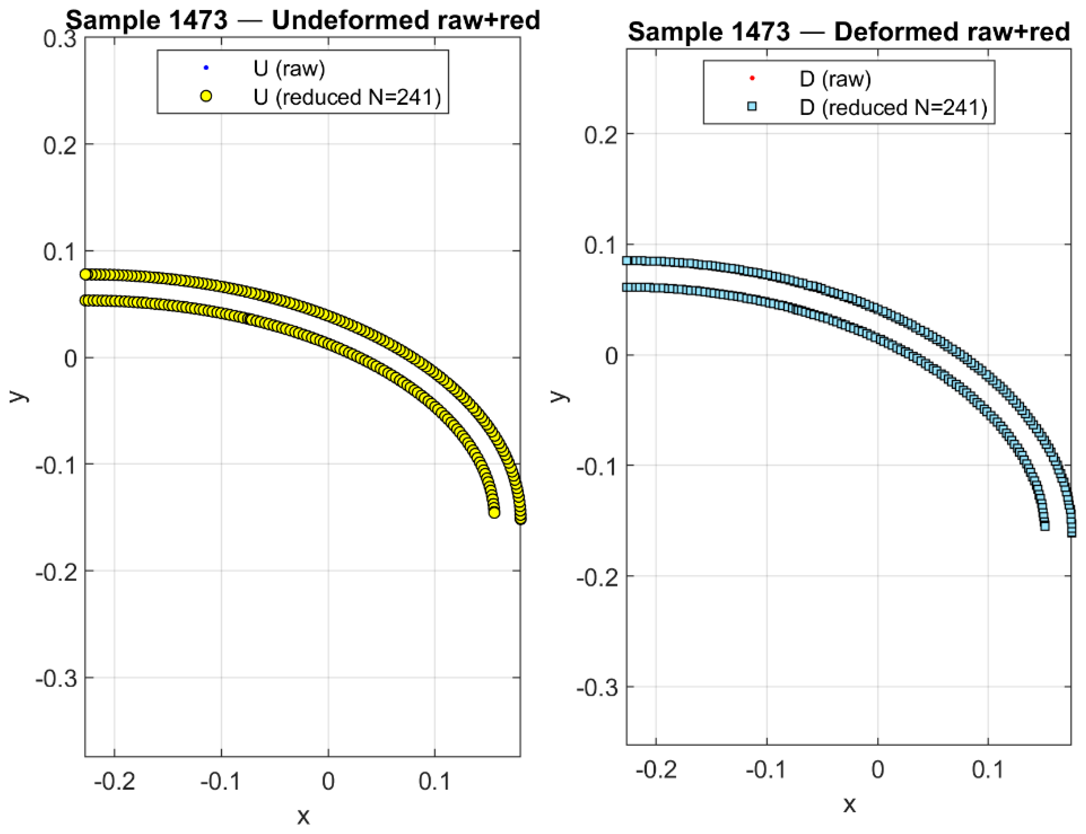
The analysis is organized into four subsections. First, we provide a quantitative evaluation of all tested architectures, reporting standard regression metrics such as root mean squared error (RMSE), coefficient of determination (R²), and correlation coefficients between predicted and ground-truth normalized pressures. Second, we complement these metrics with qualitative visualizations, highlighting representative FEM samples and the corresponding predictions of the neural networks. Third, we conduct a focused sensitivity study, contrasting two modeling stages: (i) a baseline stage where only the undeformed and deformed boundary profiles are provided as inputs, and (ii) an enriched stage where all additional geometric features—namely displacement differences (Δu), normals, and tangents—are incorporated into the node attributes. This comparison clarifies the contribution of mechanics-informed features beyond raw geometry. Finally, we present the architectural evolution and optimization effects, documenting the from enriched GNN to CNN models architectures, and demonstrating how Bayesian hyperparameter optimization improved convergence and predictive stability.

This layered presentation provides not only a rigorous benchmarking of the framework’s predictive capability but also a transparent view of how input representation and network design choices influence inverse load identification performance.

7.1. Quantitative Evaluation—Graph Neural Networks (Boundary-Only Inputs)

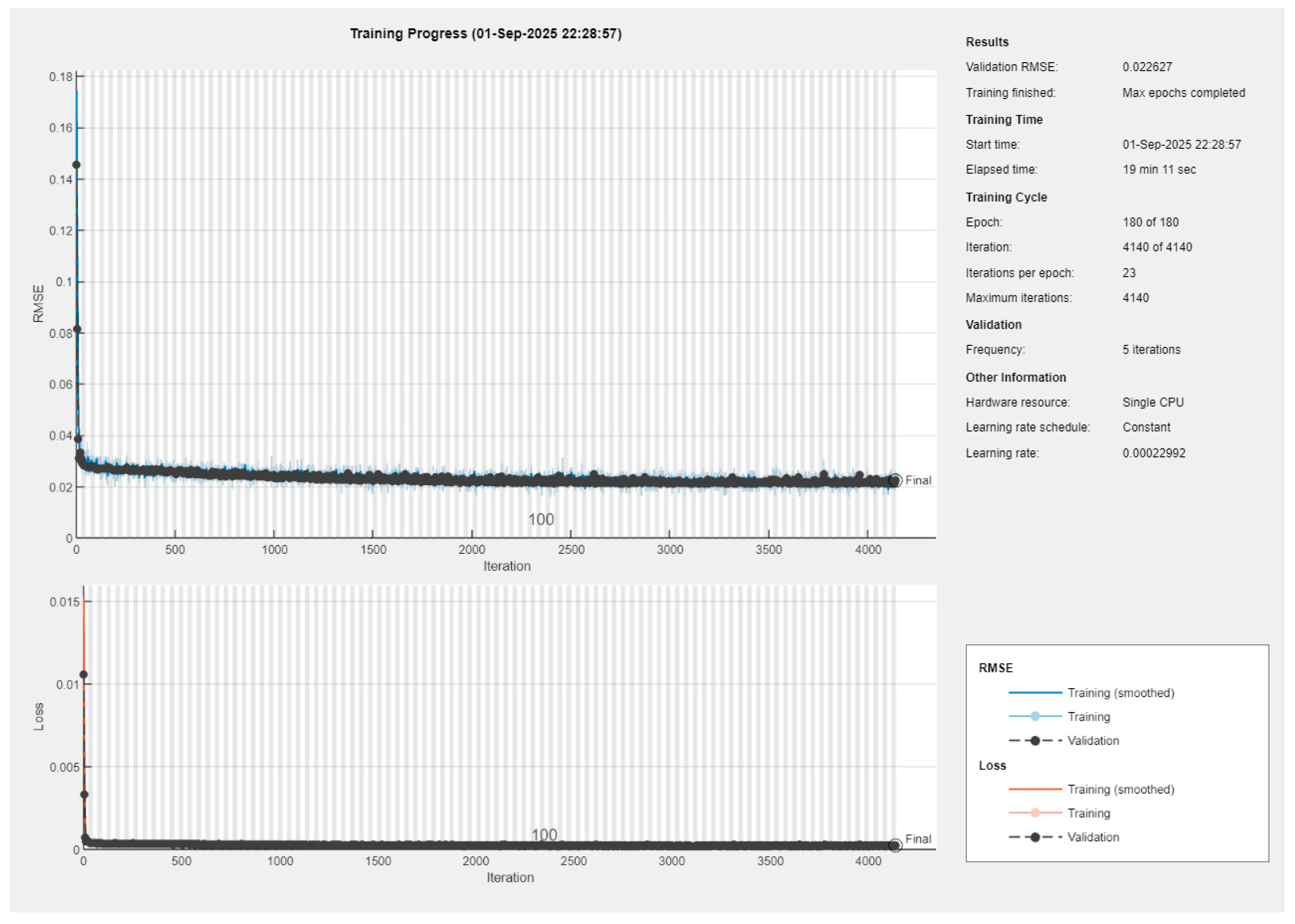
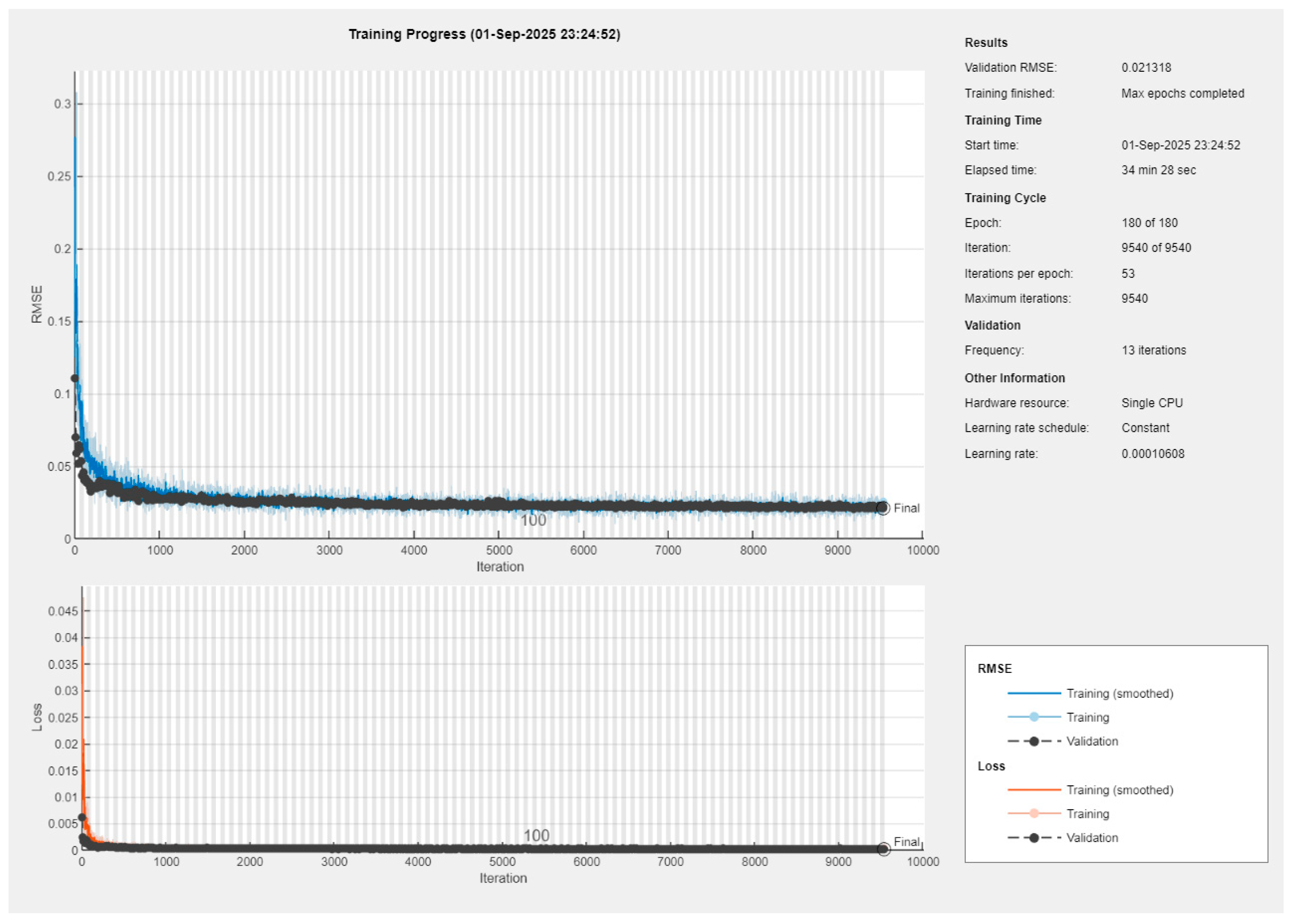
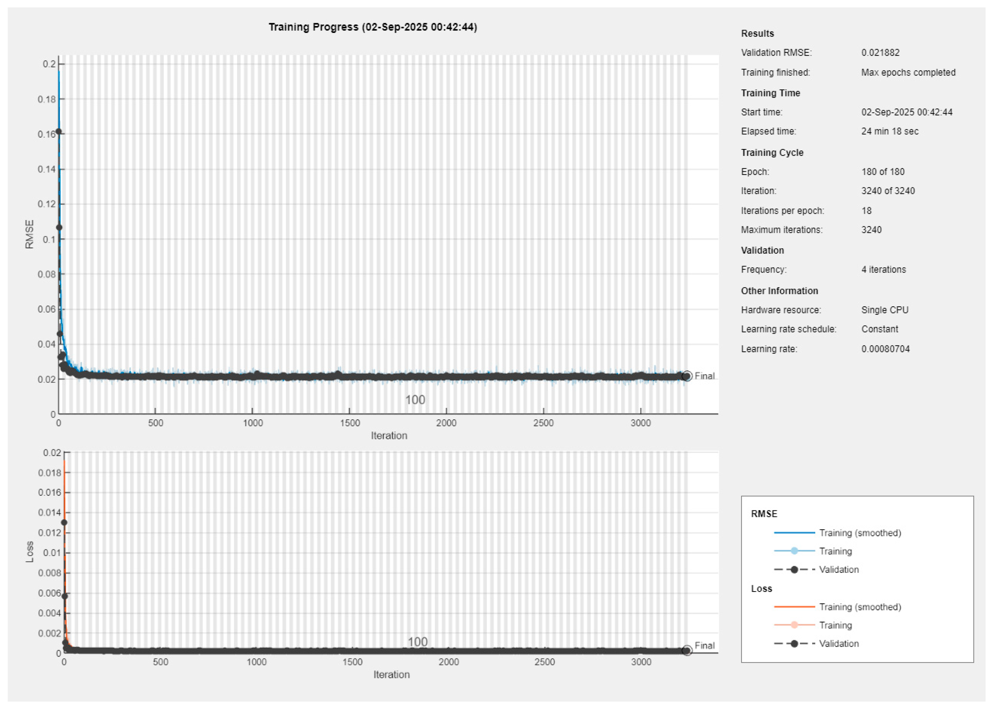
For the GNN models trained with only undeformed and deformed boundary profiles as inputs, the Bayesian-optimized architectures converged to stable and reproducible performance across all splits of the dataset. Training progress curves (see Appendix A) indicated rapid error decay within the first few hundred iterations, followed by a long plateau where both training and validation losses remained nearly parallel. The validation RMSE stabilized around 0.021–0.022 for both internal and external pressures, with negligible divergence from training curves. These learning dynamics confirm that the chosen configurations effectively prevented overfitting while ensuring consistent convergence.

When the input representation was enriched by including additional mechanics-informed features—namely displacement differences (Δu), normals, and tangents—the optimization process identified slightly different architectures for the internal and external pressure regressors. The enriched models maintained the same level of RMSE as the boundary-only baseline but achieved marginally higher correlation with ground-truth pressures and exhibited smoother convergence behavior. This indicates that while the boundary-only setting already provides a strong baseline, the inclusion of enriched features enhances model stability and predictive fidelity, particularly for cases with higher pressure variability.

A comparative summary of the optimized architectures and their final performance is provided in

Table 8. Summary of Bayesian-optimized GNN architectures and performance under two input scenarios: boundary-only versus enriched (boundary + additional features).

Target	Input Type	Optimized Architecture (Selected by BO)	Best BO Objective	Final RMSE (Train/Val/Test)	Pearson r (Range)
$p_{in}$	Boundary-only (undeformed + deformed coords)	Hyperparameters not logged; BO objective stabilized near 0.023	≈0.023	0.0213/0.0219/0.0213	0.63–0.64
$p_{out}$	Boundary-only (undeformed + deformed coords)	Hyperparameters not logged; BO objective stabilized near 0.022	≈0.022	0.0214/0.0215/0.0210	0.62–0.66
$p_{in}$	Enriched (coords + Δu + normals + tangents)	F1 = 121, F2 = 91, F3 = 172; K1 = 3, K2 = 5, K3 = 7; D2 = 3; Blocks = 2; BN = No; Pool = avg; FC1 = 103, FC2 = 183; DropBody = 0.36; DropHead = 0.52; InitLR = 8.07 × 10−4; L2 = 2.47 × 10−5; Batch = 53	0.020509	0.0213/0.0219/0.0213	0.63–0.64
$p_{out}$	Enriched (coords + Δu + normals + tangents)	F1 = 103, F2 = 151, F3 = 251; K1 = 5, K2 = 5, K3 = 3; D2 = 3; Blocks = 2; BN = Yes; Pool = avg; FC1 = 234, FC2 = 190; DropBody = 0.06; DropHead = 0.10; InitLR = 2.83 × 10−3; L2 = 1.34 × 10−4; Batch = 31	0.020714	0.0214/0.0215/0.0210	0.62–0.66

. The table highlights key hyperparameters selected by Bayesian optimization, along with objective values, final RMSE across splits, and correlation ranges. The results show that enriched-input networks yielded marginal improvements in correlation and optimization stability, confirming the added value of physics-informed feature augmentation.

Bayesian optimization selected hyperparameters that balance feature capacity, receptive field, and regularization. Feature dimensions across graph convolution layers ($F_1=121,F_2=91,F_3=172$) and kernel sizes ($K_1=3,K_2=5,K_3=7$) control embedding width and neighborhood size, while depth parameters ($D_2=3, Blocks=2$) define overall network complexity. Average pooling (Pool=avg) and no batch normalization were chosen for aggregation. Two fully connected layers ($F{C}_1=103,F{C}_2=183$) provide dense mappings, with dropout applied at body (0.36) and head (0.52) to reduce overfitting. Training stability was ensured by a small learning rate (8.07 × 10⁻⁴), weight decay (2.47 × 10⁻⁵), and moderate batch size (53). Collectively, these settings illustrate how BO tuned the GNN to achieve stable convergence and low error without over-parameterization.

A comparative summary of the two training processes is provided in

Table 9. Comparative Summary of GNN Training Processes (Boundary-only Inputs).

Metric/Observation	Internal Pressure (pin)	External Pressure (pout)	Notes/Interpretation
Initial RMSE (iteration 1)	~0.32	~0.18	Both start with relatively high errors due to random initialization.
Convergence rate (early decay)	Rapid drop within first ~500 iterations	Rapid drop within first ~300 iterations	Both show steep error decay at the beginning, indicating effective gradient updates.
Validation RMSE (final)	0.0213	0.0215	Nearly identical, showing consistent generalization across tasks.
Training vs. Validation curves	Overlapping, minimal gap	Overlapping, minimal gap	Indicates no overfitting; validation tracks training closely.
Loss stabilization	Plateau after ~1000 iterations, with smooth fluctuations	Plateau after ~800 iterations, slightly noisier tail	Stable convergence in both cases, with marginally smoother dynamics for pin.
Training duration	~34 min (9540 iterations)	~19 min (4140 iterations)	Different iteration counts due to dataset packet size and BO-selected hyperparameters.
Overall robustness	High stability, consistent split performance	High stability, consistent split performance	Both tasks reach the same performance regime; convergence is reliable.

. The table highlights key aspects such as initial error levels, convergence speed, final RMSE values, and differences in training duration between the internal and external pressure networks. Despite minor variations in convergence smoothness and iteration counts, both models ultimately achieved nearly identical validation errors and exhibited stable learning behavior with minimal gap between training and validation curves. This consistency underscores the robustness of the boundary-only GNN baseline and sets the stage for the enriched-feature analysis presented later in Section 7.3.

Quantitatively, the optimized GNN achieved near-identical performance across splits. For internal pressure ($p_{in}$), the final RMSE values were 0.0213 (train), 0.0219 (validation), and 0.0213 (test). For external pressure ($p_{out}$), the respective values were 0.0214, 0.0215, and 0.0210. These small and tightly clustered errors demonstrate both robustness and generalization of the learned mapping.

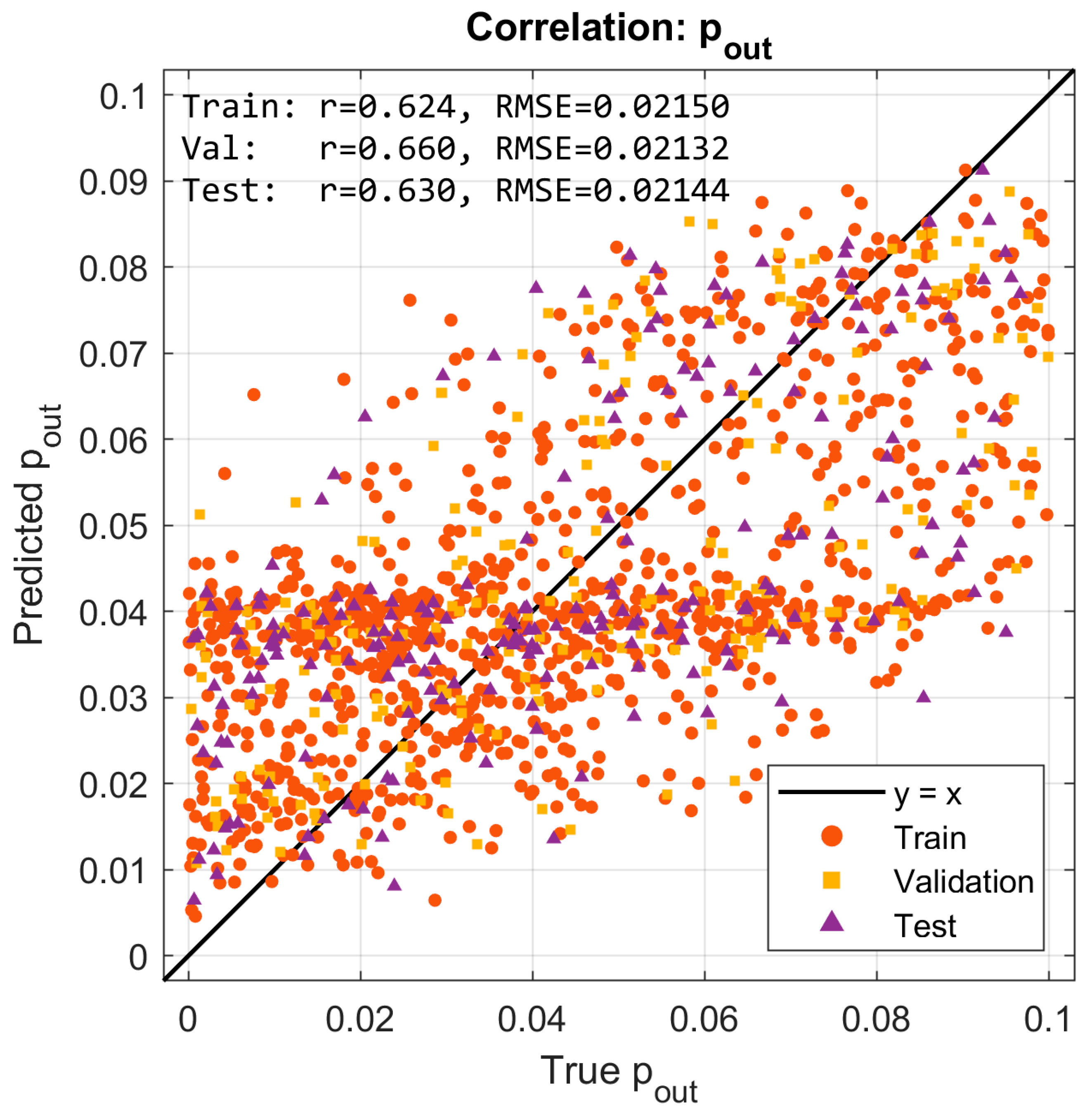
Figure 9 and Figure 10 present scatter plots of predicted versus true normalized pressures for $p_{in}$ and $p_{out}$, respectively. In both cases, the predictions align with the $y=x$ reference line while showing moderate dispersion. Pearson correlation coefficients reached $r\approx 0.63–0.64$ for $p_{in}$ and $r\approx 0.62–0.66$ for $p_{out}$. The moderate correlation values, despite very low RMSE, are consistent with the limited dynamic range of the targets [0, 0.1], where even small absolute deviations significantly affect variance-based statistics. This highlights the importance of reporting both absolute error metrics (RMSE) and relative/normalized measures when interpreting model quality.

The moderate correlation coefficients ($r\approx 0.63–0.66$) should be interpreted in the context of the narrow-normalized pressure range (0–0.1) used in the dataset, which naturally limits statistical variance and reduces the sensitivity of correlation-based metrics. Despite this, the predictions exhibit very low absolute errors and excellent consistency across training, validation, and test sets. Therefore, the slightly reduced $r$-values do not indicate model weakness but rather reflect the compact target domain and the stability of the learned inverse mapping.

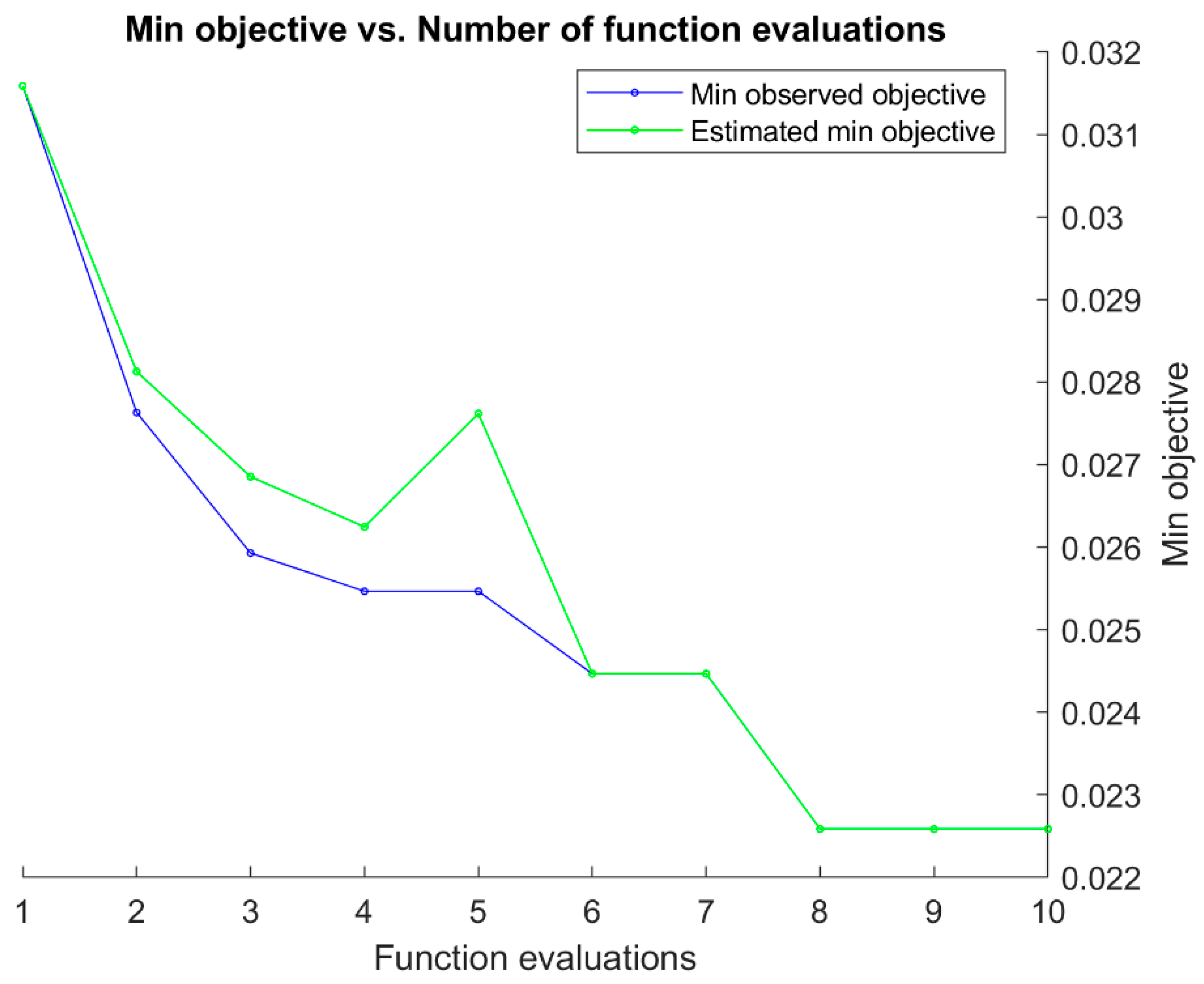
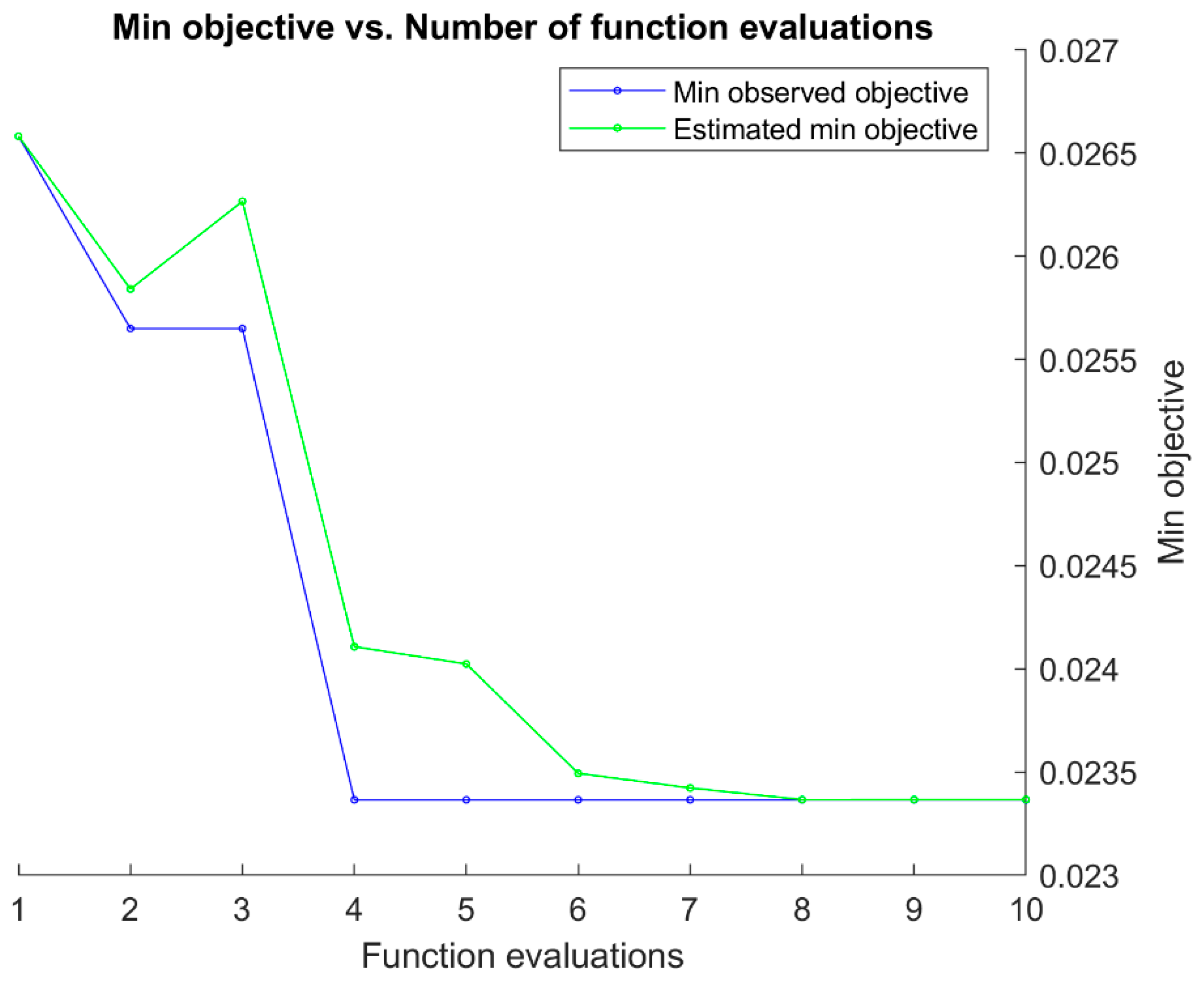
Finally, Figure 11 and Figure 12 summarize the Bayesian optimization (BO) histories for the GNN models targeting $p_{in}$ and $p_{out}$, respectively. In both cases, the minimum observed objective decreases markedly during the first few evaluations and then gradually levels off, stabilizing after approximately 7–8 iterations.

The close agreement between the observed and estimated objective curves further indicates that the surrogate model employed in BO provided accurate guidance during the search. For the $p_{in}$ model, the minimum objective converged near 0.023, while for the $p_{out}$ model it reached approximately 0.022—values consistent with the RMSE reported on the independent validation and test splits. These trajectories demonstrate that BO effectively navigated the hyperparameter space for both networks, yielding architectures that balanced accuracy with stability.

In summary, the boundary-only GNNs for internal and external pressure provide a solid baseline: they achieve low and consistent RMSE across all splits, exhibit stable convergence during training, and yield moderate-to-strong correlation with ground-truth pressures. However, the scatter visible around the $y=x$ line in the correlation plots indicates that relying solely on boundary coordinates leaves some variability unexplained.

By contrast, the enriched-input GNNs—augmented with displacement differences, normals, and tangents—maintain the same low RMSE values while delivering smoother convergence dynamics and slightly higher correlations with the true pressures. These improvements confirm that incorporating mechanics-informed features enhances predictive fidelity and stability, particularly for cases with larger pressure variability. Together, the two configurations establish a clear progression: boundary-only models provide a robust starting point, while enriched models exploit additional geometric and kinematic cues to push performance closer to the limits of the available dataset.

Model accuracy in this study was evaluated using RMSE and Pearson correlation (r), which jointly capture both absolute error magnitude and predictive consistency. These metrics are standard in inverse modeling and were found sufficient to characterize performance across all data splits. Additional measures such as MAE or normalized RMSE were examined during preliminary analysis and showed no new trends; hence, only RMSE and correlation are reported here for clarity and conciseness.

In classical problems with simple geometries—such as spheres or cylinders—the relationship between pressure and displacement can be expressed analytically through closed-form functions. In contrast, the present study deals with nonlinear hyperelastic materials and complex boundary fields, where both the constitutive behavior and geometric mapping are highly nonlinear. Consequently, the relationship between boundary deformations and applied pressures cannot be captured by simple analytical expressions. The adoption of a graph-based neural network thus provides a data-driven means to approximate this intricate mapping, effectively learning the underlying mechanical dependencies that govern the inverse problem.

The stable convergence of the trained GNN models confirms that the network successfully encoded these physical relationships, rather than relying on purely statistical correlations.

7.2. Quantitative Evaluation—Convolutional Neural Networks (CNN)

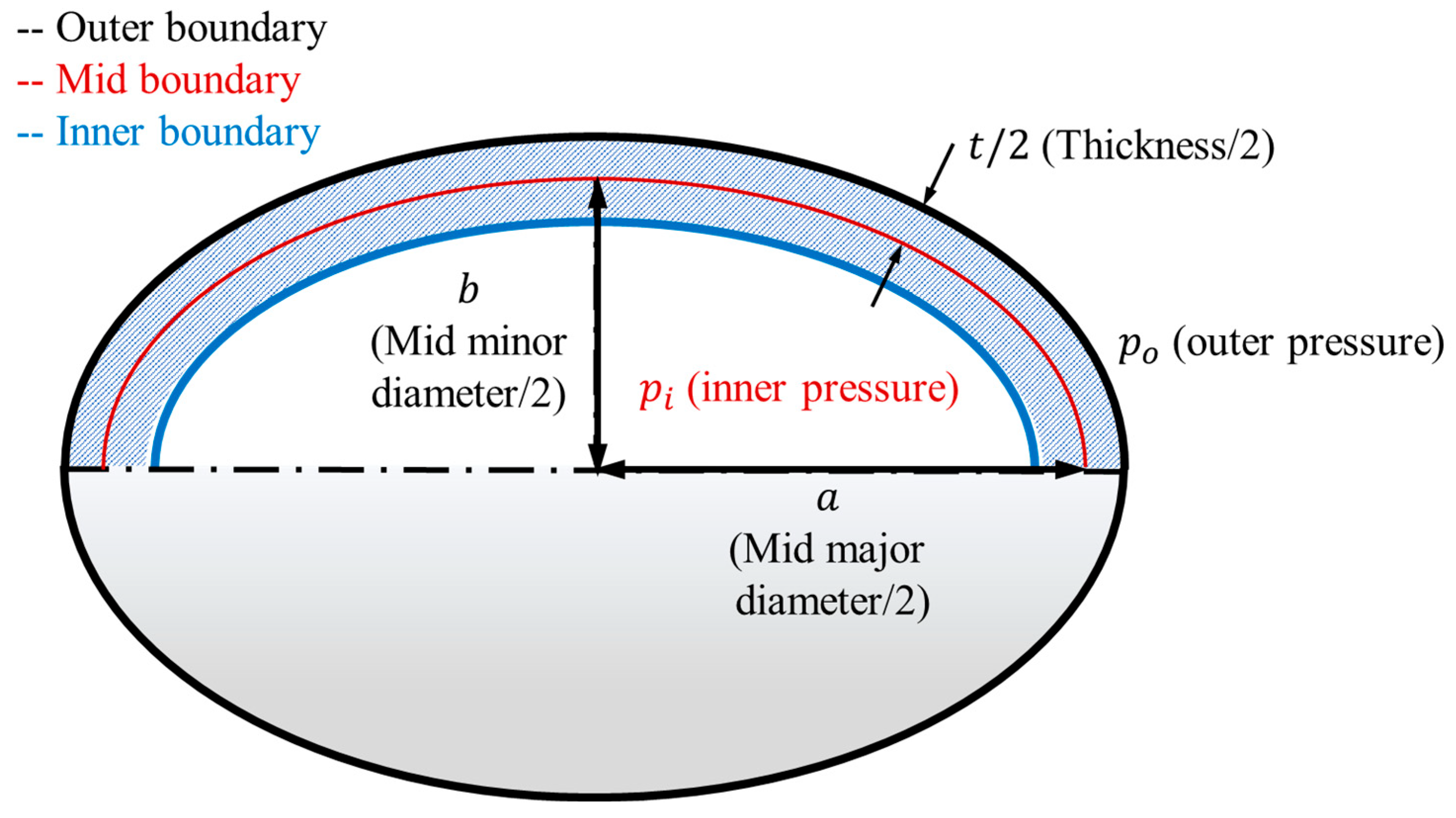
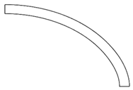
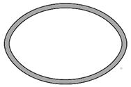
To complement the graph-based models, convolutional neural networks (CNNs) were trained to infer normalized internal and external pressures from FEM-generated deformation data. Unlike GNNs, which operate on resampled boundary graphs, CNNs require structured image representations of the vessel cross-section. Therefore, three input configurations were investigated: (i) quarter-section images capturing local symmetry, (ii) full-ring hollow cross-sections representing the global geometry, and (iii) fully filled cross-sections embedding both inner and outer boundaries within the image domain.

All CNN variants shared a unified architecture consisting of five convolutional blocks followed by two fully connected layers with dropout regularization, and their hyperparameters were tuned using Bayesian optimization. This ensured consistent comparison across different input representations. The following subsections summarize the performance of each CNN configuration and discuss their comparative accuracy and generalization behavior.

The initial experiments employed a conventional CNN architecture consisting of sequential convolutional and pooling layers followed by multiple fully connected layers. However, unlike the GNNs, the CNNs exhibited less satisfactory performance, motivating further exploration of optimized architectures. In particular, the quarter-section configuration showed clear limitations: the predictions tended to collapse toward the mean of the target values for both outputs, indicating that the network failed to capture meaningful correlations between image features and applied pressures.

Given these challenges, the evaluation was extended to full-ring and filled-section inputs, which provide more global geometric information and deformation context. The following subsections present the results for these input types, together with an assessment of underfitting and overfitting behaviors observed during training, and a discussion of how architectural refinements affect predictive accuracy.

Although Bayesian optimization was employed to systematically refine the CNN architectures across all input variants and establish a balanced baseline for comparison with GNNs, additional aspects—such as geometric or intensity-based data augmentation and controlled noise-perturbation studies—could further improve the interpretability and robustness of the CNN results. These complementary analyses fall outside the scope of the present work but are identified as valuable directions for future research, where a more comprehensive assessment of CNN sensitivity to sampling variability and feature perturbations will be undertaken.

7.2.1. CNN with Full-Ring Cross-Section Inputs

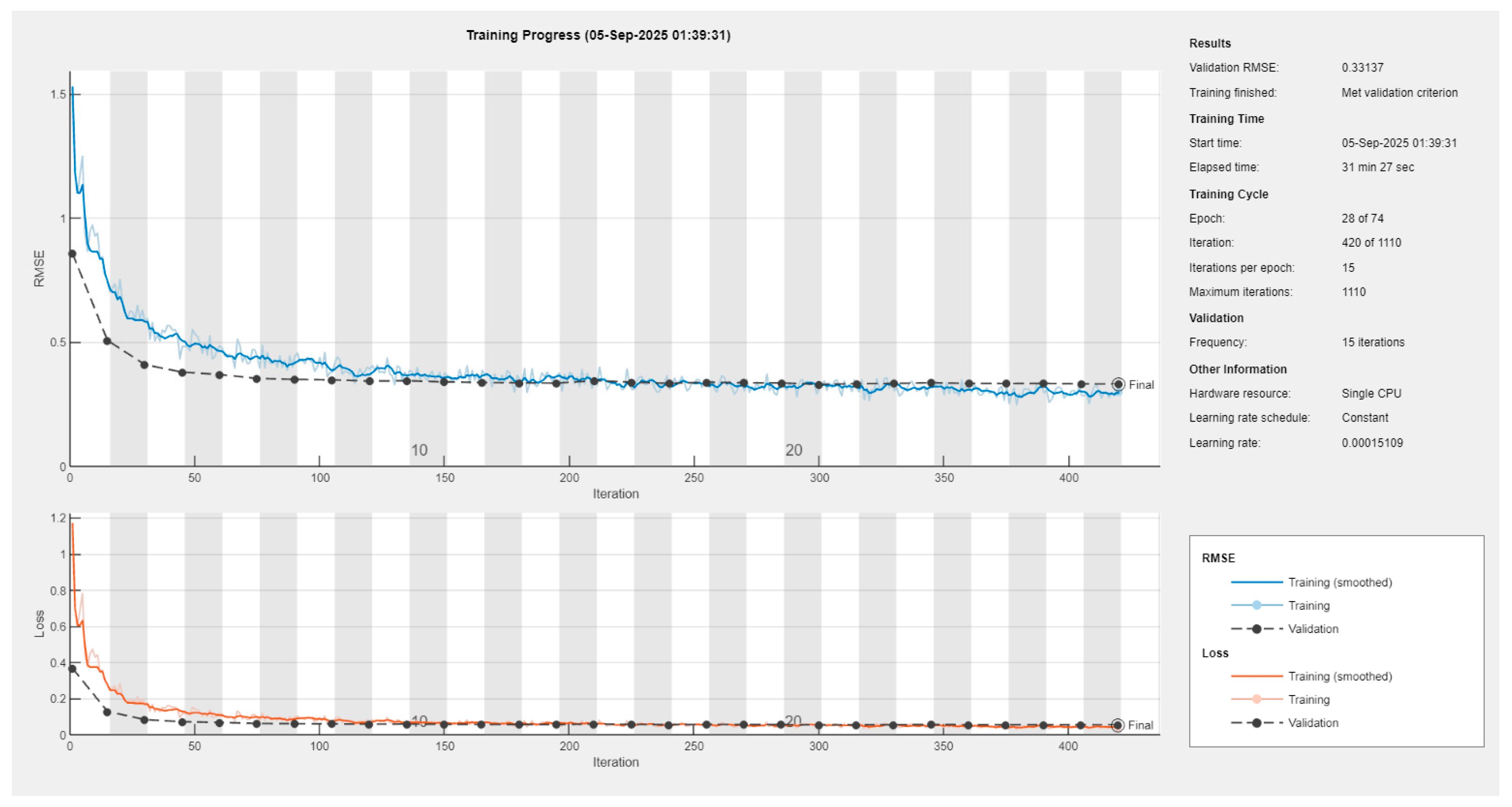
For the full-ring image inputs, the CNN architecture was optimized through Bayesian hyperparameter search. The best-performing model adopted five convolutional blocks with a filter schedule starting at 19 channels and growing modestly per block. The convolutional stack was followed by two fully connected layers (333 and 259 neurons), with dropout regularization applied at rates of 0.20 and 0.14, respectively. The optimization also selected a relatively small learning rate (1.5 × 10⁻⁴), weak $L_2$ regularization (6.3 × 10⁻⁶), and a batch size of 64, converging within 74 epochs.

Training curves (see Appendix A) demonstrate rapid decay in both training and validation loss during the initial epochs, followed by stabilization around epoch 25–30. The validation RMSE plateaued near 0.0228 (mean of two outputs), which is notably lower than the unoptimized CNN but still above the performance levels achieved by GNNs. Importantly, overfitting was mitigated by the selected configuration: the validation error remained close to the training error, in contrast to earlier trials where the network memorized training images and failed to generalize.

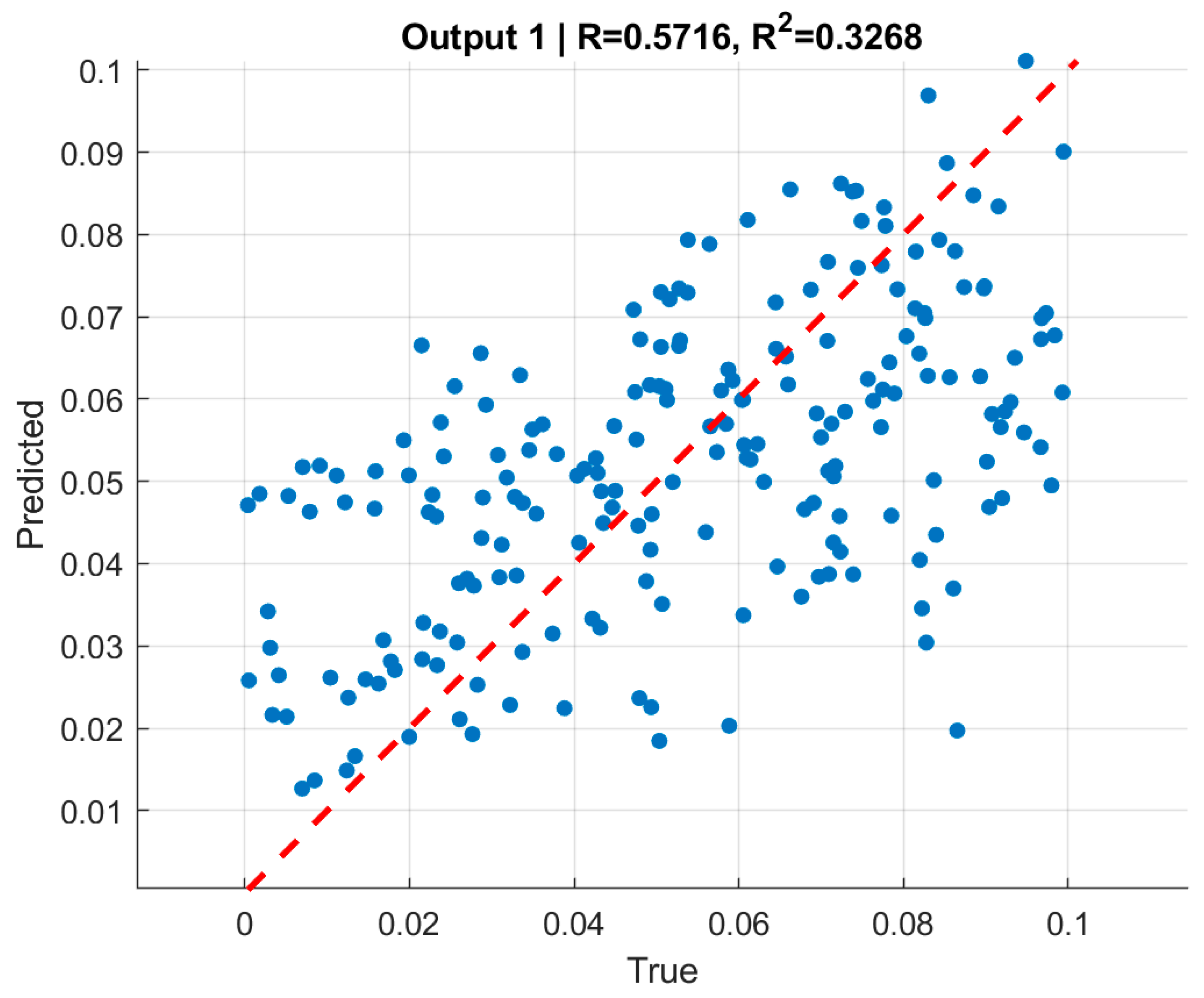
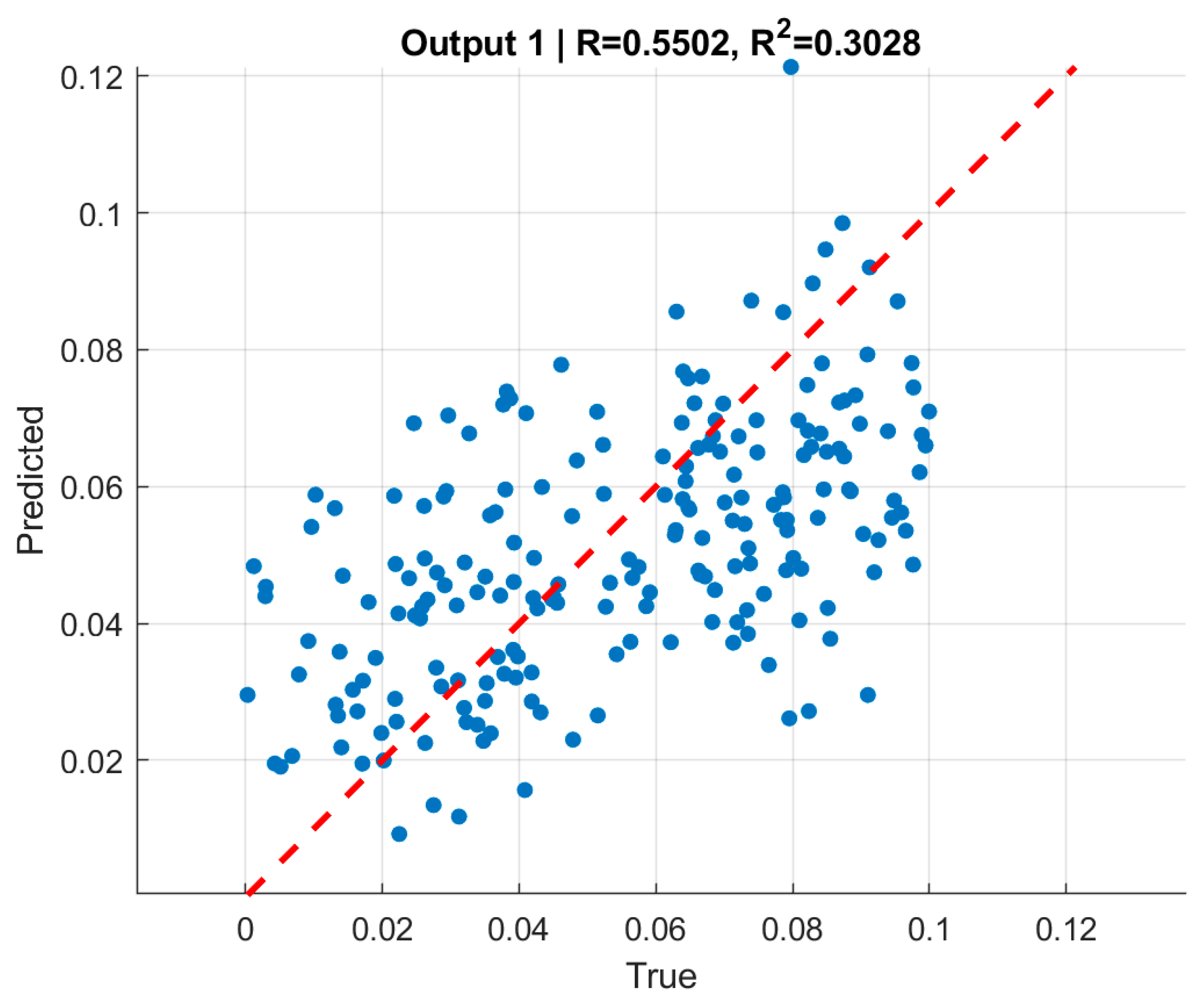
Across datasets, the model showed consistent but modest predictive power as given in

Table 10. Performance metrics of Optimized CNN for full-ring input.

Dataset	RMSE (Output 1)	RMSE (Output 2)	Mean RMSE	R2 (Output 1)	R2 (Output 2)
Validation	0.0225	0.0242	0.0234	0.316	0.283
Test	0.0230	0.0249	0.0239	0.267	0.130

. On the validation set, RMSE values were 0.0225 and 0.0242 for the two outputs, corresponding to R² values of 0.316 and 0.283. On the test set, RMSE values were 0.0230 and 0.0249, with corresponding R² values dropping to 0.267 and 0.130, respectively. Scatter plots of true versus predicted values (Figure 13, Figure 14, Figure 15 and Figure 16) illustrate these findings: while the predictions cluster around the regression line, the dispersion is considerable, reflecting the limited explanatory capacity of CNNs compared to the graph-based approach.

7.2.2. CNN Architecture (Full-Ring Hollow Cross-Section Input)

The optimized CNN architecture for hollow full-ring images was composed of five convolutional blocks, starting with 19 filters in the first layer and gradually increasing through subsequent layers. This design enabled the network to capture both local boundary details and global deformation patterns around the ring. The convolutional backbone was followed by two fully connected layers of sizes 333 and 259 neurons, which provided sufficient representational capacity for mapping high-level image features to pressure predictions. To prevent overfitting, dropout layers with moderate rates (0.20 in the body and 0.14 at the head) were included, complemented by a small L₂ regularization coefficient (6.3 × 10⁻⁶). Training used the Adam optimizer with a batch size of 64 and an initial learning rate of 1.5 × 10⁻⁴, converging within ~74 epochs. This configuration produced stable learning dynamics and improved generalization compared to the unoptimized baseline CNN.

In summary, the CNN trained on full-ring images benefited from architectural optimization, achieving substantially lower RMSE compared to the baseline and avoiding severe overfitting. However, the relatively low R² values—particularly on the test set—underscore persistent challenges in capturing the nonlinear mapping from cross-sectional images to applied pressures. These results suggest that although CNNs can exploit global cross-sectional patterns, their predictive performance remains inferior to GNNs operating directly on boundary-derived features.

7.2.3. CNN with Fully Filled Cross-Section Inputs

The third CNN configuration employed fully filled cross-sectional images of the vessel, in which both inner and outer boundaries were embedded within a solid domain. This representation was intended to provide the network with a richer spatial encoding of geometry and deformation compared to boundary-only images.

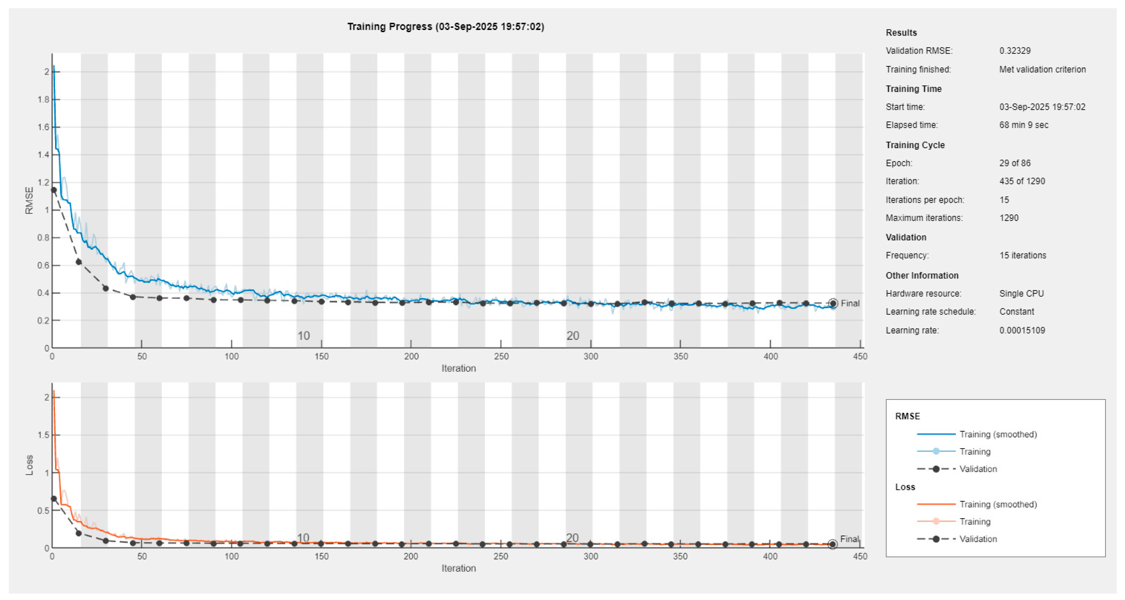
Bayesian optimization was again used to tune the architecture and hyperparameters. The final model adopted five convolutional layers with filter sizes growing moderately, followed by two fully connected layers with 300+ neurons each. Dropout layers (≈0.2) and a small L₂ regularization term (7 × 10⁻⁶) were included to mitigate overfitting, while the learning rate (1.5 × 10⁻⁴) and batch size (64) were selected to ensure stable convergence. Training proceeded for ~86 epochs until the validation criterion was reached (see Appendix A).

The learning dynamics demonstrated consistent reduction in both training and validation RMSE during the first 20–30 epochs, after which both curves plateaued. The final validation RMSE stabilized around 0.032, which is noticeably higher than the full-ring CNN but still an improvement compared to the quarter-section case. Importantly, validation and training curves remained close throughout training, indicating that overfitting was controlled effectively.

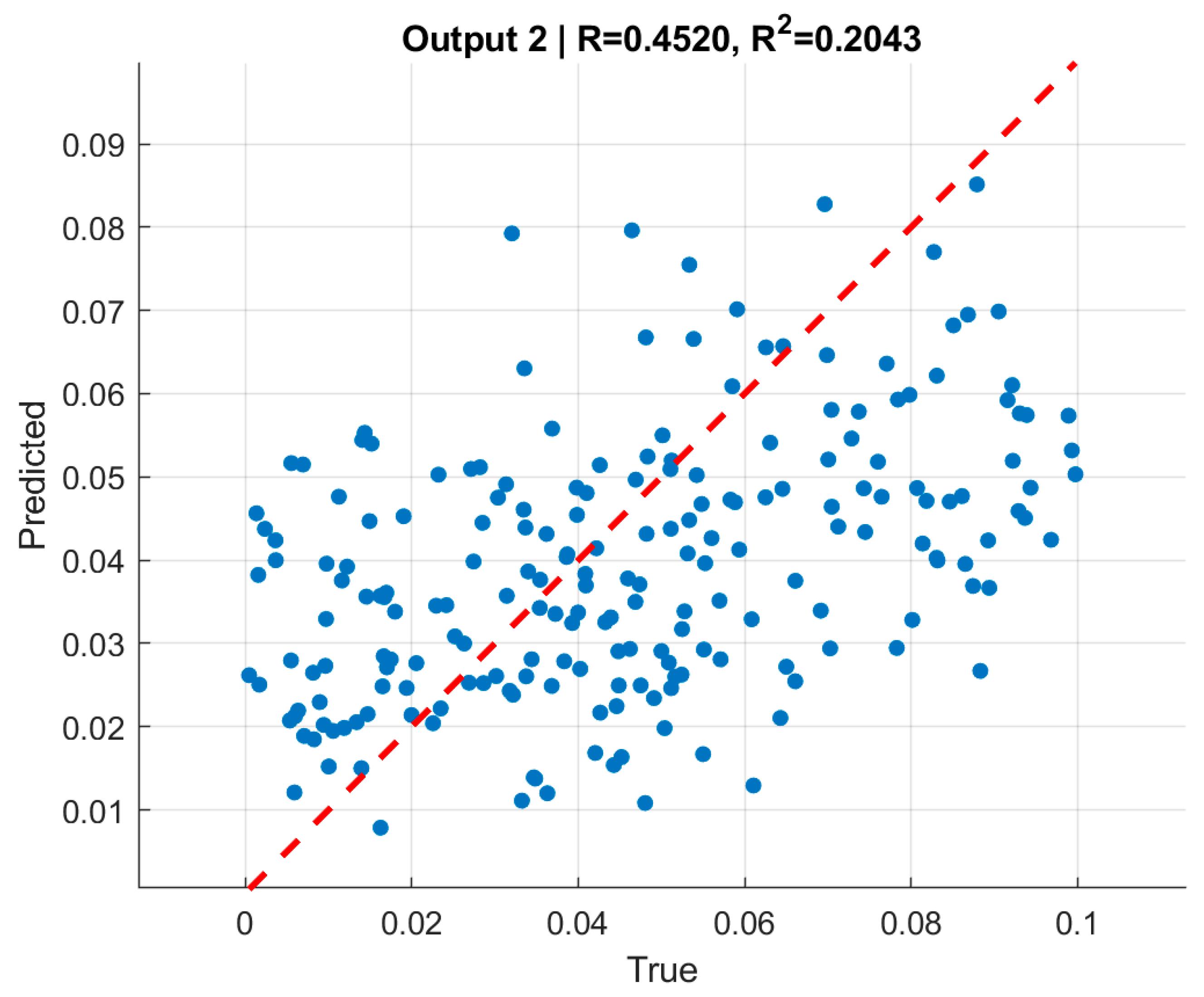
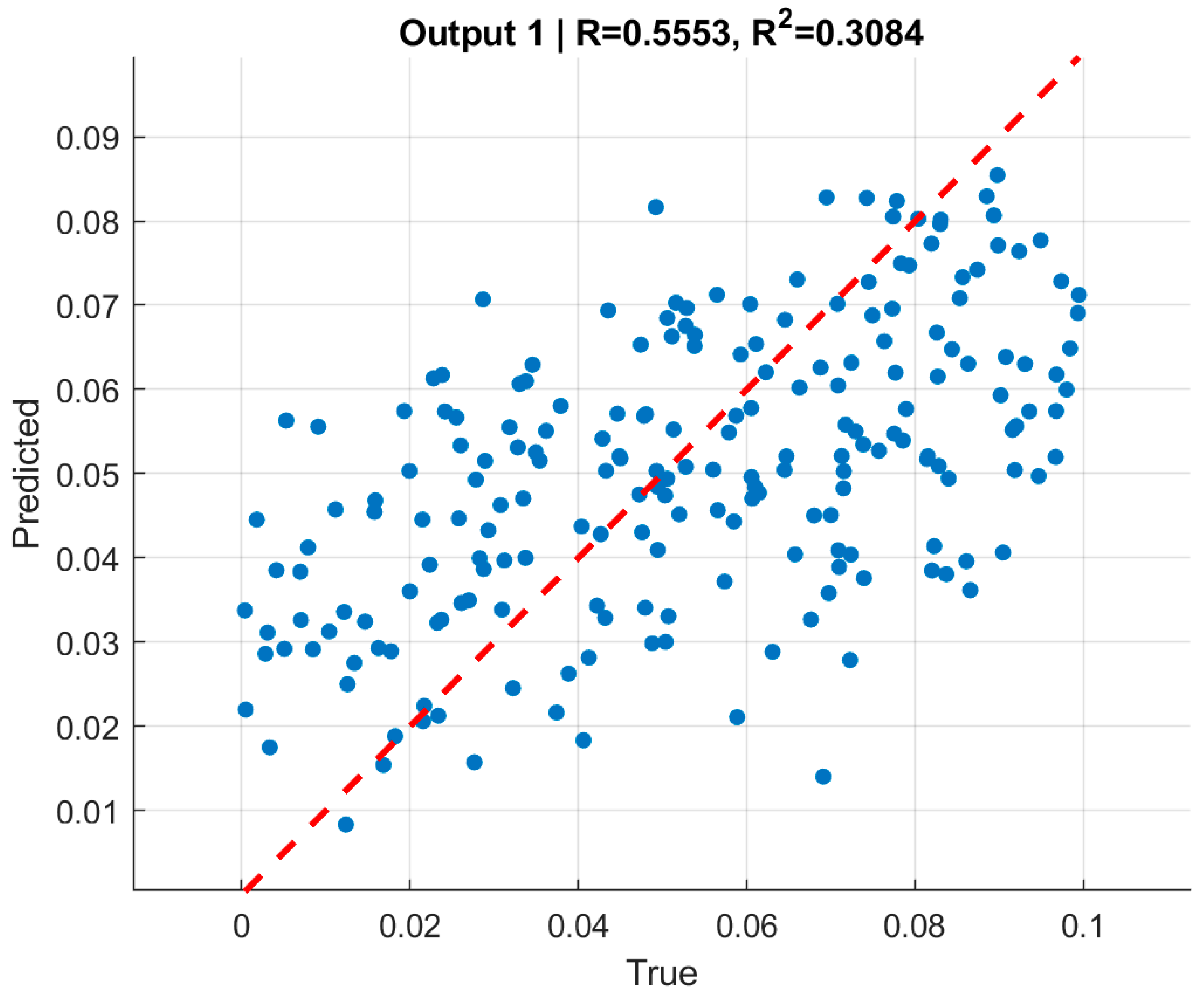
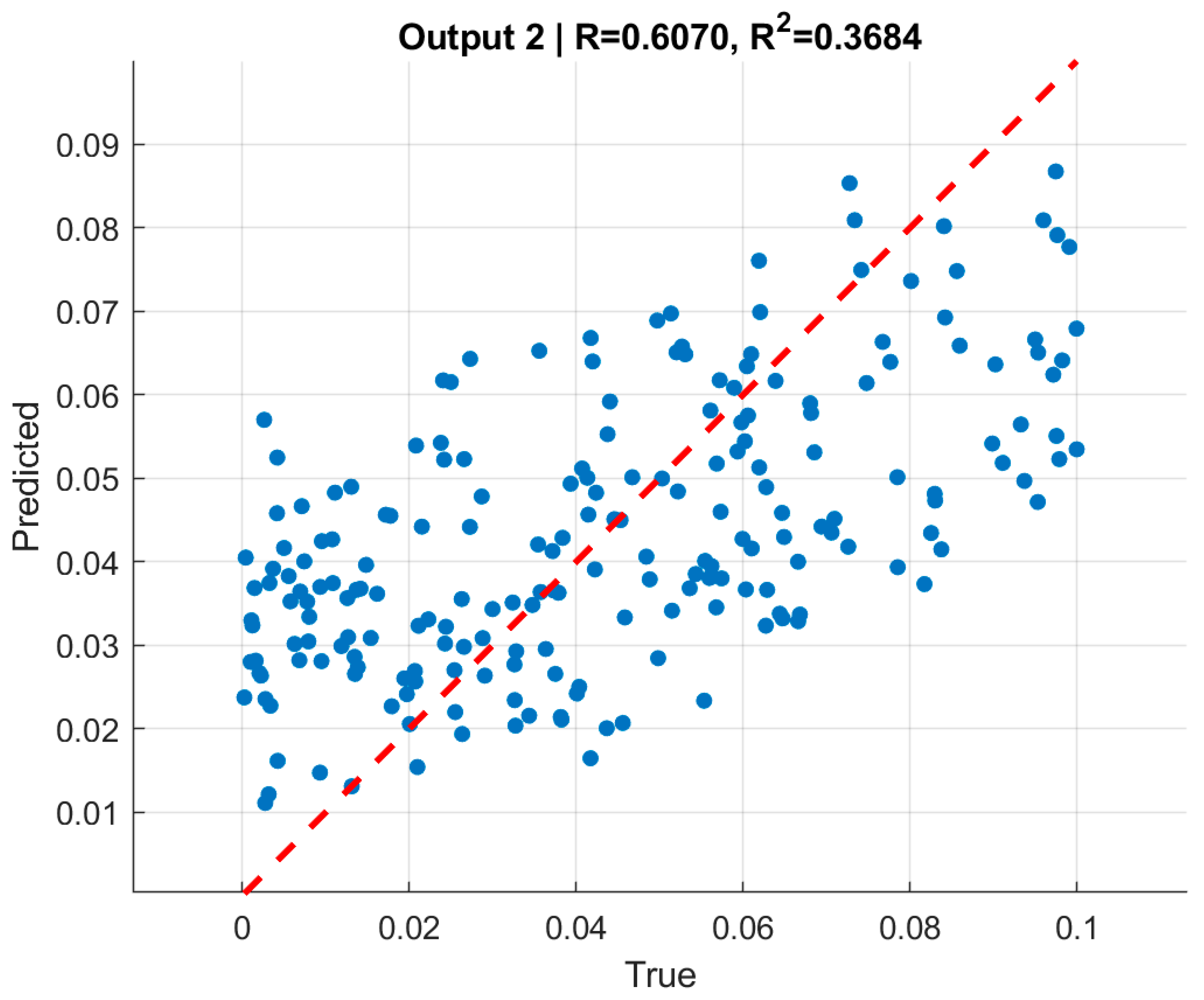
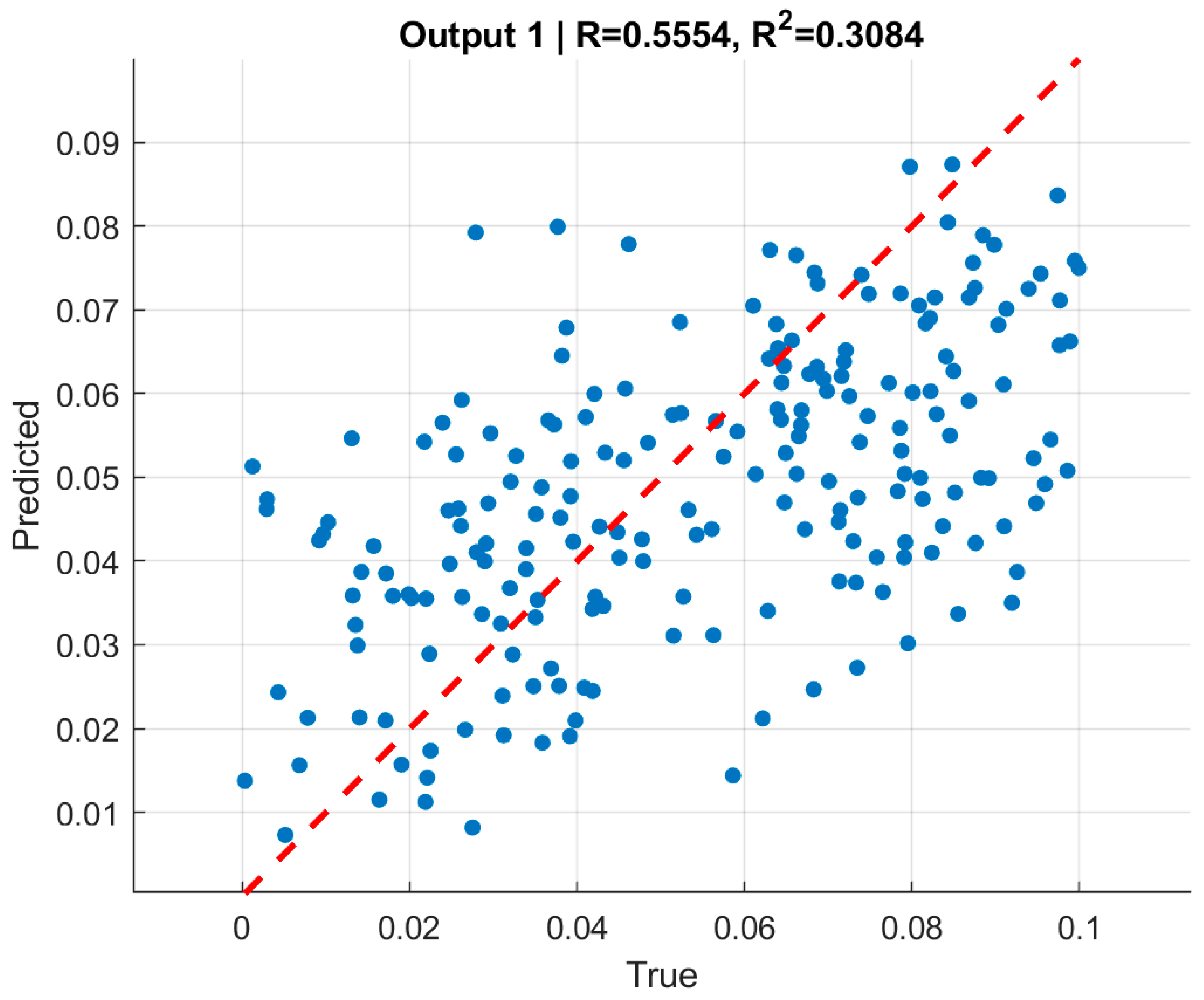
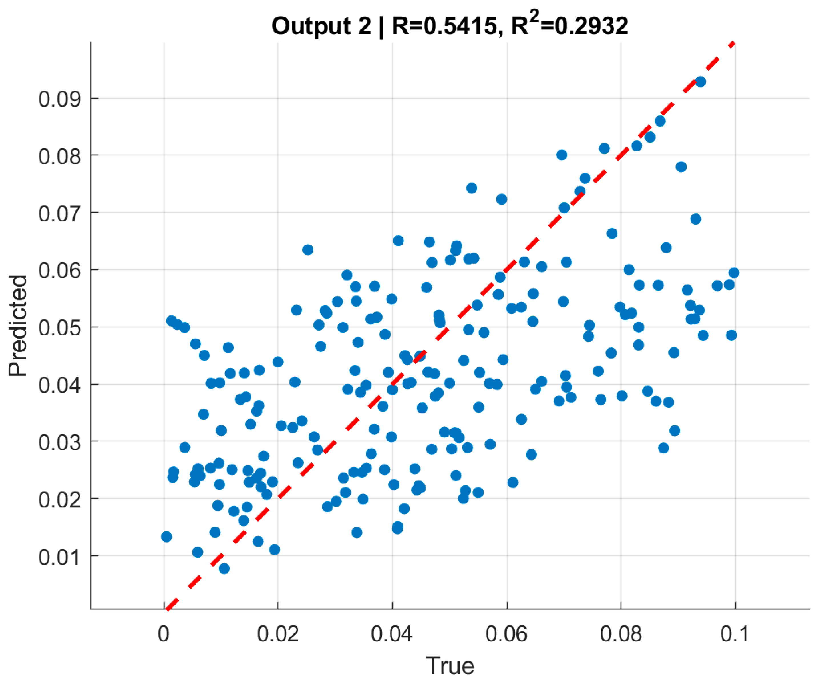
Performance metrics reflected this behavior are shown in Table 8. On the validation set, the RMSE values were 0.028–0.032 for the two outputs, with corresponding R² values of 0.308 and 0.368. On the test set, the network achieved comparable RMSE levels (0.029–0.031), while R² values remained modest at 0.308 and 0.293, respectively. Scatter plots of predicted versus true pressures (Figure 17, Figure 18, Figure 19 and Figure 20) confirm that the CNN was able to capture global deformation trends, but the predictions were dispersed around the regression line, reflecting limited explanatory accuracy compared to GNNs.

7.2.4. CNN Architecture (Filled Cross-Section Input)

The optimized CNN architecture for filled cross-section images employed five convolutional layers with progressively increasing filter numbers, enabling hierarchical extraction of deformation features from the vessel geometry. This convolutional backbone was followed by two fully connected layers of approximately 300 neurons each, designed to integrate high-level spatial features into pressure predictions. To mitigate overfitting, dropout layers with rates around 0.2 were included, along with a small L₂ weight penalty (7 × 10⁻⁶). Training was performed with a batch size of 64 and an initial learning rate of 1.5 × 10⁻⁴, using the Adam optimizer. Convergence was achieved after ~86 epochs, yielding balanced performance across training and validation sets without severe divergence.

In summary, the fully filled input representation enabled the CNN to achieve more stable and generalizable performance than the quarter-section case, with test metrics comparable to validation results. Nevertheless, despite architectural optimization, the CNN struggled to capture fine-scale correlations between deformation fields and applied pressures, as reflected in the relatively low R² values, as shown in

Table 11. Optimized CNN architecture (filled cross-section input) and performance metrics.

Dataset	RMSE (Output 1)	RMSE (Output 2)	Mean RMSE	R2 (Output 1)	R2 (Output 2)
Validation	0.0280	0.0320	0.0300	0.308	0.368
Test	0.0290	0.0310	0.0300	0.308	0.293

. This reinforces the conclusion that boundary-informed GNNs provide a more effective framework for inverse pressure identification in hyperelastic vessels.

7.3. Qualitative Metrics

In addition to the quantitative indicators of performance such as RMSE and R², qualitative analyses were conducted to visually assess the predictive behavior of the trained models. Scatter plots comparing true versus predicted pressures for both GNN and CNN frameworks revealed clear differences in fidelity and generalization. For the GNNs, the predicted points clustered closely around the y = x line, with only moderate scatter, demonstrating their ability to capture nonlinear deformation–pressure relationships in a stable manner. In contrast, the CNN models—particularly those trained on quarter-section images—exhibited broader dispersion and a tendency to regress toward average values, highlighting their limited capacity to resolve detailed deformation cues.

Visualizations of selected vessel cross-sections further reinforced these trends. For cases with pronounced deformations, the GNNs provided consistent pressure predictions aligned with FEM ground-truth values, while the CNNs frequently underestimated or overestimated loads, especially in near-spherical configurations. These qualitative observations complement the quantitative metrics, underscoring that GNNs not only achieve lower numerical errors but also deliver predictions that are physically more coherent with observable deformation patterns.

Classical inverse techniques such as regularized least squares and adjoint-based sensitivity analyses have long been employed for load identification problems. However, their direct application to nonlinear hyperelastic systems with dual pressure boundaries would require problem-specific regularization and iterative forward–inverse coupling, leading to high computational cost and potential instability.

The present work instead focuses on establishing a machine-learning-based baseline capable of learning the inverse mapping directly from high-fidelity FEM data. This provides a foundation upon which future studies can incorporate or benchmark against classical optimization-based inversions. Such extensions, including hybrid GNN–adjoint or physics-informed variants, are currently being explored as part of ongoing work.

The observed correspondence between boundary displacements and identified pressures is consistent with classical elasticity theory, confirming that the learned GNN mappings capture physically meaningful relationships. Larger radial displacements and outward normal deformations were consistently associated with higher internal pressure, while variations in tangential components reflected the redistribution of hoop stress along the vessel wall. This behavior is physically consistent with hyperelastic theory, in which the nonlinear strain–energy relation governs the equilibrium between internal and external pressures. The stable convergence of the GNN models therefore indicates that the network effectively captured this underlying mechanical relationship, rather than learning purely statistical correlations.

8. Conclusions

This study introduced a Graph-FEM/ML framework for inverse load identification in thick-walled hyperelastic pressure vessels, in which measurable boundary deformations were used to predict normalized internal and external pressures. A comprehensive FEM-generated dataset of 1386 valid samples was created through Latin Hypercube Sampling, spanning a wide range of geometric and loading conditions. Two complementary learning strategies were examined: graph neural networks (GNNs), operating directly on resampled and feature-enriched boundary data, and convolutional neural networks (CNNs), trained on image-based cross-sections of undeformed and deformed vessel geometries.

Quantitatively, the GNNs achieved low and stable root-mean-square errors (≈2 × 10⁻²) across training, validation, and test sets, confirming their robustness and generalization capability. When enriched with mechanics-informed features—such as displacement differences, normal and tangent vectors—their predictive correlation further improved, demonstrating the benefit of embedding physically meaningful descriptors into the learning process. In contrast, CNN models showed limited generalization: quarter-section inputs regressed toward mean values, while full-ring and filled-section representations improved after Bayesian optimization yet remained less accurate than the GNNs. These results highlight the superior capacity of graph-based architectures to capture nonlinear relationships between boundary deformations and dual pressure fields.

From a computational standpoint, the trained GNNs performed inverse inference in less than 0.02 s per sample—over three orders of magnitude faster than traditional iterative FEM-based inversions—underscoring the efficiency of the proposed data-driven approach for potential real-time or embedded applications. The physically consistent correspondence observed between boundary displacements and identified pressures confirms that the learned GNN mappings adhere to classical elasticity principles rather than purely statistical correlations.

In summary, boundary-informed GNNs consistently outperformed CNNs in reconstructing load conditions from deformation data, owing to their ability to exploit graph-structured FEM information and to capture the nonlinear coupling between boundary displacements and applied pressures. This establishes a robust, scalable, and computationally efficient paradigm that bridges high-fidelity finite-element simulations with machine-learning models, enabling rapid and physically consistent inverse load identification. The proposed framework lays the groundwork for future extensions toward noise-resilient learning, more complex constitutive laws (e.g., Mooney–Rivlin or Ogden), and non-axisymmetric or experimentally measured geometries, ultimately advancing data-driven mechanics toward real-time structural sensing and diagnostic applications.

Limitations and Future Work

While the proposed Graph-FEM/ML framework demonstrated robust and consistent performance on synthetic hyperelastic data, several important aspects remain to be explored. Due to time and computational constraints during the current revision cycle, additional investigations—such as noise-perturbed deformation inputs, sensitivity analyses with alternative hyperelastic constitutive laws (e.g., Mooney–Rivlin or Ogden models), and benchmarking against classical inverse solvers (e.g., least-squares or adjoint-based formulations)—could not be incorporated. These directions are essential for extending the generalizability and physical interpretability of the framework and are currently underway as part of our ongoing research.

Furthermore, geometric or intensity-based data augmentation for the CNN models, as well as controlled noise-injection studies to assess their robustness to sampling variability, were not included in this version due to the substantial computational cost associated with retraining and re-optimizing multiple CNN architectures. Future work will include a systematic robustness analysis of the CNN baselines using well-defined augmentation and noise strategies to enable a more balanced and comprehensive comparison with the GNN models. These extensions will provide deeper insight into the representational limitations of grid-based architectures and strengthen the overall evaluation of inverse load identification methods.