Author Contributions
Conceptualization, S.W. and Y.Z.; data curation, S.W. and F.Z.; formal analysis, S.W. and Y.Z.; funding acquisition, S.W.; investigation, S.W. and B.L.; methodology, S.W. and B.L.; project administration, Y.Z.; resources, S.W. and Y.Z.; software, S.W.; supervision, Y.Z.; validation, S.W., B.L. and F.Z.; visualization, S.W.; writing—original draft, S.W.; writing—review and editing, S.W., B.L., F.Z. and Y.Z. All authors have read and agreed to the published version of the manuscript.
Figure 1.
The proposed enhanced YOLOv8 architecture for PCB defect detection integrates three key components: Dual-Domain Convolution (DD-Conv) modules, Global–Local Axial Attention (GLA-Attention) blocks, and Cross-Stage Partial with Dynamic Shifted Large Kernel Convolution (C2f-DSLKConv) modules. The architecture comprises (a) a C2f-DSLKConv backbone for hierarchical feature extraction, (b) a PANet neck enabling multi-scale feature fusion through bidirectional pathways, (c) multi-level detection heads for simultaneous bounding box regression and classification, (d) C2f modules for efficient feature aggregation with enhanced gradient flow, (e) CBS blocks (Convolution-BatchNorm-SiLU) for fundamental feature transformation, and (f) SPPF (Spatial Pyramid Pooling-Fast) for multi-scale context aggregation. This frequency–spatial learning framework simultaneously captures spatial and frequency-domain characteristics, yielding improved detection accuracy and computational efficiency.
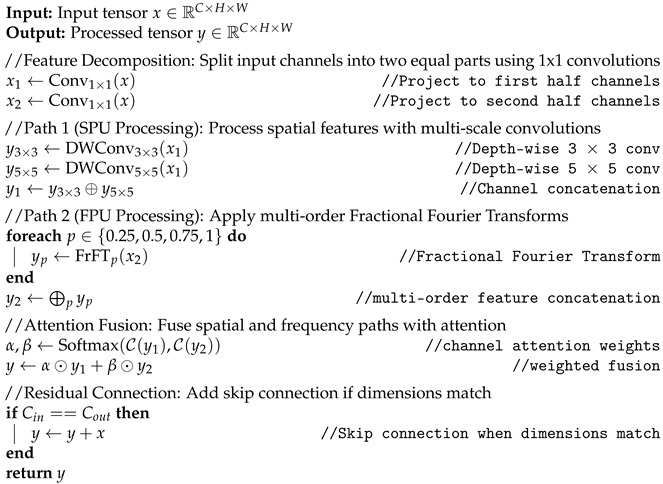
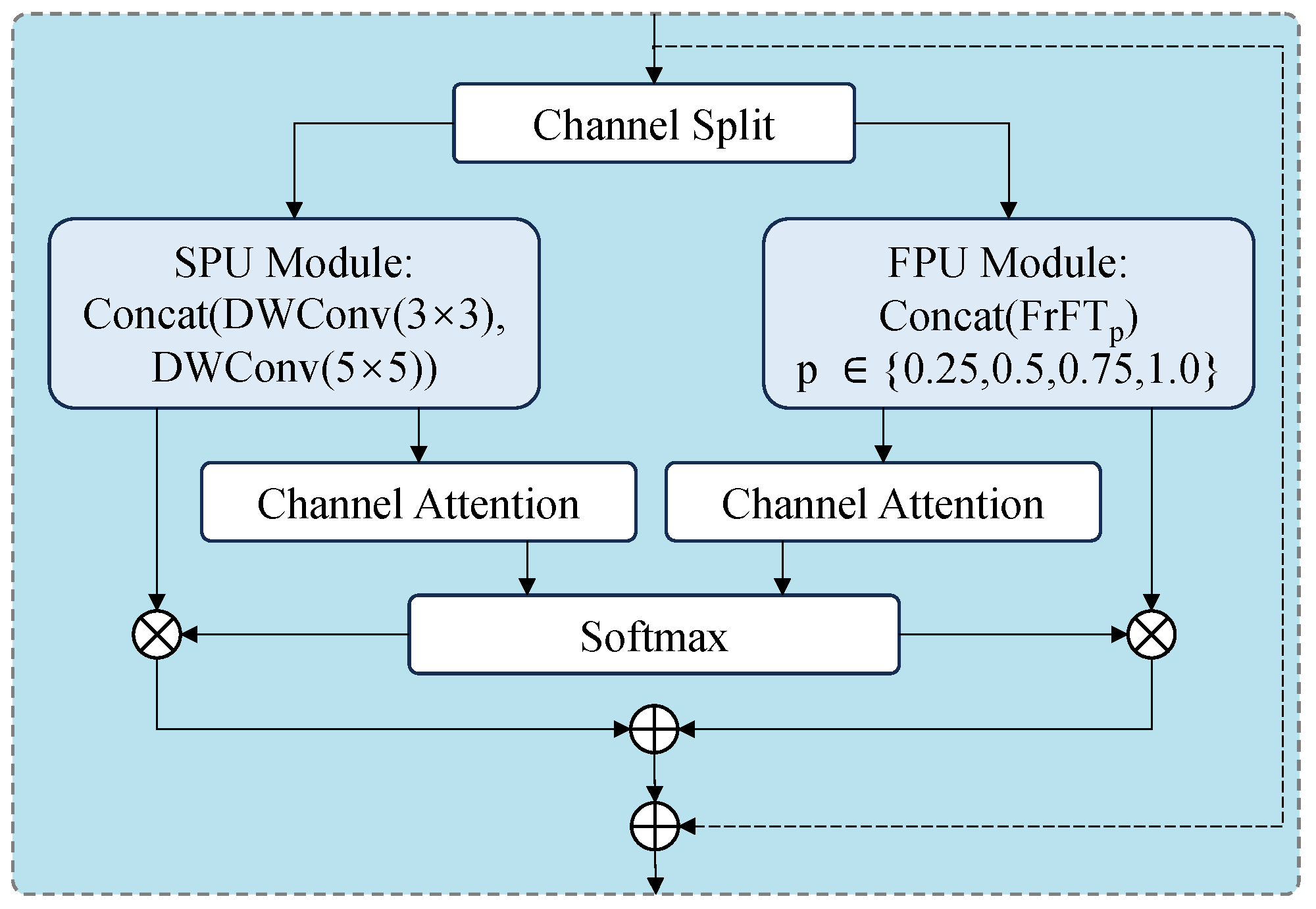
Figure 2.
Architecture of the proposed DD-Conv module. Dashed line indicates residual connection when input/output channels match.
Figure 2.
Architecture of the proposed DD-Conv module. Dashed line indicates residual connection when input/output channels match.
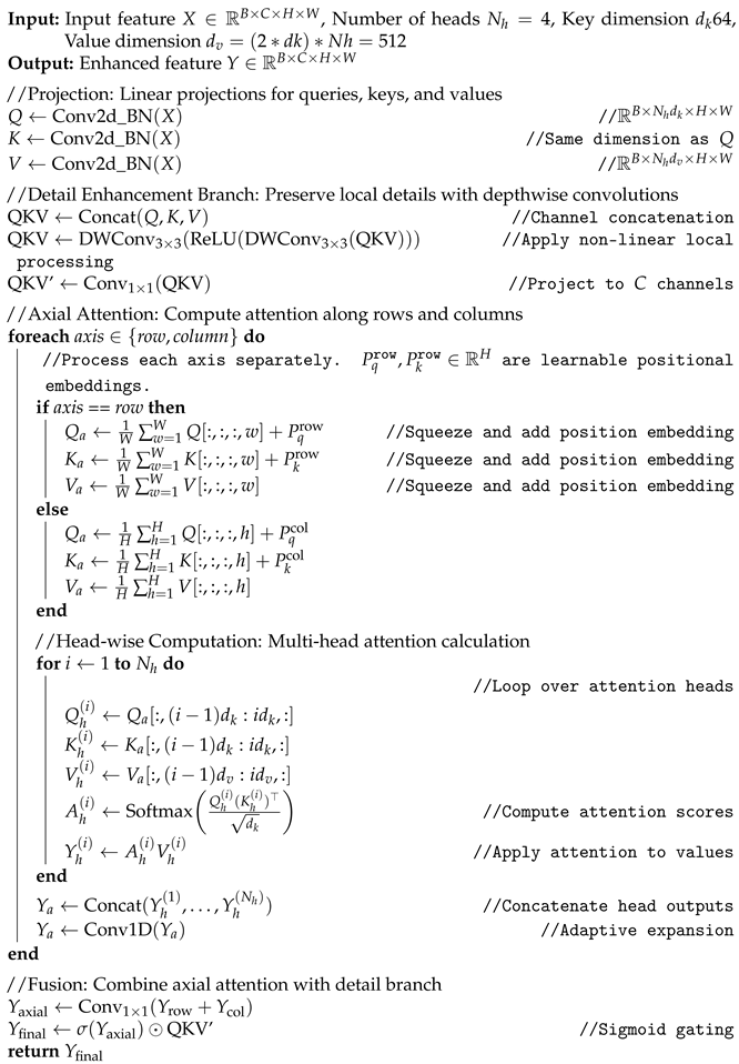
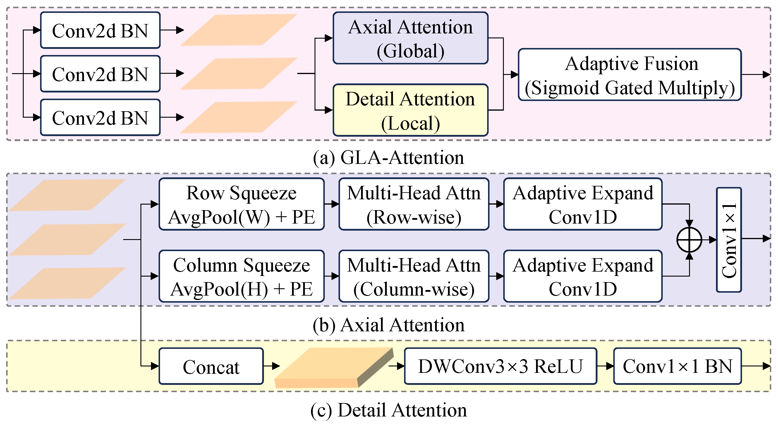
Figure 3.
Architecture of GLA-Attention (a), consisting of an axial attention branch (b) and a detail enhancement branch (c). The squeeze operation reduces spatial dimensions, while positional embeddings capture location-aware features.
Figure 3.
Architecture of GLA-Attention (a), consisting of an axial attention branch (b) and a detail enhancement branch (c). The squeeze operation reduces spatial dimensions, while positional embeddings capture location-aware features.
Figure 4.
Architecture of the proposed C2f-DSLKConv module. (a) The C2f-DSLKConv block splits the input feature map into two parts, processes one through n stacked DSLK-Conv layers, and concatenates the outputs before applying a final convolution. (b) Each DSLK-Conv layer consists of M parallel branches; each branch applies a spatial shift followed by a convolution, with adaptive fusion via a learnable weighting parameter. The weighted branch outputs are summed to yield the final response, enabling efficient large receptive field modeling and flexible feature integration.
Figure 5.
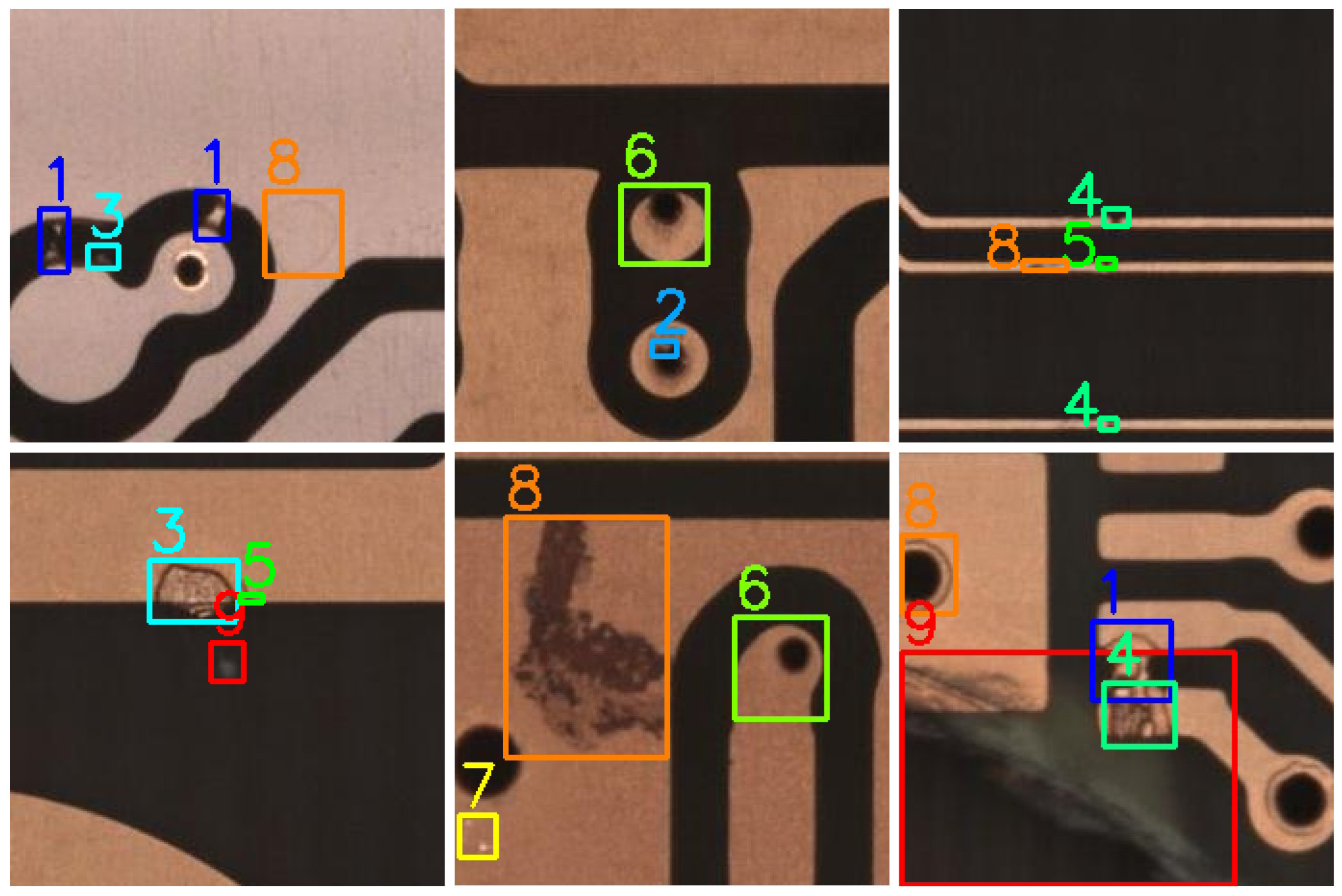
Visual examples of PCB defects.
Figure 5.
Visual examples of PCB defects.
Figure 6.
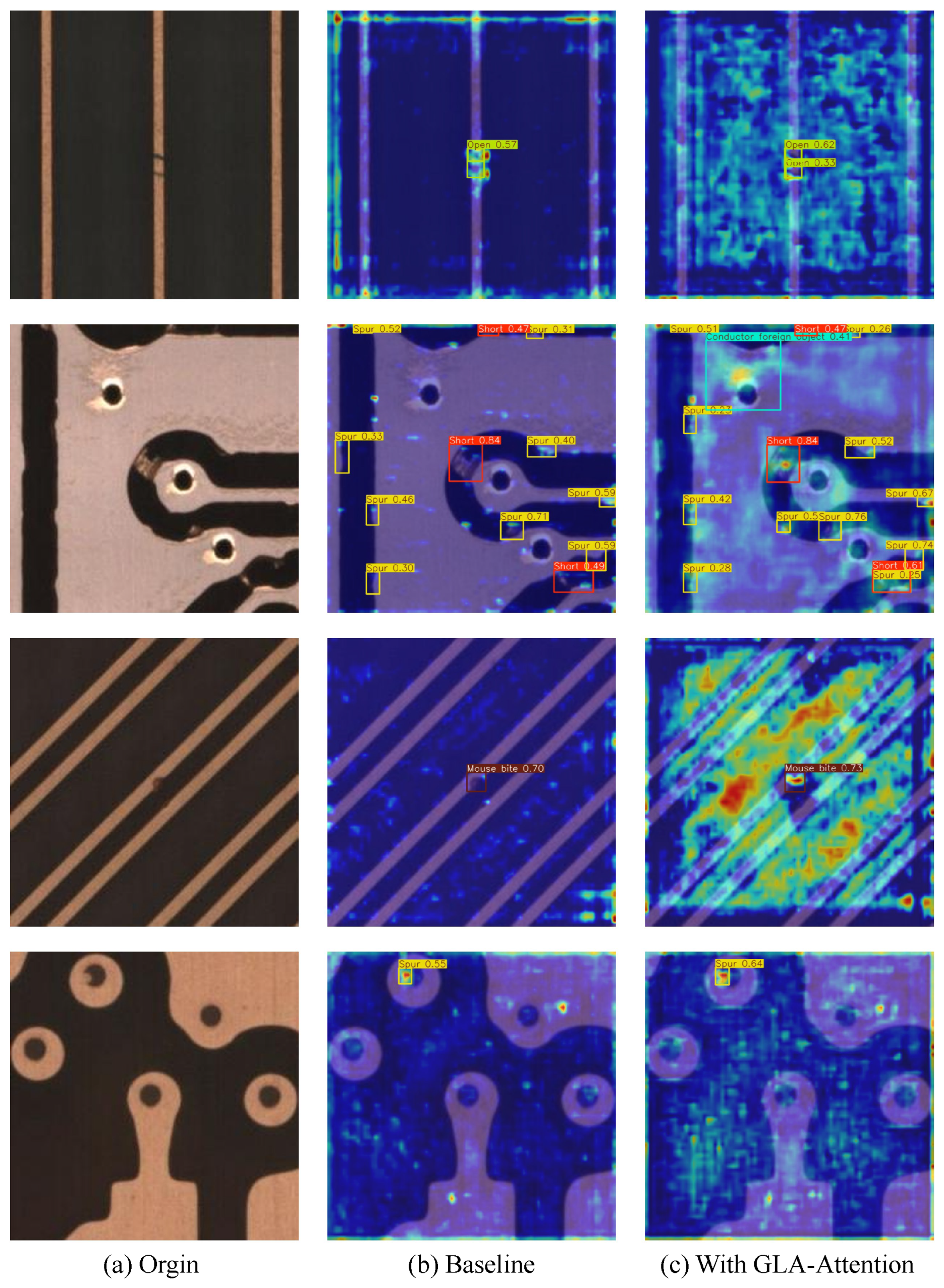
Comparison of attention heatmaps: (a) Original PCB image, (b) Baseline model, (c) Baseline + GLA-Attention. The GLA-Attention module demonstrates more comprehensive global information extraction with broader feature coverage and stronger defect location activation compared to the baseline.
Figure 7.
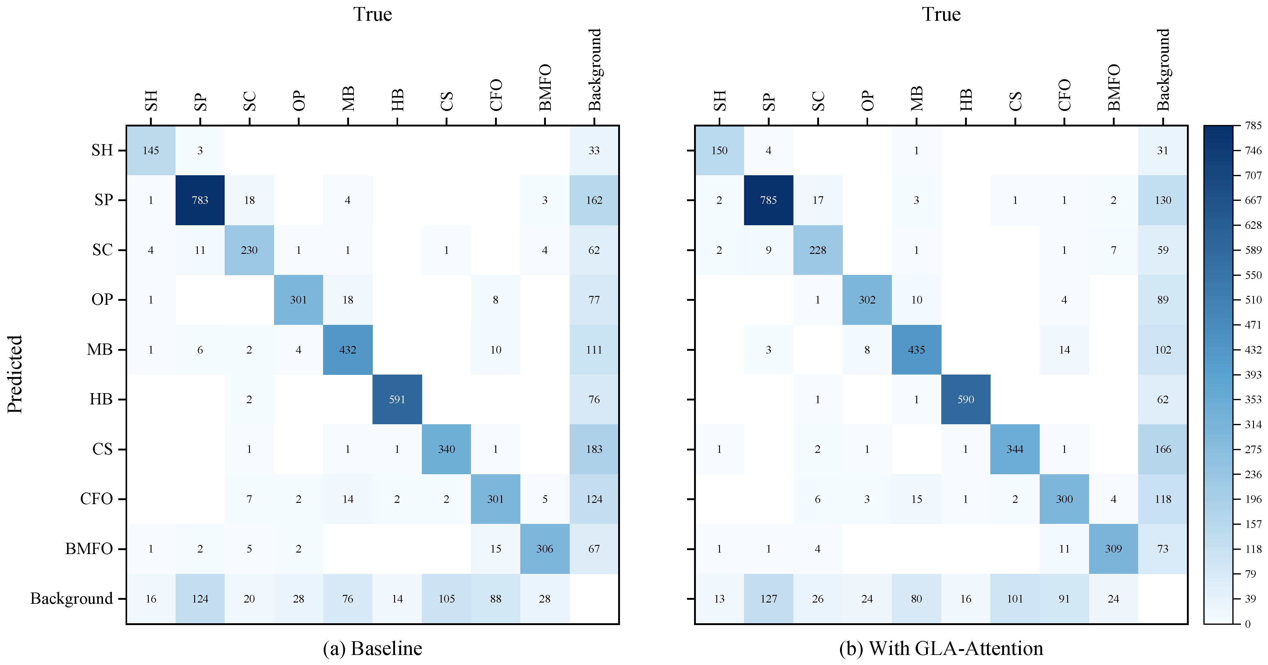
Confusion matrix comparison: (a) Baseline, (b) With GLA-Attention. The GLA-Attention module shows significant improvements in SH, CS, and BMFO categories, demonstrating enhanced capability in extracting both global features for large defects and local features for small defects.
Figure 7.
Confusion matrix comparison: (a) Baseline, (b) With GLA-Attention. The GLA-Attention module shows significant improvements in SH, CS, and BMFO categories, demonstrating enhanced capability in extracting both global features for large defects and local features for small defects.
Figure 8.
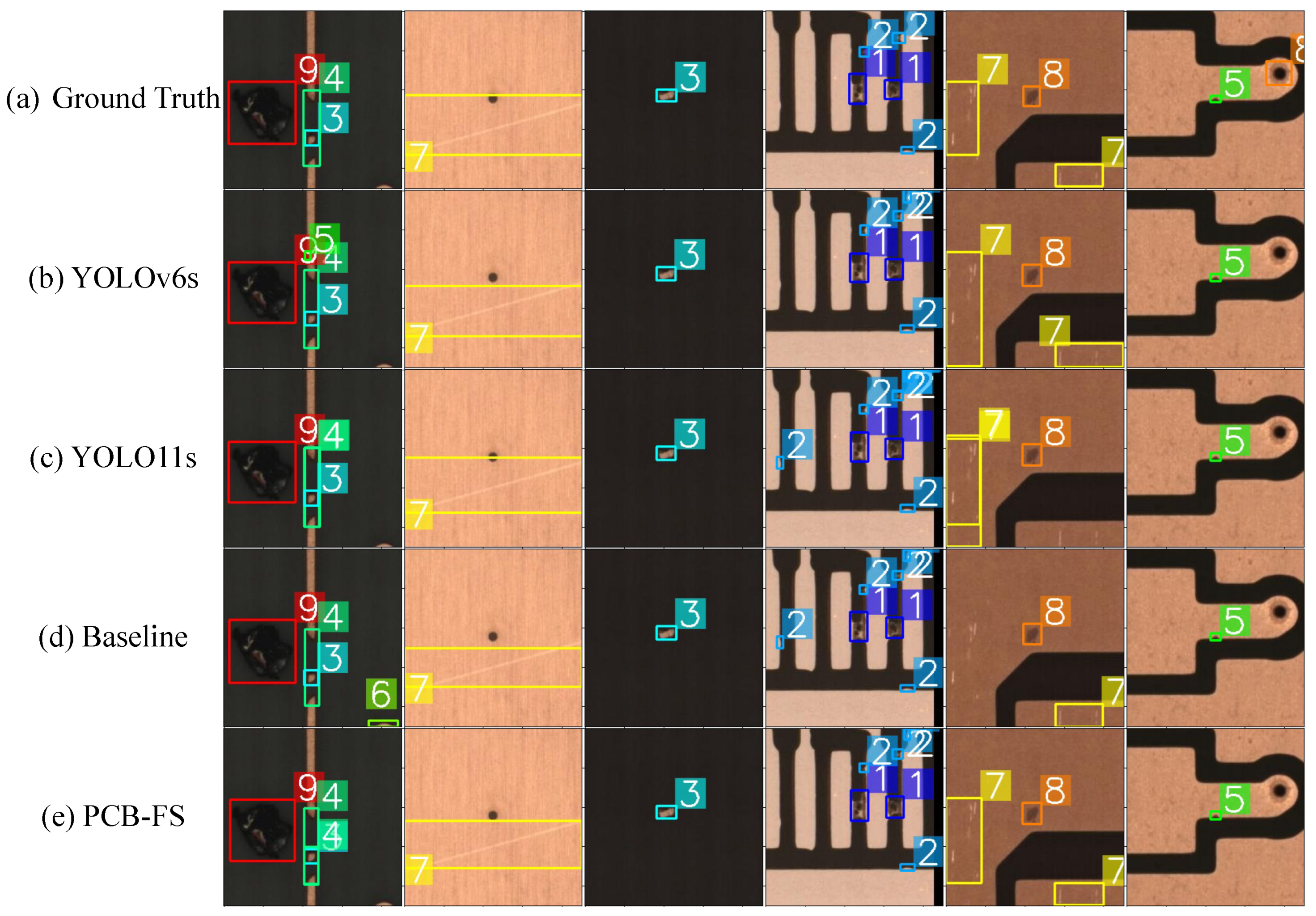
Comparison of defect detection results across different models: Ground truth, YOLOv6s, YOLO11s, Baseline, and PCB-FS.
Figure 8.
Comparison of defect detection results across different models: Ground truth, YOLOv6s, YOLO11s, Baseline, and PCB-FS.
Figure 9.
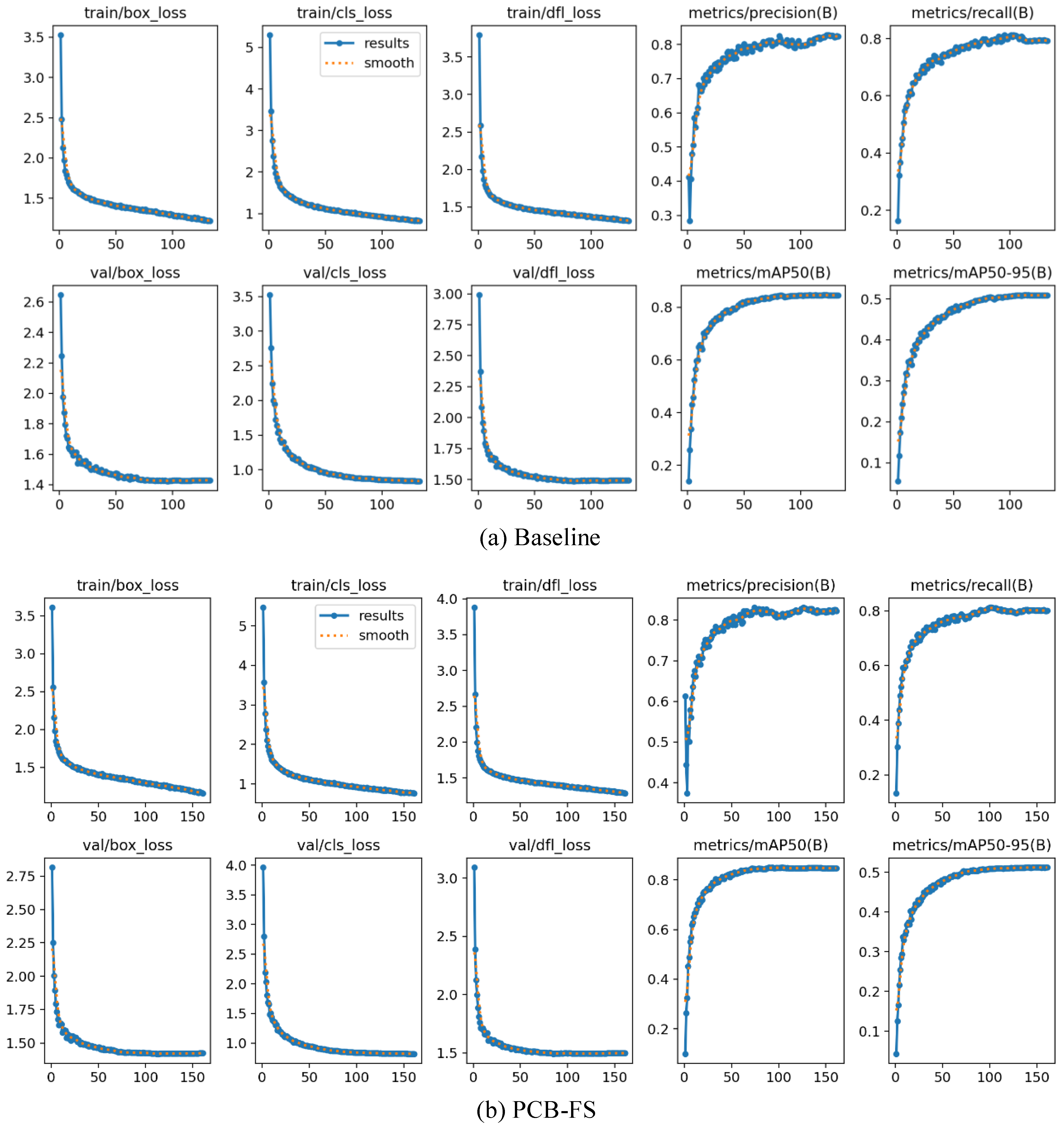
Comparison of training and validation metrics between the baseline and our PCB-FS model. The upper row shows the baseline results, and the lower row shows PCB-FS. From left to right: box loss, classification loss, distribution focal loss, precision, recall, mAP@50, and mAP@50-95. PCB-FS demonstrates faster convergence, lower final loss values, and consistently higher detection performance across all evaluation metrics.
Figure 10.
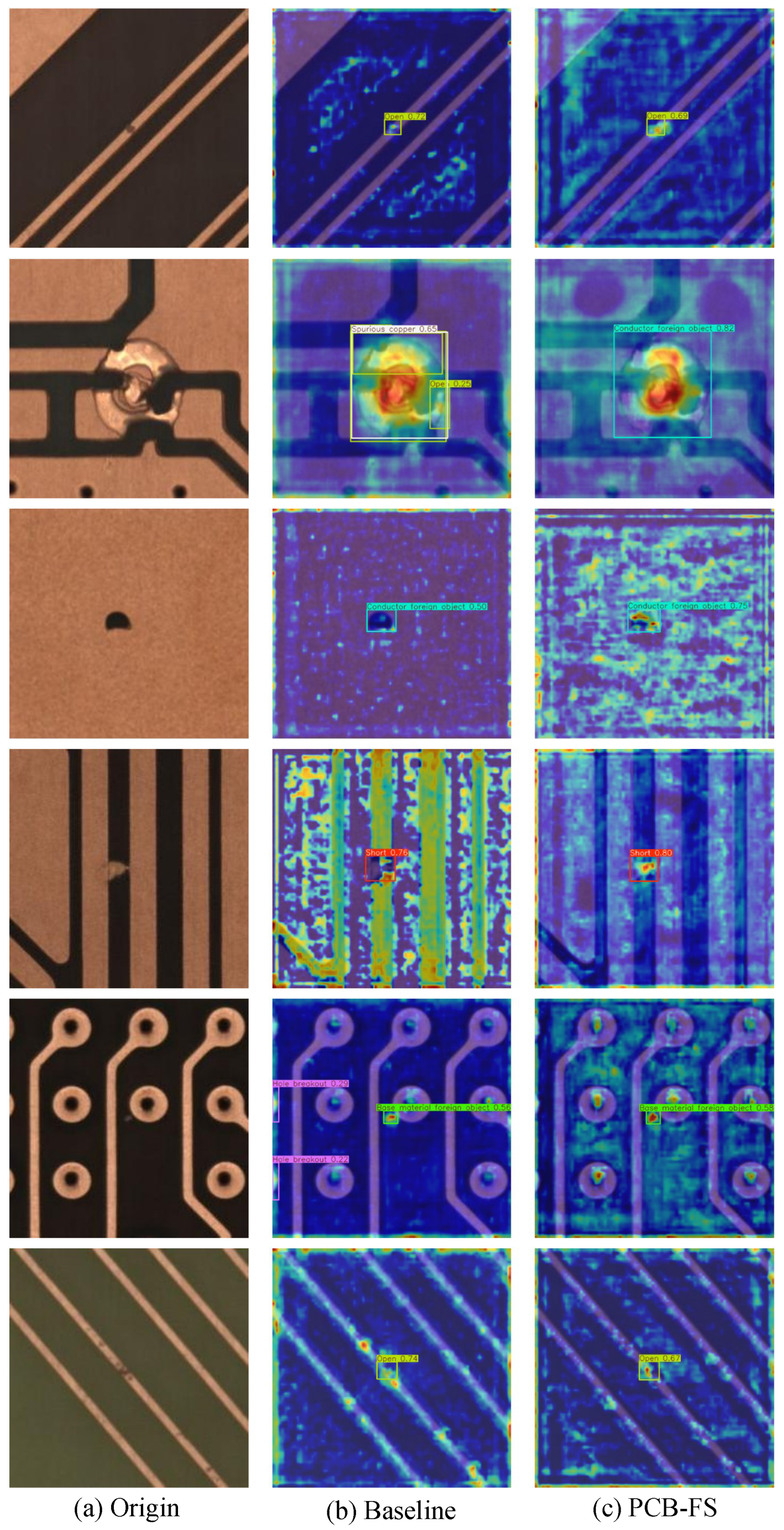
Visualization of defect localization heatmaps. (a) Original PCB image. (b) Baseline model response. (c) Proposed PCB-FS model response. The PCB-FS model produces more accurate and focused activation on true defect regions.
Figure 10.
Visualization of defect localization heatmaps. (a) Original PCB image. (b) Baseline model response. (c) Proposed PCB-FS model response. The PCB-FS model produces more accurate and focused activation on true defect regions.
Figure 11.
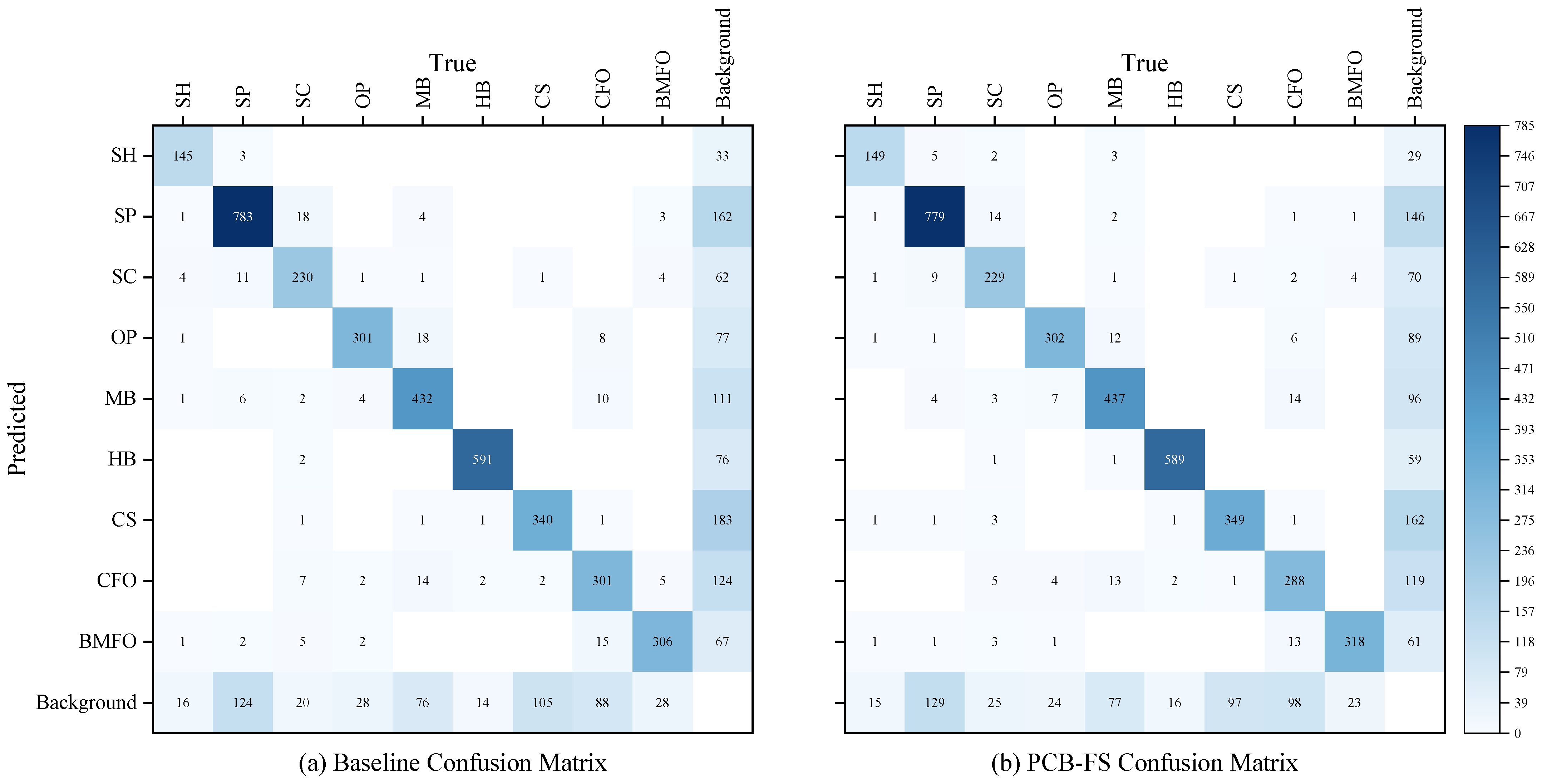
Confusion matrix comparison between the baseline model (a) and our PCB-FS model (b) on the PCB defect detection task. The PCB-FS model achieves higher correct classification rates (diagonal elements) and fewer misclassifications (off-diagonal elements) across all defect categories, demonstrating superior discriminative capability and overall accuracy.
Figure 12.
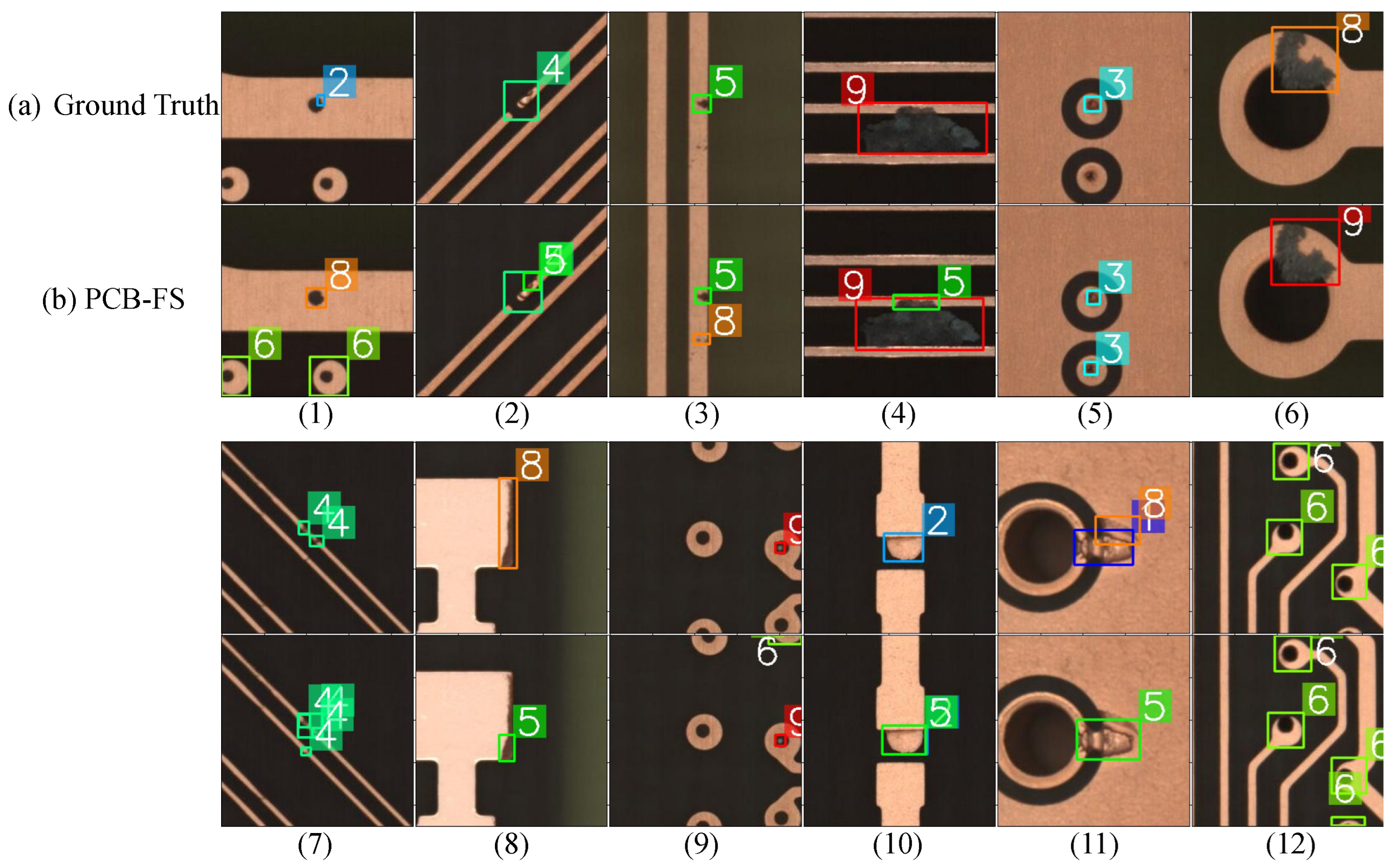
Examples of worst-case detection results: (a) Ground truth, (b) PCB-FS. Numbers 1–12 represent 12 challenging worst-case samples, encoded numerically for reference.
Figure 12.
Examples of worst-case detection results: (a) Ground truth, (b) PCB-FS. Numbers 1–12 represent 12 challenging worst-case samples, encoded numerically for reference.
Table 1.
Computational complexity comparison of different convolution modules. H, W, and C denote the height, width, and number of channels, respectively. K is the number of multi-order FrFT branches.
Table 1.
Computational complexity comparison of different convolution modules. H, W, and C denote the height, width, and number of channels, respectively. K is the number of multi-order FrFT branches.
| Module Type | FLOPs | Params |
|---|
| Standard 3 × 3 Conv | | |
| DD-Conv | | |
Table 2.
Category distribution and scale characteristics of PCB defects.
Table 2.
Category distribution and scale characteristics of PCB defects.
| ID | Color | Defect Type | Defect Size | Train | Test | Total |
|---|
| Small (S) | Medium (M) | Large (L) |
|---|
| 1 | | Short (SH) | 710 | 205 | 0 | 746 | 169 | 915 |
| 2 | | Spur (SP) | 4469 | 115 | 0 | 3655 | 929 | 4584 |
| 3 | | Spurious Copper (SC) | 1352 | 231 | 10 | 1308 | 285 | 1593 |
| 4 | | Open (OP) | 1406 | 361 | 3 | 1432 | 338 | 1770 |
| 5 | | Mouse Bite (MB) | 2421 | 108 | 0 | 1983 | 546 | 2529 |
| 6 | | Hole Breakout (HB) | 35 | 2848 | 0 | 2275 | 608 | 2883 |
| 7 | | Conductor Scratch (CS) | 734 | 1043 | 713 | 2042 | 448 | 2490 |
| 8 | | Conductor Foreign Object (CFO) | 1140 | 582 | 110 | 1409 | 423 | 1832 |
| 9 | | Base Material Foreign Object (BMFO) | 1308 | 304 | 68 | 1344 | 346 | 1680 |
| Total | - | - | 13,575 | 5797 | 904 | 16,184 | 4092 | 20,276 |
Table 3.
Quantitative comparison of PCB defect detection models across performance metrics. Higher values are better for FPS, mAP@50, and mAP@50-95. Best results are highlighted in bold. Confidence intervals (95% CI) from 10 runs.
Table 3.
Quantitative comparison of PCB defect detection models across performance metrics. Higher values are better for FPS, mAP@50, and mAP@50-95. Best results are highlighted in bold. Confidence intervals (95% CI) from 10 runs.
| Model | Backbone | Params (M) | FLOPs (G) | FPS | mAP@50 (%) | mAP@50-95 (%) |
|---|
| DAMOYOLOs [52] | MAE-Res | 15.7 | 36.0 | 34.4 | 84.8 | 48.5 |
| PPYOLOEs [53] | CSRepResNet | 7.9 | 17.3 | 43.2 | 82.7 | 46.0 |
| RTMDETs [54] | CSPDarknet | 8.9 | 14.8 | 38.3 | 84.8 | 48.6 |
| YOLOv5s [15] | C3 | 9.1 | 24.1 | 71.0 | 84.0 | 50.2 |
| YOLOv6s [55] | EfficientRep | 18.5 | 45.2 | 59.3 | 85.2 | 49.7 |
| Rt-DETR [13] | Resnet18 | 20.1 | 60.0 | 35.0 | 85.5 | 51.4 |
| YOLOv10s [56] | CSPDarknet | 8.0 | 24.5 | 47.7 | 84.5 | 51.0 |
| YOLO11s [57] | C3k2 | 9.4 | 21.6 | 73.2 | 85.1 | 51.4 |
| Baseline [58] | CSPDarknet | 10.2 | 24.6 | 110.3 | 84.4 [84.3–84.5] | 51.0 [50.9–51.2] |
| PCB-FS | DSLKConv | 22.3 | 75.8 | 60.8 | 86.2 [86.0–86.3] | 52.4 [52.3–52.4] |
Table 4.
Category-specific detection performance (mAP@50 %) across nine PCB defect types. SH: Short, SP: Spur, SC: Spurious Copper, OP: Open, MB: Mouse Bite, HB: Hole Breakout, CS: Conductor Scratch, CFO: Conductor Foreign Object, BMFO: Base Material Foreign Object. Best results per category are in bold.
| Model | SH (%) | SP (%) | SC (%) | OP (%) | MB (%) | HB (%) | CS (%) | CFO (%) | BMFO (%) |
|---|
| DAMOYOLOs [52] | 91.6 | 83.2 | 83.5 | 91.1 | 82.7 | 97.5 | 72.2 | 74.3 | 87.4 |
| PPYOLOEs [53] | 87.7 | 82.6 | 81.3 | 88.5 | 80.8 | 97.3 | 66.9 | 70.8 | 88.5 |
| RTMDETs [54] | 91.5 | 81.8 | 82.6 | 92.7 | 82.2 | 96.7 | 73.7 | 74.9 | 87.5 |
| YOLOv5s [15] | 89 | 85.4 | 83.5 | 87.7 | 81.2 | 98.5 | 71.1 | 72.1 | 87.5 |
| YOLOv6s [55] | 91.4 | 84 | 83.8 | 91.4 | 83.7 | 97.9 | 73.9 | 72 | 89 |
| Rt-DETR [13] | 93.1 | 85.5 | 84.5 | 91.2 | 83.9 | 97.5 | 73.2 | 73.1 | 87.9 |
| YOLOv10s [56] | 91.1 | 84.6 | 83.1 | 88.2 | 83.3 | 97.7 | 71.9 | 72.2 | 88.5 |
| YOLO11s [57] | 91.4 | 85.4 | 82.7 | 89.7 | 83.6 | 98.4 | 73.8 | 72.4 | 88.1 |
| Baseline [58] | 89.1 | 84.6 | 83 | 89.1 | 82.4 | 98.2 | 72.3 | 73.7 | 87.4 |
| PCB-FS | 91.4 | 86.4 | 84.6 | 91.1 | 84.6 | 98.5 | 75.5 | 73.6 | 90.2 |
Table 5.
We conduct ablation experiments for DD-Conv, GLA-Attention, and C2f-DSLKConv modules using controlled variable methodology. The “×” symbol denotes module exclusion in each experimental configuration.
Table 5.
We conduct ablation experiments for DD-Conv, GLA-Attention, and C2f-DSLKConv modules using controlled variable methodology. The “×” symbol denotes module exclusion in each experimental configuration.
| Baseline | DD-Conv | GLA-Attention | C2f-DSLKConv | mAP@50 | mAP@50-95 |
|---|
| ✓ | × | × | × | 84.4 | 51.0 |
| ✓ | ✓ | × | × | 85.1 | 51.5 |
| ✓ | × | ✓ | × | 85.5 | 52.1 |
| ✓ | × | × | ✓ | 85.1 | 50.8 1 |
| ✓ | ✓ | ✓ | × | 85.9 | 52.2 |
| ✓ | ✓ | ✓ | ✓ | 86.2 | 52.4 |
Table 6.
Comparison of PCB defect detection models on the DeepPCB dataset. The Bold numbers indicate the best performance in each metric.
Table 6.
Comparison of PCB defect detection models on the DeepPCB dataset. The Bold numbers indicate the best performance in each metric.
| Model | Backbone | Params (M) | FLOPs (G) | FPS | mAP@50 (%) | mAP@50-95 (%) |
|---|
| YOLOv5s [15] | C3 | 9.1 | 24.1 | 71.0 | 92.6 | 44.2 |
| YOLOv10s [56] | CSPDarknet | 8.0 | 24.5 | 47.7 | 93.9 | 60.2 |
| YOLO11s [57] | C3k2 | 9.4 | 21.6 | 73.2 | 94.2 | 54.1 |
| Baseline [58] | CSPDarknet | 10.2 | 24.6 | 110.3 | 93.3 | 51.9 |
| PCB-FS | DSLKConv | 22.3 | 75.8 | 60.8 | 96.0 | 63.2 |
