Article

Automatic Segmentation of Temporomandibular Joint Components Using Asymmetric Kernels in a DenseUNet Architecture

by
Edgar F. Duque-Vazquez
1,
Ivan Cruz-Aceves
2,
Raul E. Sanchez-Yanez
3 and
Jonathan Cepeda-Negrete
1,*
1
División de Ciencias de la Vida (DICIVA), Universidad de Guanajuato, Campus Irapuato-Salamanca, Carretera Irapuato-Silao km 9 ap 311, Irapuato 36500, Mexico
2
Centro de Investigación en Matemáticas (CIMAT), A.C., Secretaría de Ciencia, Humanidades, Tecnología e Innovación (SECIHTI), Jalisco S/N, Col. Valenciana, Valenciana 36023, Mexico
3
División de Ingenierías (DICIS), Universidad de Guanajuato, Campus Irapuato-Salamanca, Carretera Salamanca-Valle de Santiago km 3.5 + 1.8 Comunidad de Palo Blanco, Salamanca 36885, Mexico
*
Author to whom correspondence should be addressed.
Symmetry 2025, 17(12), 2014; https://doi.org/10.3390/sym17122014
Submission received: 10 October 2025 / Revised: 12 November 2025 / Accepted: 14 November 2025 / Published: 21 November 2025

Abstract

Accurate evaluation of the Temporomandibular joint (TMJ) components is essential for proper diagnosis and treatment. However, the current diagnostic process relies heavily on manual measurements, which are time-consuming and prone to human error. Here, the fundamental task is performed using imaging techniques and locating regions of interest in the TMJ. Nowadays, such image segmentation has been automated using a number of deep learning models. Nonetheless, developed models for TMJ segmentation are primarily built on symmetric convolutional kernels, which may limit their ability to capture the inherently asymmetric structures of the joint. To address this gap, this work proposes a novel approach that integrates an asymmetric kernel into a DenseUNet architecture and squeeze-and-excitation blocks for the automatic segmentation of three key morphological components of the TMJ. A metaheuristic iterated local search algorithm was used to identify the most effective kernel configuration within a search space of 15 2 asymmetric kernel combinations. The resulting optimized architecture was trained and evaluated on a TMJ imaging dataset and compared against nine state-of-the-art segmentation architectures. The proposed method achieved the highest Dice coefficient of 0.78, outperforming all baseline architectures, and demonstrated efficient processing with an average inference time of 0.16 s per image. These results highlight the potential of the proposed system to enhance the accuracy and efficiency of TMJ diagnostics in clinical settings.

1. Introduction

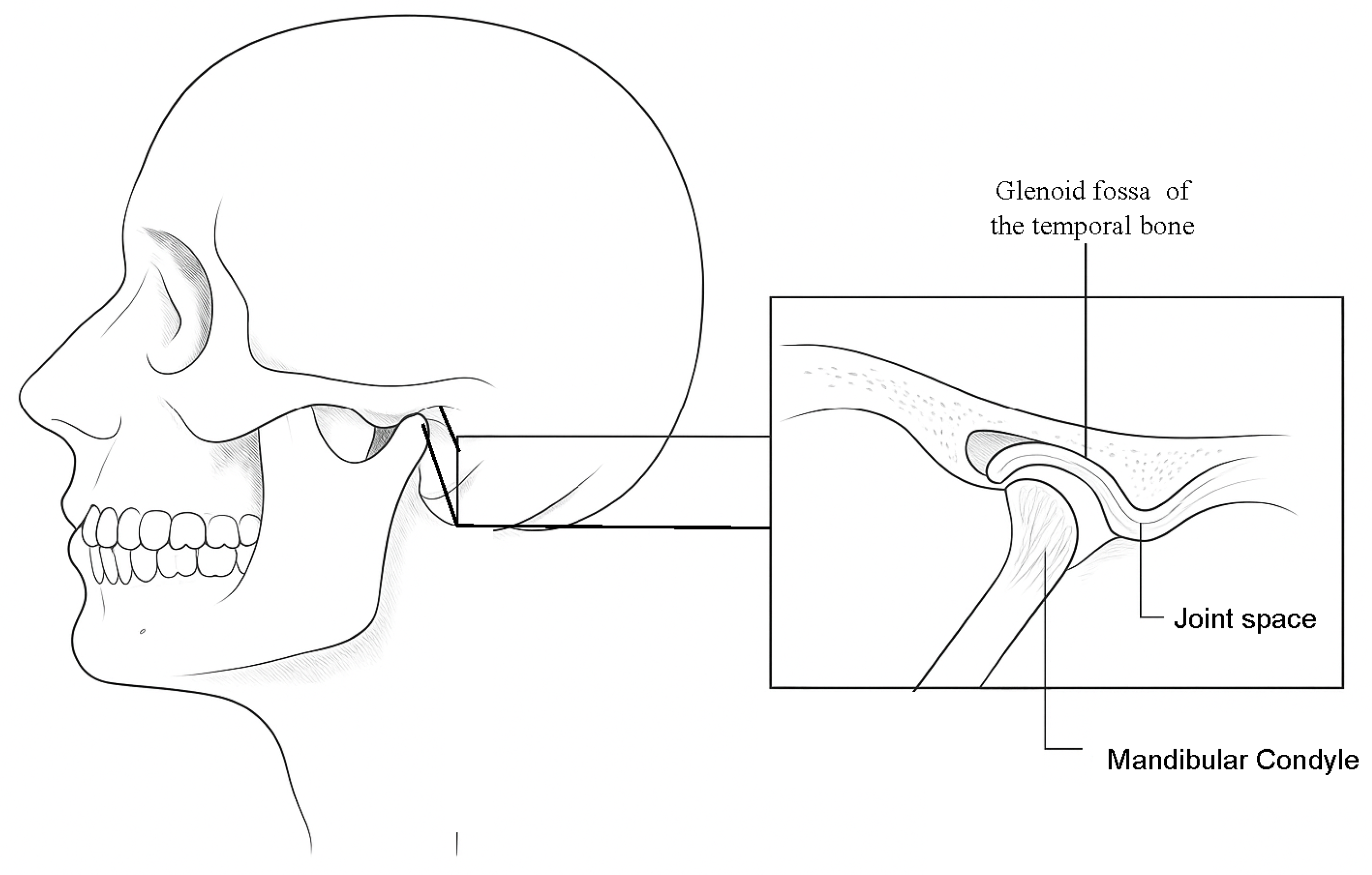
The articulatory system consists of the temporomandibular joint (TMJ), intra-articular discs, jaw muscles, and occlusion. The TMJ, which connects the upper and lower jaws [1], is a paired and symmetrical joint, whose coordinated functionality on both sides of the mandible is essential for balanced jaw movement. The superior compartment separates the glenoid fossa of the temporal bone from the disc, while the inferior compartment separates the disk from the mandibular condyle (see Figure 1). This bilateral and symmetric arrangement enables speech, chewing, and both verbal and emotional expression [2]. Temporomandibular disorders (TMD) are conditions that affect the temporomandibular joint and associated structures. Even though the TMJs are structurally symmetrical, pathology often leads to functional asymmetry, producing alterations in disk positioning, joint space, and condylar mobility. These imbalances may arise from any stimulus impacting a component of the articulatory system, potentially influencing the entire system. The most common disorders include disk alterations, joint pain, joint dysfunction, and degenerative joint disease [3]. TMDs are among the most prevalent pathologies, with a higher incidence in the Americas [4], and primarily affect women [5]. The pain associated with TMD is often comparable in intensity and persistence to cervical pain, back pain, and headaches, significantly impacting the quality of life of patients. Consequently, the observation and assessment of the TMJ have become essential in the orofacial field.
One approach for evaluating the TMJ involves measuring the joint space width through imaging techniques, with particular attention on detecting reductions. In this approach, it is essential to highlight components, such as the mandibular condyle, joint space, and the glenoid fossa of the temporal bone. Imaging techniques employed in the examination of the TMJ include computed tomography (CT), cone beam computed tomography (CBCT), and magnetic resonance imaging (MRI), with the latter being the most frequently utilized for evaluating intra-articular processes [7]. These techniques yield static images, which present a significant limitation in evaluating the dynamic movements of the TMJ, especially during real-time assessments. To address this limitation, ultrasonography offers an alternative approach, as it is both readily accessible and cost-effective for evaluating the TMJ [2]. Despite the advancements offered by ultrasonography, evaluation of the TMJ continues to rely on manual measurements, inherently prone to errors and, sometimes, time-consimung. Consequently, there is a growing interest in exploring alternative approaches to automate these processes and improve diagnostic precision in TMJ assessments. Artificial intelligence has proven to be an effective tool for optimizing this process. In biomedical imaging, deep learning has made significant progress, allowing models to handle tasks such as classification, detection, tracking, and segmentation [8].
Several studies have applied deep learning techniques to the segmentation of TMJ components. Most of these works focus on MRI images [9], leveraging their high resolution and ability to visualize soft tissues. For instance, Ito et al. [10] developed 3DiscNet for the automated detection and segmentation of the TMJ disc, and evaluated their architecture with two architectures: U-Net, and SegNet. The highest Dice coefficients achieved by 3DiscNet and SegNet were 0.70 and 0.74, respectively. Similarly, Kin et al. [11] proposed a deep learning-based algorithm to predict TMJ disk perforation, employing a multilayer perceptron and comparing it with a Random Forest model. In their work, the multilayer perceptron achieved the highest performance, with an Area Under the Curve (AUC) of 0.94. Additionally, Li et al. [12] utilized convolutional neural networks to delineate the mandibular condyle, articular eminence, and TMJ disc. A Dice coefficient of approximately 0.7 was obtained for the articular disc, while values greater than 0.9 were achieved for the mandibular condyle. Beyond MRI, some studies have explored CBCT images for TMJ analysis. Mao et al. [13] developed an automated system for diagnosing degenerative TMJ disease using a YOLOv10-based algorithm. Choi et al. [14] evaluated multiple architectures, Res18, Res50, Res101, VGG16, VGG19, and GoogleNet, to diagnose joint disease, with GoogleNet yielding the F1-score of 0.72. However, these studies do not involve ultrasound imaging for the TMJ, and research utilizing ultrasound in this context remains scarce. Currently, the only study reported is that of Lasek et al. [4], upon which the current work is based.
Lasek et al. proposed and validated an artificial intelligence-driven approach for the automatic and consistent measurement of TMJ space width using ultrasound imaging. Their methodology encompassed the evaluation of seven deep learning architectures: Attention U-Net, U-Net++, DeepLabv3, SegResNet, SegResNet with a Variational Autoencoder, Residual U-Net, and V-Net. The goal was to segment three key TMJ structures: the mandibular condyle, the joint space, and the glenoid fossa of the temporal bone. Among the models assessed, Residual U-Net exhibited the highest performance, reaching a Dice coefficient of 0.75. These findings underscore the complexity of accurately segmenting TMJ components in ultrasound images and reflect the persistent challenges associated with this task [4], and the need for improved models capable of enhancing segmentation accuracy.
Recent studies have explored the challenge of detecting weak or asymmetric features in medical images using attention and feature fusion mechanisms. For instance, Rehman et al. [15], proposed a hybrid Vision Transformer (ViT) and VGG-16 framework to detect architectural distortions in mammograms, effectively addressing texture heterogeneity and subtle structural asymmetries. Similarly, Pan et al. [16], introduced YOLO-TARC, a YOLOv10 variant with token attention and residual convolution, achieving superior detection of small voids in dental X-ray images. These approaches highlight the relevance of attention-based and adaptive kernel mechanisms for enhancing the representation of subtle anatomical patterns an aspect also crucial for accurate TMJ ultrasound segmentation.
Inspired by the scarce exploration of TMJ segmentation using ultrasound imaging, this work introduces a novel DenseUNet architecture. The model integrates optimized asymmetric convolutional kernels via an iterated local search metaheuristic to better capture directional texture variations, a characteristic of ultrasound data. Unlike approaches that rely on fixed symmetric kernels (e.g., 3 × 3 ), our method introduces an automatic optimization strategy to adapt kernel shapes for ultrasound data. This allows the model to more effectively capture directional and elongated texture variations, which are characteristic of this imaging modality. Additionally, Squeeze-and-Excitation blocks are incorporated to enhance feature recalibration and improve representational capacity. The proposed approach achieved a Dice coefficient of 0.78 and an average processing time of 0.16 s per image, outperforming twelve architectures and demonstrating its capacity to advance the automatic analysis of TMJ structures in ultrasound images.
The remainder of this paper is organized as follows. Section 2 details the dataset and outlines the methodologies employed in the proposed architecture. Section 3 presents the experimental results and provides a comprehensive discussion, supported by illustrative images and graphs to aid interpretation. Lastly, the paper concludes with a summary of the principal findings.

2. Materials and Methods

This section outlines the materials and methods utilized in the study. It begins by describing the dataset used for training and performing an evaluation of the segmentation models that were implemented. Subsequently, the DenseNet and DenseUNet architectures are introduced to provide context for the proposed method. Finally, the iterated local search algorithm is presented as a core element of the experimental framework.

2.1. Dataset of Temporomandibular Joint Components

The “Ultrasound Images of the Temporomandibular Joint with Segmentations” dataset [17], used to train and validate the proposed architecture, originates from the study by Lasek et al. [4]. It comprises ultrasonographic assessments of the TMJ, captured using morphological imaging slices aligned, parallel to the joint line. This dataset, which is available for downloading from the authors upon request, includes 142 images, each paired with its corresponding ground-truth annotation. The images have a resolution of 580 × 740 pixels and are stored in an 8-bit grayscale format. Data acquisition was performed using a GE HealthCare ultrasound system at the Department of Radiology and Ultragen Medical Clinic in Poland. Figure 2a shows examples of visual representations of the dataset, displaying both the raw ultrasound images and their corresponding three-class ground-truth.
The dataset is annotated into three classes, each corresponding to an anatomically relevant component of the TMJ: the mandibular condyle (MC), which forms the inferior portion of the joint; the joint space (JS); and the glenoid fossa of the temporal bone (GF), which constitutes the superior aspect of the TMJ. Initially, segmentation was performed automatically using a UNet model. The results were then manually refined by a radiologist to ensure annotation accuracy. Figure 2 illustrates these classes, with Figure 2b showing examples of the MC, Figure 2c depicting the JS, and Figure 2d presenting the GF.

2.2. DenseNet and DenseUNet

A deep neural network is a computational model made of multiple layers of multiple interconnected processing units. These networks exhibit the ability to discriminate patterns after providing numerous samples to learn from. A number of such structures, also known as deep learning models, have been proposed for image analysis, being particularly successfully for the image segmentation task. Deep learning models for image analysis have evolved by incorporating mechanisms that improve feature propagation and reuse across layers. One of the most influential approaches in this regard is the Densely Connected Convolutional Network (DenseNet), proposed by Huang et al. [18]. While DenseNet focuses on enhancing general-purpose CNNs, U-Net [19] was specifically designed for biomedical image segmentation. DenseUNet, introduced by Cao et al. [20], merges the advantages of both architectures. Distinctive contribution of DenseUNet lies in the use of dense blocks, where each layer receives as input the concatenated outputs of all preceding layers. This strategy not only enriches the representational capacity of the network but also alleviates the vanishing gradient that affects learning algorithms. Formally, if x 0 denotes the input image, the output of the lth layer is defined as:
x l = H l ( [ x 0 , x 1 , , x l 1 ] ) ,
where H l is a composite transformation consisting of operations such as batch normalization, ReLU, pooling, or convolution. Within each dense block, the standard sequence of operations is batch normalization, followed by ReLU activation, and then a 3 × 3 convolution. To regulate the dimensionality of feature maps, transition layers, including convolution and pooling, are inserted between dense blocks. The encoder–decoder design allows the extraction of hierarchical features while progressively reconstructing fine-grained spatial details. Skip connections bridge the encoder and decoder, ensuring the preservation of spatial information that would otherwise be lost during downsampling. Owing to its versatility, U-Net has been successfully applied to a wide range of medical tasks, including brain imaging, vessel segmentation, and cell nuclei analysis [21].
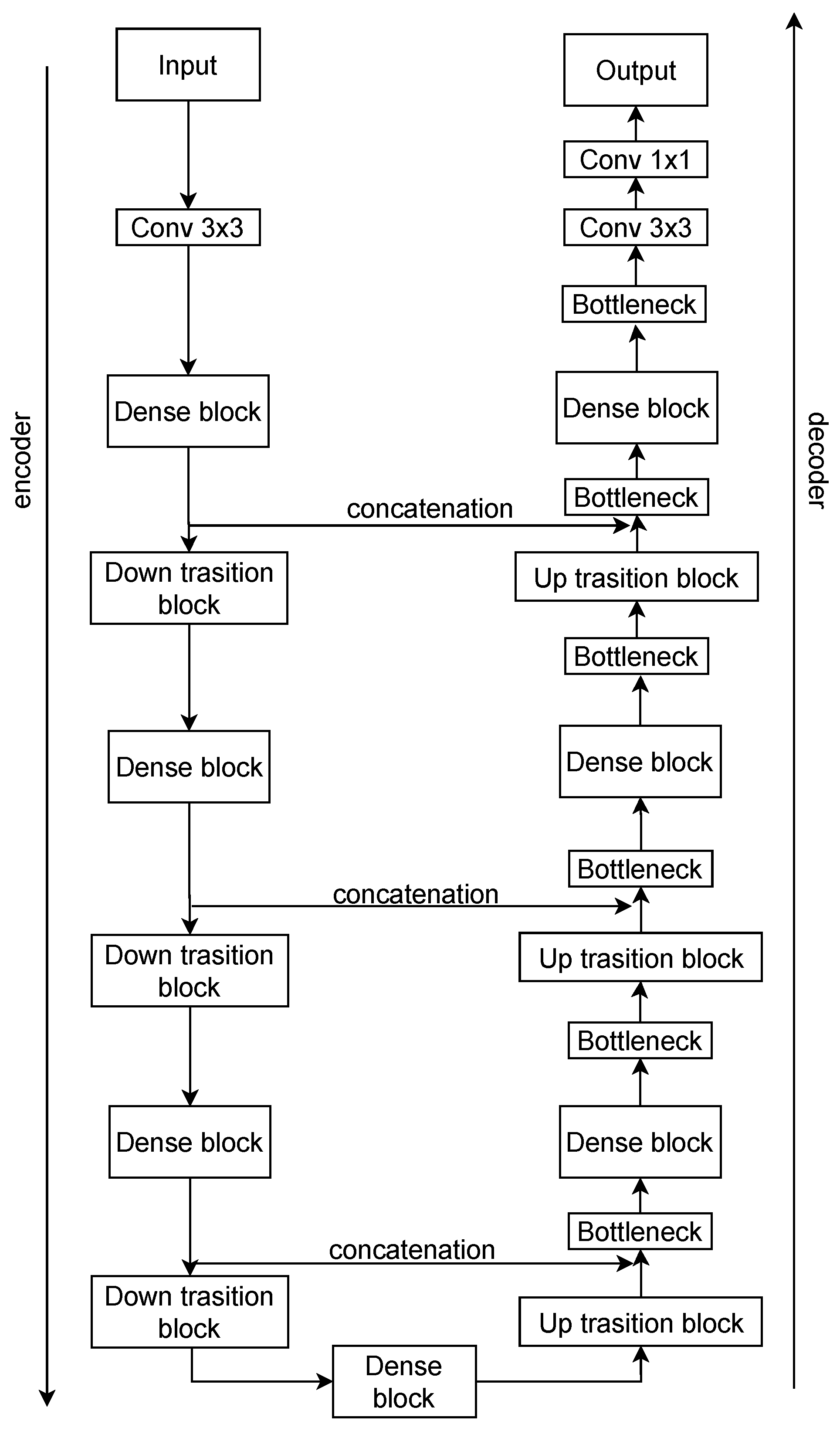
DenseUNet extends U-Net by embedding dense connectivity within its core building blocks, enabling more efficient feature reuse and robust gradient flow. Its design is structured around four key components: Down Transition blocks, Up Transition blocks, Dense Blocks, and a Bottleneck (Figure 3). The contracting path applies successive Down Transition blocks each composed of a 2 × 2 max pooling layer (stride 2) and dropout (rate 0.2), which halve the spatial resolution while increasing the number of channels. Symmetrically, the expanding path restores spatial resolution via Up Transition blocks, where upsampling and dropout (rate 0.2) are followed by concatenation with encoder features through skip connections.
A bottleneck layer, consisting of a 1 × 1 convolution and dropout, is applied before and after the dense blocks to limit computational complexity. Finally, the segmentation map is produced by a 3 × 3 convolution, followed by a 1 × 1 convolution and a sigmoid activation. This architecture achieves a balanced integration of spatial preservation of the U-Net and feature aggregation of the DenseNet, making DenseUNet highly suitable for biomedical segmentation tasks.

2.3. Iterated Local Search

In the proposed work, Iterated Local Search (ILS) serves as a key optimization mechanism for determining optimal sizes of asymmetric convolutional kernels. ILS belongs to the family of meta-heuristic algorithms and builds upon local search methods by introducing perturbations that allow the exploration of new regions in the solution space [22,23]. Its strength lies in balancing intensification (via local refinement) and diversification (through perturbations), making it highly effective for combinatorial and discrete optimization problems that contain numerous local optima. Unlike plain local search, which often stagnates, ILS can escape local minimal and maintain a steady improvement trajectory. Its modular structure, ease of implementation, and low computational cost make it attractive for challenging optimization tasks such as kernel design in deep learning [24].
An ILS process is typically structured around four components: the creation of an initial solution, a local search phase to improve it, a perturbation step that modifies the current solution to explore alternative configurations, and an acceptance criterion that determines whether the new solution replaces the previous one. The algorithm begins with a randomly generated solution, which is iteratively refined by alternating local optimization and perturbation, thus ensuring both exploration and exploitation of the search space [25]. The basic procedure is described in Algorithm 1.
Algorithm 1: Iterated Local Search
  1:
Input: Stopping criterion S
  2:
Output: Best solution x *
  3:
Initialize solution x 0 randomly
  4:
while S is not satisfied do
  5:
     x = LocalSearch ( x )
  6:
     x = Perturb ( x )
  7:
     x * = LocalSearch ( x )
  8:
end while
The iterative cycle of search and perturbation makes ILS particularly suitable for optimization problems with vast and complex landscapes. In this work, each solution encodes a specific arrangement of asymmetric convolutional kernels. The process starts with the random selection of kernel dimensions. During perturbation, either the width or height of one or more kernels is modified, while the subsequent local search step fine-tunes the resulting configuration by examining nearby alternatives. The objective function guiding this optimization is the Dice coefficient, computed over the validation dataset, ensuring that the best-performing kernel configuration is progressively identified.

3. Proposed DenseUNet with Asymmetric Kernels

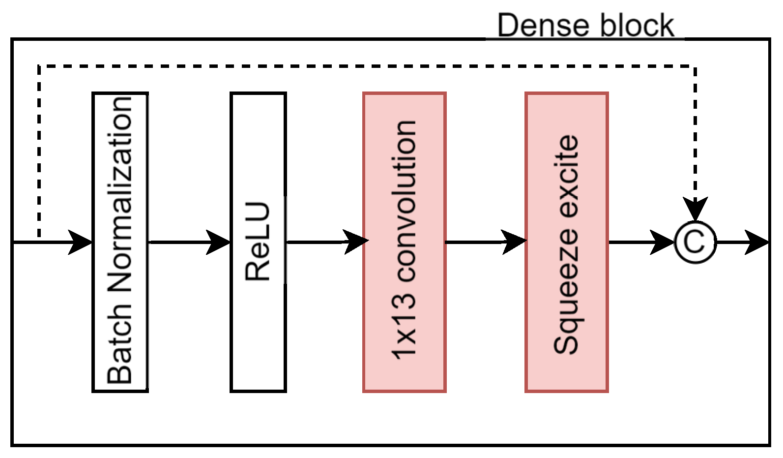
DenseUNet architecture was modified with two main improvements. First, the kernel sizes within the dense blocks were adjusted using ILS to generate a optimized asymmetric kernel, which enhance the capability of the model to capture elongated structures. Second, a squeeze-and-excitation (SE) block was integrated into each dense block, allowing the network to better model inter-channel dependencies. The following sections describe these changes in detail, and Figure 4 illustrates the modified dense block, with the alterations highlighted in red.
Each dense block is composed of l layers, where each layer applies a non-linear transformation H l ( · ) . In this work, H l ( · ) is defined using 1 × 13 and 13 × 1 convolutional filters, followed by a ReLU activation and an SE block (see Figure 4). The convolutional kernels alternate between 1 × 13 and 13 × 1 depending on whether the layer index l is even or odd. This design enables directional feature extraction in both vertical and horizontal orientations, thereby introducing asymmetry into the convolutions.
The kernel dimensions were optimized using an ILS algorithm, aiming to identify the most effective asymmetric configurations ( 1 × 13 and 13 × 1 ). The optimization objective was to maximize the segmentation accuracy, measured by the Dice coefficient on the validation set. The search process consisted of 150 iterations, exploring kernel sizes between 1 and 15, which resulted in a search space of 15 2 possible configurations. At each iteration, a candidate configuration was evaluated, and the best-performing solution was retained. The neighborhood of a solution was defined by varying one kernel dimension (x or y) by ±1 while keeping the other fixed. If no improvement in the Dice coefficient was observed after a local search, a perturbation was applied by randomly modifying one of the kernel dimensions of a convolutional filter ( x × y ) to escape local optima. A new configuration was accepted only if it achieved a higher Dice score than the current best. The search terminated when no improvement was observed over five consecutive iterations or when the iteration limit (150) was reached.
The SE block recalibrates the convolutional feature maps [26] through three phases: squeeze, excitation, and rescaling. During the squeeze step, global average pooling reduces the spatial dimension of each feature map, generating a channel descriptor. Next, in the excitation step, two fully connected layers with ReLU and sigmoid activation are used to model non-linear inter-channel dependencies. Finally, in the rescaling phase, the learned channel weights are applied to the original features, highlighting the most informative channels and suppressing less relevant ones.
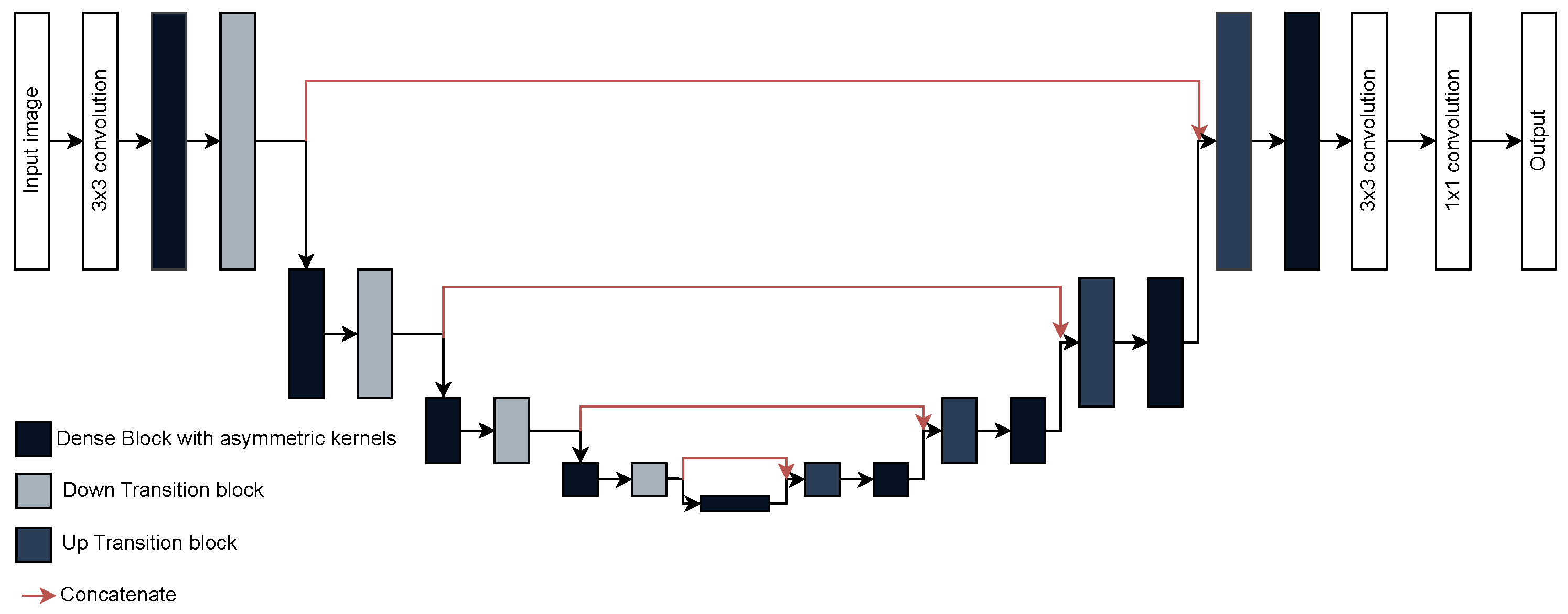
The proposed model preserves the overall organization of the DenseUNet introduced by Cao et al. [20] (Figure 5), consisting of three stages: encoder, bridge, and decoder. The encoder is built from a sequence of dense blocks followed by transition layers, repeated four times to extract progressively deeper features. The bridge contains an additional dense block that encodes abstract global representations. The decoder mirrors the encoder structure, with up-sampling layers followed by dense blocks, also repeated four times, to gradually refine the segmentation output. Each dense block was set to include four layers with a growth rate of 16, determining the number of feature maps produced per layer. The network was trained using 75% of the images for training and the remaining 25% was used for validation and testing. It is important to mention that the dataset was already organized into predefined subfolders, so a random split was not required. Training was performed for 30 epochs with a batch size of 4, using categorical cross-entropy as the loss function. The model was optimized with the Adam optimizer using its default parameters (learning rate = 0.001, β 1 = 0.9, β 2 = 0.999, ϵ = 1 × 10 7 ). To ensure reproducibility, all experiments were conducted with fixed random seeds across NumPy, TensorFlow, and Python environments.
To evaluate the performance of the proposed model, standard segmentation metrics were employed and compared with existing approaches [4]. The chosen metrics were the Dice coefficient, Precision, Recall, and F1-score all of which compare the predicted segmentation to the ground-truth. These metrics take values between 0 and 1, where higher values indicate greater similarity. For this work, assuming that the target class is assigned the label value 1 among the four possible class labels (0: background, 1: MC, 2: JS, and 3: GF), true positives (TP) correspond to pixels correctly predicted as class 1. False positives (FP) are pixels incorrectly predicted as class 1 but actually belonging to classes 0, 2, or 3. False negatives (FN) refer to pixels from class 1 that were incorrectly labeled as 0, 2, or 3. The definitions of the metrics are as follows in Equations (2)–(5):
D i c e = 2 T P 2 T P + F P + F N
P r e c i s i o n = T P T P + F P
R e c a l l = T P T P + F N
F 1 s c o r e = 2 × precision × Recall Precision + recall

4. Results and Discussion

This section presents the results obtained from the experiments. First, the results of the ILS algorithm are discussed, analyzing the impact of kernel size selection on the Dice coefficient and computation time. Next, the performance of the proposed DenseUNet model is evaluated by comparing it with reference architectures. A quantitative analysis is provided to illustrate the strengths and limitations of the proposed approach. Finally, a visual analysis is presented to examine the segmentation results from a qualitative perspective.
The experiments presented in this section were conducted using the servers of Laboratorio de Supercómputo del Bajío (Lab-SB), with the following specifications: 128 GB of RAM, an Intel Xeon Silver 4214 processor, and an NVIDIA Titan RTX 24 GB graphics card. All implementations were developed in Python 3.10.12, utilizing TensorFlow 2.1.0.
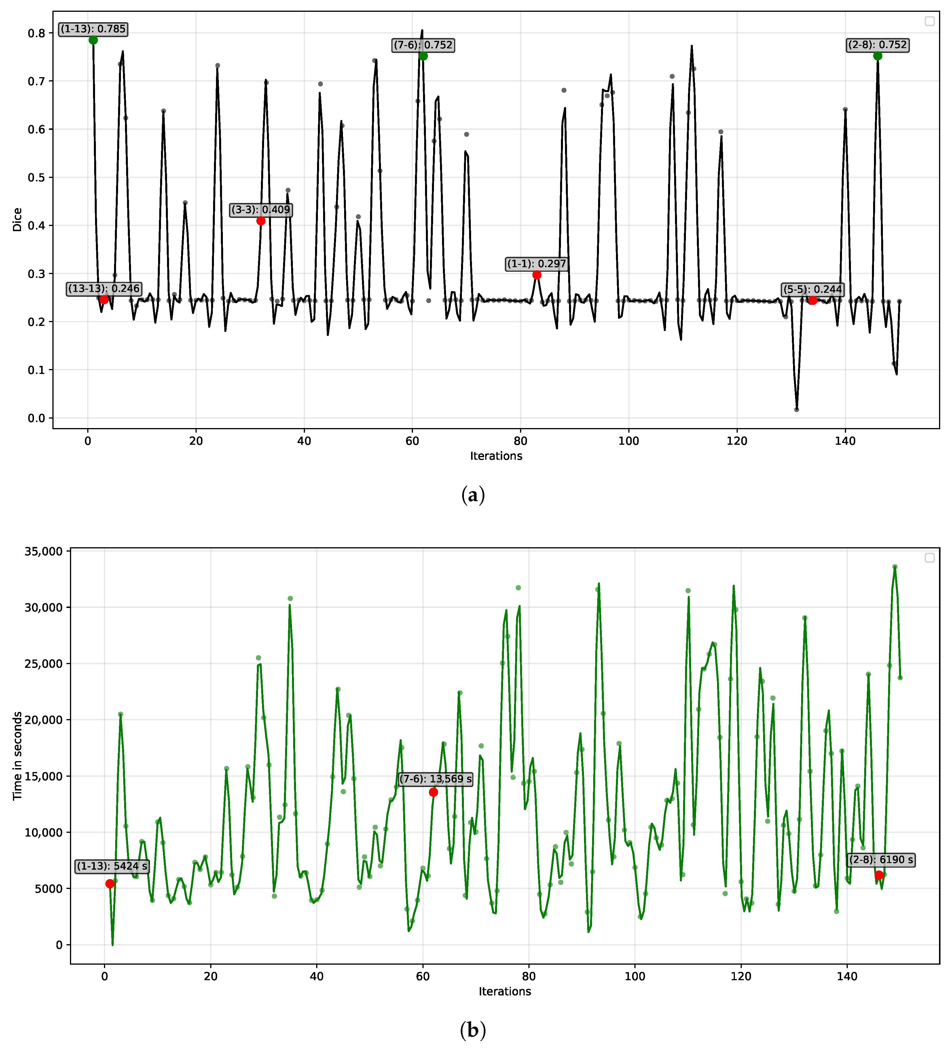
The proposed architectural improvements were specifically applied to the dense block of DenseUNet, including kernel size adjustments and the integration of an SE block. To identify the optimal configuration of the asymmetric kernel, a search was performed using the ILS algorithm. Figure 6a depicts the evolution of filter combinations across 150 iterations. The y-axis represents the iteration number, while the x-axis corresponds to performance, measured by the Dice coefficient (ranging from 0 for low performance to 1 for high performance). Each model was trained for 30 epochs under identical hyperparameters, with kernel size as the only varying factor.
The ILS algorithm evaluated the proposed DenseUNet architecture across 150 iterations, using the Dice coefficient as the selection criterion. As shown in Figure 6a, the best-performing kernel combination emerged in iteration 1 (green dot), where asymmetric kernels of sizes 1 × 13 and 13 × 1 achieved a Dice coefficient of 0.785. No subsequent configuration exceeded this performance. Other competitive results, also highlighted in green, were obtained with the asymmetric kernels 7 × 6 and 2 × 8, both reaching a Dice coefficient of 0.752.
Conversely, the ILS algorithm also assessed conventional kernel configurations, represented by red dots in Figure 6a. Standard kernels commonly used in the literature, such as 3 × 3 and 5 × 5, achieved Dice coefficients of 0.409 and 0.244, respectively, highlighting their limited ability to adapt to the data characteristics. Extremely large kernels, like 13 × 13, and very small ones, such as 1 × 1, were also tested, yielding similarly low performance. Among conventional kernels, the 3 × 3 configuration performed best, yet its Dice coefficient remained substantially lower than that of the asymmetric 1 × 13 kernel. Overall, most kernel combinations produced Dice scores between 0.2 and 0.3, demonstrating that the majority of conventional kernels were ineffective at capturing the relevant features of the dataset.
Figure 6b depicts the relationship between the various kernel configurations and the processing time of the DenseUNet architecture. The top-performing kernels are indicated by blue dots, and the dashed blue line represents the first quartile of execution times among the evaluated models. Notably, the 1 × 13 kernel again stands out, exhibiting the shortest training time among the most accurate kernels, falling below the first quartile. This configuration required 5423 s to complete 30 training epochs. The total computational time for the 150 iterations conducted by the ILS algorithm, covering 150 models within a search space of 15 2 possible combinations, was 496.11 h (approximately 20 days). Most of this time was consumed by large kernel configurations, such as 15 × 15 (iteration 149, 33,602 s) and 14 × 14 (iteration 132, 29,056 s). In contrast, smaller asymmetric kernels, such as 1 × 9 (iteration 58, 2106 s) and 1 × 4 (iteration 101, 2484 s), resulted in the shortest execution times.
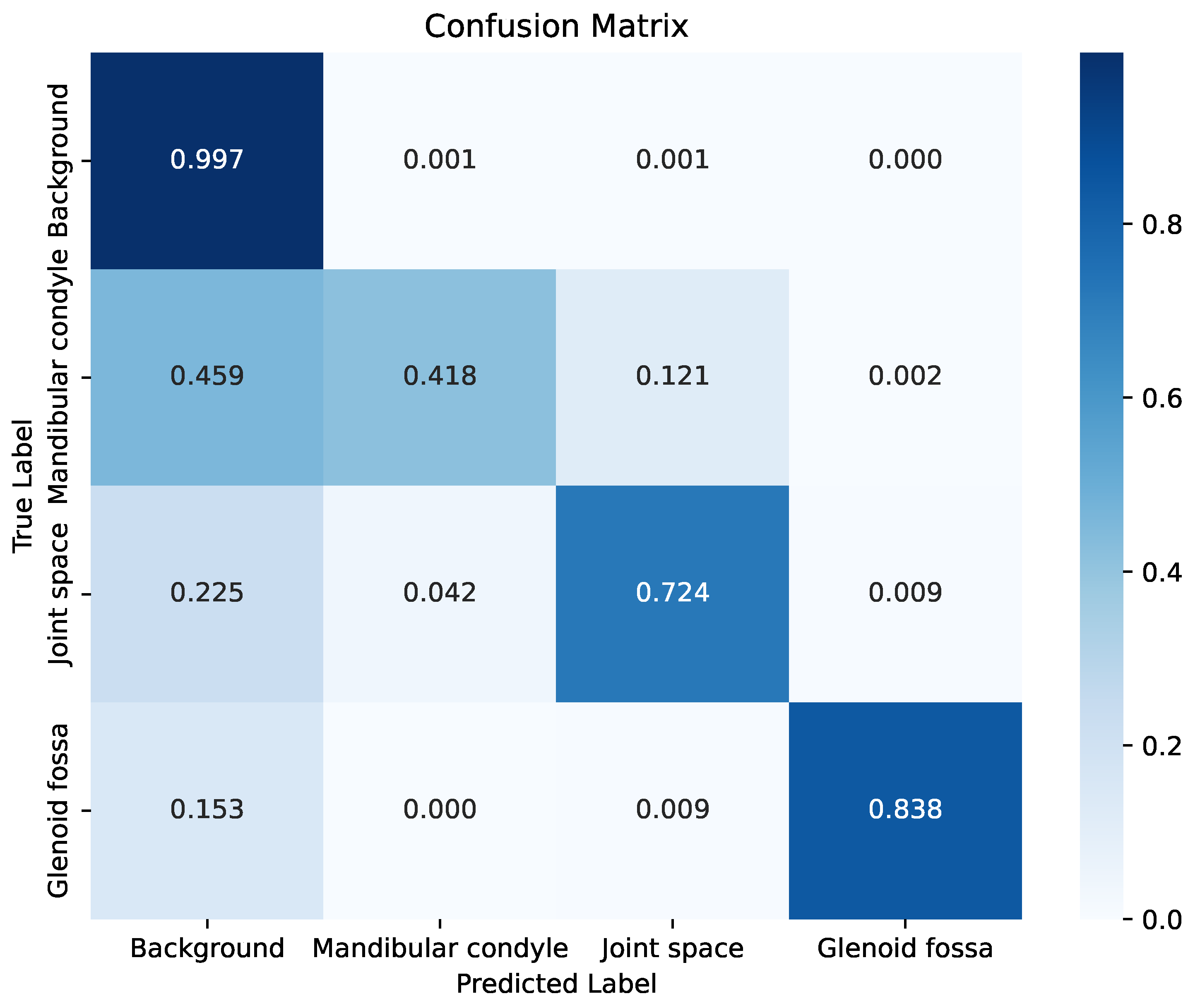
After evaluating the asymmetric kernel using the ILS algorithm, the best-performing architecture was employed for the final training phase. In order to maintain methodological consistency with the reference study used for comparison, we report a single training-testing split without cross-validation. This approach, as well as the small number of samples available for testing, undermines general conclusions from results. Nonetheless, notice tests evaluate performance in a pixel-wise basis, providing an in-depht view of segmentation behavior. To analyze the behavior of the proposed architecture concerning each class, the confusion matrix shown in Figure 7 was generated. This matrix was normalized in the range of 0 to 1, since the comparison between the segmented images and the ground-truth was performed at the pixel level. In this matrix, values close to 1 (represented in dark blue) indicate a high degree of similarity with the ground-truth, whereas values close to 0 (light tones) reflect low similarity between the predicted segmentation and the reference.
The confusion matrix provides insights into both correct classifications and the types of errors made by the model. As a large proportion of image pixels correspond to the background, the model achieved high accuracy in this class. However, the mandibular condyle resulted the most challenging structure to segment, yielding the lowest performance. This indicates that the model struggled to learn distinctive features for this region, leading to frequent misclassification of its pixels as background and, to a lesser extent, as joint space. In contrast, the joint space class exhibited notably better segmentation results, although some of its pixels were still incorrectly assigned to the background. A similar behavior was observed for the glenoid fossa, where residual confusion with background pixels persisted. The per-class Dice coefficients further clarify these findings, complementing the confusion matrix. The proposed model achieved Dice scores of 0.49 for the mandibular condyle, 0.80 for the joint space, and 0.86 for the glenoid fossa. These discrepancies can be partly attributed to the high entropy and speckle noise inherent to ultrasound images, which complicate the distinction between anatomical boundaries and non-informative regions.
In Figure 8, the behavior of the TP, TN, FP, and FN values can be observed for one of the three examples previously shown in Figure 2. The image shows the overlap between the prediction (highlighted in red) and the ground truth (highlighted in green). The yellow color represents the true positives (TP), i.e., the regions where the prediction matches the ground truth. The black color corresponds to the true negatives (TN), which belong to the background of the image. Meanwhile, red indicates the false positives (FP) areas that the model predicted as positive but are not whereas green represents the false negatives (FN), regions that the model failed to detect correctly. In Figure 8, the proposed model demonstrates strong performance in segmenting the three classes. However, some regions exhibit over-segmentation, which can be attributed to speckle noise and the inherent intensity variability of ultrasound images. These conditions may induce spurious activations, particularly when asymmetric kernels and channel recalibration mechanisms are employed. Nevertheless, the integration of SE blocks and asymmetric convolutions significantly enhances the sensitivity of the model to low-contrast structures.
A comparison was conducted between the proposed DenseUNet architecture and several representative state-of-the-art models, as shown in Table 1. The evaluated architectures include: Attention U-Net, U-Net++, DeepLabv3, SegResNet, SegResNet-VAE, Residual U-Net, and V-Net. In addition, the table presents a progressive evaluation of different architectural configurations, which can be interpreted as an ablation study demostrating the individual and combined impact of dense connections, SE blocks, and asymmetric kernels in the proposed DenseUNet variant. Four metrics were used for this comparison: Dice coefficient, precision, recall, and F1-score. As shown in Table 1, the proposed architecture achieved the best performance in terms of the Dice coefficient, reaching a value of 0.78. It was follows: closely by the Residual U-Net architecture proposed by Lasek et al. [4]. A similar trend was observed for the precision metric, where the proposed model also ranked first, with a value of 0.84. In terms of recall, the proposed architecture did not achieve the highest score, being outperformed by V-Net. However, this higher recall came at the cost of lower precision, indicating that V-Net exhibits a bias toward sensitivity, favoring the detection of true positives while also increasing the number of false positives.
Both the original DenseUNet and the DenseUNet-SE variants showed considerably lower performance, with the latter scoring below 0.30 across all evaluation metrics. The DenseUNet version with SE blocks performed worse than the baseline, likely because the SE mechanism focuses on global feature recalibration, which may not adequately capture specific structural patterns, such as elongated anatomical features. By relying on aggregated information from previous layers, SE blocks can overlook critical details related to the spatial orientation of these structures. In contrast, combining SE blocks with asymmetric kernels enables the network to more effectively focus on elongated features, which likely explains the substantial performance gains observed in the DenseUNet-SE model with asymmetric kernels. Meanwhile, other architectures such as Residual U-Net and SegResNet achieved balanced results across the evaluation metrics but were still outperformed by the proposed approach. These results further support the idea that the use of asymmetric kernels enhances the model’s ability to handle complex image segmentation tasks.
Overall, the results indicate a clear improvement from the original DenseUNet (Dice coefficient: 0.53) to the enhanced version incorporating asymmetric kernels (Dice: 0.78), highlighting the effectiveness of this structural modification. This gain can be attributed to the enhanced capacity of the asymmetric kernels to capture diverse spatial patterns. Furthermore, the proposed architecture achieved an average processing time of 0.16 s per image, demonstrating both high computational efficiency and robust segmentation performance.
The results of the proposed DenseUNet model outperformed those reported. The optimal model from [4], a Residual U-Net, primarily addresses the vanishing gradient issue. This aspect motivated the selection of the DenseUNet architecture, which utilizes dense connections to maintain gradient flow and better capture morphological features. Additionally, DenseNet and DenseUNet were developed as alternatives to ResNet and Residual U-Net architectures; it was considered relevant to compare them with the dataset from Lasek et al. [17].
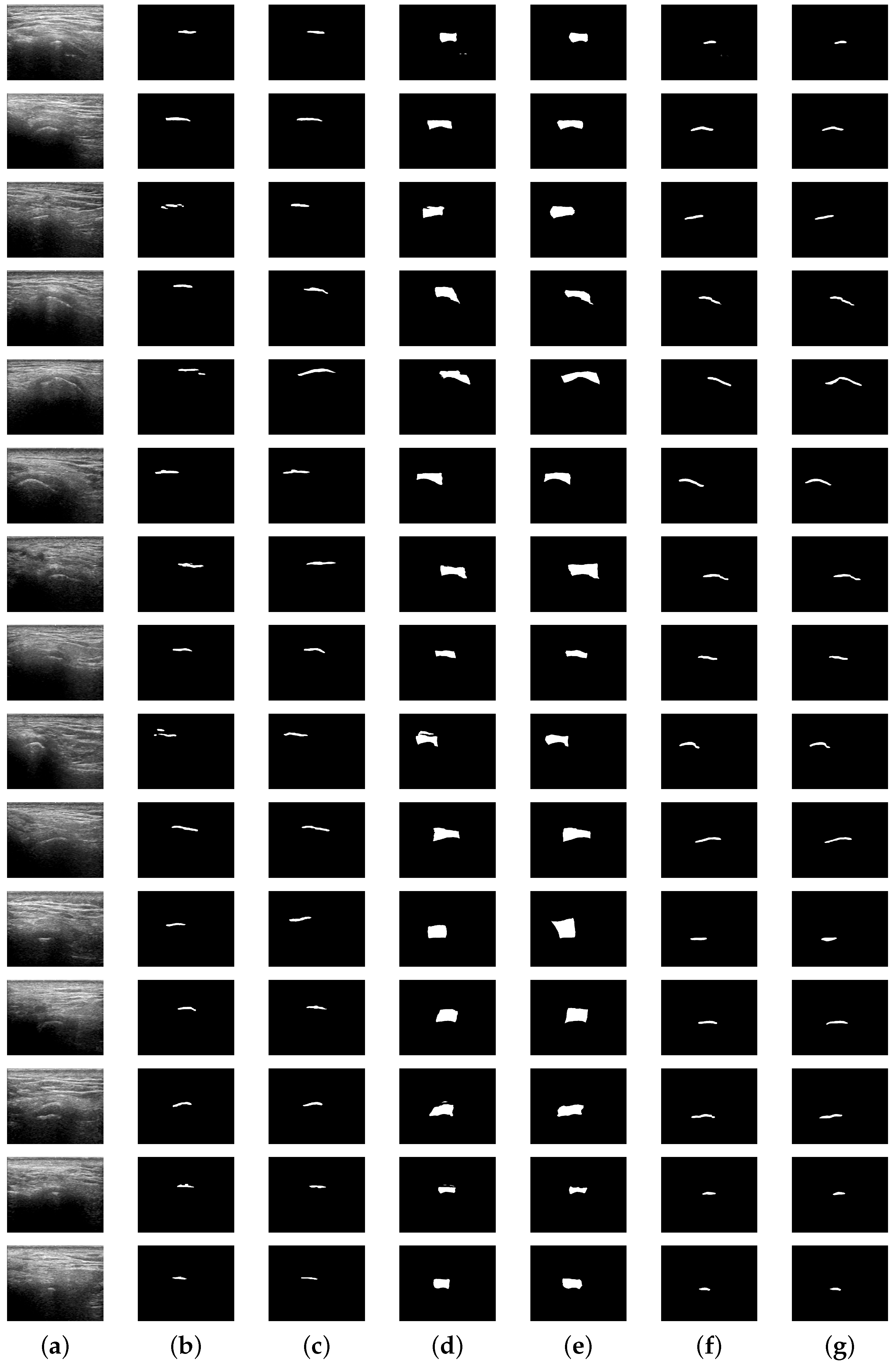
Figure 9 presents randomly selected examples of the segmentation performed by the proposed DenseUNet model, compared with the reference for each class. The results indicate that the segmentation generated by the model closely resemble the reference. However, as evidenced by the quantitative results, notable discrepancies persist, particularly in the mandibular condyle illustrated in Figure 9b, where the segmented structure is often incomplete or exhibits significant deviations from the reference. A similar, albeit less pronounced, issue is observed in the joint space and glenoid fossa, illustrated in Figure 9d,f.
Both the original images and the ground-truth exhibit a predominance of elongated shapes in the dataset images. Morphological characteristics motivated the application of asymmetric kernels, inspired by previous studies that have demonstrated their effectiveness in reducing computational costs [33,34]. However, we specifically evaluated their impact on TMJ structure segmentation. To assess their effectiveness, the performance of asymmetric filters (e.g., 1 × N) was compared with conventional kernels (e.g., 3 × 3, 5 × 5, 7 × 7, etc.) using the ILS algorithm. The results shown in Figure 6a indicate that asymmetric kernels outperformed conventional ones in this context. The key advantage of asymmetric kernels lies in their directional design, while conventional kernels are isotropic, capturing patterns equally in all directions, asymmetric filters prioritize specific orientations. Properties allow for better adaptation to elongated morphologies. In contrast, conventional kernels may under-represent or even omit critical structural information due to their omnidirectional nature. Lasek et al. [4] highlight the use of morphological operations as a post-processing step to refine segmentation outputs. In contrast, the proposed architecture does not incorporate any post-processing techniques, which suggests that the inclusion of such operations could further improve segmentation accuracy, particularly for structures with complex morphology, such as those in the Mandibular condyle.
5. Conclusions

The proposed architecture outperformed nine state-of-the-art models, achieving a Dice coefficient of 0.78, highlighting its superior segmentation capabilities on TMJ imagery (mandibular condyle, joint space and glenoid fossa). It also demonstrated efficient processing with an average inference time of 0.16 s per image. The use of the iterated local search algorithm to identify the optimal kernel combination underscores the value of employing optimization strategies in architectural design. Notably, the proposed model exhibited improved performance in segmenting the mandibular condyle, the most challenging and clinically critical class. This advantage can be attributed to the use of asymmetric filters. Unlike conventional isotropic kernels, which capture patterns equally in all directions and may under-represent elongated morphologies, asymmetric filters prioritize specific orientations, allowing for a more accurate representation of complex anatomical structures. Several avenues remain open for future research. These include evaluating the influence of image entropy, implementing techniques to optimize the learning dynamics of the architecture, and adapting the proposed modifications to other neural network architectures. By addressing these aspects, future architectures may achieve even higher levels of performance and robustness in complex medical image segmentation tasks.

Author Contributions

Conceptualization, E.F.D.-V. and I.C.-A.; Methodology, E.F.D.-V.; Software, E.F.D.-V.; Validation, E.F.D.-V.; Formal analysis, E.F.D.-V.; Investigation, E.F.D.-V.; Resources, I.C.-A.; Data curation, E.F.D.-V.; Writing—original draft, E.F.D.-V.; Writing—review & editing, I.C.-A., R.E.S.-Y. and J.C.-N.; Visualization, E.F.D.-V.; Supervision, R.E.S.-Y. and J.C.-N.; Project administration, I.C.-A. and J.C.-N.; Funding acquisition, R.E.S.-Y. All authors have read and agreed to the published version of the manuscript.

Funding

This research was funded by the Mexican Secretariat of Science, Humanities, Technology, and Innovation (SECIHTI) with scholarship grant No. 1081409 and the support under project IxM-SECIHTI No. 3097-7185.

Data Availability Statement

Restrictions apply to the availability of these data. Data were obtained from third party and are available at https://doi.org/10.5281/zenodo.14760859 with the permission of Lasek, J. et al. [17].

Acknowledgments

Edgar F. Duque-Vazquez gratefully acknowledges the Mexican Secretariat of Science, Humanities, Technology, and Innovation (SECIHTI) for the scholarship grant No. 1081409 and the support under project IxM-SECIHTI No. 3097-7185.

Conflicts of Interest

The authors declare no conflicts of interest.

References

  1. Wilkie, G.; Al-Ani, Z. Temporomandibular joint anatomy, function and clinical relevance. Br. Dent. J. 2022, 233, 539–546. [Google Scholar] [CrossRef]
  2. Gharavi, S.M.; Qiao, Y.; Faghihimehr, A.; Vossen, J. Imaging of the temporomandibular joint. Diagnostics 2022, 12, 1006. [Google Scholar] [CrossRef]
  3. Valesan, L.F.; Da-Cas, C.D.; Réus, J.C.; Denardin, A.C.S.; Garanhani, R.R.; Bonotto, D.; Januzzi, E.; de Souza, B.D.M. Prevalence of temporomandibular joint disorders: A systematic review and meta-analysis. Clin. Oral Investig. 2021, 25, 441–453. [Google Scholar] [CrossRef]
  4. Lasek, J.; Nurzynska, K.; Piórkowski, A.; Strzelecki, M.; Obuchowicz, R. Deep learning for ultrasonographic assessment of temporomandibular joint morphology. Tomography 2025, 11, 27. [Google Scholar] [CrossRef]
  5. Macedo De Sousa, B.; López-Valverde, N.; López-Valverde, A.; Caramelo, F.; Flores Fraile, J.; Herrero Payo, J.; Rodrigues, M.J. Different treatments in patients with temporomandibular joint disorders: A comparative randomized study. Medicina 2020, 56, 113. [Google Scholar] [CrossRef] [PubMed]
  6. Stocum, D.L.; Roberts, W.E. Part I: Development and physiology of the temporomandibular joint. Curr. Osteoporos. Rep. 2018, 16, 360–368. [Google Scholar] [CrossRef]
  7. Kazimierczak, W.; Kędziora, K.; Janiszewska-Olszowska, J.; Kazimierczak, N.; Serafin, Z. Noise-optimized CBCT imaging of temporomandibular joints-The impact of AI on image quality. J. Clin. Med. 2024, 13, 1502. [Google Scholar] [CrossRef] [PubMed]
  8. Wang, J.; Wang, S.; Zhang, Y. Deep learning on medical image analysis. CAAI Trans. Intell. Technol. 2025, 10, 1–35. [Google Scholar] [CrossRef]
  9. Manek, M.; Maita, I.; Bezerra Silva, D.F.; Pita de Melo, D.; Major, P.W.; Jaremko, J.L.; Almeida, F.T. Temporomandibular joint assessment in MRI images using artificial intelligence tools: Where are we now? A systematic review. Dentomaxillofacial Radiol. 2025, 54, 1–11. [Google Scholar] [CrossRef] [PubMed]
  10. Ito, S.; Mine, Y.; Yoshimi, Y.; Takeda, S.; Tanaka, A.; Onishi, A.; Peng, T.Y.; Nakamoto, T.; Nagasaki, T.; Kakimoto, N.; et al. Automated segmentation of articular disc of the temporomandibular joint on magnetic resonance images using deep learning. Sci. Rep. 2022, 12, 221. [Google Scholar] [CrossRef]
  11. Kim, J.Y.; Kim, D.; Jeon, K.J.; Kim, H.; Huh, J.K. Using deep learning to predict temporomandibular joint disc perforation based on magnetic resonance imaging. Sci. Rep. 2021, 11, 6680. [Google Scholar] [CrossRef]
  12. Li, M.; Punithakumar, K.; Major, P.W.; Le, L.H.; Nguyen, K.C.T.; Pacheco-Pereira, C.; Kaipatur, N.R.; Nebbe, B.; Jaremko, J.L.; Almeida, F.T. Temporomandibular joint segmentation in MRI images using deep learning. J. Dent. 2022, 127, 104345. [Google Scholar] [CrossRef]
  13. Mao, W.Y.; Fang, Y.Y.; Wang, Z.Z.; Liu, M.Q.; Sun, Y.; Wu, H.X.; Lei, J.; Fu, K.Y. Automated diagnosis and classification of temporomandibular joint degenerative joint disease via artificial intelligence using CBCT imaging. J. Dent. 2025, 154, 105592. [Google Scholar] [CrossRef] [PubMed]
  14. Choi, E.; Shin, S.; Lee, K.; An, T.; Lee, R.K.; Kim, S.; Son, Y.; Kim, S.T. Artificial intelligence-enhanced diagnosis of degenerative joint disease using temporomandibular joint panoramic radiography and joint noise data. Sci. Rep. 2025, 15, 1823. [Google Scholar] [CrossRef]
  15. Rehman, K.U.; Jianqiang, L.; Yasin, A.; Bilal, A.; Basheer, S.; Ullah, I.; Jabbar, M.K.; Tian, Y. A feature fusion attention-based deep learning algorithm for mammographic architectural distortion classification. IEEE J. Biomed. Health Inform. 2025, 1–12. [Google Scholar] [CrossRef]
  16. Pan, Y.; Zhang, Z.; Zhang, X.; Zeng, Z.; Tian, Y. YOLO-TARC: YOLOv10 with token attention and residual convolution for small void detection in root canal x-ray images. Sensors 2025, 25, 3036. [Google Scholar] [CrossRef]
  17. Lasek, J.; Nurzynska, K.; Piórkowski, A.; Strzelecki, M.; Obuchowicz, R. Ultrasound images of the temporomandibular joint with segmentations. Zenodo 2025. [Google Scholar] [CrossRef]
  18. Huang, G.; Liu, Z.; Van Der Maaten, L.; Weinberger, K.Q. Densely connected convolutional networks. In Proceedings of the IEEE Conference on Computer Vision and Pattern Recognition, Honolulu, HI, USA, 21–26 July 2017; pp. 4700–4708. [Google Scholar]
  19. Ronneberger, O.; Fischer, P.; Brox, T. U-Net: Convolutional Networks for Biomedical Image Segmentation. In Proceedings of the Medical Image Computing and Computer-Assisted Intervention (MICCAI 2015), Munich, Germany, 5–9 October 2015; Navab, N., Hornegger, J., Wells, W.M., Frangi, A.F., Eds.; Springer: Cham, Switzerland, 2015; pp. 234–241. [Google Scholar]
  20. Cao, Y.; Liu, S.; Peng, Y.; Li, J. DenseUNet: Densely connected UNet for electron microscopy image segmentation. IET Image Process. 2020, 14, 2682–2689. [Google Scholar] [CrossRef]
  21. Krithika Alias AnbuDevi, M.; Suganthi, K. Review of semantic segmentation of medical images using modified architectures of UNET. Diagnostics 2022, 12, 3064. [Google Scholar] [CrossRef] [PubMed]
  22. Lourenço, H.R.; Martin, O.C.; Stützle, T. Iterated Local Search. In Handbook of Metaheuristics; Glover, F., Kochenberger, G.A., Eds.; Springer: Boston, MA, USA, 2003; pp. 320–353. [Google Scholar] [CrossRef]
  23. Hoos, H.H.; Stützle, T. Stochastic Local Search algorithms: An overview. In Springer Handbook of Computational Intelligence; Kacprzyk, J., Pedrycz, W., Eds.; Springer: Berlin/Heidelberg, Germany, 2015; pp. 1085–1105. [Google Scholar] [CrossRef]
  24. Lourenço, H.R.; Martin, O.C.; Stützle, T. Iterated local search: Framework and applications. In Handbook of Metaheuristics; Springer: Berlin/Heidelberg, Germany, 2018; pp. 129–168. [Google Scholar]
  25. Subramanian, A.; Lourenço, H.R. Iterated Local Search. In Encyclopedia of Optimization; Pardalos, P.M., Prokopyev, O.A., Eds.; Springer International Publishing: Cham, Switzerland, 2020; pp. 1–10. [Google Scholar] [CrossRef]
  26. Hu, J.; Shen, L.; Sun, G. Squeeze-and-excitation networks. In Proceedings of the IEEE Conference on Computer Vision and Pattern Recognition, Salt Lake City, UT, USA, 18–22 June 2018; pp. 7132–7141. [Google Scholar]
  27. Oktay, O.; Schlemper, J.; Folgoc, L.L.; Lee, M.; Heinrich, M.; Misawa, K.; Mori, K.; McDonagh, S.; Hammerla, N.Y.; Kainz, B.; et al. Attention U-Net: Learning where to look for the pancreas. arXiv 2018, arXiv:1804.03999. [Google Scholar] [CrossRef]
  28. Zhou, Z.; Rahman Siddiquee, M.M.; Tajbakhsh, N.; Liang, J. UNet++: A nested U-Net architecture for medical image segmentation. In Deep Learning in Medical Image Analysis and Multimodal Learning for Clinical Decision Support: 4th International Workshop, DLMIA 2018, and 8th International Workshop, ML-CDS 2018, Held in Conjunction with MICCAI 2018, Granada, Spain, September 20, 2018, Proceedings 4; Springer: Berlin/Heidelberg, Germany, 2018; pp. 3–11. [Google Scholar]
  29. Chen, L.C.; Papandreou, G.; Schroff, F.; Adam, H. Rethinking atrous convolution for semantic image segmentation. arXiv 2017, arXiv:1706.05587. [Google Scholar] [CrossRef]
  30. Myronenko, A. 3D MRI brain tumor segmentation using autoencoder regularization. In Proceedings of the International MICCAI Brainlesion Workshop, Granada, Spain, 16 September 2018; Springer: Berlin/Heidelberg, Germany, 2018; pp. 311–320. [Google Scholar]
  31. Kerfoot, E.; Clough, J.; Oksuz, I.; Lee, J.; King, A.P.; Schnabel, J.A. Left-ventricle quantification using residual U-Net. In Statistical Atlases and Computational Models of the Heart. Atrial Segmentation and LV Quantification Challenges: 9th International Workshop, STACOM 2018, Held in Conjunction with MICCAI 2018, Granada, Spain, September 16, 2018, Revised Selected Papers 9; Springer: Berlin/Heidelberg, Germany, 2019; pp. 371–380. [Google Scholar]
  32. Milletari, F.; Navab, N.; Ahmadi, S.A. V-Net: Fully convolutional neural networks for volumetric medical image segmentation. In Proceedings of the 2016 Fourth International Conference on 3D Vision (3DV), Stanford, CA, USA, 25–28 October 2016; IEEE: Piscataway, NJ, USA, 2016; pp. 565–571. [Google Scholar]
  33. Ding, X.; Guo, Y.; Ding, G.; Han, J. Acnet: Strengthening the kernel skeletons for powerful CNN via asymmetric convolution blocks. In Proceedings of the IEEE/CVF International Conference on Computer Vision, Seoul, Republic of Korea, 27 October–2 November 2019; pp. 1911–1920. [Google Scholar]
  34. Szegedy, C.; Vanhoucke, V.; Ioffe, S.; Shlens, J.; Wojna, Z. Rethinking the inception architecture for computer vision. In Proceedings of the IEEE Conference on Computer Vision and Pattern Recognition, Las Vegas, NV, USA, 27–30 June 2016; pp. 2818–2826. [Google Scholar]
Figure 1. Schematic illustration of the temporomandibular joint highlighting the mandibular condyle, joint space, and temporal bone (adapted from [6]).
Symmetry 17 02014 g001
Figure 2. Examples of images from the dataset of Lasek et al. [17]: (a) Original grayscale image, (b) Mandibular condyle (Class 1), (c) Joint space (Class 2), and (d) Glenoid fossa of the temporal bone (Class 3).
Symmetry 17 02014 g002
Figure 3. Architecture of DenseUNet proposed by Cao et al. [20].
Symmetry 17 02014 g003
Figure 4. Dense block with the proposed modifications highlighted in red.
Symmetry 17 02014 g004
Figure 5. Proposed architecture based on the DenseUNet model from Cao et al. [20]. Black arrows denote the sequential data flow between blocks, with each output of the module being directly propagated to the next.
Symmetry 17 02014 g005
Figure 6. Comparison of Dice coefficient evolution and computation time for the kernel combinations explored using the ILS algorithm: (a) Dice coefficient (Evolution of the Dice coefficient for the kernel combinations explored using the ILS algorithm. The asymmetric kernel of size 1 × 13 obtained the highest Dice coefficient value.), (b) Computation time (Computation time evolution of each DenseUNet model based on the kernel combinations explored using the ILS algorithm, evaluated on the training set with ground-truth annotations.).
Symmetry 17 02014 g006
Figure 7. Normalized confusion matrix of the proposed architecture. Values are scaled to the [0, 1] range to better illustrate the classification performance for each class.
Symmetry 17 02014 g007
Figure 8. Visual comparison between the segmentation producen by the proposed model and the ground-truth, showing FP, FN, TP, and TN, for a worst-case example.
Symmetry 17 02014 g008
Figure 9. Subset of segmentation results obtained by the proposed architecture alongside their corresponding ground-truth. (a) Original image, (b) Segmentation for Mandibular condyle, (c) Ground-truth for Mandibular condyle, (d) Segmentation for Joint space, (e) Ground-truth for Joint space, (f) Segmentation for Glenoid fossa, (g) Ground-truth for Glenoid fossa.
Symmetry 17 02014 g009
Table 1. A comparison of the results obtained by the proposed DenseUNet architecture against the reference models.
ModelDicePrecisionRecallF1-Score
Attention U-Net [27]0.640.670.650.66
U-Net ++ [28]0.720.740.720.73
DeepLabv3 [29]0.720.750.720.73
SegResNet [30]0.730.730.740.73
SegResNet-VAE [30]0.730.730.740.73
Residual U-Net [31]0.750.770.750.76
V-Net [32]0.660.600.790.68
DenseUNet [20]0.530.760.460.57
DenseUNet-SE0.240.230.250.24
Proposed0.780.840.740.79
Bold value indicates the higher performance when comparing models and using a specific metric.
Disclaimer/Publisher’s Note: The statements, opinions and data contained in all publications are solely those of the individual author(s) and contributor(s) and not of MDPI and/or the editor(s). MDPI and/or the editor(s) disclaim responsibility for any injury to people or property resulting from any ideas, methods, instructions or products referred to in the content.