Article

Taylor-Type Direct-Discrete-Time Integral Recurrent Neural Network with Noise Tolerance for Discrete-Time-Varying Linear Matrix Problems with Symmetric Boundary Constraints

1
School of Artificial Intelligence, Guangzhou Maritime University, Guangzhou 510275, China
2
School of Cyber Security, Guangdong Polytechnic Normal University, Guangzhou 510635, China
3
School of Information Engineering, Jiangxi University of Science and Technology, Ganzhou 341000, China
*
Author to whom correspondence should be addressed.
Symmetry 2025, 17(11), 1975; https://doi.org/10.3390/sym17111975
Submission received: 23 October 2025 / Revised: 10 November 2025 / Accepted: 13 November 2025 / Published: 15 November 2025
(This article belongs to the Section Computer)

Abstract

Various types of noise interference often challenge the solution of discrete time-varying linear matrix problems with boundary constraints in practical engineering applications. To address this issue, this paper proposes a Taylor-type direct-discrete-time integral noise-immune recurrent neural network (TD-IRNN) model. Specifically, the model is constructed by transforming the bounded discrete linear matrix problem into a unified discrete matrix formulation and incorporating an error accumulation term during the design process. The proposed TD-IRNN model not only eliminates the need for continuous-environment conversion but also significantly enhances its noise immunity. Theoretical analysis demonstrates that the model exhibits excellent convergence and stability under different noise conditions. Numerical experiments and a robotic manipulator trajectory tracking experiment further validate the effectiveness and practical applicability of the TD-IRNN model in complex environments.

1. Introduction

The discrete time-varying linear matrix problems not only constitute an important research topic in mathematical analysis [1,2,3], but also demonstrate key theoretical value and practical significance in the intersection of engineering and science, such as control system design [4,5], robotic dynamics modeling [6], and intelligent learning algorithms [7]. Such problems involve solving dynamic system matrix equations at discrete time steps [8,9], generally formulated as finding a solution vector x k that satisfies A k x k = b k , where both the coefficient matrix A k and the right-hand vector b k vary over time. This time-dependent nature renders discrete time-varying linear problems more challenging than static linear problems while better aligning with the dynamic characteristics of real-world engineering systems [10]. In practical applications, solving such problems requires not only imposing boundary constraints on variables but also addressing inevitable noise interference. Boundary constraints originate from diverse sources, including physical system limitations [11,12] (such as the joint angle range of robot arms), practical engineering design requirements [13,14] (such as amplitude limitations of control signals), or feasible domain definitions for optimization problems [15]. Although these constraints and noise increase solution complexity, they also enhance the practical significance and applicability of solution methodologies.
Recurrent neural networks (RNNs) [16,17,18,19,20,21] are specifically designed for processing sequential data and dynamic systems due to their capability to capture temporal dependencies and dynamic evolution [22]. This inherent characteristic makes them particularly suitable for solving time-varying linear matrix problems [23]. For instance, Xu et al. [24] developed a continuous-time RNN (CTRNN) model for solving time-dependent linear equations with boundary constraints, successfully applying it to time-varying linear equations and inequality systems. However, CTRNN implementation faces significant hardware challenges [25]. To facilitate hardware realization, researchers often discretize CTRNN using numerical methods [26]. For example, Cang et al. [27] proposed a novel discrete-time RNN (DTRNN) model based on the Taylor difference formula for solving time-dependent linear equation problems with boundary constraints. Nevertheless, noise interference remains unavoidable in practical RNN implementations, making the enhancement of robustness a critical requirement for developing reliable RNN models for time-varying problems. Jin et al. [28] designed an integral enhanced RNN model by incorporating integral techniques to achieve inherent noise immunity for continuous time-varying problems. On the basis of continuous-time domain research, Zheng et al. [29] proposed a discrete error redefinition neural network model to solve the time-varying quadratic programming problem. Notably, all the aforementioned discrete models are established based on the continuous-time domain RNNs [30].
In summary, the above studies all follow a representative technical route: first establishing a theoretical model in the continuous-time domain, then transforming it into a discrete-time model through numerical discretization. This approach maintains theoretical consistency with the framework of solving discrete time-varying problems based on continuous-time environments. However, Shi et al. proposed a new technique called the Taylor direct-discrete RNN (TDRNN) model [31], filling the previous research gap of relying on continuous-time environments through direct discretization techniques. Nonetheless, research on constrained and noisy environments within the direct discretization framework remains limited. To bridge this research gap, we introduce an error accumulation term and propose a Taylor-type direct-discrete-time integral noise-immune RNN (TD-IRNN) model to solve discrete time-varying linear matrix problems with boundary constraints. Compared with models derived from the discretization of continuous-time models [26,27], the TD-IRNN adopts a direct discretization approach, eliminating the need for continuous-to-discrete transformation and improving computational efficiency. Additionally, a key advantage of the TD-IRNN model lies in the embedded error integral term, which endows it with inherent noise tolerance, and this feature is absent in the TDRNN model [31]. The aforementioned differences between the proposed model and some existing discrete models are summarized in Table 1.
The TD-IRNN model proposed in this paper, leveraging its core advantages in handling discrete time-varying problems with boundary constraints and inherent noise tolerance, exhibits tremendous application potential in a broader range of intelligent system fields beyond the scope of this study. For instance, the core computational task of adaptive human-robot interaction torque estimation in lower limb rehabilitation robots can usually be transformed into a constrained time-varying estimation problem under sensor noise, which is highly consistent with the technical advantages of the TD-IRNN. Similarly, in the fields of batch process control and fault-tolerant consensus of multi-agent systems, online optimization or control law calculation often requires solving time-varying linear or linearized subproblems subject to operational constraints. The TD-IRNN model can serve as a powerful and robust computational engine within advanced frameworks such as event-triggered control. Its ability to process such problems in real time while satisfying constraints and suppressing noise fully demonstrates its versatility and potential impact in various adaptive and robust control fields.
The remainder of this article is organized as follows. Section 2 introduces the process of establishing the problem model and existing discrete models. Section 3 elaborates on the construction process of the proposed TD-IRNN model. Section 4 presents detailed theoretical analyses demonstrating the convergence and robustness of the TD-IRNN model. Section 5 conducts numerical experiments and a robot arm application experiment to further validate the effectiveness and applicability of the TD-IRNN model. Section 6 discusses the potential extension of the TD-IRNN model to nonlinear systems and complex constraint scenarios. Section 7 summarizes the entire article. The article framework is illustrated in Figure 1. The main contributions of this article are summarized as follows:
(1)
A novel TD-IRNN model is proposed for solving discrete time-varying linear matrix problem with boundary constraints without relying on continuous-time theory. The complete model formulation and detailed derivation process are provided.
(2)
The convergence and robustness properties of the TD-IRNN model are rigorously proven through theoretical derivations. Specifically, the enhanced model achieves exact convergence when solving discrete time-varying linear matrix problem with boundary constraints and maintains convergence under three distinct types of noise interference.
(3)
Comparative numerical experiments with three discrete models confirm the convergence performance of the TD-IRNN model in solving the target problem. Meanwhile, the model demonstrates consistent convergence while satisfying boundary constraints under constant, linear, and bounded random noise conditions. Furthermore, two robotic arm trajectory tracking experiments validate the practicality and effectiveness of the TD-IRNN model in practical applications.

2. Problem Formulation and Existing Discrete Model

This section first presents the formulation of the discrete time-varying linear matrix problem with boundary constraints and then provides three existing discrete models for comparison. For convenience, the variables commonly used in this paper are presented below.
Q k Time-varying augmented matrix
w k Time-varying augmented matrix
r k Time-varying vector
x + The upper bound of the variable x k
x The lower bound of the variable x k
P k Time-varying augmented matrix
P k + the pseudoinverse of matrix P k
τ Sampling gap
ω Design parameter
λ Integral parameter of the TD-IRNN model
E k Error function E k = Q k w k r k
Y k j Error state vector
e k j The jth element of E k
O ( ) Truncation error vector

2.1. Problem Formulation

The discrete time-varying linear matrix problem with symmetric boundary constraints [32] is formulated as follows:
A k x k = b k x x k x +
where A k R m × n denotes a time-varying full rank matrix, and b k R m represents a time-varying vector. The unknown vector x k R n is to be determined, subject to the symmetric boundary constraints defined by x ± . The objective of this study is to compute x k using feasible numerical methods while ensuring that the solution remains within the prescribed bounds.
The constraint conditions in (1) can be rewritten as:
C x k ϑ ,
where C = [ I ; I ] R 2 n × n and ϑ = [ x ; x + ] R 2 n . Then, (1) can be transformed into solving the following system by introducing a nonnegative term:
A k x k b k = 0 C x k ϑ + D k y k = 0
where D k = d i a g y k 1 , , y k 2 n R 2 n × 2 n is a diagonal matrix, I R n × n is an identity matrix, and y k is an unknown vector that must still be determined when solving it. The above equation can be expressed as a matrix vector equation as follows:
Q k w k r k = 0 .
Among them, the augmented matrix Q k R ( m + 2 n ) × 3 n , vectors w k R 3 n , and r k R m + 2 n are represented by Q k = A k 0 C D k , w k = x k y k , and r k = b k ϑ .
It is worth noting that the problem to be solved in this paper is the constrained discrete time-varying linear matrix problem shown in (1), but directly solving this constrained problem poses certain difficulties. Therefore, the original problem can be equivalently transformed into the unified form of (2) through the aforementioned transformation method, thereby facilitating subsequent solution. The primary advantage of ZNN-based schemes lies in their ability to solve time-varying problems in real time through dynamic evolution equations. Unlike conventional numerical methods designed for static problems, ZNN can effectively track the time-varying solution x k . For scenarios involving asymmetric inequality constraints, these asymmetric boundary constraints in (1) are transformed into the unified formulation of (2), thereby directly incorporating such constraints into the dynamic system to be solved. The proposed TD-IRNN model builds upon this powerful ZNN framework, thus inheriting its strengths in handling dynamic systems with boundary constraints.

2.2. EDTZNN Model

Firstly, the continuous-time zeroing neural network model for solving the discrete time-varying linear matrix problem with boundary constraints (1) is given by
w ˙ ( t ) = P ( t ) + ω Q ( t ) w ( t ) r ( t ) + M ( t ) w ( t ) r ˙ ( t ) ,
where ω > 0 denotes the design parameter, w ˙ ( t ) and r ˙ ( t ) denote the time derivatives of w ( t ) and r ( t ) , respectively. The augmented matrices P ( t ) R ( m + 2 n ) × 3 n and M ( t ) R ( m + 2 n ) × 3 n can be expressed as
P ( t ) = A ( t ) 0 C 2 D ( t ) and M ( t ) = A ˙ ( t ) 0 0 0 .
Then, the Euler discretization method w ˙ k = ( w k + 1 w k ) / τ  [27] is employed to discretize (3), and the resulting Euler discrete-time zeroing neural network (EDTZNN) model [27] is formulated as follows:
w k + 1 = w k s P k + ( Q k w k r k ) τ P k + ( M k w k r ˙ k ) ,
where s = ω τ and τ = t k + 1 t k represents sampling gap.

2.3. TDTZNN Model

In addition to the Euler discretization method mentioned above, Taylor discretization is also a commonly used discretization technique. A Taylor discretization formula with higher precision, as referenced in [26], is formulated as follows:
w ˙ k = 2 w k + 1 3 w k + 2 w k 1 w k 2 2 τ .
By substituting (3) into (5), the Taylor discrete-time zeroing neural network (TDTZNN) model can be derived as follows:
w k + 1 = 3 2 x k x k 1 + 1 2 x k 2 τ P k + ( M k w k r ˙ k ) τ P k + ω Q k w k r k .

2.4. TDRNN Model

Based on the idea of direct discretization, the direct discrete recurrent neural network (TDRNN) model proposed by Shi et al. [31] for solving the discrete time-varying linear matrix problem with boundary constraints (1) is formulated as follows:
w k + 1 = ( ω 1 ) Q k 1 ( Q k w k r k ) τ Q k 1 ( Q ˙ k w k r ˙ k ) + w k ,
where ω denotes a design parameter.
Note that the TDRNN model (7) is constructed to solve problem (1) at discrete time steps and does not require a discrete transformation from a continuous model to a discrete model, which differs from the EDTZNN (4) and TDTZNN (6) models. The TD-IRNN model proposed in this paper is also constructed by the direct discretization approach.

3. Novel TD-IRNN Model

This section presents the construction of the TD-IRNN model. First, the error function at time k and k + 1 is defined based on (2) as follows:
E k = Q k w k r k
and
E k + 1 = Q k + 1 w k + 1 r k + 1 .
Inspired by the idea of direct discretization [33] and for the convenience of subsequent calculations, the partial derivatives of E k with respect to t k and w k are given as follows:
d E k / d t k = Q ˙ k w k r ˙ k ,
and
E k / w k = Q k .
To derive a discretized model, the second-order Taylor expansion [34] is introduced, yielding:
E k + 1 = E k + ( E k / w k ) ( w k + 1 w k ) + ( d E k / d t k ) ( t k + 1 t k ) + O ( τ 2 ) = E k + Q k ( w k + 1 w k ) + ( Q ˙ k w k r ˙ k ) τ + O ( τ 2 ) .
When k , let E k + 1 = ω E k λ i = 0 k E i , where 0 < ω < 1 , and 0 < λ < 2 + 2 ω denotes integral parameter. The error integral term i = 0 k E i incorporated into the design formula E k + 1 = ω E k λ i = 0 k E i directly embeds the inherent noise tolerance into the discrete-time dynamic characteristics, providing an intrinsic model-level mechanism for actively suppressing errors caused by noise and significantly enhancing the noise resistance performance of the TD-IRNN model. By ignoring truncation errors O ( τ 2 ) , we further obtain
E k + 1 E k = ( ω 1 ) E k λ i = 0 k E i = Q k ( w k + 1 w k ) + ( Q ˙ k w k r ˙ k ) τ ,
and then, (11) can be converted into
( ω 1 ) ( Q k w k r k ) λ i = 0 k E i = Q k ( w k + 1 w k ) + ( Q ˙ k w k r ˙ k ) τ .
The TD-IRNN model is obtained as follows:
w k + 1 = ( ω 1 ) Q k 1 ( Q k w k r k ) τ Q k 1 ( Q ˙ k w k r ˙ k ) λ Q k 1 i = 0 k E i + w k .
It should be noted that the performance of the TD-IRNN model is influenced by both parameters ω and λ , and the reasonable selection of these two parameters is crucial for the model to achieve optimal performance. The core function of parameter ω is to control the convergence speed of the model. The closer ω is to 0, the slower the initial convergence speed but the higher the final convergence accuracy. Conversely, the closer ω is to 1, the faster the initial convergence speed but the lower the final convergence accuracy. Therefore, the suitable selection range of ω is 0.5 to 0.8. In practical applications, the specific value of ω can be further determined according to the priority requirements for convergence speed and accuracy in specific scenarios. Parameter λ mainly affects the noise resistance of the model, and its value needs to be adjusted collaboratively with the selected value of ω . For most application scenarios, an efficient parameter selection strategy can be adopted: first set λ to 1, and then adjust its value according to the actually observed noise characteristics.

4. Theoretical Analyses

This section presents rigorous theoretical analyses of both convergence and stability properties [35] for the proposed TD-IRNN model (12).
Theorem 1.
Consider the TD-IRNN model (12) applied to solve the discrete time-varying linear matrix problem with boundary constraints (1). If the design parameters are chosen such that 0 < ω < 1 and 0 < λ < 2 + 2 ω then the model is 0-stable and its solution converges to the theoretical solution with a steady-state residual error of O ( τ 2 ) .
Proof. 
According to the design of the TD-IRNN Model (12) in Section 3, the design formula is
E k + 1 = ω E k λ i = 0 k E i + O ( τ 2 ) .
The design formula (13) introduces an additional error accumulation term, whose primary motivation is to systematically enhance the robustness of the TD-IRNN model (12) under noise interference. At time k, we can obtain:
E k = ω E k 1 λ i = 0 k E i + O ( τ 2 ) .
Subsequently, subtracting (14) from (13) yields:
E k + 1 = ( 1 λ + ω ) E k ω E k 1 + O ( τ 2 ) .
Thus, the characteristic polynomial can be expressed as
ρ 2 ( 1 λ + ω ) ρ + ω = 0 ,
where 0 < ω < 1 and 0 < λ < 2 + 2 ω . According to the Jury stability criterion, it is known that the roots of the characteristic polynomial (i.e., ρ 1 = ( 1 λ + ω ) + ( 1 λ + ω ) 2 4 ω 2 and ρ 2 = ( 1 λ + ω ) ( 1 λ + ω ) 2 4 ω 2 ) lie strictly inside the unit circle. Therefore, the TD-IRNN model (12) is 0-stable.
According to the second-order Taylor expansion formula (10), the following equation can be derived:
Q k ( w k + 1 w k ) = E k + 1 E k ( Q ˙ k w k r ˙ k ) τ O ( τ 2 ) .
Multiplying both sides by Q k 1 , we can rewrite (16) as
w k + 1 = w k + Q k 1 ( E k + 1 E k ( Q ˙ k w k r ˙ k ) τ ) Q k 1 O ( τ 2 ) .
Then, substituting (11) into (17), we can obtain:
w k + 1 = w k + Q k 1 ( ω 1 ) E k λ i = 0 k E i ( Q ˙ k w k r ˙ k ) τ Q k 1 O ( τ 2 )
with Q k 1 O ( τ 2 ) = O ( τ 2 ) , so the truncation error of the TD-IRNN model (12) for solving the discrete time-varying linear matrix problem with boundary constraints (1) is O ( τ 2 ) . The proof is completed in this way.    □
Theorem 2.
Under the conditions of Theorem 1, the TD-IRNN model (12) can generate a time-dependent solution of (1).
Proof. 
According to the analysis result of Theorem 1, the solution x k obtained by the TD-IRNN model (12) can converge to the theoretical solution x k of (1). Mathematically, x k x k when k is sufficiently large [36]. Therefore, from (2) and the definitions of Q k and r k , we can obtain:
lim k A k x k b k C x k ϑ = lim k 0 D k y k ,
where D k y k > 0 , the following result can be obtained:
lim k ( A k x k b k ) = 0 x lim k ( x k ) x + .
From this result, it can be concluded that the TD-IRNN model (12) is capable of generating the time-dependent solution to the discrete time-varying linear matrix problem with boundary constraints (1). The proof is completed in this way.    □
Theorem 3.
Under the conditions of Theorem 1, the steady-state computational error lim k E k 2 of the TD-IRNN model (12) is O ( τ 2 ) , where · 2 is the Euclidean norm of a vector.
Proof. 
Let e k j be the jth element of E k . Then, (15) can be rewritten as follows:
e k + 1 j = ( 1 λ + ω ) e k j ω e k 1 j + O ( τ 2 ) .
Defining a new error state Y k + 1 = [ e k + 1 j , e k j ] T , Equation (18) can be written in the following form:
Y k + 1 j = G Y k j + O ( τ 2 ) ,
where matrix G is defined as
G = 1 λ + ω ω 1 0 .
Therefore, from (19), we can obtain
| | Y k + 1 j | | 2 = | | G Y k j + O ( τ 2 ) | | 2 | | G | | 2 | | Y k j | | 2 + O ( τ 2 ) | | G | | 2 2 | | Y k 1 j | | 2 + O ( τ 2 ) | | G | | 2 k | | Y 1 j | | 2 + O ( τ 2 ) .
It can be easily concluded that the absolute value of the real part of G is less than 1, therefore lim k G 2 k = 0 , and
lim k Y k + 1 j 2 = O ( τ 2 ) .
Consequently, according to the definitions of Y k + 1 j and e k j , the steady-state calculation error lim k E k + 1 2 is O ( τ 2 ) . The proof is completed in this way.    □
Theorem 4.
Consider the TD-IRNN model (12) under constant noise pollution n ( t k ) = ν . If the conditions of Theorem 1 hold, the steady-state calculation error lim k E k 2 of the TD-IRNN model (12) is O ( τ 2 ) .
Proof. 
Considering the interference of constant noise, the design formula of TD-IRNN model (12) can be expressed as
E k + 1 = ω E k λ i = 0 k E i + ν + O ( τ 2 )
of which the jth subsystem can be formulated as
e k + 1 j = ω e k j λ i = 0 k e i + ν j + O ( τ 2 ) .
By applying the Z-transform to the above Equation (20), we can obtain
z e z j z e j ( 0 ) = ω e z j λ z z 1 e z j + ν j z z 1 + O ( τ 2 ) .
Based on the aforementioned Equation (21), the transfer function e z j can be derived as
e z j = z ( z 1 ) e j ( 0 ) + ν j z ( z ω ) ( z 1 ) + λ z + O ( τ 2 ) .
According to the terminal value theorem of Z-transform, we have:
lim k e k j = lim z 1 ( z 1 ) e z j = lim z 1 ( z 1 ) z ( z 1 ) e j ( 0 ) + ν j z ( z ω ) ( z 1 ) + λ z + O ( τ 2 ) = O ( τ 2 ) .
The proof is completed in this way.    □
Theorem 5.
Consider the TD-IRNN model (12) under bounded random noise pollution n ( t ) = σ . If the conditions of Theorem 1 hold, then the TD-IRNN model (12) has stability with bounded-input bounded-output (BIBO), and the corresponding steady-state calculation error is bounded by 2 n sup 1 i k , 1 j n | σ i j | / ( 1 G 2 ) + O ( τ 2 ) .
Proof. 
The TD-IRNN model (12) is a linear system that can be divided into two parts by separately considering the random noise σ and O ( τ 2 ) . Similar to the proof in Theorem 4, the jth subsystem of the TD-IRNN model (12) under the contamination of boundary random noise is:
e k + 1 j = ω e k j λ i = 0 k e i + σ k j + O ( τ 2 ) .
Similar to Theorem 3, subtracting the formula at time k from that at time k + 1 yields:
e k + 1 j = ( 1 λ + ω ) e k j ω e k 1 j + σ k j σ k 1 j .
Let η k j = σ k j σ k 1 j , 0 T , the above equation is rearranged into the following state space equation:
Y k + 1 j = G Y k j + η k j .
Then, we get
| | Y k + 1 j | | 2 | | G | | 2 | | Y k j | | 2 + | | η k j | | 2 | | G | | 2 2 | | G Y k 1 j | | 2 + | | G | | 2 | | η k 1 j | | 2 + | | η k j | | 2 | | G | | 2 k | | G Y 1 j | | 2 + | | G | | 2 k 1 | | η 1 j | | 2 + + | | η k j | | 2 < | | G | | 2 k | | G Y 1 j | | 2 + max 1 i k | | η k j | | 2 / ( 1 | | G | | 2 ) < | | G | | 2 k | | G Y 1 j | | 2 + 2 max 1 i k | σ k j | 2 / ( 1 | | G | | 2 ) .
In addition, we know lim k G 2 k = 0 , and further we can obtain
lim k Y k + 1 j 2 < 2 max 1 i k | σ k j | 2 / ( 1 G 2 ) .
Therefore, we can conclude that
lim k E k 2 < 2 n sup 1 i k , 1 j n | σ i j | / ( 1 G 2 ) + O ( τ 2 ) .
The proof is thus completed.    □
Due to the introduction of the error integral term λ i = 0 k E i in the paper, it is necessary to discuss the computational complexity and memory cost of the TD-IRNN model (12). The core computation of the TD-IRNN model (12) at each time step involves matrix-vector multiplication and one matrix inversion, with a computational complexity of O ( n 3 ) for the direct method. The introduced integral term adds an O ( n ) computational overhead per time step without altering the dominant O ( n 3 ) complexity. The introduction of the integral term incurs a memory cost of O ( n ) . While its standard implementation leads to linear memory growth over time, this can be efficiently bounded to O ( n ) using a forgetting mechanism like the exponential moving average. Therefore, the memory cost of the TD-IRNN model (12) remains controllable. The matrix inversion and matrix-vector multiplication, which are the most computationally intensive parts in the TD-IRNN model (12), are both standard linear algebra operations and can be efficiently parallelized on GPU architectures.

5. Simulation Experiment

This section verifies the convergence performance and robustness of the proposed TD-IRNN model (12) in solving the discrete time-varying constraint problem (1) in different noise environments through two complementary methods: numerical simulation and robot arm experiments. In the experiments, the augmented matrix Q K may exhibit ill-conditioning or be near-singular. Thus, all models utilize pseudoinverse Q K + .

5.1. Numerical Experiment

In this subsection, numerical simulations and comparative experiments will be conducted to verify the effectiveness and superiority of the proposed TD-IRNN model (12) in solving discrete time-varying linear matrix problem with boundary constraints (1). Among them, Algorithm 1 details the implementation procedure of the numerical experiments. In the comparative experiment section, the EDTZNN model (4), TDTZNN model (6), TDRNN model (7), and the proposed TD-IRNN model (12) are respectively adopted to solve the following discrete time-varying linear matrix problem with boundary constraints:
A ( t ) = 3 + cos ( 3 t ) , 1 + sin ( 6 t ) , 6 sin t cos t b ( t ) = sin t cos t x + = x = 0.4 , 0.4 , 0.4 .
Algorithm 1 Numerical Implementation of TD-IRNN Model (12)
Require: 
The discrete time-variant matrix A k R m × n , the discrete time-varying vectors b k R m and the upper and lower boundaries of unknown values x ± ; sampling period τ , design parameter ω and each computational time interval [ t k , t k + 1 ) [ t 0 , t f ] [ 0 , + ) ;
1:
Calculation: Transform a system of equations with symmetric boundary constraints (1) into a single linear equation problem (2);
2:
Initialize: w 0 , Q 0 , Q ˙ 0 , r 0 and r ˙ 0 ;
3:
Calculate: w 1 , Q ˙ 1 , R ˙ 1 and x 2 ;
4:
for  t 2 t f  do
5:
    Calculate: Q ˙ k and r ˙ k ;
6:
    Calculate: w k + 1 via the TD-IRNN model (12);
7:
    Output: Calculate the value x k + 1 and calculate the residual error E k + 1 F of the TD-IRNN model (12);
8:
end for
9:
Stop: Numerical implementation of TD-IRNN model (12) is completed.
The parameter set for the experiment is defined as follows: the convergence parameter ω = 0.7 , the design parameter λ = 1 , and the sampling gap τ = 0.001 . The influence of noise on the TD-IRNN model (12) is systematically investigated through three distinct noise scenarios: a constant noise vector with each element fixed at 20, a linear noise vector where each element follows 20 + t k , and a bounded random noise vector with elements uniformly distributed between 19 and 21. The selected noise level is significantly larger than the magnitude of the true solution vector x k . This setup aims to verify the robustness of the TD-IRNN model (12) under severe yet practically meaningful disturbances, providing strong evidence for the inherent noise tolerance of this model (12).
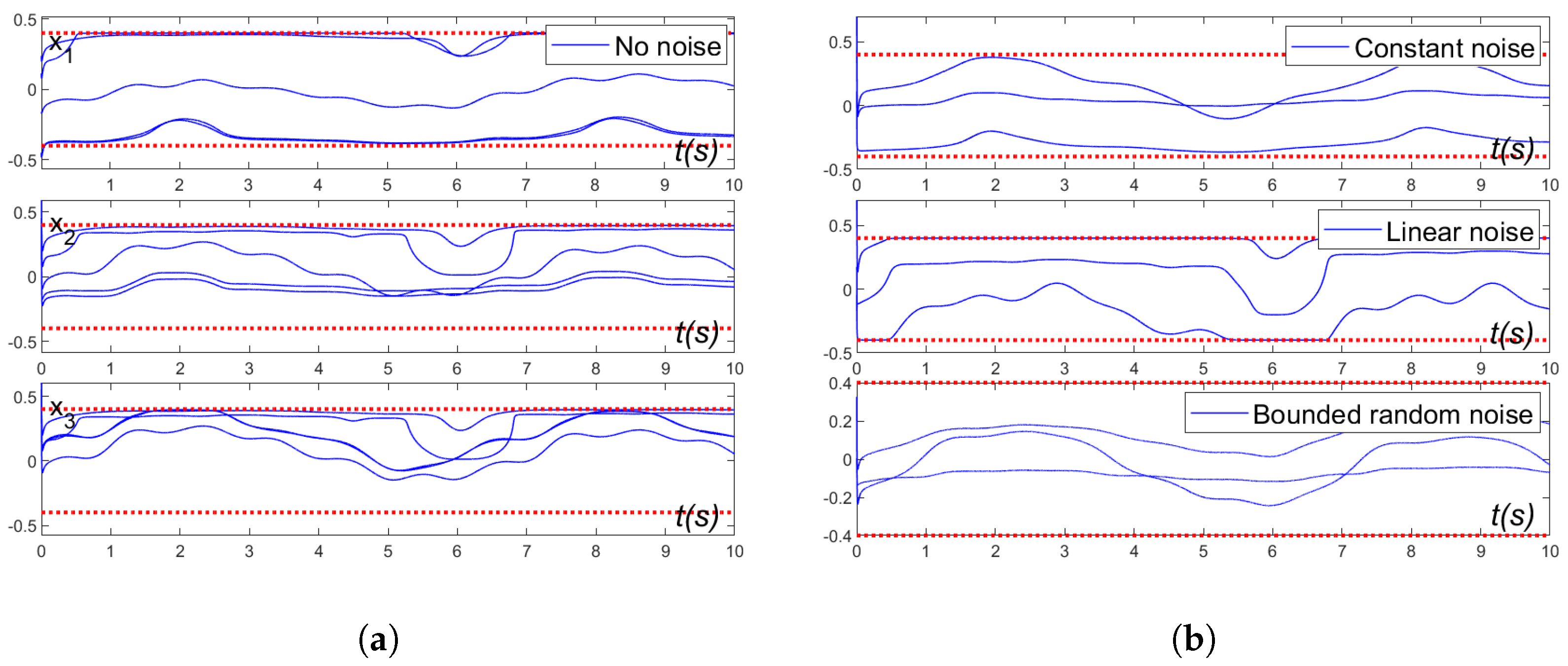
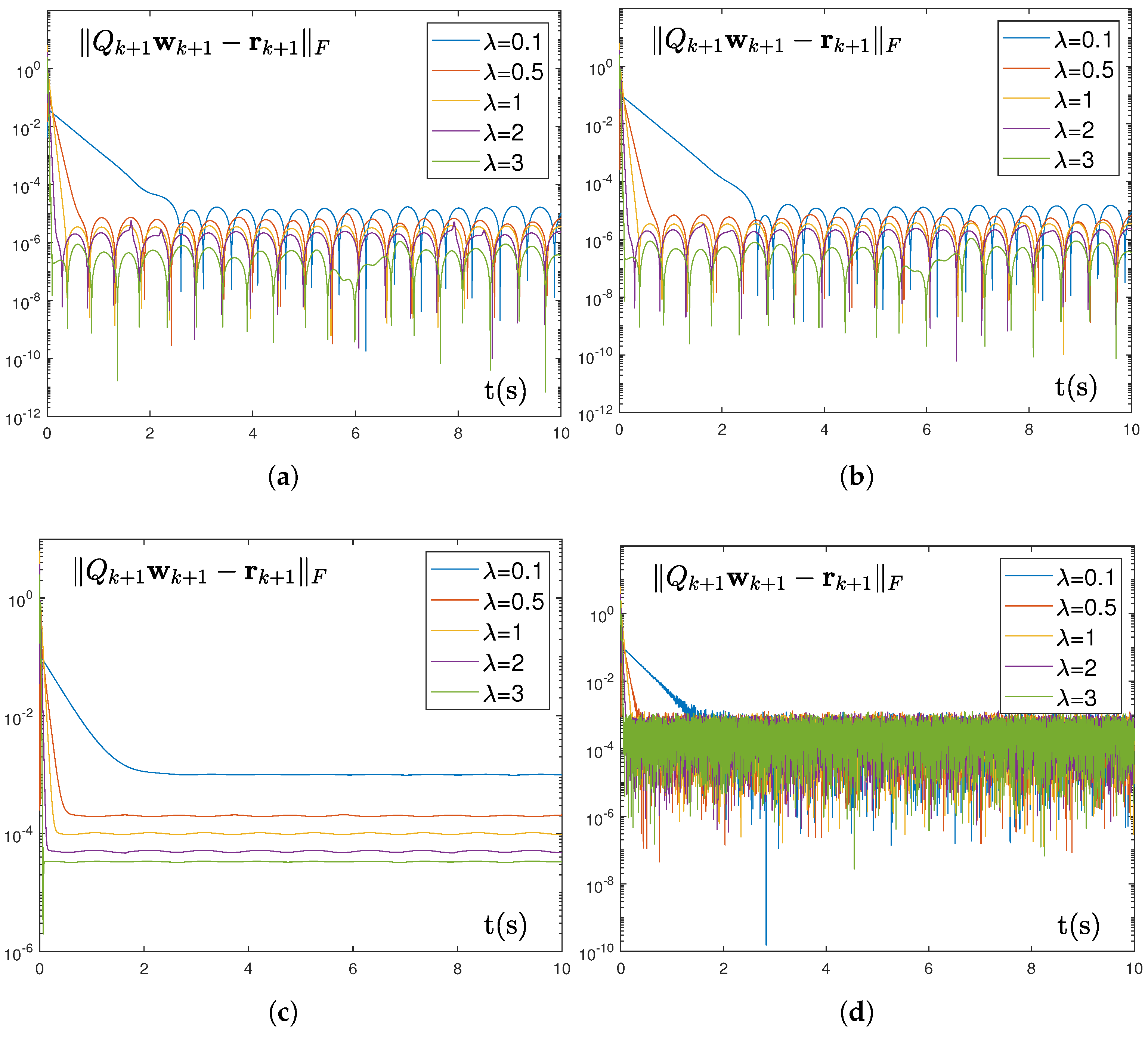
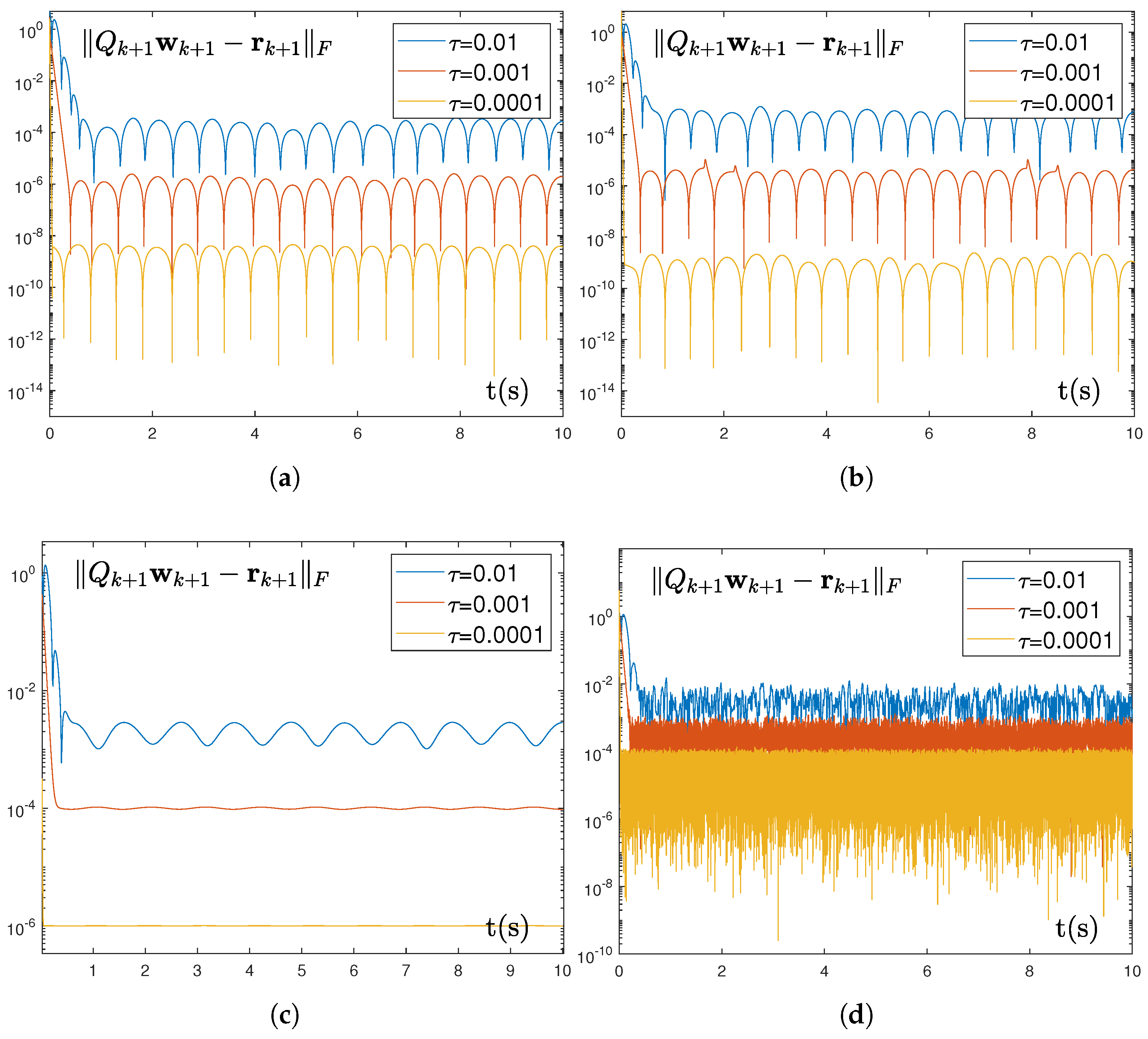
The experimental results of the TD-IRNN model (12) for solving discrete time-varying linear matrix problem with boundary constraints (24) are shown in Figure 2, Figure 3 and Figure 4. As shown in Figure 2, x i (i = 1, 2, 3) denotes the ith element of the feasible solution vector x. It can be seen that the solutions always remain within the constraint range [ x , x + ] under various noise environments, which indicates that the TD-IRNN model (12) can still accurately solve discrete time-varying linear matrix problem with boundary constraints (24) under different noise interferences. In addition, Figure 3 illustrates the residual errors of the TD-IRNN model (12) under different values of integral parameter λ and noise conditions. It can be seen that within the valid range of λ , the model is noise-resistant under all types of noise. Meanwhile, Table 2 presents the mean squared error of the TD-IRNN model (12) under different λ and noise conditions. For λ > 1 , the performance of the TD-IRNN model (12) gradually improves with the increase of λ , and the noise-resistant advantage of the integral term is increasingly manifested. Figure 4 and Table 3 illustrate the residual errors | | Q k + 1 w k + 1 r k + 1 | | F (with | | | | F as the Frobenius norm) of the TD-IRNN model (12) under different noise environments and sampling intervals τ . Specifically, the residual errors converge rapidly in all noise scenarios. Moreover, under different values of τ , the residual errors vary in the form of O ( τ 2 ) , which is consistent with the theoretical analysis results. Based on the above experimental results, it can be proven that the TD-IRNN model (12) is capable of effectively solving discrete time-varying linear matrix problem with boundary constraints (1).
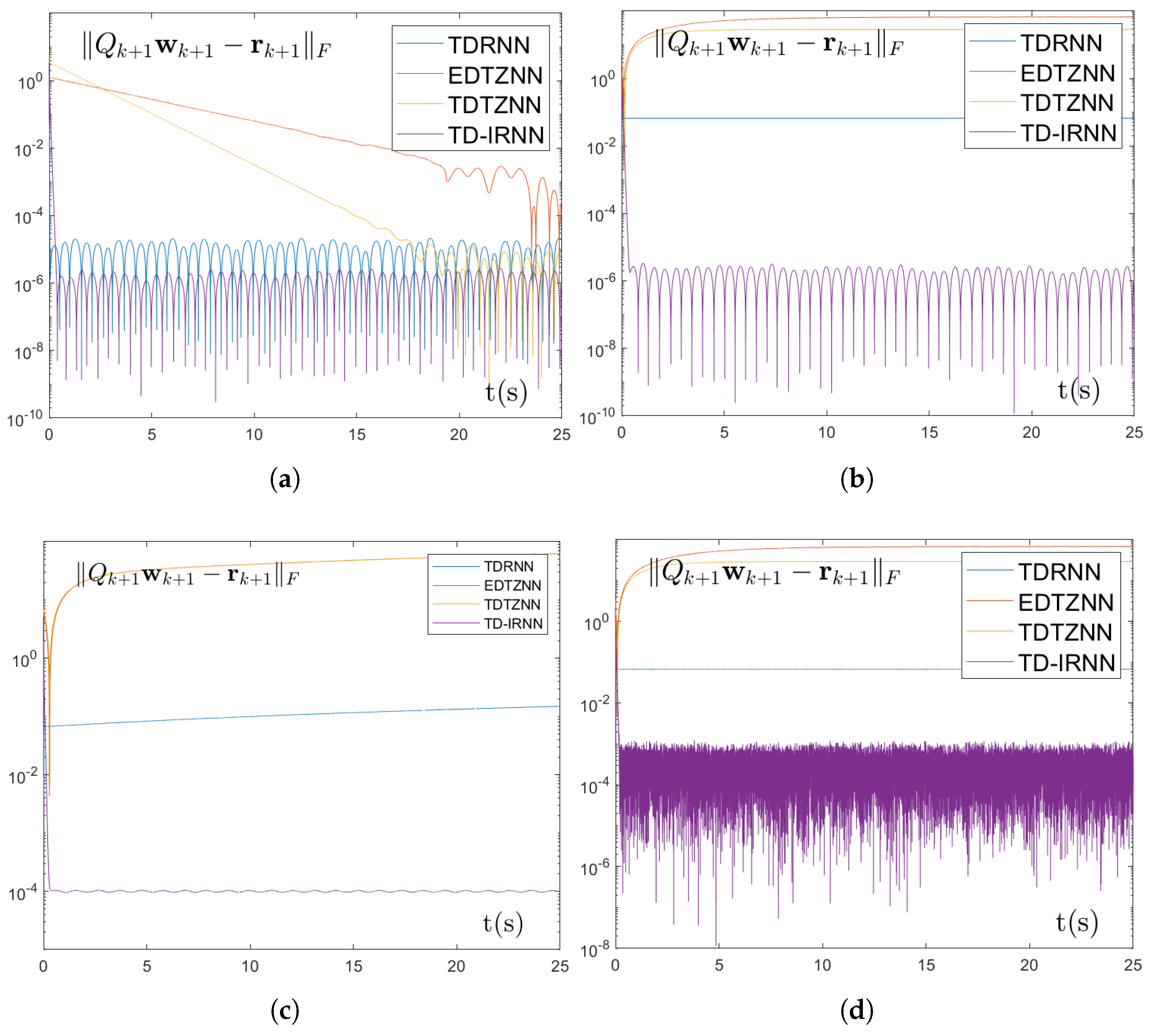
To further verify the superiority of the TD-IRNN model (12), we introduce three different discrete models (i.e., EDTZNN (4), TDTZNN (6), and TDRNN (7) models) for comparison. To clearly present the residual error convergence of each model, the task duration T is set to 25 s. The results of the comparative experiments are shown in Figure 5 and Table 4. Specifically, Figure 5a shows that in the noiseless scenario, all four models can effectively solve the discrete time-varying linear matrix problem with boundary constraints (24), but the convergence rates of the EDTZNN (4) and TDTZNN (6) models are relatively slow, and the convergence precision of the TDRNN (7), EDTZNN (4), and TDTZNN (6) models are all lower than those of the proposed TD-IRNN model (12). In addition, Figure 5b–d show the residual error convergence of each model under different noise environments. It can be seen that only the TD-IRNN model (12) can resist noise interference. The results of the comparative experiments further prove the feasibility and superiority of the TD-IRNN model (12) in solving discrete time-varying linear matrix problem with boundary constraints (1).

5.2. Application of Robotic Arm

This section introduces the application of the proposed TD-IRNN model (12) on a robotic arm with joint physical constraints to demonstrate its applicability and noise resistance.
The motion tracking of a robotic arm includes real-time generation of joint trajectories θ ( t ) R n , and accurate adherence to the expected Cartesian path r ( t ) R m of the end effector. Especially, considering the limitations of feedback and joints, the trajectory tracking of the robotic arm is achieved by effectively solving discrete time-varying linear matrix equations with the following symmetric boundary constraints:
J ( θ ( t ) ) θ ˙ = r ˙ ( t ) k ( ϕ ( θ ( t ) ) r ( t ) ) , θ ˙ θ ˙ ( t ) θ ˙ + , θ θ ( t ) θ + .
The above equation involves several key variables, including the Jacobian matrix J ( θ ( t ) ) R m × n , joint velocity θ ˙ ( t ) , feedback parameter k > 0 R , and differentiable nonlinear mapping function ϕ ( · ) . In addition, θ ˙ ± and θ ± represent the boundary constraints on θ ˙ ( t ) and θ ( t ) , respectively. It should be noted that the method of transforming from (1) to (2) is a general method and does not require symmetry. Therefore, in this experiment, the velocity constraints θ ˙ ± are set to be symmetric for simplicity. The TD-IRNN model (12) is equally applicable to scenarios where both θ and θ ˙ have fully asymmetric constraints. Based on this, achieving the total trajectory of the robotic arm is equivalent to solving the discrete time-varying matrix problem, with the following correlation coefficients:
A ( t ) = J ( θ ( t ) ) b ( t ) = r ˙ ( t ) k ( ϕ ( θ ( t ) ) r ( t ) ) x ( t ) = θ ˙ ( t ) .
In the simulation experiments, we tracked an expected path (i.e., Rhodonea path) using the PUMA560 robotic arm manufactured by UNIMATION Incorporated of the United States (Danbury, CT, USA). To verify the effectiveness and noise resistance of the proposed TD-IRNN model (12), the constraints of PUMA560 robotic arm are defined as
θ ˙ + = θ ˙ = 0.8 ; 0.8 ; 0.8 ; 0.8 ; 0.8 ; 0.8 rad / s θ + = 2.7754 ; 0.7506 ; 3.9274 ; 2.9674 ; 1.7455 ; 4.6256 rad θ = 2.7754 ; 3.8925 ; 0.7855 ; 1.9201 ; 1.7455 ; 4.6256 rad .
The end effector position vectors of the tracked Rhodonea path are designed as
r p = r x r y r z = r cos ( 2 ϕ ) cos ( ϕ ) r + i x 0 r cos ( 2 ϕ ) sin ( ϕ ) cos ( a ) + i y 0 r cos ( 2 ϕ ) sin ( ϕ ) sin ( a ) + i z 0 .
Among them, ϕ = 2 π sin 2 ( π / 2 T ) , time t [ 0 , T ] where T = 10 , parameter a is a constant, and r = 0.26 is the radius of the expected path. In addition, i x 0 , i y 0 , and i z 0 represent the x-axis, y-axis, and z-axis components of the initial position vector of the end vector, respectively.
In the symmetrical flower-shaped path tracking experiment, we set the convergence parameter ω = 0.7 , the design parameter λ = 3 , and the sampling gap τ = 0.001 . Meanwhile, three types of noise disturbances were designed: constant noise as a vector with all elements set to 20, linear noise in the form of 20 + t k , and bounded random noise as a vector with elements randomly fluctuating within the range of 19 to 21, to comprehensively evaluate the noise resistance capability of the TD-IRNN model (12). The experimental results of the robotic arm tracking task are shown in Figure 6 and Figure 7. Figure 6a,b demonstrate that, in a noiseless environment, the TD-IRNN model (12) successfully tracked the flower-shaped trajectory with high precision, achieving an accuracy of 10 5 m. Further observation of the robotic arm joint rotation angles presented in Figure 6c shows that θ 4 exhibits a rapid downward trend after t = 5 s. This is a dynamic adjustment to coordinate with the posture correction of other joints, ensuring the overall system motion converges to the target state. Meanwhile, θ 5 rises rapidly to approximately 1 rad around t = 5 s, which is a collaborative response to the adjustment of θ 4 , helping the system complete the final posture calibration. Furthermore, Figure 6c,d demonstrate that the TD-IRNN model (12) effectively constrained both joint angles and joint velocities within the predefined physical limits, thereby ensuring the stability and safety of robotic arm motion.
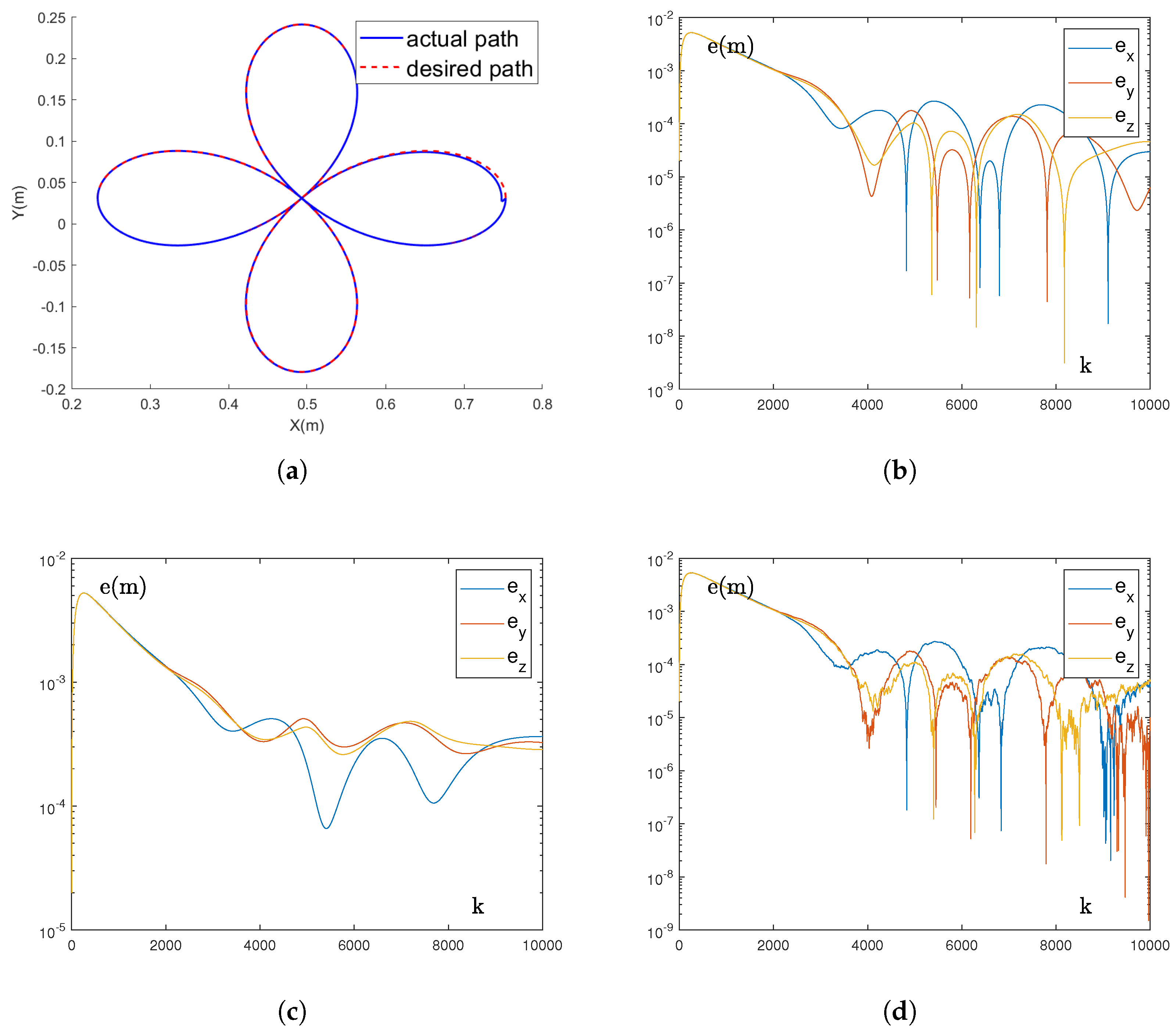
In addition, Figure 7 presents the trajectory tracking results of the robotic arm for the flower-shaped path under various noise interferences. As observed in Figure 7a, even in the presence of noise interferences, the actual path can still coincide with the desired path, completing the trajectory tracking task excellently. Meanwhile, Figure 7b–d show that under the interferences of constant noise, linear noise, and bounded random noise, the maximum position errors of the x, y, and z axes are all of the order of 10 4 m. These results fully demonstrate that the TD-IRNN model (12) exhibits strong noise robustness and can effectively solve practical application problems with noise interferences.

6. Discussion

The TD-IRNN model (12) deals with linear matrix problems with symmetric constraints. In future research, the framework can be extended to nonlinear systems and complex constraints. Specifically, it can be applied to time-varying nonlinear equations through iterative linearization. Using Newton-Raphson steps, the nonlinear problem is approximated as a sequence of discrete time-varying linear matrix problems at each time step k. The TD-IRNN model is then employed to efficiently solve the increment of each linearized subproblem, thereby driving the overall solution toward the root of the nonlinear system. For complex constraints such as polyhedral constraints, ideas similar to the active set or interior-point methods can be utilized. The TD-IRNN is designed to solve the optimality conditions derived from the KKT conditions, and these conditions themselves constitute a linear or linearized system. These extensions demonstrate the great potential of the direct discrete-time integral recurrent neural network method for addressing a broad range of dynamic optimization and control problems.

7. Conclusions

This article proposes a Taylor-type direct-discrete-time integral noise-immune recurrent neural network (TD-IRNN) model for solving the discrete time-varying linear matrix problem with boundary constraints. Firstly, the TD-IRNN model (12) solves the problem directly in the discrete domain without the need for transformation to a continuous environment, thereby improving computational efficiency and practicality. In addition, an integral term is incorporated during the model construction process, effectively enhancing the noise resistance of the TD-IRNN model (12). Secondly, this paper systematically analyzes the convergence and robustness of the TD-IRNN model (12) under both noise-free and noise injection scenarios, confirming its stable performance under various interference conditions. Furthermore, numerical experiments and robotic arm trajectory tracking experiments validate the applicability and reliability of the TD-IRNN model (12) in complex noisy environments. The results confirm that the TD-IRNN model (12) not only achieves higher accuracy and faster convergence than the other three models in noise-free scenarios but also maintains excellent tracking precision under significant noise interference, highlighting its practical value. In conclusion, the TD-IRNN model establishes an efficient, robust, and practical framework for solving constrained time-varying problems in discrete-time settings, providing new ideas and methods for research and application in related fields.

Author Contributions

Conceptualization, C.Y.; methodology, Y.C.; software, Y.C.; validation, X.L.; formal analysis, X.L.; investigation, X.L.; resources, C.Y.; data curation, Y.L.; writing—original draft preparation, X.L. and Y.C.; writing—review and editing, J.C.; visualization, X.L.; supervision, C.Y.; project administration, Y.C.; funding acquisition, C.Y. All authors have read and agreed to the published version of the manuscript.

Funding

This work was supported by Guangdong basic and applied basic research foundation under Grant (2025A1515010466), Guangdong Key Construction Discipline Scientific Research Ability Enhancement Project (2024ZDJS056) and the Guangzhou Programs (2024312151, 2024312000 and 2024312374). National Natural Science Foundation of China (11561029).

Data Availability Statement

The original contributions presented in this study are included in the article material. Further inquiries can be directed to the corresponding author.

Conflicts of Interest

The authors declare no conflicts of interest.

References

  1. Zhang, T.; Xu, S.; Zhang, W. New Approach to Feedback Stabilization of Linear Discrete Time-Varying Stochastic Systems. IEEE Trans. Autom. Control 2025, 70, 2004–2011. [Google Scholar] [CrossRef]
  2. Cui, Y.; Song, Z.; Wu, K.; Yan, J.; Chen, C.; Zhu, D. A Discrete-Time Neurodynamics Scheme for Time-Varying Nonlinear Optimization with Equation Constraints and Application to Acoustic Source Localization. Symmetry 2025, 17, 932. [Google Scholar] [CrossRef]
  3. Chen, Y.; Chen, J.; Yi, C. A pre-defined finite time neural solver for the time-variant matrix equation E (t) X (t) G (t) = D (t). J. Frankl. Inst. 2024, 361, 106710. [Google Scholar] [CrossRef]
  4. Zhou, B.; Dong, J.; Cai, G. Normal Forms of Linear Time-Varying Systems with Applications to Output-Feedback Stabilization and Tracking. IEEE Trans. Cybern. 2025, 55, 2671–2683. [Google Scholar] [CrossRef]
  5. Hu, K.; Liu, T. Robust Data-Driven Predictive Control for Linear Time-Varying Systems. IEEE Control Syst. Lett. 2024, 8, 910–915. [Google Scholar] [CrossRef]
  6. Tang, W.; Cai, H.; Xiao, L.; He, Y.; Li, L.; Zuo, Q.; Li, J. A Predefined-Time Adaptive Zeroing Neural Network for Solving Time-Varying Linear Equations and Its Application to UR5 Robot. IEEE Trans. Neural Netw. Learn. Syst. 2025, 36, 4703–4712. [Google Scholar] [CrossRef]
  7. Zhang, X.; Peng, Y.; Luo, B.; Pan, W.; Xu, X.; Xie, H. Model-based safe reinforcement learning with time-varying constraints: Applications to Intelligent vehicles. IEEE Trans. Ind. Electron. 2024, 71, 12744–12753. [Google Scholar] [CrossRef]
  8. Han, F.; Wang, Z.; Liu, H.; Dong, H.; Lu, G. Local Design of Distributed State Estimators for Linear Discrete Time-Varying Systems Over Binary Sensor Networks: A Set-Membership Approach. IEEE Trans. Syst. Man Cybern. Syst. 2024, 54, 5641–5654. [Google Scholar] [CrossRef]
  9. Wang, Z.; Ma, Y.; Zhang, Q.; Tang, W.; Shen, Y. Interval Estimation for Time-Varying Descriptor Systems via Simultaneous Optimizations of Multiple Interval Widths. IEEE Trans. Syst. Man Cybern. Syst. 2024, 54, 3774–3782. [Google Scholar] [CrossRef]
  10. Liu, Q.; Yue, Y. Distributed Multiagent System for Time-Varying Quadratic Programming with Application to Target Encirclement of Multirobot System. IEEE Trans. Syst. Man Cybern. Syst. 2024, 54, 5339–5351. [Google Scholar] [CrossRef]
  11. Tang, Z.; Zhang, Y.; Ming, L. Novel Snap-Layer MMPC Scheme via Neural Dynamics Equivalency and Solver for Redundant Robot Arms with Five-Layer Physical Limits. IEEE Trans. Neural Netw. Learn. Syst. 2025, 36, 3534–3546. [Google Scholar] [CrossRef]
  12. Lei, Y.; Xu, L.; Chen, J. Parameter-Gain Accelerated ZNN Model for Solving Time-Variant Nonlinear Inequality-Equation Systems and Application on Tracking Symmetrical Trajectory. Symmetry 2025, 17, 1342. [Google Scholar] [CrossRef]
  13. Chen, G.; Du, G.; Xia, J.; Xie, X.; Wang, Z. Aperiodic Sampled-Data H Control of Vehicle Active Suspension System: An Uncertain Discrete-Time Model Approach. IEEE Trans. Ind. Inform. 2024, 20, 6739–6750. [Google Scholar] [CrossRef]
  14. Yang, H.; Yang, L.; Ivanov, I.G. Controller Design for Continuous-Time Linear Control Systems with Time-Varying Delay. Mathematics 2025, 13, 2519. [Google Scholar] [CrossRef]
  15. Liufu, Y.; Jin, L.; Li, S. Adaptive Noise-Learning Differential Neural Solution for Time-Dependent Equality-Constrained Quadratic Optimization. IEEE Trans. Neural Netw. Learn. Syst. 2025, 36, 17253–17264. [Google Scholar] [CrossRef]
  16. Lin, C.; Jiang, Z.; Cong, J.; Zou, L. RNN with High Precision and Noise Immunity: A Robust and Learning-Free Method for Beamforming. IEEE Internet Things J. 2025, 12, 15779–15791. [Google Scholar] [CrossRef]
  17. Tan, J.; Shang, M.; Jin, L. Metaheuristic-Based RNN for Manipulability Optimization of Redundant Manipulators. IEEE Trans. Ind. Inform. 2024, 20, 6489–6498. [Google Scholar] [CrossRef]
  18. Li, X.; Lin, F.; Wang, H.; Zhang, X.; Ma, H.; Wen, C.; Blaabjerg, F. Temporal Modeling for Power Converters with Physics-in-Architecture Recurrent Neural Network. IEEE Trans. Ind. Electron. 2024, 71, 14111–14123. [Google Scholar] [CrossRef]
  19. Abdul Aziz, M.; Rahman, M.H.; Abrar Shakil Sejan, M.; Tabassum, R.; Hwang, D.D.; Song, H.K. Deep Recurrent Neural Network Based Detector for OFDM with Index Modulation. IEEE Access 2024, 12, 89538–89547. [Google Scholar] [CrossRef]
  20. Cai, J.; Zhang, W.; Zhong, S.; Yi, C. A super-twisting algorithm combined zeroing neural network with noise tolerance and finite-time convergence for solving time-variant Sylvester equation. Expert Syst. Appl. 2024, 248, 123380. [Google Scholar] [CrossRef]
  21. Zhang, Y.; Yi, C. Zhang Neural Networks and Neural-Dynamic Method; Nova Science Publishers, Inc.: Hauppauge, NY, USA, 2011. [Google Scholar]
  22. Seo, J.H.; Kim, K.D. An RNN-Based Adaptive Hybrid Time Series Forecasting Model for Driving Data Prediction. IEEE Access 2025, 13, 54177–54191. [Google Scholar] [CrossRef]
  23. Zheng, B.; Li, C.; Zhang, Z.; Yu, J.; Liu, P.X. An Arbitrarily Predefined-Time Convergent RNN for Dynamic LMVE with Its Applications in UR3 Robotic Arm Control and Multiagent Systems. IEEE Trans. Cybern. 2025, 55, 1789–1800. [Google Scholar] [CrossRef] [PubMed]
  24. Xu, F.; Li, Z.; Nie, Z.; Shao, H.; Guo, D. New recurrent neural network for online solution of time-dependent underdetermined linear system with bound constraint. IEEE Trans. Ind. Inform. 2018, 15, 2167–2176. [Google Scholar] [CrossRef]
  25. Shi, Y.; Chong, W.; Cao, X.; Jiang, C.; Zhao, R.; Gerontitis, D.K. A New Double-Integration-Enhanced RNN Algorithm for Discrete Time-Variant Equation Systems with Robot Manipulator Applications. IEEE Trans. Autom. Sci. Eng. 2025, 22, 8856–8869. [Google Scholar] [CrossRef]
  26. Li, J.; Pan, S.; Chen, K.; Zhu, X.; Yang, M. Inverse-Free discrete ZNN models for solving future nonlinear equality and inequality system with robot manipulator control. IEEE Trans. Ind. Electron. 2025. Early Access. [Google Scholar] [CrossRef]
  27. Cang, N.; Qiu, F.; Xue, S.; Jia, Z.; Guo, D.; Zhang, Z.; Li, W. New discrete-time zeroing neural network for solving time-dependent linear equation with boundary constraint. Artif. Intell. Rev. 2024, 57, 140. [Google Scholar] [CrossRef]
  28. Jin, L.; Zhang, Y.; Li, S.; Zhang, Y. Modified ZNN for time-varying quadratic programming with inherent tolerance to noises and its application to kinematic redundancy resolution of robot manipulators. IEEE Trans. Ind. Electron. 2016, 63, 6978–6988. [Google Scholar] [CrossRef]
  29. Zheng, L.; Yu, W.; Xu, Z.; Zhang, Z.; Deng, F. Design, Analysis, and Application of a Discrete Error Redefinition Neural Network for Time-Varying Quadratic Programming. IEEE Trans. Neural Netw. Learn. Syst. 2024, 35, 13646–13657. [Google Scholar] [CrossRef]
  30. Shi, Y.; Sheng, W.; Wang, J.; Jin, L.; Li, B.; Sun, X. Real-Time Tracking Control and Efficiency Analyses for Stewart Platform Based on Discrete-Time Recurrent Neural Network. IEEE Trans. Syst. Man Cybern. Syst. 2024, 54, 5099–5111. [Google Scholar] [CrossRef]
  31. Shi, Y.; Ding, C.; Li, S.; Li, B.; Sun, X. Discrete generalized-Sylvester matrix equation solved by RNN with a novel direct discretization numerical method. Numer. Algorithms 2023, 93, 971–992. [Google Scholar] [CrossRef]
  32. Lu, H.; Jin, L.; Luo, X.; Liao, B.; Guo, D.; Xiao, L. RNN for solving perturbed time-varying underdetermined linear system with double bound limits on residual errors and state variables. IEEE Trans. Ind. Inform. 2019, 15, 5931–5942. [Google Scholar] [CrossRef]
  33. Shi, Y.; Ding, C.; Li, S.; Li, B.; Sun, X. New RNN Algorithms for Different Time-Variant Matrix Inequalities Solving Under Discrete-Time Framework. IEEE Trans. Neural Netw. Learn. Syst. 2025, 36, 5244–5257. [Google Scholar] [CrossRef]
  34. Shi, Y.; Chong, W.; Zhao, W.; Li, S.; Li, B.; Sun, X. A new recurrent neural network based on direct discretization method for solving discrete time-variant matrix inversion with application. Inf. Sci. 2024, 652, 119729. [Google Scholar] [CrossRef]
  35. Hu, Y.; Zhang, C.; Wang, B.; Zhao, J.; Gong, X.; Gao, J.; Chen, H. Noise-tolerant znn-based data-driven iterative learning control for discrete nonaffine nonlinear mimo repetitive systems. IEEE/CAA J. Autom. Sin. 2024, 11, 344–361. [Google Scholar] [CrossRef]
  36. Huang, S.; Ma, Z.; Yu, S.; Han, Y. New discrete-time zeroing neural network for solving time-variant underdetermined nonlinear systems under bound constraint. Neurocomputing 2022, 487, 214–227. [Google Scholar] [CrossRef]
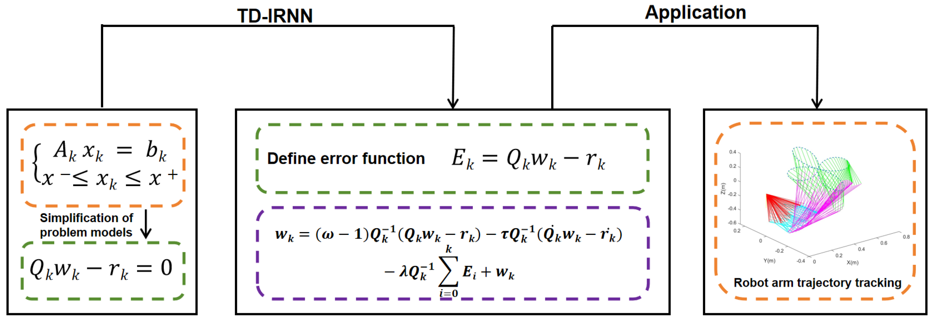
Figure 1. TD-IRNN model framework diagram.
Symmetry 17 01975 g001
Figure 2. State trajectories obtained by the proposed TD-IRNN model (12) for solving discrete time-varying linear matrix problem with boundary constraints (24) under different noise interferences, with parameters τ = 0.001 , ω = 0.7 , and λ = 1 . The red dotted line in the figure indicates the constraint range [ x , x + ] . (a) The state trajectories starting from five randomly generated initial values under the noiseless condition. (b) The state trajectories under constant noise, linear noise, and bounded random noise. The three blue lines under each type of noise represent x i .
Symmetry 17 01975 g002
Figure 3. Residual errors of the TD-IRNN model (12) in solving discrete time-varying linear matrix problem with boundary constraints (24) with different integral parameter λ and noise conditions. (a) No noise. (b) Constant noise. (c) Linear noise. (d) Bounded random noise.
Symmetry 17 01975 g003
Figure 4. Residual errors of the TD-IRNN model (12) in solving discrete time-varying linear matrix problem with boundary constraints (24) with different τ and different noise interferences. (a) No noise. (b) Constant noise. (c) Linear noise. (d) Bounded random noise.
Symmetry 17 01975 g004
Figure 5. Compare the residual errors of EDTZNN (4), TDTZNN (6), TDRNN (7), and TD-IRNN (12) models in solving discrete time-varying linear matrix problem with boundary constraints (24) under different noises. (a) No noise. (b) Constant noise. (c) Linear noise. (d) Bounded random noise.
Symmetry 17 01975 g005
Figure 6. Simulation results of the PUMA560 robotic arm tracking a flower-shaped trajectory using the TD-IRNN model (12) in a noiseless environment with parameters λ = 3 , ω = 0.7 , and τ = 0.001 . (a) Robot arm trajectory. (b) Position errors of the end-effector in the X, Y, and Z axes. (c) Joint rotation angle of robotic arm. (d) Rotation speed of robotic arm joints.
Symmetry 17 01975 g006
Figure 7. Experimental results of the PUMA560 robotic arm tracking a flower-shaped path under different noise interferences with parameters λ = 3 , ω = 0.7 , and τ = 0.001 . (a) Desired path and actual path. (b) Position errors of the end-effector in the X, Y, and Z axes under constant noise. (c) Position errors of the end-effector in the X, Y, and Z axes under linear noise. (d) Position errors of the end-effector in the X, Y, and Z axes under bounded random noise.
Symmetry 17 01975 g007
Table 1. Comparative summary of different discrete models for solving discrete time-varying linear matrix problems with boundary constraints.
ModelConstruction ParadigmCore Mechanism for Noise Robustness
EDTZNNcontinuous-time discretization (Euler)none (highly susceptible to noise)
TDTZNNcontinuous-time discretization (Taylor)none (highly susceptible to noise)
TDRNNdirect-discrete-timenone (susceptible to noise)
TD-IRNN (This work)direct discrete-timeintegral-enhanced error dynamics
Table 2. Mean Squared Error of TD-IRNN Model (12) Under Different Integral Parameter λ and Noise Conditions In The Numerical Experiment (24) with ω = 0.7 .
Integral Parameter λ Different NoisesMean Squared Error
0.1No noise 1.1174 × 10 3
linear noise 1.2540 × 10 3
random noise 1.2552 × 10 3
constant noise 1.2498 × 10 3
0.5No noise 9.2920 × 10 3
linear noise 1.0013 × 10 3
random noise 1.0035 × 10 3
constant noise 1.001 × 10 3
1No noise 9.0476 × 10 3
linear noise 9.2311 × 10 3
random noise 9.236 × 10 3
constant noise 9.2308 × 10 3
2No noise 3.5511 × 10 3
linear noise 3.6589 × 10 3
random noise 3.6619 × 10 3
constant noise 3.6588 × 10 3
3No noise 1.7786 × 10 3
linear noise 1.8510 × 10 3
random noise 1.8531 × 10 3
constant noise 1.8509 × 10 3
Table 3. Residual Errors of TD-IRNN Model (12) Under Different Values of Sampling Gap τ and Noise Conditions in the Numerical Experiment (24).
Sampling Gap τ Different NoisesSteady-State Error
0.01linear noise 1.9692 × 10 3
random noise 4.1177 × 10 3
constant noise 7.2168 × 10 4
0.001linear noise 1.0242 × 10 4
random noise 5.7189 × 10 4
constant noise 2.7232 × 10 6
0.0001linear noise 1.0038 × 10 6
random noise 3.4793 × 10 5
constant noise 3.7936 × 10 9
Table 4. Comparison of the Residual Errors Among The EDTZNN (4), TDTZNN (6), TDRNN (7), and TD-IRNN (12) Models Under Different Types of Noise in the Numerical Experiment (24).
CNLNRBN
EDTZNN model 64.669 103.165 67.8249
TDTZNN model 28.5705 48.5804 29.2829
TDRNN model6.6655 × 10 2 1.1398 × 10 1 6.8604 × 10 2
TD-IRNN model2.0715 × 10 6 1.002 × 10 4 7.5244 × 10 4
CN, LN, and RBN denote constant noise 20, linear noise 20 + t k , and bounded random noise between 19 and 21, respectively.
Disclaimer/Publisher’s Note: The statements, opinions and data contained in all publications are solely those of the individual author(s) and contributor(s) and not of MDPI and/or the editor(s). MDPI and/or the editor(s) disclaim responsibility for any injury to people or property resulting from any ideas, methods, instructions or products referred to in the content.