Article

A Derivative-Free Method with the Symmetric Rank-One Update for Constrained Nonlinear Systems of Monotone Equations

Department of Mathematics, Huzhou University, Huzhou 313000, China
Symmetry 2025, 17(11), 1956; https://doi.org/10.3390/sym17111956
Submission received: 11 October 2025 / Revised: 4 November 2025 / Accepted: 6 November 2025 / Published: 14 November 2025
(This article belongs to the Section Mathematics)

Abstract

This paper presents a new derivative-free method with a symmetric rank-one (SR1) update for handling constrained nonlinear systems of monotone equations. Distinctively, the approach employs a revised SR1 update formula that leverages information from the latest three iterates and their corresponding function values—a key improvement over existing SR1 variants relying only on two-point information. Derived from this revised formula, the approach integrates projection techniques for performance enhancement. One of its key advantages lies in the search direction: it exhibits sufficient descent and trust-region properties while eliminating the need for line search techniques. Theoretical analysis shows that the algorithm converges globally under specified conditions. Furthermore, numerical experiments are conducted to compare the proposed algorithm with two other existing approaches; results demonstrate that it exhibits superior reliability and robustness in terms of the number of iterations, function evaluations, and CPU runtime.

1. Introduction

This paper focuses on solving the constrained system of nonlinear equations formulated as follows:
F ( x ) = 0 , x Ω ,
where F : R n R n denotes a monotone and continuously differentiable mapping, and Ω R n represents a nonempty closed convex set.
Formally, the monotonicity of the mapping F is characterized by the following inequality:
( F ( x ) F ( y ) ) T ( x y ) 0 , x , y R n .
Systems of nonlinear monotone equations originate from numerous practical problems and are widely applied in interdisciplinary fields. Typical application scenarios include automatic control systems [1], optimal power flow calculations [2], and compressive sensing [3,4,5]. Given the broad scope of application fields for nonlinear monotone equations, a multitude of researchers have developed an array of iterative numerical techniques to solve Problem (1). Examples of such methods include the Newton algorithm [6], the Gauss–Newton algorithm [7], the BFGS algorithm [8], the quasi-Newton algorithm [9], and gradient-based algorithms [10,11,12,13].
In recent years, several optimization methods, which were developed based on the projection and proximal point approach initially proposed by Solodov and Svaiter [14], have been extended to tackle Problem (1). Among these extended approaches are conjugate gradient methods—originally developed for solving large-scale unconstrained optimization problems, owing to their advantages of low memory requirements and a simple structural design. For instance, Li and Zheng [15] developed two derivative-free approaches for solving nonlinear monotone equations. Dai and Zhu [16] integrated a projection technique into the modified HS conjugate gradient approach and proposed a derivative-free projection approach to tackle high-dimensional nonlinear monotonic equations. Additionally, Kimiaei et al. [17] established a subspace inertial algorithm specifically tailored for derivative-free nonlinear monotone equations. Meanwhile, Liu et al. [18] developed an accelerated Dai-Yuan conjugate gradient projection approach, which incorporates an optimal parameter selection strategy to enhance performance. P.Kumam et al. [19] proposed another hybrid approach for solving monotone operator equations and applied it to signal processing problems. Xia et al. [20] proposed a modified two-term conjugate gradient-based projection algorithm for constrained nonlinear equations. Fang [21] presented a derivative-free RMIL conjugate gradient approach for constrained nonlinear systems of monotone equations. Zhang et al. [22] developed a three-term projection approach specifically formulated for solving nonlinear monotone equations, with subsequent extension of this approach to address practical problems in signal processing, thereby validating its applicability.
Another class of widely used iterative methods for solving nonlinear equations is the quasi-Newton approach. For example, Abubakar et al. [23] proposed a scaled memoryless quasi-Newton approach based on the SR1 update formula for solving systems of nonlinear monotone operator equations. Awwal et al. [24] proposed a new derivative-free spectral projection approach for addressing Problem (1), with the aid of a modified SR1 updating formula. Rao and Huang [25] developed a novel sufficient descent direction based on a scaled memoryless DFP updating formula and proposed a derivative-free approach for solving systems of nonlinear monotone equations. Tang and Zhou [26] proposed a two-step Broyden-like approach for solving nonlinear equations, which is designed to compute an additional approximate quasi-Newton step formed by using the previous Broyden-like matrix when the iterates are close to the solution set. Ullah et al. [27] introduces a two-parameter scaled memoryless BFGS approach with scaling for solving systems of monotone nonlinear equations, in which the optimal scaling parameters are determined by minimizing a measure function that incorporates all eigenvalues of the memoryless BFGS matrix.
Inspired by the studies mentioned above, a new quasi-Newton method is proposed in this paper for solving nonlinear equations, with a revised SR1 updating formula as its technical support. The proposed approach in this paper has the following advantages: (1) The search direction is constructed based on the revised SR1 update formula and utilizes information from the latest three iterates ( x k 2 , x k 1 , x k ) and their corresponding function values. This three-point information captures richer curvature characteristics, outperforming two-point approaches by enhancing direction reliability. (2) Under the framework of the Lipschitz condition and convex constraints, this approach demonstrates global convergence when applied to monotone nonlinear equations. (3) The search direction of our proposed approach possesses the properties of both sufficient descent and the trust region, with no reliance on line search techniques.
The remainder of this paper is structured as follows: Section 2 elaborates on the motivation behind the proposed approach and presents the corresponding algorithm. Section 3 analyzes the global convergence of the proposed approach. Section 4 conducts comparative numerical experiments to evaluate the method’s performance. Section 5 provides a summary.

2. Algorithm

In this section, we first revisit the quasi-Newton iterative methods, which produce { x k } using the following iterative formula:
x k + 1 = x k + α k d k .
Within this framework, the step length α k is obtained using line search methods, and the search direction d k is computed based on
d k = M k F ( x k ) ,
in which M k is an approximation of the inverse of the Hessian matrix at the k-th iteration. One well-known quasi-Newton matrix update formula, specifically the Symmetric Rank-One (SR1) approach, is presented as follows:
M k = M k 1 + ( s k 1 M k 1 y k 1 ) ( s k 1 M k 1 y k 1 ) T ( s k 1 M k 1 y k 1 ) T y k 1 ,
where s k 1 = x k x k 1 , y k 1 = F ( x k ) F ( x k 1 ) . In the iterative process of the SR1 approach, the iterative matrix M k can hardly maintain positive definiteness consistently. Meanwhile, the denominator may tend to zero, resulting in the failure of the algorithm.
To enhance the performance of the original SR1 approach, two modified formulations have been proposed in existing studies. One is by Abubakar et al. [23], who adjusted (5) to introduce a parameter θ , and the modified formula is given by:
M k = M k 1 + ( s k 1 M k 1 θ y k 1 ) ( s k 1 M k 1 θ y k 1 ) T s k 1 T ( y k 1 + w s k 1 ) .
The other is by Awwal et al. [24], who improved the denominator of (5) using a max function to avoid singularity. Their modified formula reads:
M k = M k 1 + ( s k 1 M k 1 y k 1 ) ( s k 1 M k 1 y k 1 ) T max { s k 1 T ( y k 1 + w s k 1 ) , y k 1 + w s k 1 2 } .
The SR1 improvement formulas (6) and (7) relying only on the latest two points have two key flaws. First, heavy dependence on the recent s k 1 and y k 1 causes information singularity. Limited local data fails to capture the global curvature of the function, leading to inaccurate Hessian inverse approximations and unstable convergence paths—especially in strongly nonlinear problems. Second, they underperform in high-dimensional or tightly constrained scenarios: two vectors cannot fully represent multi-dimensional curvature, and the tiny s k 1 from tight constraints reduces information distinguishability, rendering matrix updates ineffective and causing algorithm stagnation.
In [28], Broyden put forward the following update formula:
B k = B k 1 + ( y k 1 B k 1 s k 1 ) s k 1 T s k 1 T s k 1 T ,
where B k is an approximation of the Jacobian matrix at the k-th iteration. Based on Broyden’s work, Fang et al. [9] proposes a modified quasi-Newton method, whose update formula is
B k = B k 1 + ( y ¯ k 1 B k 1 s ¯ k 1 ) s ¯ k 1 T s ¯ k 1 T s ¯ k 1 T ,
where s ¯ k 1 = s k 1 δ k 1 s k 2 , y ¯ k 1 = y k 1 δ k 1 y k 2 , δ k 1 = s k 1 2 s k 2 ( 2 s k 1 + s k 2 ) .
Numerical experiments indicate that the modified quasi-Newton method holds considerable promise. Inspired by Equation (9), this paper proposes a revised SR1 update formula as follows:
M k = μ k M k 1 + ( s k 1 M k 1 y k 1 ) ( s k 1 M k 1 y k 1 ) T ( s ˜ k 1 M k 1 y ˜ k 1 ) T y ˜ k 1 ,
where μ k > 0 , s ˜ k 1 = s k 1 δ k 1 s k 2 + t k 1 y ˜ k 1 , y ˜ k 1 = y k 1 δ k 1 y k 2 , δ k 1 = s k 1 2 s k 2 ( 2 s k 1 + s k 2 ) , t k 1 = 1 + F k 1 2 + δ k 1 ( s k 1 T y k 2 + s k 2 T y k 1 ) y ˜ k 1 2 . If we set μ k = 1 , δ k 1 = 0 , t k 1 = 0 for all k, then the SR1 update given by (10) reduces to the classical version.
According to the definitions of  s ˜ k 1  and  y ˜ k 1 , we have
( s ˜ k 1 M k 1 y ˜ k 1 ) T y ˜ k 1 = ( s k 1 δ k 1 s k 2 + t k 1 y ˜ k 1 M k 1 y ˜ k 1 ) T y ˜ k 1 = s k 1 T y ˜ k 1 δ k 1 s k 2 T y ˜ k 1 + t k 1 y ˜ k 1 T y ˜ k 1 y ˜ k 1 T M k 1 y ˜ k 1 = s k 1 T ( y k 1 δ k 1 y k 2 ) δ k 1 s k 2 T ( y k 1 δ k 1 y k 2 ) + F k 1 2 + δ k 1 ( s k 1 T y k 2 + s k 2 T y k 1 ) + y ˜ k 1 T ( I M k 1 ) y ˜ k 1 = s k 1 T y k 1 + δ k 1 2 s k 2 T y k 2 + F k 1 2 + y ˜ k 1 T ( I M k 1 ) y ˜ k 1 ,
where I is an identity matrix with the same dimension as  M k 1 . If we set M k 1 = I and use (10), we have
M k = μ k I + ( s k 1 y k 1 ) ( s k 1 y k 1 ) T s k 1 T y k 1 + δ k 1 2 s k 2 T y k 2 + F k 1 2 ,
Based on the monotonicity of F and μ k > 0 , we conclude that M k is a symmetric positive definite matrix.
Combining with (4) and (10), we have
d k = F k if k = 0 μ k F k ( s k 1 y k 1 ) ( s k 1 y k 1 ) T F k ( s ˜ k 1 y ˜ k 1 ) T y ˜ k 1 if k 1 .
From the definition of  d k , it is easy to see that for  k N , we have
F k T d k = μ k F k T F k F k T ( s k 1 y k 1 ) ( s k 1 y k 1 ) T F k ( s ˜ k 1 y ˜ k 1 ) T y ˜ k 1 = μ k + F k T ( s k 1 y k 1 ) 2 ( s ˜ k 1 y ˜ k 1 ) T y ˜ k 1 F k 2 F k 2
For c > 0 , we set
μ k = c F k T ( s k 1 y k 1 ) 2 ( s ˜ k 1 y ˜ k 1 ) T y ˜ k 1 F k 2 ,
and then we get F k T d k = c F k 2 . When k = 0 , we have F 0 T d 0 = μ 0 F 0 2 . In addition, inspired by the BB method [29], we propose the following parameter:
λ k = s k 1 T s k 1 s ˜ k 1 T y ˜ k 1 .
Furthermore, using (13), (15) and (16), this paper proposes the modified search direction as follows:
d k = F k if k = 0 max { μ k , λ k } F k β k η k if k 1
where β k = ( s k 1 y k 1 ) T F k ( s ˜ k 1 y ˜ k 1 ) T y ˜ k 1 , η k = s k 1 y k 1 . s ˜ k 1 = s k 1 δ k 1 s k 2 + t k 1 y ˜ k 1 , y ˜ k 1 = y k 1 δ k 1 y k 2 , δ k 1 = s k 1 2 s k 2 ( 2 s k 1 + s k 2 ) , t k 1 = 1 + F k 1 2 + δ k 1 ( s k 1 T y k 2 + s k 2 T y k 1 ) y ˜ k 1 2 .
Next, we introduce the projection operator  P Ω [ · ] , defined as follows:
P Ω [ x ] = arg min { x y y Ω } , x R n .
This operator corresponds to projecting the vector x onto the closed convex set  Ω . Such a projection ensures that the subsequent iterative points generated by our algorithm stay within the domain  Ω . It is well known that the projection operator satisfies the non-expansive property, which is expressed as
P Ω [ x ] P Ω [ y ] x y , x , y R n .
Next, we present the detailed steps of our proposed algorithm (Algorithm 1).
Algorithm 1 Revised SR1 update Method (RSR1M)
  • Step 0 : Select θ > 0 , σ > 0 , ϵ > 0 , ζ 2 > ζ 1 > 0 , 1 > ρ > 0 , 2 > γ > 0 . along with an initial point x 0 R n . Let k = 0 .
  • Step 1 : If F ( x k ) < ϵ , terminate the algorithm; Otherwise, proceed to step 2.
  • Step 2 : Determine the search direction d k via (17).
  • Step 3 : Define the step-length α k = θ ρ m , m is the smallest natural number that makes α k satisfy the following inequality:
    F ( x k + α k d k ) T d k σ α k P [ ζ 1 , ζ 2 ] | | F ( x k + α k d k ) | | · | | d k | | 2 .
  • The definition of the projection operator P for z R is
    P [ ζ 1 , ζ 2 ] [ z ] = ζ 2 if z ζ 2 ζ 1 if z ζ 1 z otherwise .
  • Moreover, set h k = x k + α k d k and proceed to step 4.
  • Step 4 : If h k Ω and F ( h k ) < ϵ , set x k + 1 = h k , terminate the algorithm; Otherwise compute
    x k + 1 = P Ω [ x k γ F ( h k ) T ( x k h k ) F ( h k ) 2 F ( h k ) ]
    and set k : = k + 1 , proceed to step 1.

3. Convergence Analysis

Next, we analyze the convergence of the proposed algorithm. The following assumptions are required:
Assumption 1.
The solution set Ω corresponding to Problem (1) is nonempty.
Assumption 2.
F is Lipschitz continuous on R n , meaning that
| | F ( x 1 ) F ( x 2 ) | | L | | x 1 x 2 | | , x 1 , x 2 R n .
Lemma 1.
Assume that Assumptions 1 and 2 hold. Then, the sequences { α k } and { F k } are generated by following the update rules of Algorithm 1, and we further have
α k m i n θ , ρ c F k 2 ( L + σ ζ 2 ) d k 2 .
Proof. 
When α k θ , the line search mechanism of Algorithm 1 shows that ρ 1 α k violates the condition (20), implying that
F ( x k + ρ 1 α k d k ) T d k σ ρ 1 α k P [ ζ 1 , ζ 2 ] | | F ( x k + ρ 1 α k d k ) | | | | d k | | 2 σ ρ 1 α k ζ 2 | | d k | | 2 .
Combining the above equation, (15)–(17) and Assumption 2, we obtain
c | | F k | | 2 F ( x k + ρ 1 α k d k ) F k T d k F ( x k + ρ 1 α k d k ) T d k ρ 1 α k ( L + σ ζ 2 ) | | d k | | 2 .
The above inequation indicates that
α k ρ c F k 2 ( L + σ ζ 2 ) d k 2 ,
which implies (23). □
To address the estimation of the Lipschitz constant L (which is often unknown in practical applications), we introduce a recursive formula to adaptively estimate L:
L k = max L k 1 , F ( x k ) F ( x k 1 ) x k x k 1 ,
where L 0 is initialized to a small positive value (e.g., L 0 = 1.0 in our experiments)—a common choice in numerical optimization to avoid overestimation of initial smoothness. This formula leverages the Lipschitz continuity property F ( x ) F ( y ) L x y and updates L iteratively based on successive function evaluations and iterate values, ensuring it captures the local smoothness of F during iterations.
Lemma 2.
Assume that Assumptions 1 and 2 hold. Then, the sequences { x k } , { α k } , { d k } and { h k } are generated by following the update rules of Algorithm 1. Based on this, for any x * that satisfies F ( x * ) = 0 , we can conclude that the sequence { x k x * } converges, and the sequence { x k } is bounded. In addition, we have
lim k α k | | d k | | = 0 .
Proof. 
By virtue of the monotonicity of F ( x ) and the condition F ( x * ) = 0 , we have
F ( h k ) T ( x k x * ) = F ( h k ) T ( x k h k ) + F ( h k ) T ( h k x * ) F ( h k ) T ( x k h k ) + F ( x * ) T ( h k x * ) = F ( h k ) T ( x k h k ) .
Combining with (19), (21), (22) and (27), we have
| | x k + 1 x * | | | | x k x * | | 2 = | | P Ω [ x k γ F ( h k ) T ( x k h k ) F ( h k ) 2 F ( h k ) ] P Ω [ x * ] | | 2 | | x k x * | | 2 | | x k γ F ( h k ) T ( x k h k ) F ( h k ) 2 F ( h k ) x * | | 2 | | x k x * | | 2 = γ 2 ( F ( h k ) T ( x k h k ) ) 2 F ( h k ) 4 | | F ( h k ) | | 2 2 γ ( F ( h k ) T ( x k h k ) ) 2 F ( h k ) 2 = γ ( 2 γ ) [ F ( h k ) T ( α k d k ) ] 2 | | F ( h k ) | | 2 = γ ( 2 γ ) α k 2 [ F ( x k + α k d k ) T d k ] 2 | | F ( h k ) | | 2 γ ( 2 γ ) α k 2 [ σ α k P [ ζ 1 , ζ 2 ] | | F ( x k + α k d k ) | | · | | d k | | 2 ] 2 | | F ( h k ) | | 2 γ ( 2 γ ) σ 2 ζ 1 2 | | α k d k | | 4 | | F ( h k ) | | 2
where 0 < γ < 2 . The above inequality shows that the sequence x k x * is monotonically decreasing and bounded below, so it converges. This directly implies the boundedness of { x k } . In addition, we have
F ( h k ) F ( h k ) F ( x k ) + F ( x k ) F ( x * ) L ( h k x k + x k x * ) = L ( α k d k + x k x * ) ,
Furthermore, using (28) and (29), we have
γ ( 2 γ ) σ 2 ζ 1 2 L 2 k = 0 | | α k d k | | 4 ( α k d k + x k x * ) 2 γ ( 2 γ ) σ 2 ζ 1 2 k = 0 | | α k d k | | 4 F ( h k ) 2 k = 0 ( | | x k x * | | 2 | | x k + 1 x * | | 2 ) | | x 0 x * | | 2 ,
which shows that
lim k α k | | d k | | = 0 .
Lemma 3.
Suppose the sequences { d k } and { F k } are obtained by Algorithm 1. If there exists a positive constant ϖ such that
F k ϖ , k 0 ,
then we obtain
min 1 , c F k | | d k | | max 1 , c + 8 φ 2 ( 1 + L ) 2 ϖ 2 , 4 φ 2 ( 2 + 2 L + L 2 ) ϖ 2 | | F k | | .
Proof. 
When k = 0 , it is not difficult to obtain that d 0 = F 0 . Clearly, this result satisfies (32). When k 1 , from Lemma 2, it follows that the sequence { x k } is bounded, so there exists a positive constant φ such that x k φ , k 0 . Then, we get
s k 1 = x k x k 1 x k + x k 1 2 φ
Furthermore, according to (33) and Assumption 2, we have
s k 1 y k 1 ( 1 + L ) s k 1 2 ( 1 + L ) φ
Then, we have two cases.
Case 1: If max { λ k , μ k } = μ k , then by using (15), (17), (31) and (34), it can be concluded that
d k | μ k | F k + | β k | η k c + F k T ( s k 1 y k 1 ) 2 ( s ˜ k 1 y ˜ k 1 ) T y ˜ k 1 F k 2 F k + | ( s k 1 y k 1 ) T F k | ( s ˜ k 1 y ˜ k 1 ) T y ˜ k 1 s k 1 y k 1 c + 2 ( s k 1 y k 1 ) 2 ( s ˜ k 1 y ˜ k 1 ) T y ˜ k 1 F k = c + 2 ( s k 1 y k 1 ) 2 s k 1 T y k 1 + δ k 1 2 s k 2 T y k 2 + F k 1 2 F k c + 2 ( s k 1 y k 1 ) 2 F k 1 2 F k c + 8 φ 2 ( 1 + L ) 2 ϖ 2 F k ,
and
Case 2: If max { λ k , μ k } = λ k , then by using (16), (17), (31), (33) and (34), it can be concluded that
d k | λ k | F k + | β k | η k s k 1 T s k 1 s ˜ k 1 T y ˜ k 1 F k + | ( s k 1 y k 1 ) T F k | ( s ˜ k 1 y ˜ k 1 ) T y ˜ k 1 s k 1 y k 1 s k 1 T s k 1 s k 1 T y k 1 + δ k 1 2 s k 2 T y k 2 + y ˜ k 1 T y ˜ k 1 + F k 1 2 + ( s k 1 y k 1 ) 2 F k 1 2 F k s k 1 2 + ( s k 1 y k 1 ) 2 F k 1 2 F k 4 φ 2 ( 2 + 2 L + L 2 ) ϖ 2 F k .
Using (35) and (36), we show that the right-hand side of (32) holds.
Next, from (15) and (17), we get
F k T d k = max { μ k , λ k } F k 2 F k T ( s k 1 y k 1 ) ( s k 1 y k 1 ) T F k ( s ˜ k 1 y ˜ k 1 ) T y ˜ k 1 μ k F k 2 F k T ( s k 1 y k 1 ) ( s k 1 y k 1 ) T F k ( s ˜ k 1 y ˜ k 1 ) T y ˜ k 1 = c F k 2
Based on (37), we obtain
d k F k T d k F k c F k ,
which shows that the left-hand side of (32) holds. □
Theorem 1.
Assume that Assumptions 1 and 2 hold. Then, the sequences { x k } and { F k } are generated by following the update rules of Algorithm 1, and we further have
lim inf k F k = 0 .
Proof. 
Assume that (39) is false. Then, there is a positive constant k for which
F k ϖ ,
where ϖ is a positive constant. This together with (23) and (32), we obtain
α k d k min θ d k , ρ c F k 2 ( L + σ ζ 2 ) d k min θ min { 1 , c } F k , ρ c F k 2 ( L + σ ζ 2 ) max 1 , c + 8 φ 2 ( 1 + L ) 2 ϖ 2 , 4 φ 2 ( 2 + 2 L + L 2 ) ϖ 2 | | F k | | min θ min { 1 , c } ϖ , ρ c ϖ ( L + σ ζ 2 ) max 1 , c + 8 φ 2 ( 1 + L ) 2 ϖ 2 , 4 φ 2 ( 2 + 2 L + L 2 ) ϖ 2 > 0 ,
which contradicts with the conclusion of Lemma 2, then (39) is hold. □
While the proof of Theorem 1 relies on the global Lipschitz continuity of F (to ensure strict mathematical rigor in establishing global convergence), this assumption does not contradict its practical applicability to engineering problems. We bridge this gap through the following engineering-oriented reasoning: (1) Practical engineering problems implicitly satisfy effective global Lipschitz continuity: The domain of interest for F in engineering (e.g., voltage, pixel values) is bounded. Locally Lipschitz functions can meet the theoretical assumption by domain extension or selecting a sufficiently large global L. (2) Though the proof uses global L, the algorithm calculates step size via iteratively updated local L k , avoiding conservatism from global assumptions and ensuring practical efficiency.

4. Numerical Experiments

The present section is devoted to conducting a series of numerical experiments to assess the performance of Algorithm 1, which we compare with the following two algorithms: (1) The three-term projection approach based on spectral secant equation (TTPM) [22]; (2) The derivative-free approach involving symmetric rank-one update (DFSR1) [24]. The core mechanism of TTPM relies on its three-term search direction, which integrates a projection-based feasible direction and a conjugate gradient-driven correction term. The projection-based direction uses the Solodov-Svaiter operator to keep iterates within the convex constraint set, while the correction term leverages historical direction data to prevent stagnation. This design enables effective constraint handling without derivative information, making TTPM a representative projection-based derivative-free approach for constrained nonlinear monotone equations. DFSR1 extends the SR1 quasi-Newton update to derivative-free scenarios via a modified correction term (with a positive tuning parameter) instead of Jacobian approximation. This modification, paired with a max-value denominator, avoids numerical singularity while preserving the symmetric rank-one structure for efficient updates. Its key strength is adaptive adjustment of the approximation matrix using a spectral parameter, ensuring the search direction meets the sufficient descent property.
These methods are chosen as benchmarks for three reasons: (1) Both are derivative-free and tailored for convex constrained monotone equations, aligning with the proposed method for fair comparison; (2) They represent dominant design philosophies and are widely validated in recent studies; (3) Their performance has been validated in prior studies: TTPM exhibits reliable stability in constraint handling, and DFSR1 outperforms approaches like PDY in convergence speed. These dual strengths provide a well-rounded reference to assess the proposed method’s merits across key performance metrics.
All algorithms were implemented in MATLAB 2018a and executed on an Lenovo computer equipped with an 11th-Generation Intel Core i7-11700K processor. To ensure fairness in the comparison, all algorithms were run using the parameters specified in their respective original papers, with same initial points applied consistently across all tests. We evaluated the algorithms on thirteen problems commonly adopted in existing literature, with dimensions set to 10,000 and 50,000. All test problems were initialized using the following eight starting points:
x 1 = ( 10 , 10 , , 10 ) T , x 2 = ( 10 , 10 , , 10 ) T , x 3 = ( 1 , 1 , , 1 ) T , x 4 = ( 1 , 1 , , 1 ) T , x 5 = ( 0.1 , 0.1 , , 0.1 ) T , x 6 = ( 0.1 , 0.1 , , 0.1 ) T , x 7 = 1 n , 2 n , , 1 T , x 8 = 1 1 n , 1 2 n , , 1 n n T .
For Algorithm 1, the parameter settings were as follows: We define θ = 1 ,   σ = 10 4 , ϵ = 10 6 ,   ζ 1 = 0.001 ,   ζ 2 = 0.8 ,   ρ = 0.5 ,   γ = 1.2 ,   c = 0.1 . The stopping criteria for the numerical experiments were defined as either of the two conditions below being satisfied: (1) The number of iterations exceeds 1000; (2) The residual norm meets F ( x k ) 10 6 or F ( h k ) 10 6 .
We now list the test problems, where the mapping F is defined as follows: F ( x ) = ( f 1 ( x ) , f 2 ( x ) , , f n ( x ) ) T .
Problem 1.
This problem drawn from [30] is
f i ( x ) = x i s i n ( | x i | 1 ) , i = 1 , 2 , , n , Ω = { x R n | x i | 1 , i = 1 n x i n , i = 1 , 2 , , n } .
Problem 2.
This problem drawn from [30] is
f i ( x ) = e x i 1 , i = 1 , 2 , , n , Ω = R + n .
Problem 3.
This problem drawn from [30] is
f i ( x ) = 2 x i s i n ( x i ) , i = 1 , 2 , , n , Ω = R + n .
Problem 4.
This problem drawn from [31] is
f 1 ( x ) = x 1 , f i ( x ) = c o s ( x i 1 ) + x i 1 , i = 2 , 3 , , n , Ω = R + n .
Problem 5.
This problem drawn from [31] is
f i ( x ) = 2 x i + x i + 1 1 3 x i + 1 , i = 1 , 2 , , n 1 , f n ( x ) = 2 x n 1 3 x n 1 , Ω = R + n .
Problem 6.
This problem drawn from [31] is
f 1 ( x ) = 1 ( x 1 + 1 ) 2 e x p ( x i ) , f i ( x ) = 1 ( x i + 1 ) 2 + c o s ( x i + 1 ) 2 e x p ( x i ) , i = 2 , 3 , , n 1 , f n ( x ) = 1 ( x n + 1 ) 2 e x p ( x n ) , Ω = R + n .
Problem 7.
This problem drawn from [31] is
f i ( x ) = l o g ( | x i | + 1 ) x i n , i = 1 , 2 , , n , Ω = R + n .
Problem 8.
This problem drawn from [22] is
f i ( x ) = x i 3 x i s i n ( x i ) 3 0.66 + 2 , i = 1 , 2 , , n , Ω = { x R n | x i | 5 , i = 1 , 2 , , n } .
Problem 9.
This problem drawn from [22] is
f i ( x ) = ( e x i ) 2 + 3 s i n ( x i ) c o s ( x i ) 1 , i = 1 , 2 , , n , Ω = { x R n | x i | 5 , i = 1 , 2 , , n } .
Problem 10.
This problem drawn from [22] is
f i ( x ) = i n e x i 1 , i = 1 , 2 , , n , Ω = R + n .
Problem 11.
This problem drawn from [31] is
f 1 ( x ) = c o s ( x 1 ) 9 + 3 x 1 + 8 e x p ( x 2 ) , f i ( x ) = c o s ( x i ) 9 + 3 x i + 8 e x p ( x i 1 ) , i = 2 , 3 , , n , Ω = R + n .
Problem 12.
This problem drawn from [31] is
f i ( x ) = min { min { | x i | , x i 2 } , max { | x i | , x i 3 } } , i = 1 , 2 , , n , Ω = R + n .
Problem 13.
This problem drawn from [31] is
f i ( x ) = i 10 ( 1 x i 2 e x i 2 ) , i = 1 , 2 , , n 1 , f n ( x ) = n 10 ( 1 e x n 2 ) , Ω = R + n .
Detailed outcomes of the experiments are presented in Table 1, Table 2 and Table 3, following the format “Niter Nfun Tcpu F * ”. Specifically, “Niter” refers to the number of iterations, “Nfun” denotes the count of function value calculations, and “Tcpu” represents the CPU time (unit: seconds), F * indicates the final value of F ( x k ) upon program termination. Meanwhile, “Dim” indicates the dimension of each test problem, and “Sta” stands for the starting points. By analyzing these tables comprehensively, it can be clearly observed that for the given test problems, Algorithm 1 demonstrates consistent advantages over TTPM and DFSR1. Specifically, Algorithm 1 exhibits the minimum Niter and Nfun values in a large number of test instances. Meanwhile, Algorithm 1 also consumes less CPU time: in the vast majority of the test problems, its CPU time is consistently the smallest.
To investigate the impact of parameter variations on the performance of Algorithm 1, we conduct sensitivity analyses for key parameters ( γ , ρ , c, ζ 1 , and ζ 2 ). The evaluation metrics used include: average number of iterations ( Niter ¯ ), average number of function evaluations ( Nfun ¯ ), average CPU time ( Tcpu ¯ , unit: seconds), and average optimal residual ( F * ¯ , representing the final value of F ( x k ) when the program terminates). The results are presented in Table 4, Table 5, Table 6 and Table 7.
Table 4 focuses on the sensitivity analysis of parameter γ , with three tested values: γ = 1 , γ = 1.2 , and γ = 1.4 . The results show that the best performance is achieved when γ = 1.2 , with the minimum average number of iterations (10.529), average number of function evaluations (48.183), average CPU time (0.030), and average optimal residual (2.710 × 10⁻⁷). Compared to γ = 1.2 , when γ = 1.0 , the average number of iterations increases by 37.3%, the average number of function evaluations by 49.8%, the average CPU time by 13.3%, and the average optimal residual by 13.9%. In contrast, the differences between γ = 1.4 and γ = 1.2 are negligible: the average number of iterations increases by only 0.34%, the average number of function evaluations by 3.58%, the average CPU time by 10%, and the average optimal residual by 5.98%. This indicates that γ = 1.2 is the optimal choice, γ = 1.4 is still acceptable, but γ = 1.0 leads to significant performance degradation.
Table 5 analyzes the sensitivity of parameter ρ , with tested values of 0.4, 0.5, and 0.6. The best performance is observed when ρ = 0.5 , with all metrics minimized (average iterations 10.529, average function evaluations 48.183, average CPU time 0.030, average optimal residual 2.710 × 10 −7). When ρ = 0.4 , the average number of iterations increases by 43.3%, the average number of function evaluations by 36.3%, the average CPU time by 26.67%, and the average optimal residual by 31.88%. For ρ = 0.6 , the average number of iterations increases by 3.07%, the average number of function evaluations by 8.74%, the average CPU time by 16.67%, and the average optimal residual by 2.95%. It is evident that ρ = 0.5 is the optimal balance point, with deviations to 0.4 causing severe performance loss and deviations to 0.6 leading to moderate degradation.
Table 6 examines the sensitivity of parameter c, with tested values of 0.05, 0.1, and 0.2. The optimal performance is achieved when c = 0.1, with all metrics minimized. Compared to c = 0.1, when c = 0.05, the average number of iterations increases by 0.58%, the average number of function evaluations by 1.51%, the average CPU time by 3.33%, and the average optimal residual by 0.07%. For c = 0.2, the average number of iterations increases by 3.12%, the average number of function evaluations by 8.72%, the average CPU time by 16.67%, and the average optimal residual by 8.12%. This demonstrates that c = 0.1 is the optimal choice, c = 0.05 is slightly inferior, and c = 0.2 leads to noticeable performance decline.
Table 7 investigates the sensitivity of parameters ζ 1 and ζ 2 , with three tested combinations: ζ 1 = 0.01 , ζ 2 = 0.8 ; ζ 1 = 0.001 , ζ 2 = 0.8 ; and ζ 1 = 0.001 , ζ 2 = 8 . The combination ζ 1 = 0.001 , ζ 2 = 0.8 performs the best, with the minimum average number of iterations (10.529), average number of function evaluations (48.183), average CPU time (0.030), and average optimal residual (2.710 × 10⁻⁷). When ζ 1 = 0.01 , ζ 2 = 0.8 , the average number of iterations remains unchanged, the average number of function evaluations shows no change, the average CPU time increases by 3.33%, and the average optimal residual remains unchanged. For ζ 1 = 0.001 , ζ 2 = 8 , the average number of iterations increases by 0.03%, the average number of function evaluations by 1.78%, the average CPU time by 3.33%, and the average optimal residual by 0.4%. This indicates that ζ 1 = 0.001 , ζ 2 = 0.8 is the optimal parameter pair, with other combinations causing only minor performance fluctuations.
These sensitivity analyses identify the optimal ranges for the key parameters of Algorithm 1, enhancing its practical guidance in real-world applications by quantifying the extent of performance changes caused by parameter variations.
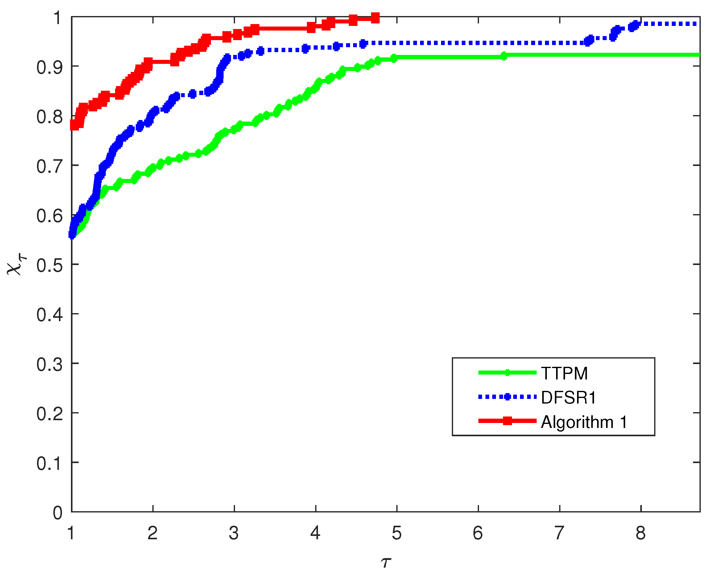
In order to conduct a comprehensive comparison across all algorithms, we make use of the performance profile framework developed by Dolan and Mor’e [32], which is standard in the field of numerical optimization for algorithmic performance assessment. Figure 1 illustrates the performance profiles for the number of iterations on a log 2 -scale, involving three algorithms: TTPM, DFSR1, and Algorithm 1.
In Figure 1, it can be observed that as τ increases, Algorithm 1 consistently achieves a higher proportion of solved problems than TTPM and DFSR1. Specifically, when τ reaches around 1.5, the curve of Algorithm 1 rises significantly faster and remains at the top afterward—this clearly demonstrates its notable advantage in iteration efficiency. In contrast, the proportion of solved problems for DFSR1 grows relatively slowly, while TTPM is less competitive in iteration performance compared to the other two algorithms.
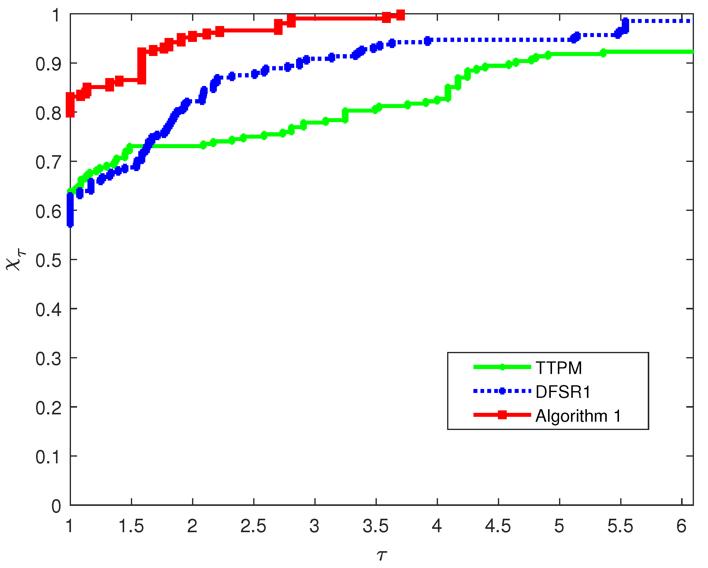
Figure 2 presents the performance regarding function evaluations. It is evident that Algorithm 1 solves the largest proportion of problems no matter what value τ takes. Consistent with the iteration results, Algorithm 1 performs exceptionally well, even when τ is small, the proportion of problems it solves already surpasses that of TTPM and DFSR1. Additionally, TTPM and DFSR1 show similar performance in function evaluations, but both are less efficient than Algorithm 1.
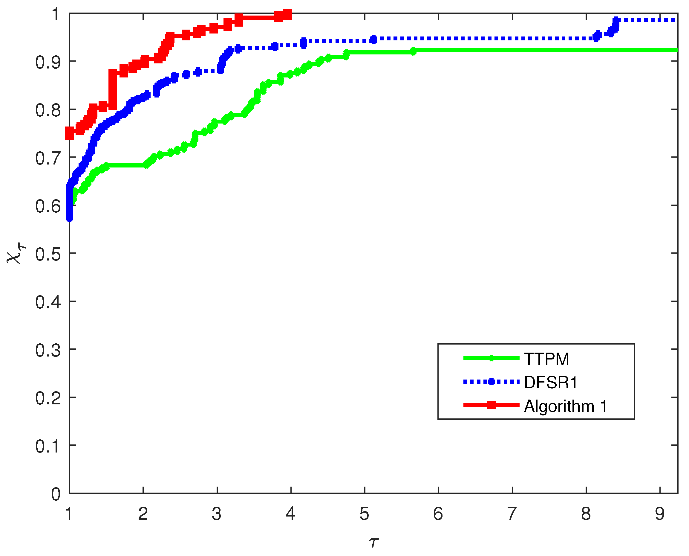
Figure 3 illustrates the performance differences in CPU time. As can be seen from the figure, the curve of Algorithm 1 takes the lead from the very beginning and stays at the highest level as τ increases. This means that within the entire range of τ values, Algorithm 1 outperforms DFSR1 and TTPM in CPU time efficiency. Whether it is the basic efficiency when τ is small or the ability to cover more problems when τ increases, Algorithm 1 can solve a higher proportion of test problems with shorter CPU time, fully demonstrating its stable advantage in computational speed.
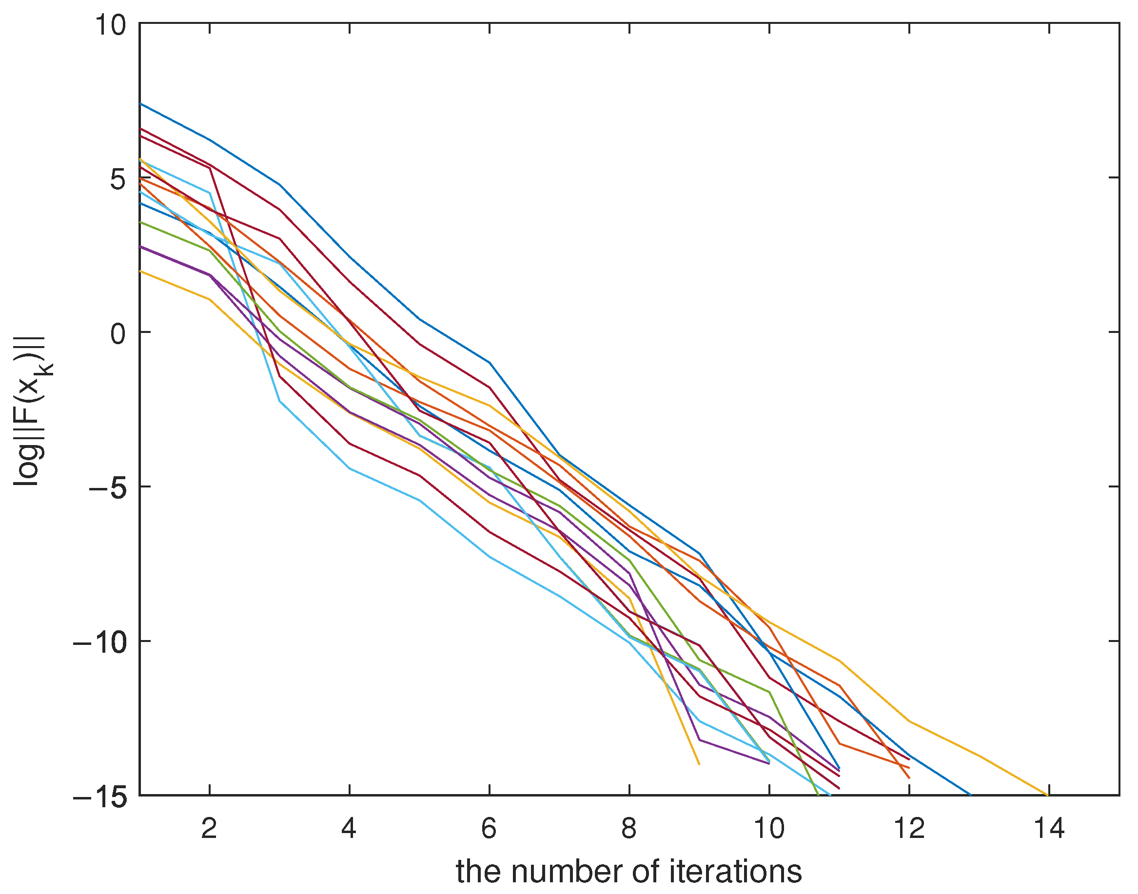
Moreover, we verify the convergence rate of Algorithm 1 through numerical experiments. Specifically, for Problem 8, we consider scenarios with two dimensions and eight initial points, resulting in 16 problem instances in total. We plot the curve of log F ( x k ) versus the number of iterations, as shown in Figure 4. It is evident that the curves of log F ( x k ) decrease linearly with the number of iterations, indicating that the Algorithm 1 exhibits linear convergence for Problem 8.
5. Results

In conclusion, this paper presents a new derivative-free method integrated with a symmetric rank-one update for solving constrained nonlinear systems of monotone equations. Rooted in the revised SR1 update formula and enhanced by projection techniques, the method exhibits distinct advantages: its search direction inherently satisfies sufficient descent and trust-region properties, eliminating reliance on line search techniques—a feature that simplifies practical implementation. Theoretical results confirm its global convergence under specified conditions, laying a solid foundation for its theoretical reliability. Comparative numerical experiments with two existing approaches further validate that the proposed method outperforms competitors in terms of iteration count, function evaluations, and CPU runtime, demonstrating superior reliability and robustness. These findings highlight the method’s potential as an efficient and stable tool for addressing constrained nonlinear monotone equations, with promising applications in related engineering and scientific computing fields.

Funding

This research was supported by the Zhejiang Provincial Natural Science Foundation of China under Grant No. LY23A010007 and the Huzhou Natural Science Foundation under Grant No. 2023YZ29.

Data Availability Statement

No new data were created or analyzed in this study.

Conflicts of Interest

The author declares no conflicts of interest.

References

  1. Prajna, S.; Parrilo, P.A.; Rantzer, A. Nonlinear control synthesis by convex optimization. IEEE Trans. Autom. Control 2004, 49, 310–314. [Google Scholar] [CrossRef]
  2. Ghaddar, B.; Marecek, J.; Mevissen, M. Optimal power flow as a polynomial optimization problem. IEEE Trans. Power Syst. 2016, 31, 539–546. [Google Scholar] [CrossRef]
  3. Hu, Y.P.; Wang, Y.J. An efficient projected gradient method for convex constrained monotone equations with applications in compressive sensing. J. Appl. Math. Phys. 2020, 8, 983–998. [Google Scholar] [CrossRef]
  4. Liu, J.K.; Du, L. A gradient projection method for the sparse signal reconstruction in compressive sensing. Appl. Anal. 2018, 97, 2122–2131. [Google Scholar] [CrossRef]
  5. Xiao, Y.H.; Wang, Q.Y.; Hu, Q.J. Non-smooth equations based method for l1-norm problems with applications to compressive sensing. Nonlinear Anal.—Theory Methods Appl. 2011, 74, 3570–3577. [Google Scholar] [CrossRef]
  6. Zhou, G.; Toh, K.C. Superlinear convergence of a Newton-type algorithm for monotone equations. J. Optim. Theory Appl. 2005, 125, 205–221. [Google Scholar] [CrossRef]
  7. Li, D.H.; Fukushima, M. A globally and superlinearly convergent Gauss-Newton based BFGS method for symmetric equations. SIAM J. Numer. Anal. 1999, 37, 152–172. [Google Scholar] [CrossRef]
  8. Yuan, G.L.; Wei, Z.X.; Lu, X.W. A BFGS trust-region method for nonlinear equations. Computing 2011, 92, 317–333. [Google Scholar] [CrossRef]
  9. Fang, X.W.; Ni, Q.; Zeng, M.L. A modified quasi-Newton method for nonlinear equations. J. Comput. Appl. Math. 2018, 328, 44–58. [Google Scholar] [CrossRef]
  10. Ibrahim, A.H.; Kumam, P.; Abubakar, A.B.; Abubakar, J. A method with inertial extrapolation step for convex constrained monotone equations. J. Inequal. Appl. 2021, 2021, 189. [Google Scholar] [CrossRef]
  11. Fang, X.W.; Ni, Q. A New Derivative-Free Conjugate Gradient Method for Large-Scale Nonlinear Systems of Equations. Bull. Aust. Math. Soc. 2017, 95, 500–511. [Google Scholar] [CrossRef]
  12. Kumam, P.; Abubakar, A.B.; Malik, M.; Ibrahim, A.H.; Pakkaranang, N.; Panyanak, B. A hybrid HS-LS conjugate gradient algorithm for unconstrained optimization with applications in motion control and image recovery. J. Comput. Appl. Math. 2023, 433, 115304. [Google Scholar] [CrossRef]
  13. Fang, X.W. A class of new derivative-free gradient type methods for large-scale nonlinear systems of monotone equations. J. Inequal. Appl. 2020, 2020, 93. [Google Scholar] [CrossRef]
  14. Solodov, M.V.; Svaiter, B.F. A globally convergent inexact Newton method for systems of monotone equations. In Reformulation: Nonsmooth, Piecewise Smooth, Semismooth and Smoothing Methods; Fukushima, M., Qi, L., Eds.; Springer: Berlin/Heidelberg, Germany, 1998; pp. 355–369. [Google Scholar]
  15. Li, Q.; Zheng, B. Scaled three-term derivative-free methods for solving large-scale nonlinear monotone equations. Numer. Algorithms 2021, 87, 1343–1367. [Google Scholar] [CrossRef]
  16. Dai, Z.; Zhu, H. A modified Hestenes-Stiefel-type derivative-free method for large-scale nonlinear monotone equations. Mathematics 2020, 8, 168. [Google Scholar] [CrossRef]
  17. Kimiaei, M.; Hassan Ibrahim, A.; Ghaderi, S. A subspace inertial method for derivative-free nonlinear monotone equations. Optimization 2025, 74, 269–296. [Google Scholar] [CrossRef]
  18. Liu, J.K.; Tang, B.; Zhang, N.; Xiong, J.; Gao, P.T.; Dong, X.L. A subspace derivative-free projection method for convex constrained nonlinear equations. Jpn. J. Ind. Appl. Math. 2025, 42, 197–221. [Google Scholar] [CrossRef]
  19. Kumam, P.; Abubakar, A.B.; Ibrahim, A.H.; Kura, H.U.; Panyanak, B.; Pakkaranang, N. Another hybrid approach for solving monotone operator equations and application to signal processing. Math. Methods Appl. Sci. 2022, 45, 7897–7922. [Google Scholar] [CrossRef]
  20. Xia, Y.; Li, D.; Wang, S. A modified two-term conjugate gradient-based projection algorithm for constrained nonlinear equations with applications. Bound. Value Probl. 2025, 2025, 89. [Google Scholar] [CrossRef]
  21. Fang, X.W. A derivative-free RMIL conjugate gradient method for constrained nonlinear systems of monotone equations. AIMS Math. 2025, 10, 11656–11675. [Google Scholar] [CrossRef]
  22. Zhang, N.; Liu, J.K.; Tang, B. A three-term projection method based on spectral secant equation for nonlinear monotone equations. Jpn. J. Ind. Appl. Math. 2024, 41, 617–635. [Google Scholar] [CrossRef]
  23. Abubakar, A.B.; Sabi’u, J.; Kumam, P.; Shah, A. Solving nonlinear monotone operator equations via modified SR1 update. J. Appl. Math. Comput. 2021, 67, 343–373. [Google Scholar] [CrossRef]
  24. Awwal, A.M.; Ishaku, A.; Halilu, A.S.; Stanimirović, P.S.; Pakkaranang, N.; Panyanak, B. Descent Derivative-Free Method Involving Symmetric Rank-One Update for Solving Convex Constrained Nonlinear Monotone Equations and Application to Image Recovery. Symmetry 2022, 14, 2375. [Google Scholar] [CrossRef]
  25. Rao, J.; Huang, N. A derivative-free scaling memoryless DFP method for solving large scale nonlinear monotone equations. J. Glob. Optim. 2023, 87, 641–677. [Google Scholar] [CrossRef]
  26. Tang, J.; Zhou, J. A two-step Broyden-like method for nonlinear equations. Numer. Algorithms 2025, 98, 1085–1105. [Google Scholar] [CrossRef]
  27. Ullah, N.; Sabi’u, J.; Shah, A. A derivative-free scaling memoryless Broyden–Fletcher–Goldfarb–Shanno method for solving a system of monotone nonlinear equations. Numer. Linear Algebra Appl. 2021, 28, e2374. [Google Scholar] [CrossRef]
  28. Broyden, C.G. A class of methods for solving nonlinear simultaneous equations. Math. Comput. 1965, 19, 577–593. [Google Scholar] [CrossRef]
  29. Barzilai, J.; Borwein, J.M. Two-point step size gradient methods. IMA J. Numer. Anal. 1988, 8, 141–148. [Google Scholar] [CrossRef]
  30. Gao, G.P.; Tao, W.; Li, X.L.; Wu, Y.F. An efficient three-term conjugate gradient-based algorithm involving spectral quotient for solving convex constrained monotone nonlinear equations with applications. Comput. Appl. Math. 2022, 41, 89. [Google Scholar]
  31. Sabi’u, J.; Sirisubtawee, S. An inertial Dai-Liao conjugate method for convex constrained monotone equations that avoids the direction of maximum magnification. J. Appl. Math. Comput. 2024, 70, 4319–4351. [Google Scholar] [CrossRef]
  32. Dolan, E.; Mor’e, J. Benchmarking optimization software with performance profiles. Math. Program. 2001, 91, 201–213. [Google Scholar] [CrossRef]
Figure 1. Performance profiles for the number of iterations on a log 2 scale.
Symmetry 17 01956 g001
Figure 2. Performance profiles for the number of function evaluations on a log 2 scale.
Symmetry 17 01956 g002
Figure 3. Performance profiles for the CPU time on a log 2 scale.
Symmetry 17 01956 g003
Figure 4. Convergence rate analysis: log F ( x k ) vs. the number of iterations for Problem 8.
Symmetry 17 01956 g004
Table 1. The results of three algorithms for Problems 1–5.
ProbDimSta TTPM DFSR1 Alg.1
NiterNfunTcpu F * NiterNfunTcpu F * Niter Nfun Tcpu F *
P110,000 x 1 18530.0135 4.36 × 10 7 19390.0118 8.97 × 10 7 10280.0063 2.25 × 10 7
x 2 18540.0093 4.36 × 10 7 18390.0100 7.75 × 10 7 9260.0045 2.34 × 10 7
x 3 17520.0092 4.36 × 10 7 18380.0064 6.69 × 10 7 9260.0045 2.21 × 10 7
x 4 17490.0073 5.00 × 10 7 18370.0072 7.72 × 10 7 8280.0045 3.09 × 10 7
x 5 14420.0064 5.74 × 10 7 18380.0073 6.60 × 10 7 9330.0056 7.41 × 10 7
x 6 16480.0076 5.89 × 10 7 19400.0082 9.70 × 10 7 8230.0042 4.59 × 10 7
x 7 20550.0083 7.53 × 10 7 15320.0061 9.41 × 10 7 13520.0089 1.72 × 10 7
x 8 20550.0089 7.99 × 10 7 15320.0056 9.40 × 10 7 13520.0088 1.72 × 10 7
50,000 x 1 18530.0316 9.76 × 10 7 24570.0394 5.12 × 10 7 10280.0220 5.04 × 10 7
x 2 18540.0291 9.76 × 10 7 19410.0302 6.91 × 10 7 9260.0154 5.24 × 10 7
x 3 17520.0328 9.76 × 10 7 19400.0240 5.97 × 10 7 9260.0165 4.94 × 10 7
x 4 17490.0318 8.26 × 10 7 21440.0376 6.12 × 10 7 8280.0167 6.92 × 10 7
x 5 14420.0231 9.48 × 10 7 19410.0258 6.78 × 10 7 10370.0227 2.69 × 10 7
x 6 16480.0309 9.73 × 10 7 18390.0239 4.71 × 10 7 9260.0159 1.23 × 10 7
x 7 21580.0356 5.74 × 10 7 16330.0257 1.12 × 10 8 13520.0327 3.85 × 10 7
x 8 21580.0356 5.81 × 10 7 16330.0207 1.12 × 10 8 13520.0353 3.85 × 10 7
P210,000 x 1 1150.00210 1120.00130 1120.00150
x 2 120.00040 120.00040 120.00040
x 3 120.00040 240.00060 120.00030
x 4 130.00040 260.00090 130.00050
x 5 15310.0060 8.06 × 10 7 130.00040 390.00180
x 6 15300.0040 5.08 × 10 7 240.00050 4120.00160
x 7 19390.0069 4.93 × 10 7 250.00060 13490.0059 7.07 × 10 7
x 8 19390.0073 4.93 × 10 7 250.00050 13490.0053 7.06 × 10 7
50,000 x 1 1150.00940 1120.00780 1120.00670
x 2 120.00130 140.00240 120.00130
x 3 120.00130 130.00260 120.00180
x 4 130.00160 260.00420 130.00230
x 5 16330.0250 8.11 × 10 7 130.00140 390.00600
x 6 15300.0220 8.57 × 10 7 240.00220 4120.00620
x 7 19390.0268 8.34 × 10 7 260.00430 14530.0280 5.41 × 10 7
x 8 19390.0210 8.33 × 10 7 260.00280 14530.0245 5.40 × 10 7
P310,000 x 1 260.00180 7300.00670 5200.00400
x 2 140.00100 170.00190 140.00100
x 3 130.00040 360.00090 130.00040
x 4 17350.0056 9.73 × 10 7 130.00040 390.00160
x 5 15310.0050 9.35 × 10 7 360.00070 390.00100
x 6 130.00040 130.00030 130.00040
x 7 17350.0055 7.25 × 10 7 130.00050 390.00160
x 8 17350.0049 7.25 × 10 7 130.00030 390.00110
50,000 x 1 260.00690 10530.04640 5200.01510
x 2 140.0040 180.00940 140.00410
x 3 130.0020 360.00390 130.00210
x 4 18370.024 7.40 × 10 7 130.00210 390.00600
x 5 16330.019 9.40 × 10 7 360.00400 390.00520
x 6 130.0010 130.00110 130.00140
x 7 18370.020 5.51 × 10 7 130.00160 390.00380
x 8 18370.019 5.51 × 10 7 130.00130 390.00430
P410,000 x 1 651290.045 5.57 × 10 7 371070.0320 5.92 × 10 7 391940.0513 3.57 × 10 7
x 2 621230.039 8.00 × 10 7 24500.0159 7.53 × 10 7 402030.0580 3.13 × 10 7
x 3 581150.037 9.80 × 10 7 25510.0160 1.66 × 10 7 533040.0777 5.93 × 10 7
x 4 631250.039 9.92 × 10 7 23460.0149 6.82 × 10 7 432230.0576 3.90 × 10 7
x 5 561120.043 6.24 × 10 7 28590.0191 5.96 × 10 7 442220.0589 4.09 × 10 7
x 6 591190.044 6.39 × 10 7 24480.0149 4.37 × 10 7 482360.0673 6.37 × 10 7
x 7 641300.042 7.85 × 10 7 25520.0166 4.37 × 10 7 482610.0736 4.73 × 10 7
x 8 531060.037 8.30 × 10 7 25520.0192 9.19 × 10 7 663440.0948 6.78 × 10 7
50,000 x 1 581140.165 8.06 × 10 7 1489721.1514 9.24 × 10 7 422170.2666 3.18 × 10 7
x 2 571120.163 6.96 × 10 7 1489721.1459 7.82 × 10 7 432180.2650 4.99 × 10 7
x 3 601180.167 8.95 × 10 7 1499741.1507 3.91 × 10 7 331530.1984 8.18 × 10 7
x 4 551080.153 8.74 × 10 7 1499741.1705 5.57 × 10 7 512560.3231 9.14 × 10 7
x 5 591170.166 9.32 × 10 7 1499741.1812 3.60 × 10 7 351630.2110 4.80 × 10 7
x 6 591160.166 7.86 × 10 7 1499741.1622 3.83 × 10 7 492580.3151 4.09 × 10 7
x 7 591160.165 8.32 × 10 7 1499741.1511 7.77 × 10 7 422070.2585 9.92 × 10 7
x 8 601180.167 6.59 × 10 7 1499741.1449 3.51 × 10 7 412120.2644 9.79 × 10 7
P510,000 x 1 27820.009 9.86 × 10 7 20720.0069 6.04 × 10 7 15720.0070 7.38 × 10 7
x 2 28850.010 7.36 × 10 7 180.00060 140.00040
x 3 24730.008 7.51 × 10 7 150.00040 140.00040
x 4 23700.008 7.36 × 10 7 11270.0031 8.82 × 10 7 14670.0064 4.67 × 10 7
x 5 19580.006 5.80 × 10 7 140.00040 12570.0055 8.98 × 10 7
x 6 19580.006 7.82 × 10 7 270.00070 140.00040
x 7 21640.007 7.05 × 10 7 390.0009 9.02 × 10 11 13620.0057 6.82 × 10 7
x 8 23700.008 6.17 × 10 7 280.00060 13620.0059 6.81 × 10 7
50,000 x 1 25760.026 7.05 × 10 7 291380.0460 5.20 × 10 7 16770.0232 5.73 × 10 7
x 2 30910.030 4.36 × 10 7 190.00240 140.00100
x 3 25760.027 6.75 × 10 7 160.00180 140.00140
x 4 21640.023 7.84 × 10 7 13350.0121 4.92 × 10 7 14670.0215 7.24 × 10 7
x 5 17520.017 9.14 × 10 7 140.00120 13620.0207 4.40 × 10 7
x 6 19580.019 8.08 × 10 7 270.00190 140.00100
x 7 26790.028 8.18 × 10 7 11280.0106 8.06 × 10 7 14670.0215 6.02 × 10 7
x 8 20610.020 9.45 × 10 7 3130.0041 1.80 × 10 7 14670.0214 6.02 × 10 7
Table 2. The results of three algorithms for Problems 6–10.
ProbDimSta TTPM DFSR1 Alg.1
Niter Nfun Tcpu F * Niter Nfun Tcpu F * Niter Nfun Tcpu F *
P610,000 x 1 120.0020 120.00130 120.00120
x 2 120.0010 120.00090 120.00080
x 3 120.0020 120.00220 120.00220
x 4 230.0020 9310140.32960 230.00180
x 5 340.0040 10411230.33770 340.00220
x 6 120.0010 120.00050 120.00050
x 7 230.0030 909770.26250 230.00120
x 8 230.0030 899660.24650 230.00140
50,000 x 1 120.0050 120.00380 120.00360
x 2 120.0040 130.00600 120.00410
x 3 120.0060 120.00630 120.00600
x 4 230.0060 9310141.33880 230.00550
x 5 340.0140 10611461.47210 340.00820
x 6 120.0020 120.00190 120.00220
x 7 230.0110 9310121.14410 230.00540
x 8 230.0120 9310121.11580 230.00530
P710,000 x 1 670.0050 11550.02060 340.00210
x 2 120.0010 140.00130 120.00080
x 3 120.0010 120.00060 120.00060
x 4 230.0010 120.00060 230.00120
x 5 120.0010 120.00070 120.00070
x 6 120.0010 120.00070 120.00070
x 7 nannannan 1.81 × 10 3 340.00160 340.00190
x 8 nannannan 2.50 × 10 3 340.00160 340.00200
50,000 x 1 670.0190 221390.23290 340.00970
x 2 120.0040 150.00770 120.00330
x 3 120.0020 130.00440 120.00250
x 4 230.0060 240.00640 230.00500
x 5 120.0040 120.00320 120.00320
x 6 120.0030 120.00310 120.00310
x 7 nannannan 2.18 × 10 2 340.00670 450.0096 5.41 × 10 29
x 8 nannannan 2.32 × 10 2 340.00660 340.00830
P810,000 x 1 14560.011 4.84 × 10 7 471870.0413 9.36 × 10 7 11530.0079 2.53 × 10 7
x 2 14560.008 5.97 × 10 7 431570.0329 9.25 × 10 7 12580.0105 9.70 × 10 7
x 3 12490.007 9.68 × 10 7 30940.0138 8.40 × 10 7 11530.0085 7.28 × 10 7
x 4 12480.009 6.37 × 10 7 371180.0246 7.81 × 10 7 12550.0098 5.31 × 10 7
x 5 13530.009 7.80 × 10 7 341060.0190 6.89 × 10 7 9430.0066 8.20 × 10 7
x 6 13530.008 4.47 × 10 7 321000.0157 8.33 × 10 7 11530.0081 6.68 × 10 7
x 7 281120.016 9.00 × 10 7 461270.0214 9.56 × 10 7 10470.0077 9.19 × 10 7
x 8 281120.017 9.01 × 10 7 461270.0262 9.75 × 10 7 10470.0077 8.84 × 10 7
50,000 x 1 14560.044 6.53 × 10 7 663550.3356 7.73 × 10 7 11530.0397 5.66 × 10 7
x 2 14560.040 8.05 × 10 7 451750.1563 8.48 × 10 7 13630.0408 2.57 × 10 7
x 3 13530.029 4.37 × 10 7 351110.0661 8.93 × 10 7 12580.0329 7.43 × 10 7
x 4 13520.037 4.77 × 10 7 401350.0962 6.45 × 10 7 14650.0446 2.97 × 10 7
x 5 14570.035 3.52 × 10 7 361160.0720 8.18 × 10 7 10480.0278 8.45 × 10 7
x 6 13530.031 9.99 × 10 7 361140.0771 9.29 × 10 7 11530.0342 7.24 × 10 8
x 7 301200.082 5.15 × 10 7 421210.0846 5.79 × 10 7 11520.0299 3.82 × 10 7
x 8 301200.072 5.15 × 10 7 421210.0930 6.08 × 10 7 11520.0354 3.79 × 10 7
P910,000 x 1 8410.044 4.86 × 10 7 36830.0955 7.04 × 10 7 13600.0404 4.88 × 10 7
x 2 8200.010 4.86 × 10 7 36760.0720 7.04 × 10 7 16810.0235 7.84 × 10 7
x 3 5200.006 2.06 × 10 7 10450.0153 1.65 × 10 7 16920.0220 8.46 × 10 7
x 4 5220.006 6.38 × 10 8 7300.0077 8.14 × 10 7 11540.0125 1.00 × 10 7
x 5 4170.004 1.83 × 10 8 7290.0063 6.43 × 10 7 14810.0156 6.80 × 10 7
x 6 4170.003 2.30 × 10 8 7290.0068 4.38 × 10 7 14810.0172 8.01 × 10 7
x 7 341520.036 7.70 × 10 7 531620.0386 9.71 × 10 7 17970.0211 4.42 × 10 7
x 8 351460.034 7.14 × 10 7 531620.0389 9.73 × 10 7 17970.0199 4.27 × 10 7
50,000 x 1 9450.192 1.83 × 10 7 38870.4673 7.43 × 10 7 15700.1919 9.10 × 10 7
x 2 9240.043 1.83 × 10 7 38800.3674 7.43 × 10 7 17870.1117 4.93 × 10 7
x 3 5200.023 4.60 × 10 7 171070.1340 4.13 × 10 7 17980.0888 7.71 × 10 7
x 4 5220.027 1.43 × 10 7 8340.0359 8.64 × 10 7 11540.0525 2.24 × 10 7
x 5 4170.015 4.10 × 10 8 8340.0306 8.56 × 10 7 15870.0787 4.05 × 10 7
x 6 4170.016 5.15 × 10 8 8340.0294 9.31 × 10 7 15870.0825 7.08 × 10 7
x 7 381670.148 5.33 × 10 7 541690.1662 8.32 × 10 7 17970.0865 9.81 × 10 7
x 8 371640.150 4.46 × 10 7 541690.1639 8.32 × 10 7 17970.0877 9.74 × 10 7
P1010,000 x 1 444360.071 4.55 × 10 7 1762700.082 9.81 × 10 7 201030.018 8.13 × 10 7
x 2 26440.011 6.36 × 10 7 58670.020 9.73 × 10 7 23970.019 6.60 × 10 7
x 3 30490.012 4.76 × 10 7 1611670.056 9.89 × 10 7 16650.012 6.48 × 10 7
x 4 20410.012 7.36 × 10 7 1221300.046 9.76 × 10 7 16660.015 6.91 × 10 7
x 5 30480.013 8.22 × 10 7 68740.023 9.86 × 10 7 16610.015 5.23 × 10 7
x 6 26440.010 8.51 × 10 7 1081140.037 9.81 × 10 7 19770.016 6.43 × 10 7
x 7 32540.016 5.52 × 10 7 2152240.073 9.93 × 10 7 21990.019 4.38 × 10 7
x 8 23460.013 9.70 × 10 7 961010.036 9.76 × 10 7 14520.011 7.02 × 10 7
50,000 x 1 524600.347 4.79 × 10 7 2233650.396 9.76 × 10 7 201040.081 9.68 × 10 7
x 2 28510.050 9.68 × 10 7 2082430.322 9.75 × 10 7 18720.056 9.44 × 10 7
x 3 29480.052 4.81 × 10 7 2232570.349 9.90 × 10 7 18760.070 3.51 × 10 7
x 4 28500.051 9.91 × 10 7 1671810.232 9.99 × 10 7 16660.065 9.02 × 10 7
x 5 28470.053 7.66 × 10 7 971080.148 9.94 × 10 7 16610.057 6.45 × 10 7
x 6 25500.046 9.95 × 10 7 2122310.320 9.80 × 10 7 14500.045 3.10 × 10 7
x 7 40620.068 9.36 × 10 7 1761860.259 9.86 × 10 7 241430.109 8.85 × 10 7
x 8 24500.052 5.40 × 10 7 62680.086 9.76 × 10 7 16600.055 5.72 × 10 7
Table 3. The results of three algorithms for Problems 11–13.
ProbDimSta TTPM DFSR1 Alg.1
Niter Nfun Tcpu F * Niter Nfun Tcpu F * Niter Nfun Tcpu F *
P1110,000 x 1 201340.031 9.11 × 10 7 1120.0040 1120.0040
x 2 150.0020 1120.0050 2100.0040
x 3 160.0020 1120.0030 160.0010
x 4 171030.022 6.13 × 10 7 6400.0100 4250.0060
x 5 171030.021 8.70 × 10 7 2120.0020 3170.0030
x 6 171020.018 6.39 × 10 7 170.0010 160.0010
x 7 30419040.3890 nannannan 7.17 × 10 + 2 272090.0280
x 8 49236360.8920 nannannan 9.54 × 10 + 2 12720.0110
50,000 x 1 211400.133 6.84 × 10 7 1120.0200 1120.0200
x 2 150.0090 1120.0210 2100.0160
x 3 160.0080 1120.0120 160.0070
x 4 181090.099 4.60 × 10 7 10720.0850 4250.0290
x 5 181090.083 8.68 × 10 7 3180.0180 3170.0130
x 6 181080.079 4.79 × 10 7 180.0070 160.0050
x 7 28416401.4640 nannannan 9.89 × 10 + 2 211560.0890
x 8 30017141.6370 11640.060 8.10 × 10 7 241750.0970
P1210,000 x 1 nannannan 6.87 × 10 5 120.0010 360.0080
x 2 120.0030 170.0080 120.0020
x 3 120.0020 120.0020 120.0010
x 4 nannannan 6.84 × 10 5 120.0000 350.0060
x 5 nannannan 6.76 × 10 5 340.0080 340.0070
x 6 120.0020 120.0020 120.0020
x 7 nannannan 4.50 × 10 5 22230.018 9.61 × 10 7 19200.020 5.51 × 10 7
x 8 nannannan 4.50 × 10 5 22230.018 9.61 × 10 7 19210.023 9.26 × 10 7
50,000 x 1 nannannan 1.54 × 10 4 120.0060 360.0340
x 2 120.0120 180.0430 120.0110
x 3 120.0070 140.0170 120.0070
x 4 nannannan 1.53 × 10 4 120.0010 350.0290
x 5 nannannan 1.51 × 10 4 340.0330 340.0330
x 6 120.0120 120.0110 120.0110
x 7 nannannan 1.01 × 10 4 39410.386 9.86 × 10 7 22230.099 2.03 × 10 7
x 8 nannannan 1.01 × 10 4 39410.386 9.86 × 10 7 21230.097 5.66 × 10 7
P1310,000 x 1 51580.0130 7680.0090 6270.0030
x 2 51590.0130 7680.0090 6270.0030
x 3 73240.0250 1120.0020 4150.0020
x 4 450.0010 9900.0180 4150.0020
x 5 nannannan 1.56 × 10 + 1 10710.0100 9400.0060
x 6 120.0000 120.0000 120.0000
x 7 450.0010 9900.0140 4150.0020
x 8 72540.0200 151560.0240 5160.0030
50,000 x 1 51760.0480 6570.0210 6270.0120
x 2 51740.0510 6570.0190 6270.0100
x 3 nannannan 3.53 × 10 + 1 7680.0290 4150.0200
x 4 51640.0510 7680.0490 4150.0210
x 5 6590.0200 8690.0420 7280.0140
x 6 120.0010 120.0010 120.0010
x 7 51610.0480 7680.0410 4150.0160
x 8 73110.0940 9900.0550 4150.0070
Table 4. Sensitivity analysis of parameter γ for Algorithm 1.
γ = 1 γ = 1.2 γ = 1.4
Niter ¯ Nfun ¯ Tcpu ¯ F * ¯ Niter ¯ Nfun ¯ Tcpu ¯ F * ¯ Niter ¯ Nfun ¯ Tcpu ¯ F * ¯
14.45772.1880.044 3.088 × 10 7 10.52948.1830.030 2.710 × 10 7 10.56549.9090.033 2.872 × 10 7
Table 5. Sensitivity analysis of parameter ρ for Algorithm 1.
ρ = 0.4 ρ = 0.5 ρ = 0.6
Niter ¯ Nfun ¯ Tcpu ¯ F * ¯ Niter ¯ Nfun ¯ Tcpu ¯ F * ¯ Niter ¯ Nfun ¯ Tcpu ¯ F * ¯
15.08765.5190.038 3.574 × 10 7 10.52948.1830.030 2.710 × 10 7 10.85652.3750.035 2.790 × 10 7
Table 6. Sensitivity analysis of parameter c for Algorithm 1.
c = 0.05 c = 0.1 c = 0.2
Niter ¯ Nfun ¯ Tcpu ¯ F * ¯ Niter ¯ Nfun ¯ Tcpu ¯ F * ¯ Niter ¯ Nfun ¯ Tcpu ¯ F * ¯
10.59048.9130.031 2.708 × 10 7 10.52948.1830.030 2.710 × 10 7 10.86152.3850.035 2.478 × 10 7
Table 7. Sensitivity analysis of parameter ζ 1 and ζ 2 for Algorithm 1.
ζ 1 = 0.01 ζ 2 = 0.8 ζ 1 = 0.001 ζ 2 = 0.8 ζ 1 = 0.001 ζ 2 = 8
Niter ¯ Nfun ¯ Tcpu ¯ F * ¯ Niter ¯ Nfun ¯ Tcpu ¯ F * ¯ Niter ¯ Nfun ¯ Tcpu ¯ F * ¯
10.52948.1830.031 2.710 × 10 7 10.52948.1830.030 2.710 × 10 7 10.53249.0430.031 2.699 × 10 7
Disclaimer/Publisher’s Note: The statements, opinions and data contained in all publications are solely those of the individual author(s) and contributor(s) and not of MDPI and/or the editor(s). MDPI and/or the editor(s) disclaim responsibility for any injury to people or property resulting from any ideas, methods, instructions or products referred to in the content.