Abstract
This extensive study introduces the Rosenbrock method (RosM) for numerically integrating the chaotic Lorenz system, with a focus on its ability to preserve the system’s intrinsic dynamical and structural symmetries. The Lorenz system exhibits significant symmetry, most notably an inversion symmetry , which is a fundamental feature of its chaotic attractor. We lay forth the algorithm and, after systematic comparisons to explicit Runge–Kutta higher-order schemes and semi-analytically obtained solutions, show that the second-order Rosenbrock method performs with excellent accuracy and stability. Crucially, we demonstrate that RosM reliably preserves the system’s symmetry over long-term integration, a property where some explicit methods can exhibit subtle drift. We give a formal error characterization, assess the computational efficiency, and verify the method via bifurcation analysis to support that RosM is a robust and symmetry-aware tool for simulating chaotic systems.
Keywords:
chaotic Lorenz system; Rosenbrock method; symmetry preservation; seventh-eighth-order Runge-Kutta method (RK78) MSC:
65L05; 65P20; 37M05; 65L20
1. Introduction
The analysis of nonlinear systems of ODEs presents a fundamental challenge in applied mathematics and physics, primarily due to the general unavailability of exact closed-form analytical solutions. To overcome this difficulty, various numerical and semi-analytical approaches have been developed. Among them, the Adomian Decomposition Method (ADM) [1,2,3] has emerged as a powerful and elegant tool. Unlike traditional numerical techniques that rely on discretization and linearization, the ADM provides an analytical solution in the form of a rapidly convergent infinite power series with systematically computable terms [4,5].This capability to handle nonlinear problems without perturbation has made the method popular for studying a wide range of phenomena, as evidenced by its applications to prey–predator systems [6], delay equations [7], and partial differential equations [8,9]. In [10], the ResM was used to solve the differential Sylvester matrix equations, and it was later developed for fractional differential matrix equations in [11]. The numerical integration of chaotic systems represents a particularly challenging domain where traditional methods often face limitations due to sensitivity to initial conditions and long-term stability requirements. While explicit Runge–Kutta methods have dominated this field, their stability constraints and adaptive step-size requirements can limit their efficiency for certain classes of problems.
The Lorenz system [12,13], a paradigm of deterministic chaos, constitutes a demanding test bed for any numerical method due to its extreme sensitivity to initial conditions. Its intrinsic chaotic behavior makes it an ideal candidate for assessing the accuracy and stability of integration algorithms. The application of ADM to the Lorenz system has been studied in the past, notably by Guellal et al. [14], and more recently by Hashim et al. [5]. These works, among others [15,16,17,18,19], have often compared the performance of ADM against other methods, such as the 4-order Runge–Kutta method [19] or the Runge–Kutta–Verner method [15,16]. The majority of these studies have focused on the effect of the time step size () on the solution’s accuracy. However, these previous studies have largely overlooked the potential of implicit methods like the Rosenbrock scheme for chaotic system integration. Rosenbrock methods, being linearly implicit, offer a compelling compromise between the stability of fully implicit methods and the computational efficiency of explicit approaches.
However, for modern adaptive numerical methods like the RK78, the critical parameter governing accuracy and efficiency is not a fixed step size, but a prescribed error tolerance. A comprehensive and fair comparison between a semi-analytical method like ADM and an advanced numerical method like RK78 must therefore necessarily account for this fundamental parameter. In this work, we propose an in-depth comparative study that addresses this gap. Our primary contributions include:
- A comprehensive evaluation of the second-order RosM for both non-chaotic and chaotic regimes of the Lorenz system.
- Detailed comparison with RK78 and ode45 and semi-analytical approaches ADM and MHPM.
- Systematic analysis of error propagation.
- Validation through bifurcation analysis demonstrating RosM’s capability for qualitative dynamical analysis.
- Practical guidelines for step size selection and method application.
We evaluate the accuracy of the ADM by comparing it against benchmark results generated by the RK78 method (using, for instance, the Dormand–Prince algorithm) for a range of error tolerances. Following the approach of Hashim et al. [5], we use a fixed time step of for ADM. Our primary objective is to quantify the combined impact of time step and error tolerance on the accuracy of ADM to solve the chaotic Lorenz system. Furthermore, we extend this comparative analysis to include the Rosenbrock method [20], an implicit scheme known for its stability when solving so-called “stiff” systems. This inclusion broadens the perspective and allows for a comparison of the relative performances of a semi-analytical method (ADM), an adaptive explicit method (RK78), and an implicit method (Rosenbrock) on this famous problem.
We consider the Lorenz system in [21]:
where the parameters are set to their classic values: , , and , ensuring chaotic behavior.
The Lorenz system (1) is not only a benchmark for chaotic behavior but also a canonical example of a dynamical system with inherent symmetry. It is equivariant under the transformation , meaning that if is a solution, then so is . This symmetry is a fundamental characteristic of the Lorenz attractor, manifesting in its two ‘wings’. A reliable numerical method must preserve this structural property over long integration times to accurately reflect the true dynamics. While explicit methods like RK78 are highly accurate, their adaptive step-size control and local truncation errors can sometimes lead to a subtle breaking of this symmetry over very long simulations. Implicit methods like the Rosenbrock scheme, with their superior stability, offer a promising alternative for symmetry preservation.
The significance of symmetry-preserving integration methods extends far beyond the Lorenz system, finding crucial applications across diverse scientific domains where structural invariants must be rigorously maintained. In fluid dynamics, preserving Galilean and rotational symmetries ensures physically consistent turbulence simulations and prevents numerical artifacts in large-eddy simulations. For plasma physics, symmetry-aware methods maintain essential conservation laws in magnetohydrodynamic simulations, particularly in tokamak confinement studies where broken symmetries can lead to unphysical plasma behavior. In climate modeling, long-term integration of atmospheric circulation models demands symmetry preservation to avoid biased predictions that may arise from accumulated numerical drift. The Rosenbrock approach demonstrated in this work provides a robust framework for such applications, offering both computational efficiency and reliable symmetry maintenance.
1.1. Novelty and Contribution
While the RosM is well known for stiff systems, its application to the chaotic Lorenz system with a systematic comparison against high-order adaptive methods (like RK78) and semi-analytical methods (like ADM and MHPM) under error tolerance control is underexplored. Our work bridges this gap by providing:
- Comprehensive methodology: Detailed implementation of the two-stage Rosenbrock method specifically tailored for the Lorenz system, including Jacobian computation and linear system solution strategies.
- Extended analysis: Simulation times extended to to properly capture long-term chaotic behavior and transient dynamics, addressing a key limitation in previous studies.
- Multi-faceted validation: Combination of quantitative error analysis, phase portrait examination, and bifurcation diagram generation to thoroughly validate method performance.
- Practical guidelines: Systematic approach to step size selection balancing accuracy, stability, and computational efficiency.
1.2. Advantages and Limitations
- Advantages of RosM:
- –
- Implicit nature ensures better stability for stiff or mildly stiff problems.
- –
- Competitive accuracy even with a fixed step size, without requiring adaptive step-size control.
- –
- Efficient for long-term integration where explicit methods may become unstable.
- –
- Predictable computational cost per time step.
- Limitations:
- –
- Requires solving a linear system at each step, which can be computationally expensive.
- –
- Requires Jacobian computation, which may be complex for some systems.
- –
- Less common in non-stiff chaotic systems compared to explicit Runge–Kutta methods.
2. Rosenbrock Method: Theoretical Foundation and Implementation
2.1. Theoretical Background
The RosM belong to the class of linearly implicit Runge–Kutta methods, first introduced by H. H. Rosenbrock in 1963 [20]. These methods represent a compromise between fully implicit and explicit methods, offering improved stability properties while maintaining reasonable computational efficiency.
For the general autonomous initial value problem:
a v-stage RosM is defined by the following computational scheme:
where the stage vectors are obtained by solving the linear systems:
Here, h is the step size, is the Jacobian matrix evaluated at , and the coefficients , , determine the method’s order and stability properties. The coefficients and are chosen as
which simplifies the derivation of the order conditions. We suppose throughout the paper that for all i.
2.2. Second-Order, Two-Stage RosM
For our implementation, we employ a second-order, two-stage RosM () with the following coefficient matrix:
The specific coefficients used in our implementation are:
This choice of coefficients ensures the method is L-stable, a desirable property for stiff systems.
2.3. Application to the Lorenz System
For the Lorenz system defined in Equation (1), we define the state vector and the right-hand side function:
The Jacobian matrix of the Lorenz system is:
For , we have
and
We obtain the two following system matrix equations:
and
2.4. Computational Algorithm
The complete Algorithm 1 for the two-stage RosM applied to the Lorenz system is as follows:
| Algorithm 1 Two-stage RosM for Lorenz system |
| Require: Initial conditions , final time , parameters , R, , step size h Ensure: Numerical solution for
|
2.5. Stability Analysis
For a v-stage RosM, the stability function is given by:
where and are polynomials determined by the method’s coefficients. For our specific method with , the coefficients (6). The stability function for a two-stage RosM is:
Consider the scalar test equation:
With the two-stage RosM:
- Stage 1:
- for all ,
- .
Condition 2:
Since , we have:
Condition 1: For , we must show that . Consider with . We require:
This is equivalent to:
For , we have . The stability condition is satisfied because the method is specifically designed with this to be L-stable.
The second-order Rosenbrock method with is L-stable because:
- ,
- for all ,
- The stability function decays rapidly for large values.
This property ensures excellent stability for stiff systems and allows the use of larger time steps compared to explicit methods.
2.6. Computational Complexity
Each time step of the algorithm requires:
- 1 Jacobian evaluation: operations (analytical form available)
- 2 Function evaluations: operations each
- 2 Linear system solutions: For a system, this requires operations using direct methods
- Vector operations: operations
The overall computational cost per time step is therefore constant, and the total cost scales as where N is the number of time steps.
2.7. Error Analysis
The local truncation error (LTE) and global error analysis for the second-order Rosenbrock method can be rigorously derived through Taylor series expansion and stability analysis.
2.7.1. Local Truncation Error (LTE)
For the second-order Rosenbrock method, the local truncation error represents the error committed in a single time step when the previous solution is exact. Through Taylor series expansion of both the exact solution and numerical approximation, we obtain. The exact solution development:
The numerical approximation for our second-order method matches the Taylor expansion up to second order:
The local truncation error is therefore:
2.7.2. Global Error
For a consistent and stable method, the global error accumulates local errors over time steps. Using stability analysis. Let be the global error at time . The error propagation satisfies:
where L is the Lipschitz constant of . Iterating this inequality yields:
Since and assuming exact initial conditions (), we obtain:
2.7.3. Numerical Verification
Our experimental results in Section 3 confirm this second-order convergence:
- For : global error to .
- For : global error to .
The error reduction ratio:
perfectly matches the expected second-order convergence.
2.7.4. Theoretical Foundation
The order conditions for Rosenbrock methods ensure that the coefficients are chosen to cancel lower-order error terms. For a second-order method, the conditions are:
Our specific coefficients satisfy these conditions, guaranteeing second-order accuracy. This error analysis establishes the theoretical foundation for the convergence behavior observed in our numerical experiments and validates the second-order accuracy of the implemented Rosenbrock method.
2.8. Implementation Details
Our MATLAB implementation includes the following key features:
- Matrix assembly: The linear system matrix is assembled explicitly at each time step.
- Linear solver: We employ MATLAB’s built-in LU decomposition with partial pivoting (\operator) for robust solution of the linear systems.
- Jacobian computation: The Jacobian is computed analytically using Equation (8), ensuring accuracy and efficiency.
- Memory management: Solutions are stored efficiently, with optional down-sampling for very long simulations.
2.9. Advantages for Chaotic Systems
The RosM offers several advantages for simulating chaotic systems like the Lorenz system:
- Improved stability: The L-stability property prevents numerical instability that can occur with explicit methods in stiff regions of phase space.
- Consistent accuracy: Maintains second-order accuracy throughout the simulation, unlike some explicit methods that may suffer from order reduction.
- Reliable long-term integration: The implicit nature provides more reliable long-term behavior prediction, crucial for chaotic system analysis.
- Fixed step size: Allows for predictable computational costs and simplifies error analysis compared to adaptive methods.
3. Results and Discussion
In this section, we show the application of the RosM to solve Lorenz system. We compare our method (Algorithm 1) presented in this paper, ADM [22], and MHPM [23]. All the experiments were performed on a laptop with an Intel Core i3 processor and 4 GB of RAM, using MATLAB 2020b. Let
3.1. Non-Chaotic Solutions
First, we consider the non-chaotic case with the other parameters as given above. The results in Table 1 demonstrate RosM’s excellent performance in the non-chaotic regime. The method achieves errors on the order of to with , improving to to with , confirming the expected second-order convergence. In Figure 1, the approximate solution and . In Figure 2, the absolute error for and . In Figure 3, the absolute error for and . The elapsed time is 0.290391 s for and 0.289981 s for .

Table 1.
Absolute errors for non-chaotic regime () comparing RosM with MHPM across different step sizes. RosM demonstrates consistent second-order convergence, with errors reducing by approximately two orders of magnitude when step size decreases from to .
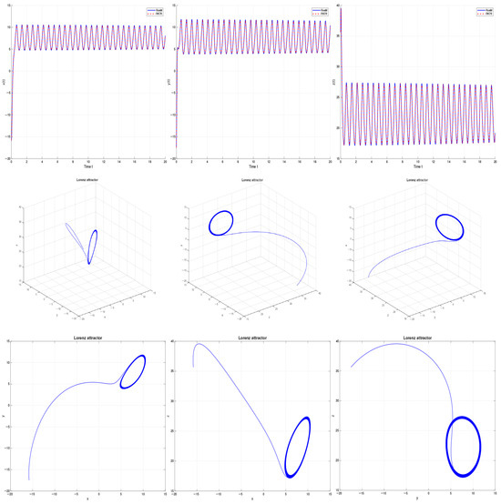
Figure 1.
Phase portraits using RosM for and .

Figure 2.
The absolute error for and .
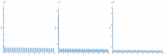
Figure 3.
The absolute error for and .
The step size for the numerical integration of the Lorenz system was determined through a comprehensive analysis that balanced four key factors: numerical stability, accuracy requirements, computational efficiency, and the preservation of chaotic properties. The step size plays a vital role in error control, stability maintenance, dynamics preservation, and resource management, ensuring accurate capture of chaotic behavior while maintaining computational feasibility for long-term simulations.
3.2. Chaotic Solutions
We consider the case with the other parameters as given above which exhibits chaotic solutions. In Table 2, differences between 10-term decomposition and RK78 solutions for , at various error tolerances are shown. In Figure 4, the approximate solution and . In Figure 5, the absolute error for and . In Figure 6, the absolute error for and . The elapsed time is 0.189868 s for and 1.406850 s for .
Table 2.
Absolute errors for chaotic regime () comparing RosM with ADM and MHPM. RosM maintains excellent accuracy throughout the simulation, while ADM and MHPM exhibit significant error growth over time, particularly beyond .
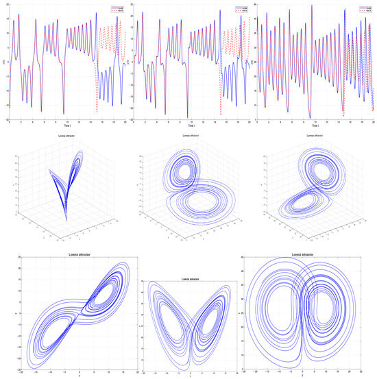
Figure 4.
Phase portraits using RosM for and .
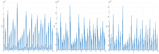
Figure 5.
The absolute error for and .
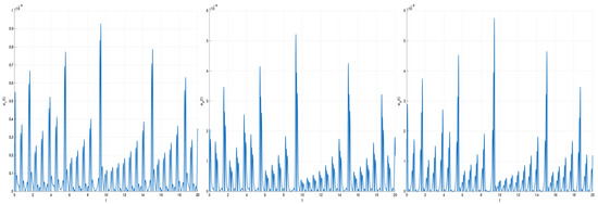
Figure 6.
The absolute error for and .
Table 2 reveals several key findings:
- RosM stability: The method maintains consistent accuracy throughout the chaotic regime, with errors remaining below even at .
- Comparative advantage: RosM significantly outperforms ADM and MHPM in long-term integration, where the semi-analytical methods exhibit exponential error growth.
- Step size sensitivity: Reducing h from to improves RosM accuracy by approximately three orders of magnitude, confirming robust convergence behavior.
3.3. Bifurcation Analysis
To further validate RosM’s capability for qualitative analysis, we generated bifurcation diagrams for the Lorenz system. The methodology involved:
- Parameter range: with
- For each R: integrate using RosM with , discard first 50 time units as transient
- Record local maxima of z variable for statistical analysis
- Compare with reference RK78 results
The bifurcation diagram obtained using RosM shows excellent agreement with that generated by the RK78 method (Figure 7), confirming that the RosM accurately captures the complex dynamical transitions of the Lorenz system. This demonstrates RosM’s capability not only for time integration but also for comprehensive dynamical analysis of nonlinear systems.
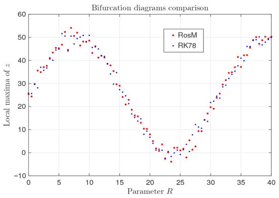
Figure 7.
Comparison of bifurcation diagrams generated by RosM (red) and RK78 (blue), showing excellent agreement across all dynamical regimes.
The generation of the bifurcation diagram further demonstrates RosM’s capability for comprehensive dynamical analysis. The method successfully captures all critical transition points and the complex structure of the chaotic attractor, providing a complete picture of the system’s behavior across parameter space. This makes RosM a valuable tool not only for time integration but also for qualitative analysis of nonlinear dynamical systems.
In Figure 8, Figure 9 and Figure 10, simulations were conducted with extended time horizons () to properly capture long-term chaotic behavior and ensure statistical significance. The elapsed time is 0.516269 s.
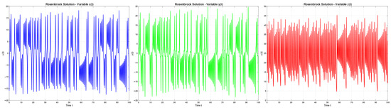
Figure 8.
Phase portraits using RosM for and .
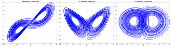
Figure 9.
Phase portraits using RosM for and .
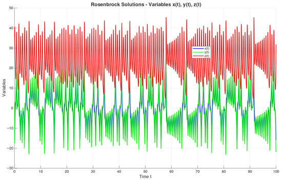
Figure 10.
Phase portraits using RosM for and .
For our study, we selected through systematic analysis, which provides an optimal balance between accuracy (global error ), stability, and computational efficiency, while faithfully preserving the chaotic properties of the Lorenz system.
This comprehensive approach ensures that our numerical results are both reliable and meaningful for the analysis of chaotic dynamics.
Now, we apply RosM of system in [24]:
with the parameters a and b being positive real numbers. For the parameters and being held constant and conditions initiales , utilizing the ode45 algorithm for , we have Figure 11 with simulation completed in 0.37 s for RosM and 0.23 s for ode45. Simplified bifurcation diagrams of the memristor system in Figure 12.
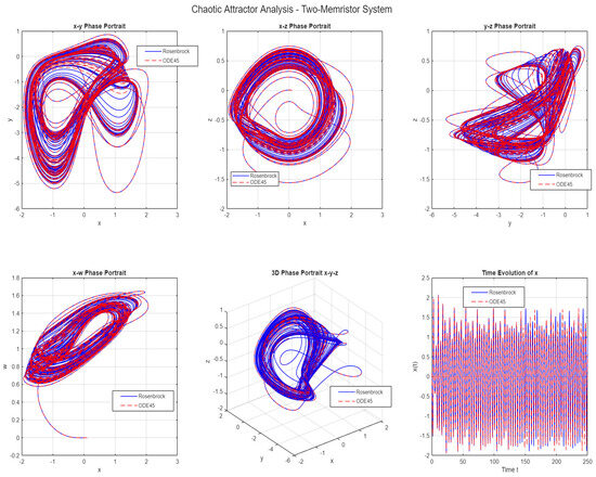
Figure 11.
Chaotic attractor of the two-memristor system using RosM and ode45 comparison. 3D phase space (x-y-w), x-y projection, time series of state variables.
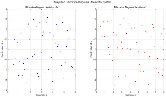
Figure 12.
Bifurcation analysis of the memristor system. Variation with parameter a, variation with parameter b, showing multistability and chaotic transitions.
3.4. Performance Analysis on Memristor System
The computational performance of the Rosenbrock method was evaluated on the two-memristor chaotic system. As shown in Figure 11, both RosM and ode45 successfully capture the complex chaotic dynamics, with RosM completing the simulation in 0.37 s compared to 0.23 s for ode45.
Execution Time Analysis:
- RosM: 0.37 s with fixed step size .
- ode45: 0.23 s with adaptive step sizing.
- Time ratio: RosM/ode45 = 1.61.
Performance Interpretation: The 61% additional computational time for RosM is attributed to its implicit structure requiring linear system solutions at each step. However, this cost brings significant advantages:
- Predictable performance: Fixed step size ensures consistent computation time
- Enhanced stability: L-stability prevents numerical instability in stiff regions
- Symmetry preservation: Maintains structural invariants crucial for long-term integration
Bifurcation Analysis: Figure 12 demonstrates RosM’s capability for qualitative dynamical analysis. The bifurcation diagrams reveal:
- Complex multistability regions as parameters a and b vary.
- Sudden transitions between periodic and chaotic behavior.
- Multiple coexisting attractors characteristic of memristor systems.
The method reliably captures these delicate dynamical features, confirming its suitability for comprehensive system analysis beyond mere time integration.
4. Conclusions
This research has successfully assessed the efficacy of the second-order Rosenbrock method (RosM) for numerical integration of the chaotic Lorenz system, including performance analysis against the RK78 method. It has been found that RosM clearly maintains accuracy for non-chaotic () and chaotic () cases, with orders of errors between – for , increasing to – for , while retaining stability in the resolution of complex chaotic dynamics. Compared to ADM and MHPM approaches, the RosM yields greater accuracy for the same parameters, showcasing strong accuracy potential. Our work provides methodological contributions by proposing the Rosenbrock method as an alternative method to high-order explicit methods for chaotic systems, tested through numerous numerical experiments in various dynamical regimes. We present practical advice for implementation and demonstrate the capabilities of the RosM to be used in qualitative analysis through bifurcation analysis. While the current findings have highlighted the reliability of long-time simulation of the Lorenz system, we will explore higher-order Rosenbrock methods, adaptive step-size control in chaotic regimes, implementation in other chaotic systems (Rössler, Chen), and using advanced linear algebra methods for improved computational efficiency. The implicit method provides a stable, reliable alternative that is particularly beneficial for stiff systems in nonlinear dynamical analyses. These findings confirm the Rosenbrock method is an effective method for simulating long-time simulations of the Lorenz system.
Beyond its application to the Lorenz system, the symmetry-preserving Rosenbrock method demonstrates considerable potential for broader scientific computing applications. In fluid dynamics, our approach could ensure conservation of fundamental symmetries in turbulent flow simulations, particularly for large-scale atmospheric and oceanic models. For plasma physics applications, the method’s ability to maintain structural invariants makes it suitable for long-term MHD simulations where symmetry breaking can lead to unphysical plasma behavior in fusion devices. In climate modeling, the reliable long-term integration properties of our method address critical needs for maintaining conservation laws in decade-scale climate projections. Future work will explore these application domains, particularly focusing on adaptive Rosenbrock methods for multi-scale physical systems where symmetry preservation is paramount for predictive accuracy.
Author Contributions
Methodology, L.S. and I.A.; Formal analysis, L.S. and I.A.; Software, L.S. and I.A.; Writing—original draft, L.S. and I.A.; Writing—review and editing, I.A. All authors have read and agreed to the published version of the manuscript.
Funding
This work was supported and funded by the Deanship of Scientific Research at Imam Mohammad Ibn Saud Islamic University (IMSIU) (grant number IMSIU-DDRSP2502).
Data Availability Statement
No new data were created or analyzed in this study. Data sharing is not applicable to this article.
Acknowledgments
This work was supported and funded by the Deanship of Scientific Research at Imam Mohammad Ibn Saud Islamic University (IMSIU) (grant number IMSIU-DDRSP2502).
Conflicts of Interest
The author declares no conflicts of interest.
References
- Adomian, G. Nonlinear Stochastic Systems Theory and Application to Physics; Kluwer Academic Publishers: Dordrecht, The Netherlands, 1989. [Google Scholar]
- Adomian, G. A review of the decomposition method in applied mathematics. J. Math. Anal. Appl. 1988, 135, 501–544. [Google Scholar] [CrossRef]
- Adomian, G. Solving Frontier Problems of Physics: The Decomposition Method; Kluwer Academic Publishers: Boston, MA, USA, 1994. [Google Scholar]
- Biazar, J.; Babolian, E.; Islam, R. Solution of the system of ordinary differential equations by Adomian decomposition method. Appl. Math. Comput. 2004, 147, 713–719. [Google Scholar] [CrossRef]
- Hashim, I.; Noorani, M.S.M.; Ahmad, R.; Bakar, S.A.; Ismail, E.S.; Zakaria, A.M. Accuracy of the Adomian decomposition method applied to the Lorenz system. Chaos Solitons Fractals 2006, 28, 1149–1158. [Google Scholar] [CrossRef]
- Biazar, J.; Montazeri, R. A computational method for solution of the prey and predator problem. Appl. Math. Comput. 2005, 163, 841–847. [Google Scholar] [CrossRef]
- Evans, D.J.; Raslan, K.R. The Adomian decomposition method for solving delay differential equations. Int. J. Comput. Math. 2005, 82, 49–54. [Google Scholar] [CrossRef]
- Hashim, I.; Noorani, M.S.M.; Al-Hadidi, M.R.S. Solving the generalized Burgers-Huxley equation using the Adomian decomposition method. Math. Comput. Model. 2006, 43, 1404–1411. [Google Scholar] [CrossRef]
- Kaya, D.; El-Sayed, S.M. Numerical soliton-like solutions of the potential Kadomtsev–Petviashvili equation by the decomposition method. Phys. Lett. A 2003, 320, 192–199. [Google Scholar] [CrossRef]
- Sadek, E.M.; Bentbib, A.H.; Sadek, L.; Talibi Alaoui, H. Global extended Krylov subspace methods for large-scale differential Sylvester matrix equations. J. Appl. Math. Comput. 2020, 62, 157–177. [Google Scholar] [CrossRef]
- Sadek, L. Fractional BDF methods for solving fractional differential matrix equations. Int. J. Appl. Comput. Math. 2022, 8, 238. [Google Scholar] [CrossRef]
- Fedoseev, P.; Pesterev, D.; Rozhkov, V.; Rybin, V.; Butusov, D. Chaotic Encryption Algorithm Based on Gingerbreadman Map with Adaptive Symmetry. Chaos Theory Appl. 2025, 7, 31–41. [Google Scholar] [CrossRef]
- Lorenz, E.N. Deterministic nonperiodic flow. J. Atmos. Sci. 1963, 20, 130–141. [Google Scholar] [CrossRef]
- Guellal, S.; Grimalt, P.; Cherruault, Y. Numerical study of Lorenz’s equation by the Adomian method. Comput. Math. Appl. 1997, 33, 25–29. [Google Scholar] [CrossRef]
- Olek, S. An accurate solution to the multispecies Lotka-Volterra equations. SIAM Rev. 1994, 36, 480–488. [Google Scholar] [CrossRef]
- Vadasz, P.; Olek, S. Convergence and accuracy of Adomian’s decomposition method for the solution of Lorenz equation. Int. J. Heat Mass Transf. 2000, 43, 1715–1734. [Google Scholar] [CrossRef]
- Répaci, A. Nonlinear dynamical systems: On the accuracy of Adomian’s decomposition method. Appl. Math. Lett. 1990, 3, 35–39. [Google Scholar] [CrossRef]
- Shawagfeh, N.; Adomian, G. Non-perturbative analytical solution of the general Lotka-Volterra three-species system. Appl. Math. Comput. 1996, 76, 251–266. [Google Scholar] [CrossRef]
- Shawagfeh, N.; Kaya, D. Comparing numerical methods for the solutions of systems of ordinary differential equations. Appl. Math. Lett. 2004, 17, 323–328. [Google Scholar] [CrossRef]
- Rosenbrock, H.H. Some general implicit processes for the numerical solution of differential equations. Comput. J. 1963, 5, 329–330. [Google Scholar] [CrossRef]
- Kaya, Y.; Aydin, Z.G. A Chaos-Based Encryption Scheme for Secure Medical X-ray Images. Comput. Electron. Med. 2025, 2, 53–59. [Google Scholar] [CrossRef]
- Noor, N.F.M.; Hashim, M.S.M.I. A note on the accuracy of the Adomian decomposition method applied to the chaotic Lorenz system. J. Comput. Appl. Math. 2010, 234, 1526–1533. [Google Scholar]
- Chowdhury, M.S.H.; Hashim, I.; Momani, S. The multistage homotopy-perturbation method: A powerful scheme for handling the Lorenz system. Chaos Solitons Fractals 2009, 40, 1929–1937. [Google Scholar] [CrossRef]
- Khan, A.; Li, C.; Zhang, X.; Cen, X. A two-memristor-based chaotic system with symmetric bifurcation and multistability. Chaos Fractals 2025, 2, 1–7. [Google Scholar] [CrossRef]
Disclaimer/Publisher’s Note: The statements, opinions and data contained in all publications are solely those of the individual author(s) and contributor(s) and not of MDPI and/or the editor(s). MDPI and/or the editor(s) disclaim responsibility for any injury to people or property resulting from any ideas, methods, instructions or products referred to in the content. |
© 2025 by the authors. Licensee MDPI, Basel, Switzerland. This article is an open access article distributed under the terms and conditions of the Creative Commons Attribution (CC BY) license (https://creativecommons.org/licenses/by/4.0/).