An Adaptive Learning Algorithm Based on Spiking Neural Network for Global Optimization

Abstract

The optimal computing ability of spiking neural networks (SNNs) mainly depends on the connection weights of their synapses and the thresholds that control the spiking. In order to realize the optimization calculation of different objective functions, it is necessary to modify the connection weights adaptively and make the thresholds dynamically self-learning. However, it is very difficult to construct an adaptive learning algorithm for spiking neural networks due to the discontinuity of neuron spike sending process, which is also a fatal problem in this field. In this paper, an efficient adaptive learning algorithm for spiking neural networks is proposed, which adjusts the weights of synaptic connections by a learning factor adaptively and adjusts the probability of spike sending by the self-organizing learning method of the dynamic threshold, so as to achieve the goal of automatic global search optimization. The algorithm is applied to the learning task of global optimization, and the experimental results show that this algorithm has good stability and learning ability, and is effective in dealing with complex multi-objective optimization problems of spatiotemporal spike mode. Moreover, the proposed framework explicitly leverages problem and model symmetries. In Traveling Salesman Problems, distance symmetry (d(i, j) = d(j, i)) and tour permutation symmetry are preserved by our spike-train-based similarity and energy updates, which do not depend on node labels. Together with the homogeneous neuron dynamics and balanced excitatory–inhibitory populations, these symmetry-aware properties reduce the effective search space and enhance the convergence stability.

1. Introduction

How to design an optimization tool based on the evolutionary principle of biological brain and apply it to the global optimization of objective function has become a hot topic in current research [1,2,3]. Adaptive learning spike neural networks are powerful computational intelligence tools for fast and efficient optimization of computation [4]. They exchange information in the form of precisely timed events [5,6,7]. The results of many studies show that the optimal performance of spiking neural networks is largely determined by the adaptive change in weights and the dynamic change in thresholds for complex application scenarios of objective functions [8,9,10].

For the adaptive learning algorithms of various neural networks, some studies have performed detailed research [11,12,13,14]. Jiang et al. [11] proposed an online learning algorithm based on a neural network and designed the weight update rate of a neural network based on the gradient descent method. Richert et al. [12] analyzed the influence of neural network in discrete time, studied the weight of a delta rule update applied to a relatively slow number rate, and this weight-update method can enable the neural network to estimate the discrete time model of the system, and solve the contradiction between the speed of the number rate and the size of neural networks. Shrestha et al. [13] used the adaptive learning rate rule based on the dead-zone switch to learn the continuous spike training in the spiking neural network with a hidden layer on the basis of the weight update strategy, so as to ensure the convergence of the learning process in the sense of weight convergence and the robustness of the learning process to the external interference. Lim et al. [14] investigated a learning rule based on the back-propagation algorithm for the hardware-based deep neural network. This adaptive learning rule can realize forward and backward propagation and weight update in the hardware, which is conducive to the implementation of an efficient and high-speed deep neural network. The traditional values of a neural network adaptive control method is not updated in a continuous time corresponding parameter adaptive control, and cannot be studied well by optimizing results from changes to adapt to the cumulative values. Therefore, it is worth considering that the cost function of the whole system changes by changing the weights through the occurrence probability of spikes, so as to approach the lowest point of the system consumption.

Inspired by the computational methods of biological neural networks, several adaptive learning rules based on spiking neural networks have been proposed recently [15,16,17]. Emelyanov et al. [15] applied spike–time-dependent plasticity (STDP) model rules to memory nanocomposite structures as synaptic weights. Such local spiking neural network learning rules established self-organizing information associations between presynaptic and postsynaptic neurons, which proved adaptive nonspecific and rate-coding pattern-specific learning of spike neurons. Pilly et al. [16] presented a neural model in which spike neurons operate in the hierarchy of self-organizing maps that amplify and learn to classify the most frequent and active symbiotic events they input. Based on the rate-based grid and location-based cell learning models, a rate-based adaptive neural model is described to transform its cells into spike dynamics models. Shrestha et al. [17] analyzed the weight convergence of the spiking neural network to determine the appropriate step size for each iteration of the weight update, and deduced the adaptive learning rate to be extended for the SpikeProp to ensure the convergence of the learning process. However, in view of the spike excitation characteristics of the spiking neural network, the self-organizing learning method of the dynamic threshold of the spiking neural network has not been well studied.

In this paper, based on the existing research [18,19,20,21,22], the adaptive learning algorithm of the spiking neural network is applied to global optimization, and its feasibility and effectiveness are verified by simulation. The remainder of this paper is organized as follows. The basic theory including the spiking neural network model and the simplification of the model are described in Section 2. Section 3 introduced the adaptive adjustment of synaptic connection weights and the self-organizing evolution method of the dynamic threshold for global optimization. In Section 4, the algorithm is used in the simulation experiments of global optimization. Finally, the conclusions are drawn in Section 5.

2. Spiking Neural Network Model and Its Model Simplification

2.1. Spiking Neural Network Model

In essence, the spiking neural network (SNN) is a single-layer neural network that does not require training [23,24,25]. Several spiking neurons connected together can form an optimized processing system based on the SNN [26]. The structural model of a single spiking neuron is shown in Figure 1.

It can be seen from the above neuron structure model that the internal activity intensity $V_i\left(t\right)$ of the neuron i can be expressed as

$$V_i\left(t\right)=e^{-\alpha }{V}_i(t-1)+\sum _{j=1}^n{W}_{ji}{Y}_j\left(t\right)+b_i$$

(1)

where j and i are the presynaptic neuron and the postsynaptic neuron, and n represents the total number of presynaptic input neurons. $\alpha$ represents the attenuation factor. $V_i(t-1)$ represents the internal activity intensity at the previous time. $W_{ji}$ is the connection weight between the neuron j and the neuron i, which can realize the transmission of ignition information among neighborhood neurons. $Y_j\left(t\right)$ is the spike train from the neuron j, and $b_i$ represents the bias.

If the internal activity intensity $V_i\left(t\right)$ of the neuron is greater than the dynamic threshold $V_{\theta }\left(t\right)$, then the neuron will fire and generate spikes at the same time, that is

$$Y_i\left(t\right)=S(V_i\left(t\right)-V_{\theta }\left(t\right))$$

(2)

where $S(\ast )$ is the unit step function.

The dynamic threshold $V_{\theta }\left(t\right)$ can be expressed as

$$V_{\theta }\left(t\right)=e^{-{\alpha }_{\theta }}{V}_{\theta }(t-1)+A_{\theta }{Y}_i\left(t\right)$$

(3)

where ${\alpha }_{\theta }$ and $A_{\theta }$ are the attenuation factor and the amplification factor of the dynamic threshold $V_{\theta }$, respectively.

According to Equation (2), it can be found that after neuron i fires, the dynamic threshold will cause $A_{\theta }$ to increase instantaneously. The attenuation factor ${\alpha }_{\theta }$ decays the threshold exponentially until the next firing of the neuron.

The firing frequency of the spiking neurons is constant, and the current firing neurons will stimulate the synchronous oscillation of the neighborhood similar neurons [27], that is, a neuron will fire to find the nearby similar neurons and make them fire synchronously, which is the reason why the spiking neural network can achieve global optimization.

2.2. Model Simplification

Spiking neural network model has many parameters which have great influence on global optimization [21]. In order to facilitate global adaptive optimization, the initial SNN model needs to be simplified, that is

$$V_i\left(t\right)=\sum _{j=1}^n{W}_{ji}{Y}_j\left(t\right)$$

(4)

$$Y_i\left(t\right)=V_i\left(t\right)>V_{\theta }(t-1)$$

(5)

$$V_{\theta }\left(t\right)=A_{\theta }H(V_i\left(t\right)-g)$$

(6)

where g represents the optimization standard value of firing $\left\{i\right|Y_i(t-1)=1\}$.

In Equation (6), H represents a smooth step function, that is the Heaviside step function [28], which can usually be expressed as

$$H\left(x\right)\approx {\displaystyle \frac{1}{2}}+{\displaystyle \frac{1}{2}}tanh\gamma x={\displaystyle \frac{1}{1+e^{-2\gamma x}}}$$

(7)

where a larger $\gamma$ corresponds to a sharper transition at $x=0$.

If we just think about the input and output of the single spiking neuron. The input and output of the spiking neuron are expressed in the form of spike trains, that is, spike trains encode neural information or external stimulus signals. The input spike trains of the presynaptic neuron is $Y_j$, the output spike train of the postsynaptic neuron is $Y_i$. The relation between the input spike train $Y_j$ and output spike train $Y_i$ at time t is expressed as a linear combination relation,

$$l_{Y_i}\left(t\right)=\sum _{j=1}^n{W}_{ji}{l}_{Y_j}\left(t\right)$$

(8)

Remark 1.

When the spike trains are expressed as a linear combination relationship, corresponding learning rules can be constructed to adjust the connection weights of spiking neurons. If $l_Y\left(t\right)$ is interpreted as the density function of the spike trains over time, the density function of the postsynaptic spike train can be expressed as a linear combination of the density function of the presynaptic spike trains for the generalized linear neuron model.

Remark 2.

Compared with the structural model of the single spiking neuron before simplification, the output spike train depends only on the weights W between the input spike trains of the neighborhood neurons, and the dynamic threshold $V_{\theta }\left(t\right)$ is only related to the amplification factor $A_{\theta }$. Therefore, the system optimization only needs to consider the two main parameters W, $A_{\theta }$ of the simplified SNN model as optimization objects.

3. Adaptive Learning Algorithm for Spiking Neural Networks

It can be seen from the above analysis that the spiking is probabilities [29], and because of this probability, spikes may be generated at any time [30]. With each redistribution, the synaptic connection weights W will be changed, which makes the cost function change every time [31]. If the synaptic connection weights are adjusted adaptively through the occurrence probability of spikes, so that the cost function always develops towards the low consumption state, then the global optimization of the system can be realized eventually.

In addition, the probability of spiking is largely dependent on the dynamic threshold. Therefore, the self-learning method of SNN dynamic threshold is particularly important.

3.1. Adaptive Adjustment for Synaptic Connection Weights

The key to construct the adaptive learning algorithm of spiking neural networks is to define the cost function of spike trains and the learning rules of connection weights [32].

All connection weights are adjusted using the delta update rule. The connection weight $W_{ji}$ from presynaptic neuron j to postsynaptic neuron i is expressed as

$$W_{ji}(t+1)=W_{ji}\left(t\right)+\mathrm{\Delta }{W}_{ji}+\xi \left(t\right)$$

(9)

where $\mathrm{\Delta }{W}_{ji}=-\eta \nabla C_i$, $\eta$ represents the learning rate and $\xi \left(t\right)$ represents the random disturbance. $\nabla C_i$ represents the gradient value calculated by the cost function C of spike trains against the connection weight $W_{ji}$, which can be expressed as the integral of the derivative of the cost function $C\left(W_{ji}\left(t\right)\right)$ for the weight $W_{ji}\left(t\right)$ in the time interval T.

$$\nabla C_i={\int }_T{\displaystyle \frac{𝜕C\left(W_{ji}\left(t\right)\right)}{𝜕W_{ji}\left(t\right)}}dt$$

(10)

We use the residual energy [33] to express the cost function, that is, the difference between the real energy obtained by the spike trains optimized by the adaptive learning algorithm and the expected energy of the spike trains.

$$C\left(W_{ji}\left(t\right)\right)=E_i\left(W_{ji}\left(t\right)\right)-E_e\left(W_{ji}\left(t\right)\right)$$

(11)

where $E_i\left(W_{ji}\left(t\right)\right)$ represents the optimized system energy [18], which has the following form

$$E=(1+\sigma )e^{{\displaystyle \frac{{(\mathrm{\Delta }t-\kappa )}^{2}ln\left(\frac{\sigma }{1+\sigma }\right)}{{\upsilon }^2}}}-\sigma$$

(12)

where $\sigma >0$ is a positive shape parameter that influences the “curvature” and baseline of the energy function. It tunes how the energy changes with other variables (e.g., time delays). $\kappa <0$ is a negative shape parameter that shifts the energy function’s response to time delays ($\mathrm{\Delta }t$). It helps define a reference point for $\mathrm{\Delta }t$, shaping how energy scales as $\mathrm{\Delta }t$ deviates from this reference. $\upsilon$ is a scaling parameter that controls the “sensitivity” of energy to changes in $\mathrm{\Delta }t$. Smaller v makes energy more responsive to $\mathrm{\Delta }t$ variations; larger v smooths this response. $E_e\left(W_{ji}\left(t\right)\right)$ represents the expected value of minimum energy (the global optimal solution). The cost function C reflects the difference between the solution obtained by the algorithm and the global optimal solution, and it must converge to a certain minimum value in a certain period of time to ensure that the network can obtain the optimal solution.

For the learning rule of connection weights, the concept of residual energy and the chain rule [34] are applied. According to Equations (8) and (11), the change amount of cost function C at time t can be deduced as

$${\displaystyle \frac{𝜕C\left(W_{ji}\left(t\right)\right)}{𝜕W_{ji}\left(t\right)}}={\displaystyle \frac{𝜕C\left(W_{ji}\left(t\right)\right)𝜕l_{Y_i}\left(t\right)}{𝜕l_{Y_i}\left(t\right)𝜕W_{ji}\left(t\right)}}=[l_{Y_i}\left(t\right)-l_{Y_e}\left(t\right)]l_{Y_j}\left(t\right)$$

(13)

where $l_{Y_i}\left(t\right)$ represents the input spike train, $l_{Y_j}\left(t\right)$ represents the output spike train and $l_{Y_e}\left(t\right)$ represents the expected spike train.

According to Equation (10), the adjustment of the synaptic connection weight $W_{ji}$ is calculated as

$$\nabla C_i={\int }_T[l_{Y_i}\left(t\right)-l_{Y_e}\left(t\right)]l_{Y_j}\left(t\right)dt=L(Y_i,Y_j)-L(Y_e,Y_j)$$

(14)

According to the derivation process discussed above, we present an adaptive synaptic learning rule based on spiking neurons, which is expressed as

$$\begin{array}{cc}\hfill \mathrm{\Delta }{W}_{ji}=& -\eta [L(Y_i,Y_j)-L(Y_e,Y_j)]\hfill \\ \hfill =& \eta [\sum _{e=1}^{n_e}\sum _{j=1}^{n_j}\epsilon (t_e,t_j)-\sum _{i=1}^{n_i}\sum _{j=1}^{n_j}\epsilon (t_i,t_j)]\hfill \end{array}$$

(15)

where $t_j$, $t_i$ and $t_e$ denote the issuing time of the corresponding spikes in the input spike train $Y_j$, the actual output spike train $Y_i$ and the expected spike train $Y_e$, respectively. $n_j$, $n_i$ and $n_e$ represent the total number of neuron input spike train $Y_j$, actual output spike train $Y_i$ and expected spike train $Y_e$, respectively. $\epsilon ({\ast }_1,{\ast }_2)$ represents the kernel function of the spike trains, which can be expressed as

$$\epsilon ({\ast }_1,{\ast }_2)=e^{{\displaystyle \frac{{\ast }_1-{\ast }_2}{\rho }}}$$

(16)

where the kernel function in exponential form defines the Hebbian term determined by the STDP (Spike Timing Dependnt Plasticity) mechanism [35], and the time constant $\rho =5ms$ is suitable in this paper.

Then, the adaptive learning rule for synaptic connection weights can be described as a combination of an “attenuation mechanism” and time:

$$\mathrm{\Delta }{W}_{ji}=\eta [\sum _{e=1}^{n_e}\sum _{t_j<t_e}{e}^{-{\displaystyle \frac{t_e-t_j}{\rho }}}-\sum _{i=1}^{n_i}\sum _{t_j<t_i}{e}^{-{\displaystyle \frac{t_i-t_j}{\rho }}}]$$

(17)

Remark 3.

The value of learning rate has a great influence on the convergence speed of the learning process and directly affects the calculation time and optimization efficiency. If the learning rate is too small and the effective update value of the weights in each iteration is too small, the convergence speed of the synaptic connection weights will be slow. On the contrary, it is easy to make the evolution process oscillate, affect the convergence speed of the network, and even lead to optimization failure. Adaptively adjusting the learning rate according to the probability of actual neuron firing can improve the adaptability of the learning algorithm to synaptic weights training.

In this paper, an learning factor $\beta$ is defined to make the learning rate $\eta$ of the connection weights adaptively adjust according to different spiking probability. According to the Gibbs sampling principle [36], the learning factor $\beta$ randomly circulates sampling in the d-dimensional sampling space until it is adjusted to an appropriate value, so as to obtain the optimal learning rate ${\eta }^{*}$. The d-dimensional Gibbs sampling algorithm for the learning factor $\beta$ is shown in Algorithm 1.

$${\beta }_d^{\left(t\right)}\sim p\left({\beta }_d\right|{\beta }_1^{\left(t\right)},{\beta }_2^{\left(t\right)},\dots ,{\beta }_d^{\left(t\right)})$$

(18)

Algorithm 1 d-dimensional Gibbs sampling algorithm for the learning factor $\beta$

Step 1 Random initialization $\{{\beta }_k:k=1,2,\dots ,d\}$

Step 2 Sampled cyclically with $t=0,1,2,\dots$

1. ${\beta }_1^{(t+1)}\sim p\left({\beta }_1\right|{\beta }_2^{\left(t\right)},{\beta }_3^{\left(t\right)},\dots ,{\beta }_d^{\left(t\right)})$

2. ${\beta }_2^{(t+1)}\sim p\left({\beta }_2\right|{\beta }_1^{(t+1)},{\beta }_3^{\left(t\right)},\dots ,{\beta }_d^{\left(t\right)}$

3. …

4. ${\beta }_k^{(t+1)}\sim p\left({\beta }_k\right|{\beta }_1^{(t+1)},\dots ,{\beta }_{k-1}^{(t+1)},{\beta }_{k+1}^{\left(t\right)},\dots ,{\beta }_d^{\left(t\right)}$

5. …

6. ${\beta }_d^{(t+1)}\sim p\left({\beta }_d\right|{\beta }_1^{(t+1)},{\beta }_2^{(t+1)},\dots ,{\beta }_d^{(t+1)})$

According to the value of the learning factor $\beta$ in the learning interval $[{\beta }_{min},{\beta }_{max}]$, the adaptive adjustment mode of learning rate $\eta$ is as follows:

$$\eta =\left\{\begin{array}{c}\hfill {\displaystyle \frac{\beta -{\beta }_{min}}{{\beta }_{max}-{\beta }_{min}}},\beta <{\beta }_{min}\\ \hfill {\displaystyle \frac{{\beta }_{max}-\beta }{{\beta }_{max}-{\beta }_{min}}},\beta >{\beta }_{max}\end{array}\right.$$

(19)

According to Equation (16), we can know that the weights of synaptic connection are actually determined by two factors. In addition to the influence of learning rate, it is also related to the Euclidean distance between neurons, which is in line with the activity mechanism of link conduction between neurons through synapses in biology [37].

In the learning process of neuron’s spike trains, the evaluation of its learning performance is to judge the degree to which the actual issued spike train is close to the expected output spike train at the end of learning, which is actually to measure the similarity between the two spike trains. The actual output spike train $Y_i$ and the expected output spike train $Y_e$ satisfy Cauchy–Schwarz inequality [38] in the probability space, that is, $Y_i$ and $Y_e$ are arbitrary random variables in the probability space, then the covariance inequality is given by

$$Var{Y}_e\ge {\displaystyle \frac{Cov{(Y_e,Y_i)}^2}{Var\left(Y_i\right)}}$$

(20)

After defining an inner product on the set of random variables using the expectation of their product, $\langle Y_i,Y_e\rangle :=X\left(Y_i{Y}_e\right),$ the Cauchy–Schwarz inequality of spike trains in the probability space are expressed as

$$|X\left(Y_i{Y}_e\right){|}^2\le X\left(Y_i^2\right)X\left(Y_e^2\right)$$

(21)

We use Equation (20) to define the similarity measure F of two spike trains, which is represented as

$$F={\displaystyle \frac{\langle l_{Y_i}\left(t\right),l_{Y_i}\left(t\right)\rangle }{\parallel l_{Y_i}\left(t\right)\parallel \parallel l_{Y_i}\left(t\right)\parallel }}={\displaystyle \frac{L(Y_i,Y_e)}{\sqrt{L(Y_i,Y_i)}\sqrt{L(Y_e,Y_e)}}}$$

(22)

where $\parallel l_Y\left(t\right)=\sqrt{\langle l_Y\left(t\right),l_Y\left(t\right)\rangle }\parallel$ is the Euclidean norm of the spike trains. When the two spike trains are exactly the same, the value of F is 1, and as their similarity decreases, F gradually approaches 0.

Remark 4.

Several neuroscience theories have demonstrated the role of STDP in the long-term strengthening of synapses [39,40,41], which is the basis for the formation and learning of long-term memories in the brain. However, SNN learning with STDP alone will cause information loss when it tries to learn quickly to cope with the changing environment [32]. Memory persistence is a particular concern of SNN adaptive weights, however any pre/post synaptic sequence of STDP in the general form can modify the synapse, potentially erasing the previous information. The learning rule proposed in this paper combines the “attenuation mechanism” with time (Equation (16)) to solve the problem of information loss and stability-plasticity based on the weight updating process. Meanwhile, the Gibbs sampling principle is applied to the representation of learning rate to realize the adaptive adjustment of connection weights.

Remark 5.

The dynamic threshold mechanism may offer better temporal and spatial scalability compared to STDP-based methods. STDP-based threshold adaptation can be limited by the strict spike-timing requirements and the local synaptic interactions. Our dynamic mechanism, however, can be designed to operate at different time scales (from fast, real-time adjustments during path exploration to slower, long-term adaptations for overall system optimization) and across different spatial scales (from individual neuron thresholds to population-level threshold coordination). This allows for more flexible and efficient operation in large-scale, complex systems like the path planning for autonomous agents in a dynamic environment, where STDP-based methods may struggle to scale due to their inherent dependence on local, fine-grained spike-timing correlations.

3.2. The Self-Organized Learning Method of SNN Dynamic Threshold

Conventional SNN dynamic threshold is usually adjusted in a fixed proportion or a fixed step size, so as to facilitate the analysis and calculation of the optimization characteristics of SNN [42], but it also brings two problems:

• The rate of convergence to an optimal result is not ideal.
• It is easy to cause local extreme values or over-optimization phenomena.

Aiming at addressing these shortcomings, a two-dimensional Renyi entropy [43] method is proposed to determine the amplification factor of dynamic threshold, so that SNN can quickly converge to the optimal result, while avoiding local extreme value or over-optimization phenomenon.

Entropy can be used to quantitatively measure the amount of information in a system. Suppose a system has m possible states, and the probability density distribution of each state is $p_i$, where $i=\{1,2,\dots ,m\}$, then the entropy of the system (i.e., Gibbs entropy [44]) is defined as

$$R=-\sum _i^m{p}_{i}ln{p}_i$$

(23)

Renyi entropy is a generalized form of Gibbs entropy, which can provide flexible information measurement for hybrid or non-additive systems [43]. Therefore, Renyi entropy is more suitable to evaluate the information in the optimization process than traditional Gibbs entropy [45]. Renyi entropy is defined as

$$R={\displaystyle \frac{1}{1-\lambda }}ln\sum _i^m{p}_i^{\lambda }$$

(24)

where $\lambda$ is the order of Renyi entropy, and when $\lambda =1$, Renyi entropy is equivalent to Gibbs entropy. In general, Renyi entropy can be calculated with the help of the optimized objective function, but the objective function only reflects the spatial information of the probability distribution of the input variables [46]. Therefore, constraints in the optimization will interfere with the calculation of Renyi entropy, thus affecting the accuracy of the objective optimization [47].

In order to solve this problem, an information measurement method based on two-dimensional Renyi entropy is proposed. Assuming that after a SNN operation, the spike trains are divided into the actual output spike train $Y_i$ and the input spike train $Y_j$, then the two-dimensional Renyi entropy of the optimization process can be defined as $R=R_i+R_j$, where $R_i$ and $R_j$ are the two-dimensional Renyi entropy of the actual output spike train $Y_i$ and the input spike train $Y_j$, respectively, which can be defined as

$$R_i={\displaystyle \frac{1}{1-\lambda }}ln\sum _i\sum _j{\left[p_i(i,j)\right]}^{\lambda }$$

(25)

$$R_j={\displaystyle \frac{1}{1-\lambda }}ln\sum _i\sum _j{\left[p_j(i,j)\right]}^{\lambda }$$

(26)

where $p_i$ and $p_j$ are the two-dimensional joint probability density distributions of the actual output spike train $Y_i$ and the input spike train $Y_j$, respectively. The joint probability density calculation method can effectively deal with the effects of different constraints on the objective function, so that the two-dimensional Renyi entropy has a better global optimization performance.

The optimal result of global optimization has the most information, so the maximum two-dimensional Renyi entropy criterion of SNN for the optimization process can be determined. The amplification factor of dynamic threshold can be defined as

$$A_{\theta }=\mu {\displaystyle \frac{𝜕R}{𝜕t}}$$

(27)

where $\mu$ is the rate coefficient, t is the running time of SNN.

Remark 6.

In this paper, a method of dynamically adjusting the threshold of neurons is proposed to reflect the tightness of the spatial distribution between the actual output spike trains and the input spike trains. The maximum two-dimensional Renyi entropy criterion is used to establish the threshold amplification factor of the spiking neuron, which ensures that the optimal result of global optimization has the most information.

4. Simulation and Discussion

The adaptive learning algorithm can be applied to all kinds of global optimization problems because of its good learning ability and applicability. In this paper, we first analyze the feasibility, stability and robustness of the adaptive learning algorithm in the SNN model. Then, we take the two-dimensional shortest path optimization as an example to verify the effectiveness and global optimization performance of the proposed adaptive learning algorithm.

4.1. Stability and Robustness Verification

We first conduct an in-depth analysis of the stability of the simplified SNN model under the same conditions, whether without or with the use of the adaptive learning algorithm. Then, we demonstrate the robustness of the adaptive learning algorithm under different stimulus spikes and model parameters. All the simulations were performed from $t=0$ to $t=30$ units with a time step of 0.1 units.

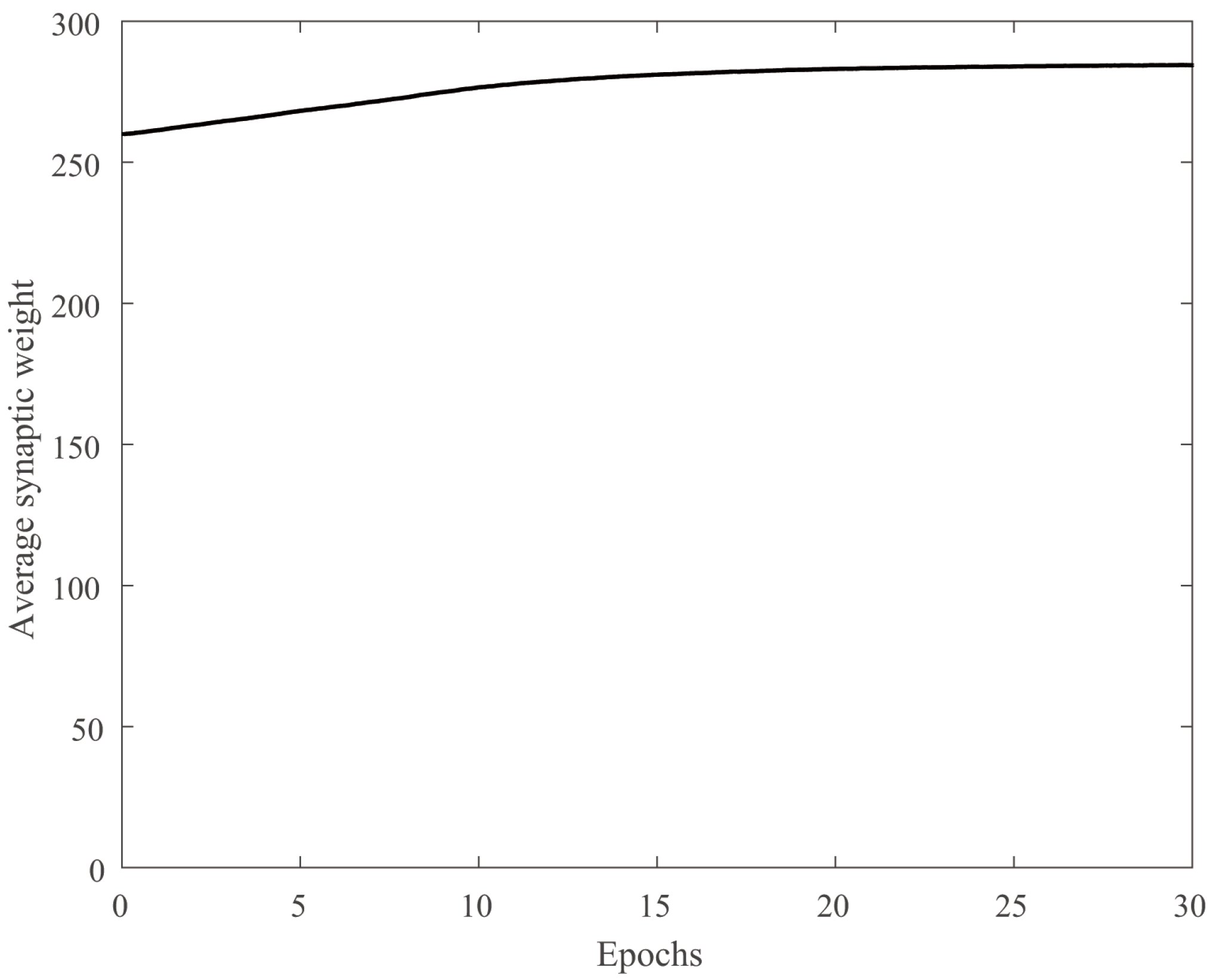
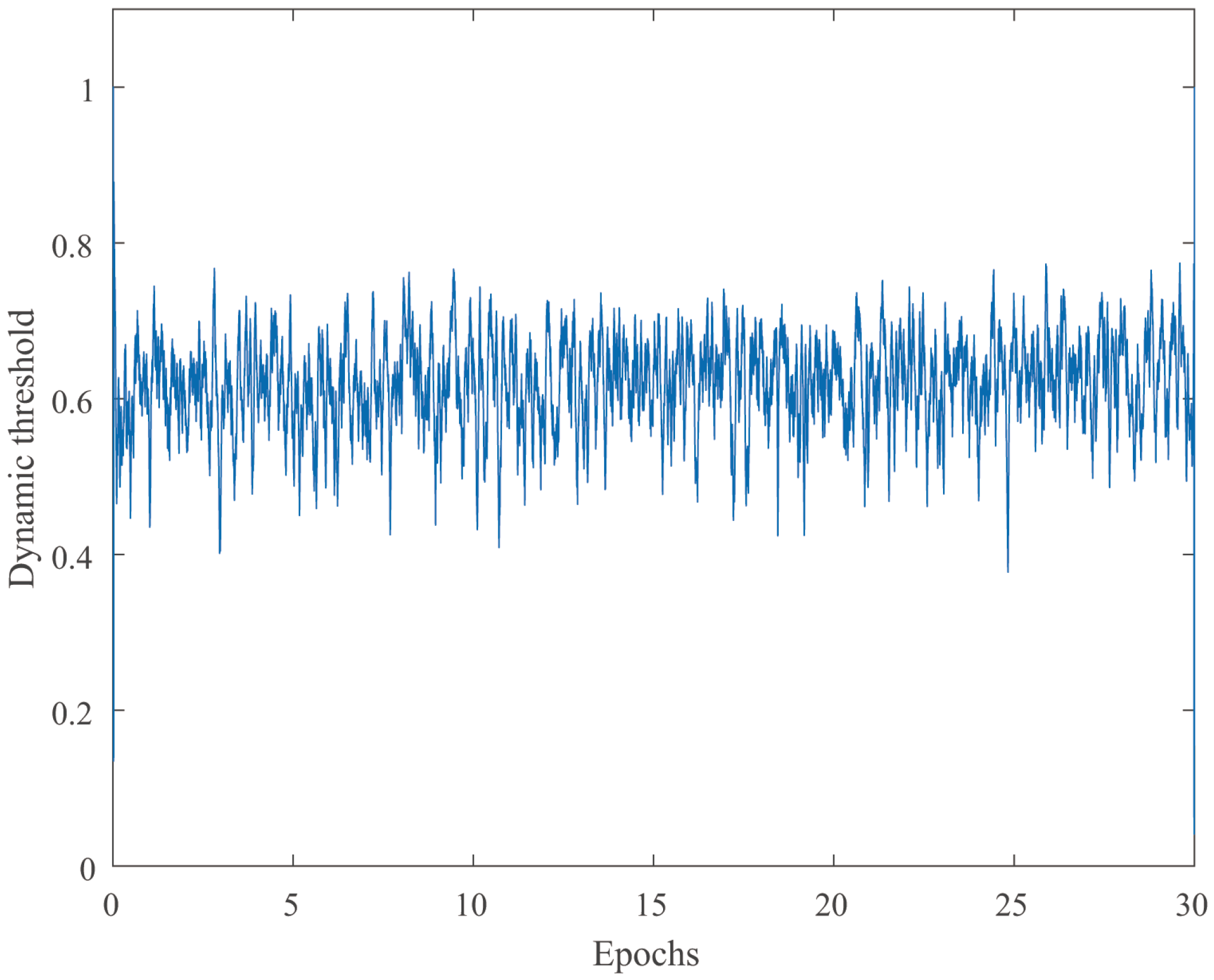
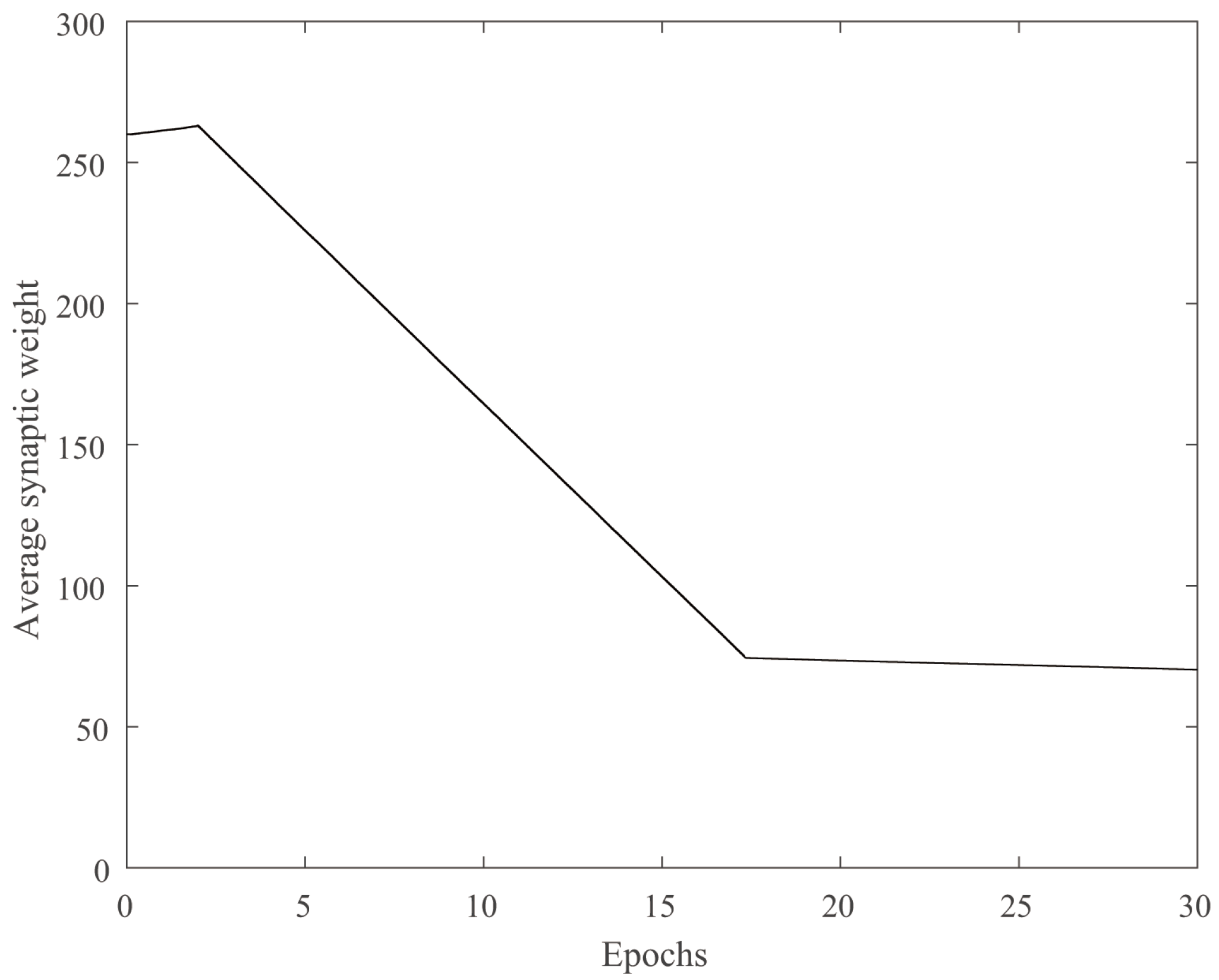
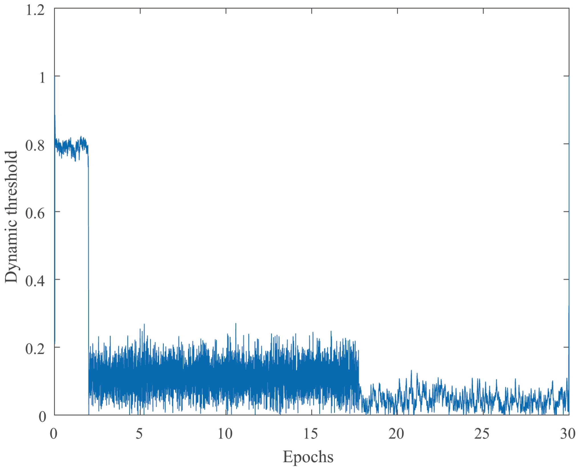
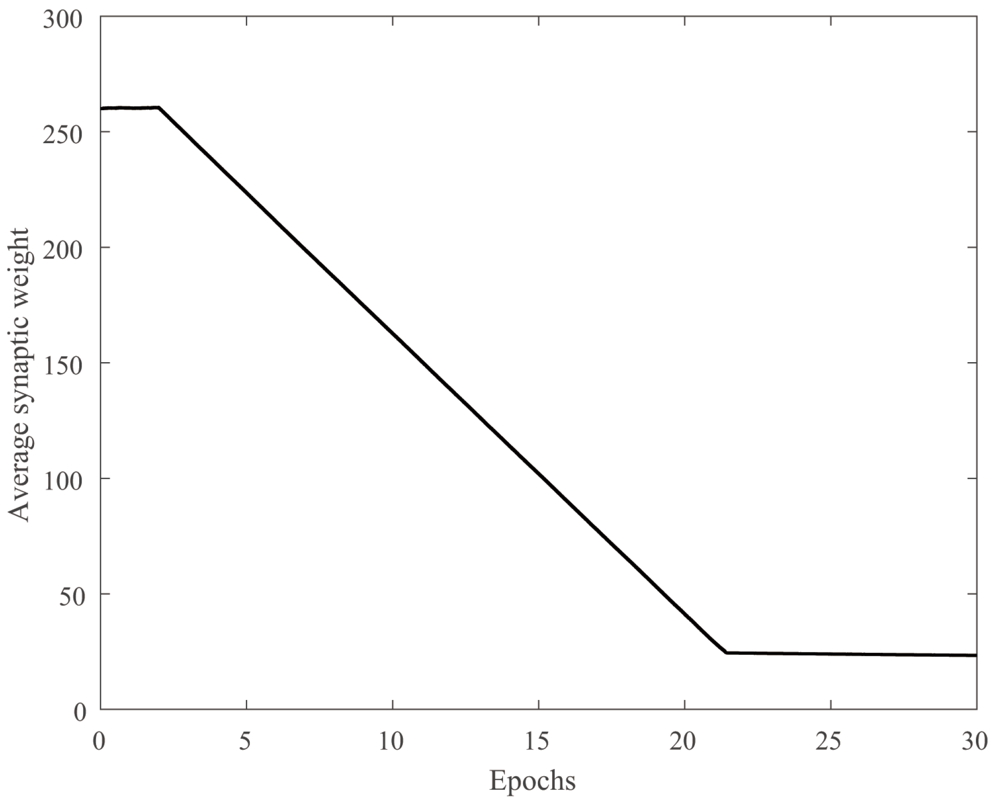
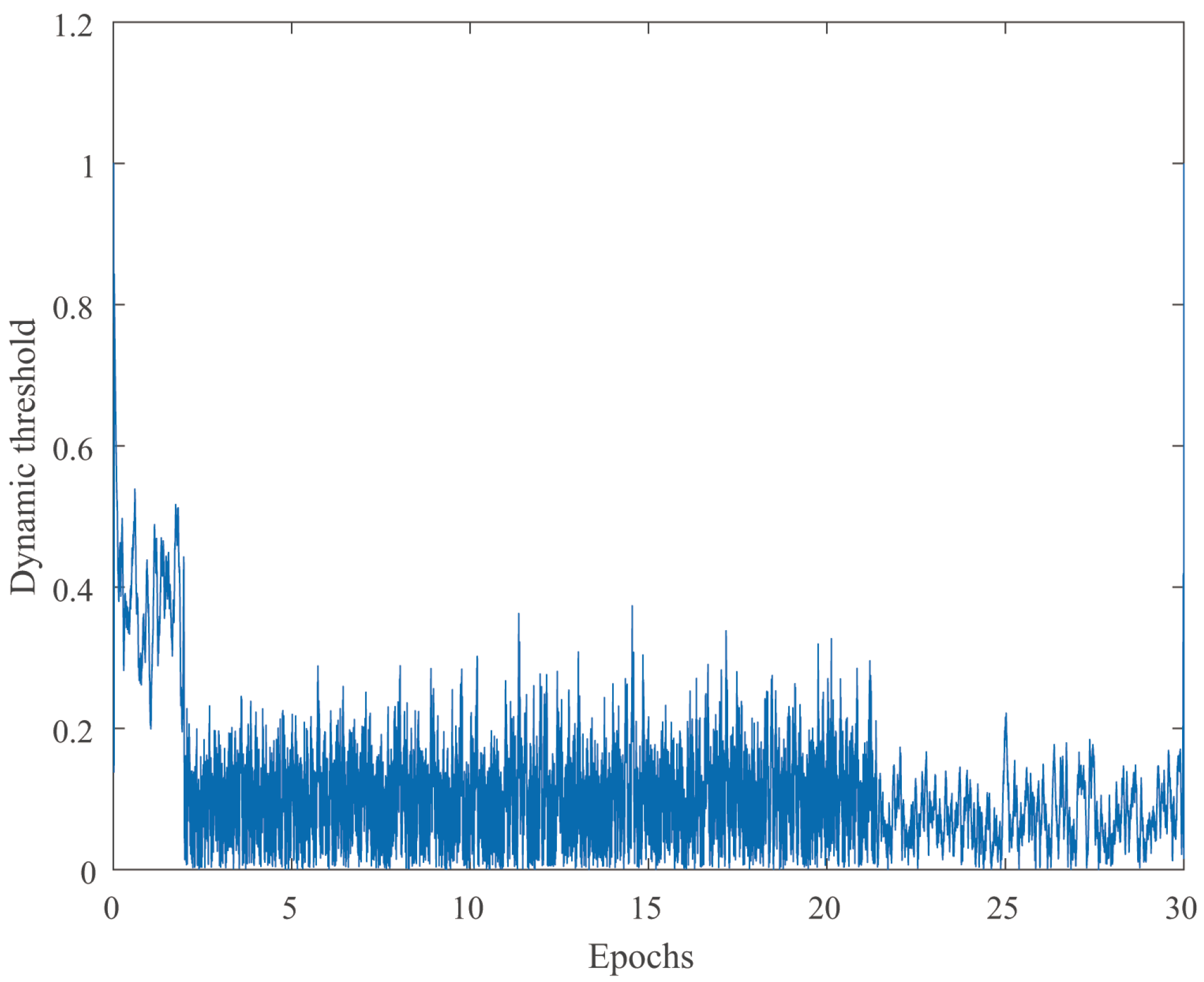
The adaptive learning algorithm is applied to the simplified SNN model, consisting of 100 excitatory neurons and 100 inhibitory neurons, to prove that our algorithm can be used to control the stability of neuron activity in the SNN. In the absence of an adaptive learning algorithm, the weight convergence and threshold changes in the simplified SNN model are shown in Figure 2 and Figure 3. The weight convergence and threshold changes in the simplified SNN model using the adaptive learning algorithm are shown in Figure 4 and Figure 5. It can be observed from Figure 2 and Figure 3 that, at the end of the 30th epoch, the SNN model without the adaptive learning algorithm still has no good convergence result for its weight value, so it must need more computing time to achieve convergence. Moreover, in this model, the dynamic threshold only changes periodically and repeatedly, and does not change dynamically according to the actual input spike trains. As can be seen from Figure 4 and Figure 5, the weight has converged to a relatively ideal result at the 17th epoch, and there will be no greater mutation. The dynamic threshold will also change with the convergence of the weights. Therefore, it can be concluded that the adaptive learning algorithm proposed by us can effectively converge and achieve a relatively stable state.

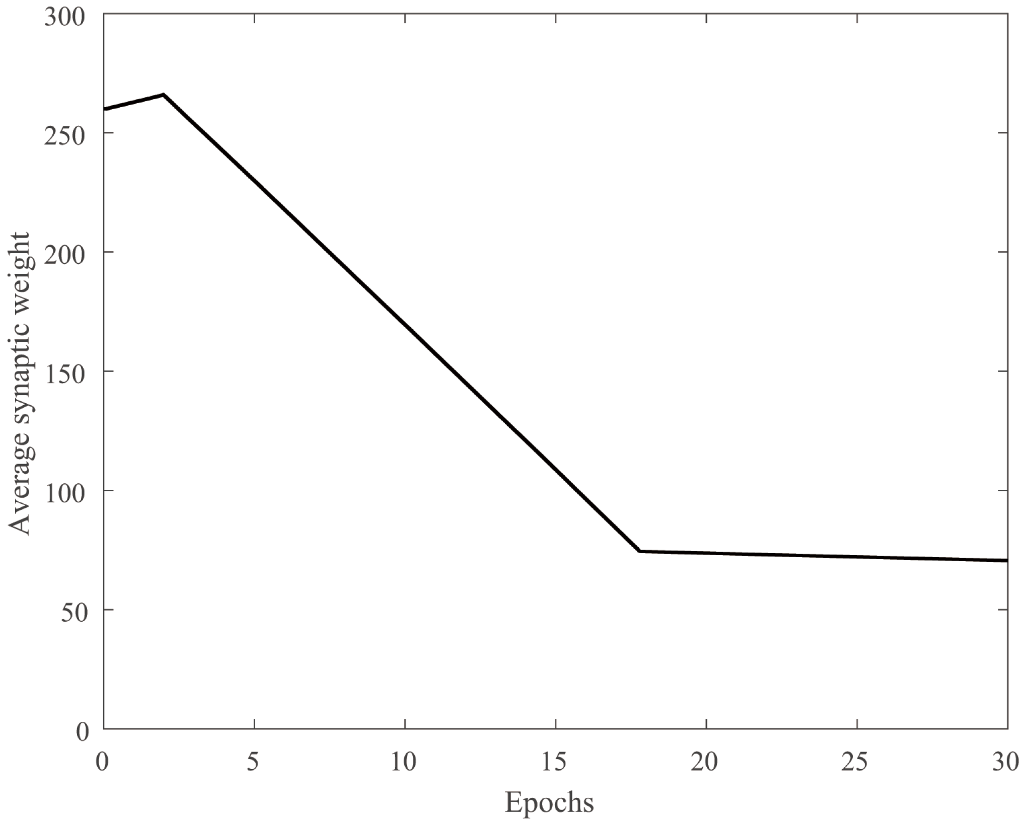
Next, we choose to simulate the proposed adaptive learning algorithm in a large SNN model (1000 neurons, half of which are excitatory neurons and half of which are inhibitory neurons). We can conclude that the calculation time will be longer in the case of more neurons, but the network weights can converge stably at the 18th epoch as shown in Figure 6, and the threshold also change dynamically, as shown in Figure 7. It is worth noting that since the network has an “attenuation mechanism” that converges to a lower average synaptic weight, we only need enough input to drive the network to a threshold to obtain output spike trains. In addition, according to the accumulation of different input spike trains, the threshold will also change accordingly, so as to ensure the robustness of the SNN model. Therefore, the dynamic change in the threshold is crucial.

In order to prove the robustness of the proposed algorithm in the SNN model, we selected a SNN model with 200 neurons (150 excitatory neurons and 50 inhibitory neurons) to show whether the SNN model would be very sensitive to the initial input in the case of different stimulus spikes, resulting in the instability of the model. As shown in Figure 8, the adaptive learning algorithm effectively controls the convergence of weights by driving the network weights into the “attenuation mechanism”. Figure 9 shows that the threshold is not greatly affected by the change in the initial value, but can still adapt to the spike trains of different input neurons well, so that the threshold can be self-organized and dynamically adjusted.

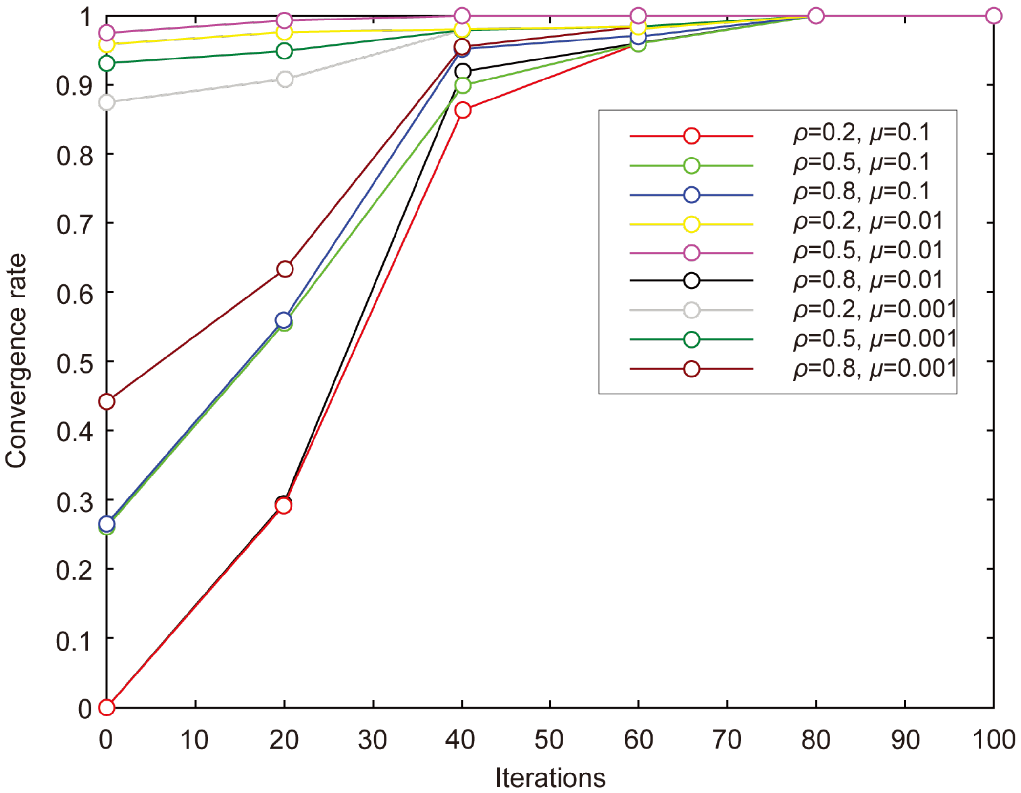
We demonstrate the robustness of our adaptive learning algorithm to the parameter uncertainties of SNN models. To prove this, we consider the effects of two parameters in the network on the convergence rate of the cost function C, namely the time constant $\rho$ of the neuron and the rate coefficient $\mu$ of the dynamic threshold amplification factor. We randomly assigned the time constant $\rho$ at first, and then locked its value range to 0.1∼0.9 as appropriate. Therefore, 0.2, 0.5 and 0.8 were selected as candidates for the experiment in this paper. The rate coefficient $\mu$ of the dynamic threshold amplification factor is also tested at 0.1, 0.01 and 0.001. In the experiments, as we can see from Figure 10, the convergence rate of the algorithm is the fastest and most stable when $\rho =0.5$ and $\mu =0.01$. All experiments ran 100 iterations.

4.2. Traveling Salesman Problem

In order to verify the advantages of the proposed algorithm in the application of global optimization, we applied the SNN model with an adaptive learning algorithm to a two-dimensional path optimization problem. The Traveling Salesman Problem (TSP) is a classical path planning problem [48]. SNN optimization algorithm has been applied to TSP, but no adaptive learning algorithm is used. Therefore, we compare the effect of SNN applied to TSP without an adaptive learning algorithm (SNN(O)) and SNN applied to TSP with an adaptive learning algorithm (SNN(A)), and their relevant parameters are set to the same.

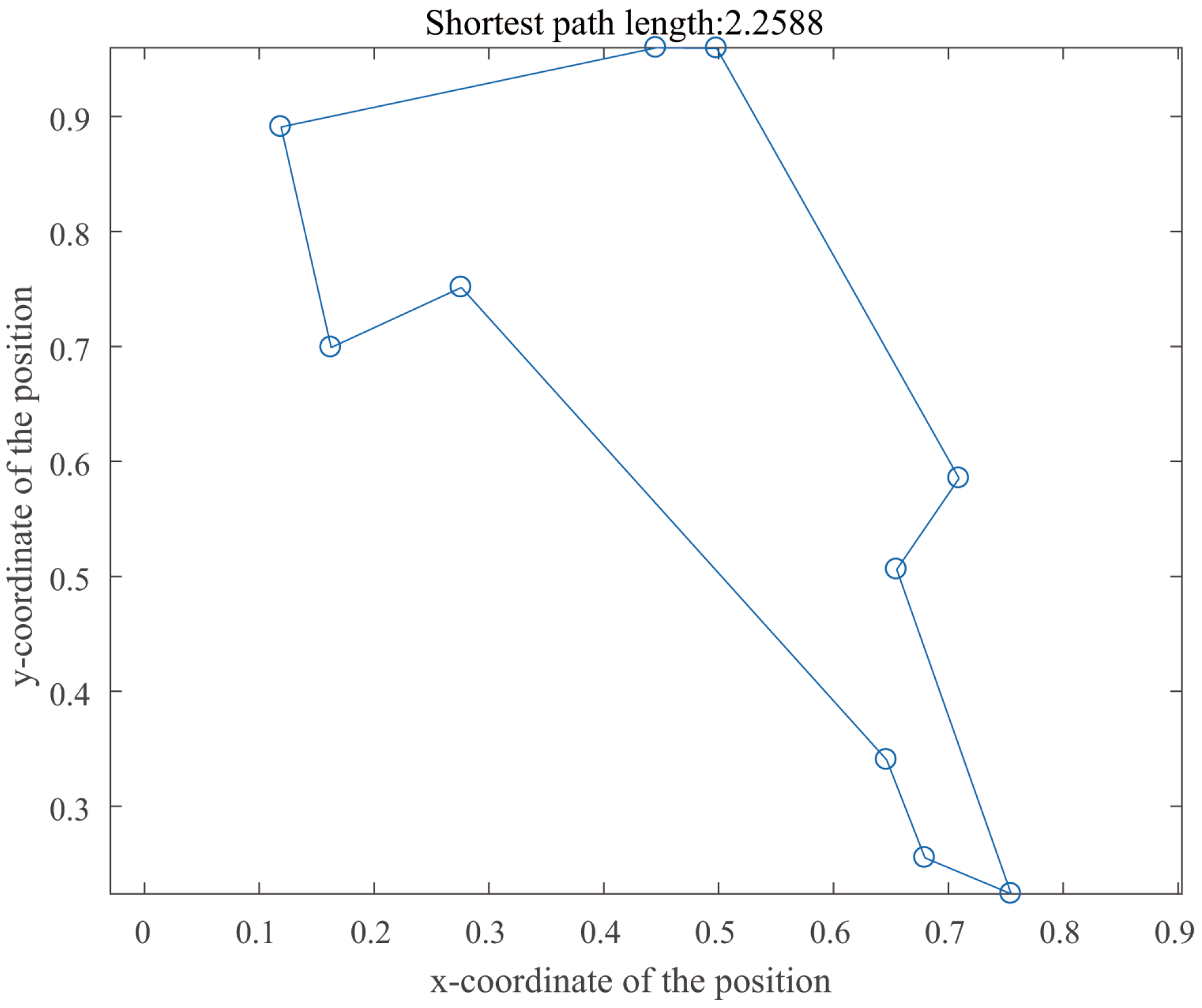
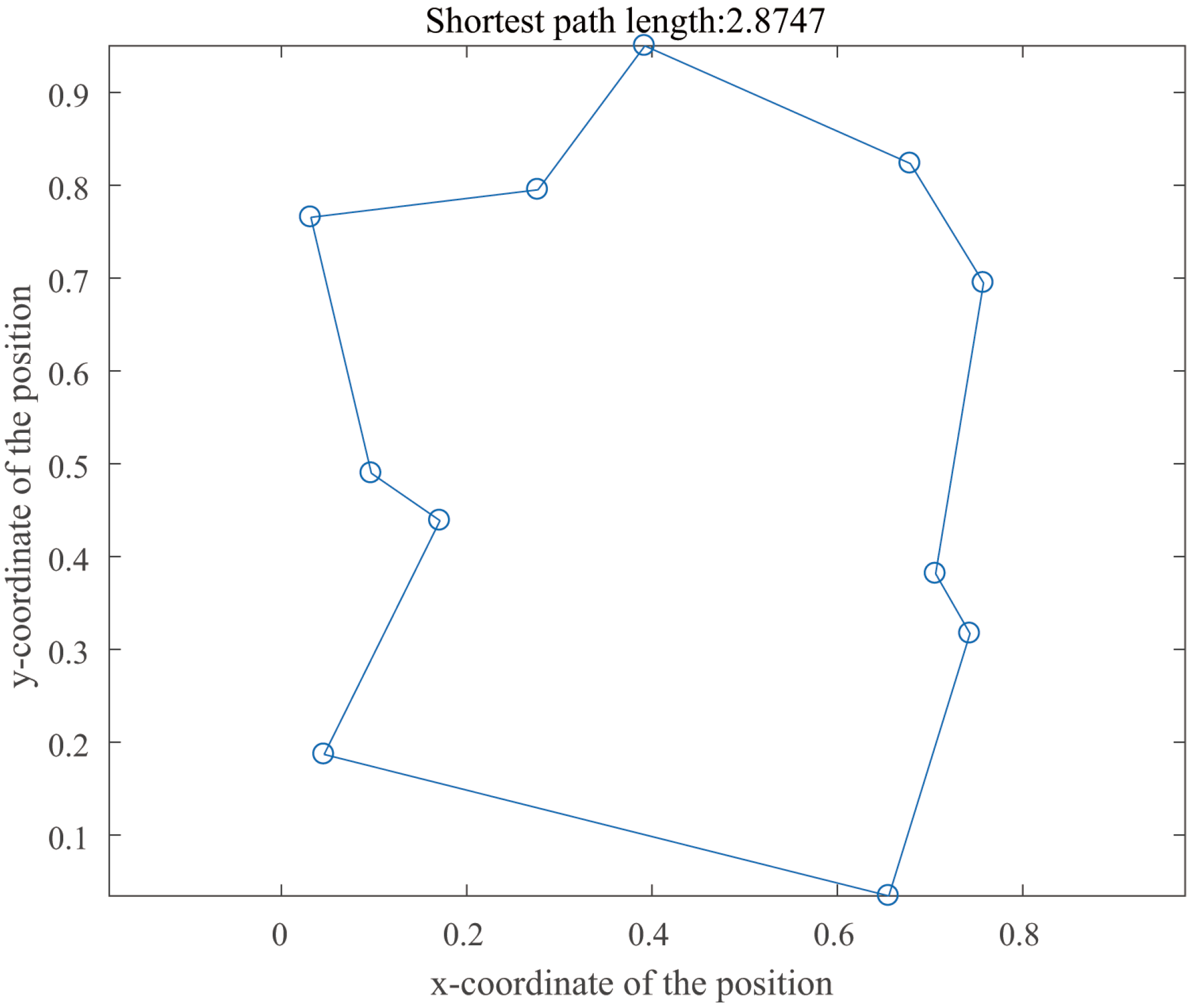
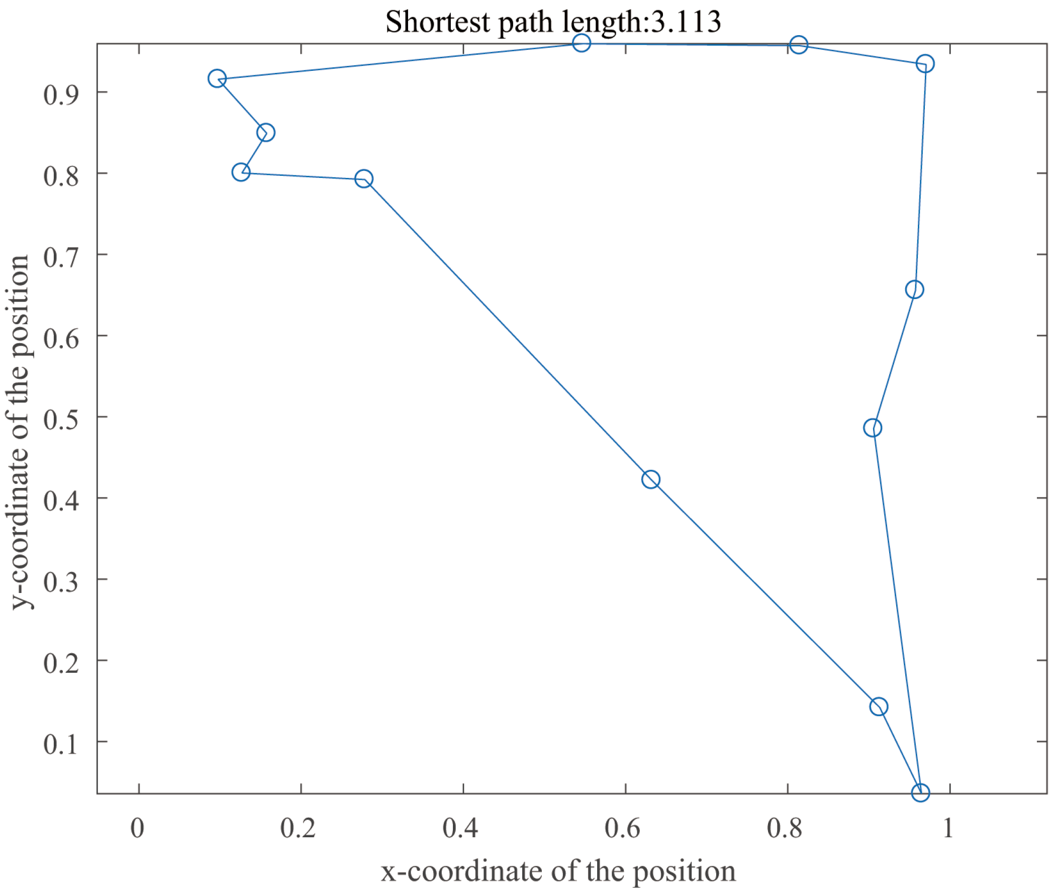
It can be seen from Figure 11, Figure 12 and Figure 13 that SNN using the adaptive learning algorithm has good search ability and fast search time in the TSP of 10 cities, 11 cities and 12 cities, so as to find the shortest path. In the face of TSP in more cities, we compared the shortest path, operation time and minimum cost of SNN using adaptive learning algorithm (SNN(A)) and SNN without adaptive learning algorithm (SNN(O)), and the comparison results are shown in

Table 1. The shortest path, operation time and minimum cost comparison results of SNN(A) and SNN(O).

	Shortest Path		Operation Time/s		Minimum Cost
Cities	SNN(A)	SNN(O)	SNN(A)	SNN(O)	SNN(A)	SNN(O)
13	3.6189	3.9345	0.18	0.11	52	57
14	3.8432	4.6348	0.55	0.24	55	59
15	4.0837	4.9123	0.74	0.42	58	61
16	4.1324	5.1619	0.89	0.65	62	69
17	4.8756	5.6537	1.15	0.77	65	73
18	5.0019	5.9871	2.68	0.81	68	78
19	5.3126	6.1566	3.15	0.89	71	85
20	5.8427	7.0234	3.22	1.08	72	89

.

As can be seen from Table 1, as the number of cities increases from 13 to 20, the operation time for both SNN(A) and SNN(O) increases. The weight update mechanism is a fundamental part of the SNN’s learning and adaptation process. The computational complexity of the weight update equation, which scales with the number of synapses and presynaptic events, can be a major factor in this increased runtime.

For larger TSPs (with more cities), the SNN needs to handle more complex path representations, which may require more neurons and synapses. This leads to a higher computational cost for the weight update step, as there are more weights to update and more presynaptic events to consider. This scalability issue means that as the problem size grows, the runtime of the SNN-based path-finding solution may increase significantly, which is a concern for real-world applications where large-scale TSP or similar path-finding problems need to be solved efficiently.

5. Conclusions

In this paper, we propose an adaptive learning algorithm based on the simplified spiking neural network model, which mainly adjusts the two key parts of the simplified model. One is the connection weight of synapses, which is represented by a combination of the “attenuation mechanism” and time, and the learning rate is used to adjust the weight change adaptively. The other is SNN’s self-organizing evolution method of dynamic threshold, which determines the amplification factor of dynamic threshold by two-dimensional Renyi entropy method and realizes self-organizing dynamic adjustment of threshold. Finally, through a series of simulation experiments, we can verify the feasibility and effectiveness of the proposed adaptive learning algorithm based on the SNN model for solving global optimization problems.

Finally, SNN is the main candidate for realizing low power intelligent computing. In the future, we will implement the SNN with the adaptive learning algorithm proposed in this paper by using Memristor (a memory resistor) in hardware, so as to better configure the SNN to overcome its inherent training limitations and achieve better application and development in target detection and multi-target recognition.

References

1. Zhu, M.; Yang, Q.; Dong, J.; Zhang, G.; Gou, X.; Rong, H.; Paul, P.; Neri, F. An adaptive optimization spiking neural P system for binary problems. Int. J. Neural Syst. 2021, 31, 2050054. [Google Scholar]
2. Woodward, A.; Froese, T.; Ikegami, T. Neural coordination can be enhanced by occasional interruption of normal firing patterns: A self-optimizing spiking neural network model. Neural Netw. 2015, 62, 39–46. [Google Scholar] [CrossRef] [PubMed]
3. Lee, W.W.; Kukreja, S.L.; Thakor, N.V. CONE: Convex-optimized-synaptic efficacies for temporally precise spike map. IEEE Trans. Neural Netw. Learn. Syst. 2016, 28, 849–861. [Google Scholar] [PubMed]
4. Zuo, L.; Chen, Y.; Zhang, L.; Chen, C. A spiking neural network with probability information transmission. Neurocomputing 2020, 408, 1–12. [Google Scholar] [CrossRef]
5. Maas, W. Noisy spiking neurons with temporal coding have more computational power than sigmoidal neurons. Adv. Neural Inf. Process. Syst. 1997, 9, 211–217. [Google Scholar]
6. Paredes-Vallés, F.; Scheper, K.Y.; De Croon, G.C. Unsupervised learning of a hierarchical spiking neural network for optical flow estimation: From events to global motion perception. IEEE Trans. Pattern Anal. Mach. Intell. 2019, 42, 2051–2064. [Google Scholar] [CrossRef]
7. Nazari, S.; Faez, K.; Janahmadi, M. A new approach to detect the coding rule of the cortical spiking model in the information transmission. Neural Netw. 2018, 99, 68–78. [Google Scholar]
8. Guo, W.; Fouda, M.E.; Yantir, H.E.; Eltawil, A.M.; Salama, K.N. Unsupervised adaptive weight pruning for energy-efficient neuromorphic systems. Front. Neurosci. 2020, 14, 598876. [Google Scholar] [CrossRef]
9. Zhang, M.; Qu, H.; Belatreche, A.; Chen, Y.; Yi, Z. A highly effective and robust membrane potential-driven supervised learning method for spiking neurons. IEEE Trans. Neural Netw. Learn. Syst. 2018, 30, 123–137. [Google Scholar] [CrossRef]
10. Guo, W.; Yantır, H.E.; Fouda, M.E.; Eltawil, A.M.; Salama, K.N. Towards efficient neuromorphic hardware: Unsupervised adaptive neuron pruning. Electronics 2020, 9, 1059. [Google Scholar] [CrossRef]
11. Jiang, H.; Zhang, H.; Xie, X.; Han, J. Neural-network-based learning algorithms for cooperative games of discrete-time multi-player systems with control constraints via adaptive dynamic programming. Neurocomputing 2019, 344, 13–19. [Google Scholar] [CrossRef]
12. Richert, D.; Masaud, K.; Macnab, C.J.B. Discrete-time weight updates in neural-adaptive control. Soft Comput. 2013, 17, 431–444. [Google Scholar] [CrossRef]
13. Shrestha, S.B.; Song, Q. Robust spike-train learning in spike-event based weight update. Neural Netw. 2017, 96, 33–46. [Google Scholar] [CrossRef] [PubMed]
14. Lim, S.; Bae, J.H.; Eum, J.H.; Lee, S.; Kim, C.H.; Kwon, D.; Park, B.G.; Lee, J.H. Adaptive learning rule for hardware-based deep neural networks using electronic synapse devices. Neural Comput. Appl. 2019, 31, 8101–8116. [Google Scholar] [CrossRef]
15. Emelyanov, A.V.; Nikiruy, K.E.; Serenko, A.V.; Sitnikov, A.V.; Presnyakov, M.Y.; Rybka, R.B.; Sboev, A.G.; Rylkov, V.V.; Kashkarov, P.K.; Kovalchuk, M.V.; et al. Self-adaptive STDP-based learning of a spiking neuron with nanocomposite memristive weights. Nanotechnology 2019, 31, 045201. [Google Scholar] [CrossRef]
16. Pilly, P.K.; Grossberg, S. Spiking neurons in a hierarchical self-organizing map model can learn to develop spatial and temporal properties of entorhinal grid cells and hippocampal place cells. PLoS ONE 2013, 8, e60599. [Google Scholar] [CrossRef]
17. Shrestha, S.B.; Song, Q. Adaptive learning rate of SpikeProp based on weight convergence analysis. Neural Netw. 2015, 63, 185–198. [Google Scholar] [CrossRef]
18. Bodyanskiy, Y.; Dolotov, A.; Vynokurova, O. Evolving spiking wavelet-neuro-fuzzy self-learning system. Appl. Soft Comput. 2014, 14, 252–258. [Google Scholar] [CrossRef]
19. RamachandranPillai, R.; Arock, M. An adaptive spiking neural P system for solving vehicle routing problems. Arab. J. Sci. Eng. 2020, 45, 2513–2529. [Google Scholar] [CrossRef]
20. Howard, D.; Bull, L.; de Lacy Costello, B. Evolving unipolar memristor spiking neural networks. Connect. Sci. 2015, 27, 397–416. [Google Scholar] [CrossRef]
21. Salt, L.; Howard, D.; Indiveri, G.; Sandamirskaya, Y. Parameter optimization and learning in a spiking neural network for UAV obstacle avoidance targeting neuromorphic processors. IEEE Trans. Neural Netw. Learn. Syst. 2019, 31, 3305–3318. [Google Scholar] [CrossRef]
22. Wang, J.; Belatreche, A.; Maguire, L.P.; McGinnity, T.M. Spiketemp: An enhanced rank-order-based learning approach for spiking neural networks with adaptive structure. IEEE Trans. Neural Netw. Learn. Syst. 2015, 28, 30–43. [Google Scholar] [CrossRef] [PubMed]
23. Maass, W. Networks of spiking neurons: The third generation of neural network models. Neural Netw. 1997, 10, 1659–1671. [Google Scholar] [CrossRef]
24. Salazar-Varas, R.; Vazquez, R.A. Evaluating spiking neural models in the classification of motor imagery EEG signals using short calibration sessions. Appl. Soft Comput. 2018, 67, 232–244. [Google Scholar] [CrossRef]
25. Wang, X.; Lin, X.; Dang, X. Supervised learning in spiking neural networks: A review of algorithms and evaluations. Neural Netw. 2020, 125, 258–280. [Google Scholar] [CrossRef]
26. Strohmer, B.; Stagsted, R.K.; Manoonpong, P.; Larsen, L.B. Integrating non-spiking interneurons in spiking neural networks. Front. Neurosci. 2021, 15, 633945. [Google Scholar] [CrossRef]
27. Zhang, Z.; Liu, Q. Spike-event-driven deep spiking neural network with temporal encoding. IEEE Signal Process. Lett. 2021, 28, 484–488. [Google Scholar]
28. Markov, S.; Kyurkchiev, N.; Iliev, A.; Rahnev, A. On the approximation of the generalized cut functions of degree p + 1 by smooth hyper-log-logistic function. Dyn. Syst. Appl. 2018, 27, 715–728. [Google Scholar]
29. Yin, Y. Random neural network methods and deep learning. Probab. Eng. Informational Sci. 2021, 35, 6–36. [Google Scholar]
30. Basanisi, R.; Brovelli, A.; Cartoni, E.; Baldassarre, G. A generative spiking neural-network model of goal-directed behaviour and one-step planning. PLoS Comput. Biol. 2020, 16, e1007579. [Google Scholar] [CrossRef]
31. Kim, J.; Kim, H.; Huh, S.; Lee, J.; Choi, K. Deep neural networks with weighted spikes. Neurocomputing 2018, 311, 373–386. [Google Scholar] [CrossRef]
32. Panda, P.; Allred, J.M.; Ramanathan, S.; Roy, K. Asp: Learning to forget with adaptive synaptic plasticity in spiking neural networks. IEEE J. Emerg. Sel. Top. Circuits Syst. 2017, 8, 51–64. [Google Scholar] [CrossRef]
33. Panda, P.; Aketi, S.A.; Roy, K. Toward scalable, efficient, and accurate deep spiking neural networks with backward residual connections, stochastic softmax, and hybridization. Front. Neurosci. 2020, 14, 535502. [Google Scholar] [CrossRef] [PubMed]
34. Huang, X.; Zheng, Z.; Hu, G.; Wu, S.; Rasch, M.J. Different propagation speeds of recalled sequences in plastic spiking neural networks. New J. Phys. 2015, 17, 035006. [Google Scholar] [CrossRef]
35. Lobov, S.A.; Mikhaylov, A.N.; Shamshin, M.; Makarov, V.A.; Kazantsev, V.B. Spatial properties of STDP in a self-learning spiking neural network enable controlling a mobile robot. Front. Neurosci. 2020, 14, 491341. [Google Scholar] [CrossRef]
36. Buesing, L.; Bill, J.; Nessler, B.; Maass, W. Neural dynamics as sampling: A model for stochastic computation in recurrent networks of spiking neurons. PLoS Comput. Biol. 2011, 7, e1002211. [Google Scholar] [CrossRef]
37. Krunglevicius, D. Competitive STDP learning of overlapping spatial patterns. Neural Comput. 2015, 27, 1673–1685. [Google Scholar] [CrossRef]
38. Peng, Y.; Wu, J.; Zou, L.; Feng, Y.; Tu, Z. A generalization of the cauchy-schwarz inequality and its application to stability analysis of nonlinear impulsive control systems. Complexity 2019, 2019, 6048909. [Google Scholar]
39. Demin, V.A.; Nekhaev, D.V.; Surazhevsky, I.A.; Nikiruy, K.E.; Emelyanov, A.V.; Nikolaev, S.N.; Rylkov, V.V.; Kovalchuk, M.V. Necessary conditions for STDP-based pattern recognition learning in a memristive spiking neural network. Neural Netw. 2021, 134, 64–75. [Google Scholar] [CrossRef]
40. Hao, Y.; Huang, X.; Dong, M.; Xu, B. A biologically plausible supervised learning method for spiking neural networks using the symmetric STDP rule. Neural Netw. 2020, 121, 387–395. [Google Scholar]
41. Rathi, N.; Panda, P.; Roy, K. STDP-based pruning of connections and weight quantization in spiking neural networks for energy-efficient recognition. IEEE Trans. Comput.-Aided Des. Integr. Circuits Syst. 2018, 38, 668–677. [Google Scholar] [CrossRef]
42. Strain, T.J.; McDaid, L.J.; McGinnity, T.M.; Maguire, L.P.; Sayers, H.M. An STDP training algorithm for a spiking neural network with dynamic threshold neurons. Int. J. Neural Syst. 2010, 20, 463–480. [Google Scholar] [CrossRef]
43. Nasser, H.; Cessac, B. Parameter estimation for spatio-temporal maximum entropy distributions: Application to neural spike trains. Entropy 2014, 16, 2244–2277. [Google Scholar] [CrossRef]
44. Wang, Z.; Davis, E.J. Calculating Rényi entropies with neural autoregressive quantum states. Phys. Rev. A 2020, 102, 062413. [Google Scholar] [CrossRef]
45. Bashkirov, A.G.E. Renyi entropy as a statistical entropy for complex systems. Theor. Math. Phys. 2006, 149, 1559–1573. [Google Scholar] [CrossRef]
46. Bickel, D.R. Model averages sharpened into Occam’s razors: Deep learning enhanced by Rényi entropy. Commun. Stat.-Theory Methods 2022, 51, 8283–8295. [Google Scholar] [CrossRef]
47. Salah Eddine, M.; El Joumani, S.; Zennouhi, R.; Masmoudi, L. Multi-objective optimization for worldview image segmentation funded on the entropies of tsallis and rényi. Multimed. Tools Appl. 2020, 79, 30637–30652. [Google Scholar]
48. Shamsaldin, A.S.; Rashid, T.A.; Al-Rashid Agha, R.A.; Al-Salihi, N.K.; Mohammadi, M. Donkey and smuggler optimization algorithm: A collaborative working approach to path finding. J. Comput. Des. Eng. 2019, 6, 562–583. [Google Scholar] [CrossRef]
Figure 1. The structure model of a single spiking neuron.
Symmetry 17 01814 g001
Figure 2. Changes in average synaptic weight of SNN without the adaptive learning algorithm.
Symmetry 17 01814 g002
Figure 3. Dynamic threshold changes in SNN without the adaptive learning algorithm.
Symmetry 17 01814 g003
Figure 4. Changes in average synaptic weight of SNN with the adaptive learning algorithm.
Symmetry 17 01814 g004
Figure 5. Dynamic threshold changes in SNN with the adaptive learning algorithm.
Symmetry 17 01814 g005
Figure 6. Changes in the average synaptic weight in 1000 neurons.
Symmetry 17 01814 g006
Figure 7. Dynamic threshold changes in 1000 neurons.
Symmetry 17 01814 g007
Figure 8. Changes in average synaptic weight of different stimulus spikes.
Symmetry 17 01814 g008
Figure 9. Dynamic threshold changes in different stimulus spikes.
Symmetry 17 01814 g009
Figure 10. Comparison of the convergence rate of the algorithm with different ρ and μ .
Symmetry 17 01814 g010
Figure 11. SNN with adaptive learning algorithm is applied to TSP in 10 cities.
Symmetry 17 01814 g011
Figure 12. SNN with adaptive learning algorithm is applied to TSP in 11 cities.
Symmetry 17 01814 g012
Figure 13. SNN with adaptive learning algorithm is applied to TSP in 12 cities.
Symmetry 17 01814 g013