Bias Term for Outlier Detection and Robust Regression

Abstract

Noisy data and outliers are among the main challenges in machine learning, as their presence in training data can significantly reduce model performance and generalization. Detecting and handling these anomalous samples is particularly difficult because it is hard to distinguish them from normal data. In this study, we propose a novel bias-based method (BT-SVR) to detect outliers and noisy inputs. The method uses a bias term derived from pairwise relationships among data points, which captures structural information about input distances. Outliers and noisy samples typically produce near-zero bias responses, allowing them to be identified effectively. A root-mean-square (RMS) scoring mechanism is then applied to quantify the anomaly strength of each sample, enabling the impact of outliers to be underweighted before training. Experiments demonstrate that BT-SVR improves the performance of Support Vector Regression (SVR) and enhances its robustness against noisy and anomalous data.

1. Introduction

In machine learning, the quality of training data is crucial for building robust and generalizable models. However, real-world datasets often contain noisy data and outliers, which can degrade model performance by introducing errors and reducing predictive accuracy [1]. Noisy data, marked by random errors and outliers, defined as points that deviate significantly from the norm, pose challenges because they are hard to distinguish from valid samples [2]. These deviations can lead to overfitting or poor generalization, especially in regression and classification tasks [1]. As machine-learning applications grow in critical areas like healthcare [3], finance [4], and autonomous systems [5], the need to detect and mitigate noisy data and outliers has become increasingly urgent [6].

Regression, a core machine-learning task, aims to model relationships between input vectors and known outputs [7]. However, noisy data and outliers disrupt these relationships, reducing the robustness of regression algorithms and their ability to perform well [7]. Existing methods to handle these issues fall into three categories: preprocessing techniques [8] that filter anomalies, sample polishing techniques [9] that correct corrupted data, and robust training algorithms [10,11,12,13,14,15]. Preprocessing struggles to differentiate noisy samples from valid ones, while polishing is time-consuming and often limited to small datasets [16]. Robust training algorithms, such as those based on Support Vector Regression (SVR)—an extension of Support Vector Machines (SVM) [17], offer promising solutions but still face challenges in high-dimensional or context-dependent datasets where anomalies are subtle.

Traditional outlier-detection methods, like statistical thresholding or distance-based approaches, often fail to capture structural relationships among data points, limiting their effectiveness in complex datasets [2]. To address this, we propose a novel bias-based method, BT-SVR, for detecting outliers and noisy inputs. This method uses a bias term derived from pairwise data relationships to capture structural information about input distances. Outliers and noisy samples typically produce near-zero bias responses, enabling their identification. We then apply a root-mean-square (RMS) scoring mechanism to quantify anomaly strength, allowing the impact of outliers to be reduced before training. Our experiments show that BT-SVR enhances SVR performance and robustness against noisy and anomalous data.

The main contributions of this paper are:

• Introduces a novel bias-based outlier detection method using a bias term derived from pairwise input relationships of the RBF kernel.
• Improves SVR robustness by underweighting outliers identified via RMS scoring of the bias values.

2. Derivation of the Bias Term

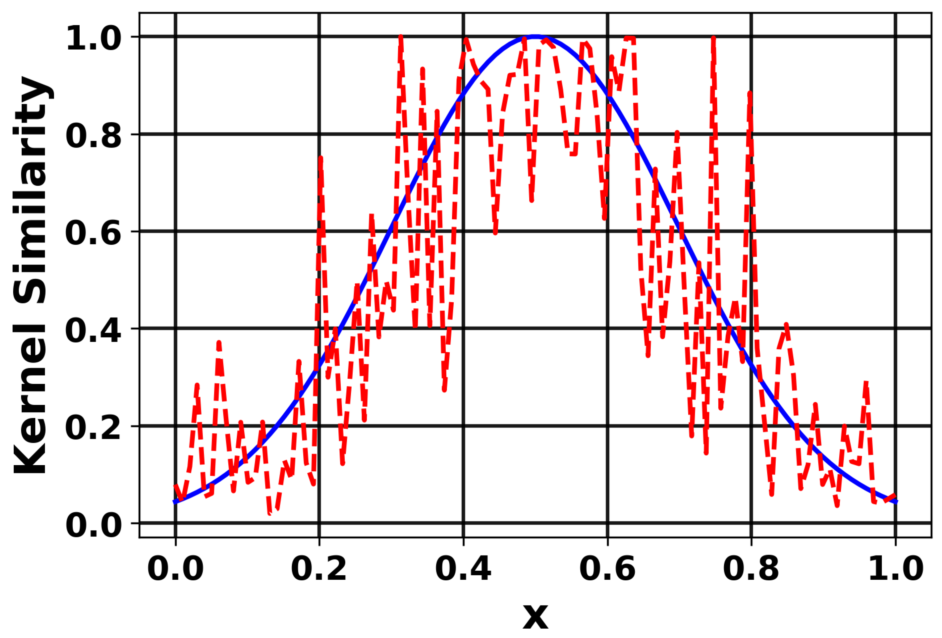
In this section, we derive the bias introduced by additive noise in the Gaussian Radial Basis Function (RBF) kernel when both inputs are noisy, as illustrated in Figure 1. The plot illustrates the effect of noise on kernel similarity when using the RBF kernel. The blue solid line represents the original clean input signal, while the red dashed line shows the same input after being corrupted by noise. As observed, the presence of noise distorts the input pattern, thereby reducing the similarity values computed by the RBF kernel. This demonstrates the sensitivity of the RBF kernel to noise in the input data.

Let the observed noisy inputs be $\tilde{u}=u+\eta \in {\mathbb{R}}^d$ and $\tilde{v}=v+\xi \in {\mathbb{R}}^d$, where u and v are the clean inputs. The noise vectors $\eta$ and $\xi$ are assumed to be independent, zero-mean, isotropic, with covariance ${\mathrm{\Sigma }}_{\eta }={\mathrm{\Sigma }}_{\xi }={\sigma }_{\eta }^2{I}_d$.

The Gaussian RBF kernel is defined as:

$$K(\tilde{u},\tilde{v})=exp\left(-{\displaystyle \frac{\parallel \tilde{u}-\tilde{v}{\parallel }^2}{2{\sigma }^2}}\right),$$

(1)

where $\sigma$ is the kernel bandwidth. We introduce additional independent noises ${\eta }^{\prime }$ and ${\xi }^{\prime }$ with the same distribution, and aim to approximate the bias term introduced into the kernel using a second-order Taylor series expansion [18] centered on the clean inputs. Expanding the kernel function around the noisy inputs $\tilde{u}$ and $\tilde{v}$ using a second-order Taylor approximation gives:

$$\begin{array}{cc}\hfill K(\tilde{u}+{\eta }^{\prime },\tilde{v}+{\xi }^{\prime })\approx & K(\tilde{u},\tilde{v})+{\nabla }_{\tilde{u}}{K}^{\top }{\eta }^{\prime }+{\nabla }_{\tilde{v}}{K}^{\top }{\xi }^{\prime }\hfill \\ \hfill & +{\displaystyle \frac{1}{2}}{\left({\eta }^{\prime }\right)}^{\top }{H}_{\tilde{u}}{\eta }^{\prime }+{\left({\eta }^{\prime }\right)}^{\top }{H}_{\tilde{u}\tilde{v}}{\xi }^{\prime }\hfill \\ \hfill & +{\displaystyle \frac{1}{2}}{\left({\xi }^{\prime }\right)}^{\top }{H}_{\tilde{v}}{\xi }^{\prime }.\hfill \end{array}$$

(2)

where ${\nabla }_{\tilde{u}}K$ and ${\nabla }_{\tilde{v}}K$ are the gradients, and $H_{\tilde{u}}$, $H_{\tilde{v}}$, $H_{\tilde{u}\tilde{v}}$ are the Hessians [19] of the kernel with respect to $\tilde{u}$, $\tilde{v}$, and mixed derivatives, respectively. Higher-order terms are neglected here.

Taking the expectation over the noises ${\eta }^{\prime }$ and ${\xi }^{\prime }$, and using $\mathbb{E}\left[{\eta }^{\prime }\right]=\mathbb{E}\left[{\xi }^{\prime }\right]=0$, the linear and mixed terms in the Taylor expansion of Equation (2) vanish. Consequently, the expected kernel value can be approximated as

$$\mathbb{E}\left[K(\tilde{u}+{\eta }^{\prime },\tilde{v}+{\xi }^{\prime })\right]\approx K(\tilde{u},\tilde{v})+{\displaystyle \frac{1}{2}}Tr\left(H_{\tilde{u}}{\mathrm{\Sigma }}_{{\eta }^{\prime }}\right)+{\displaystyle \frac{1}{2}}Tr\left(H_{\tilde{v}}{\mathrm{\Sigma }}_{{\xi }^{\prime }}\right),$$

(3)

where the remaining terms involve only the Hessians [19] and the noise covariances. From Equation (2), we need to derive the gradient of the RBF kernel.

Define $\delta =\tilde{u}-\tilde{v}$ and $\gamma ={\displaystyle \frac{1}{2{\sigma }^2}}$, so $K(\tilde{u},\tilde{v})={exp(-\gamma \parallel \delta \parallel }^2)$.

The gradient with respect to $\tilde{u}$ is

$${\nabla }_{\tilde{u}}K(\tilde{u},\tilde{v})={\displaystyle \frac{\partial }{\partial \tilde{u}}}exp\left(-\gamma \sum _{k=1}^d{({\tilde{u}}_k-{\tilde{v}}_k)}^2\right)=-2\gamma K(\tilde{u},\tilde{v})\delta .$$

(4)

By symmetry of the Gaussian kernel, the gradient with respect to $\tilde{v}$ can be obtained as

$${\nabla }_{\tilde{v}}K(\tilde{u},\tilde{v})=-{\nabla }_{\tilde{u}}K(\tilde{u},\tilde{v})=2\gamma K(\tilde{u},\tilde{v})\delta .$$

(5)

The Hessian with respect to $\tilde{u}$ is the matrix of second derivatives, obtained by differentiating the gradient

$${\nabla }_{\tilde{u}}K(\tilde{u},\tilde{v})=-2\gamma K(\tilde{u},\tilde{v})(\tilde{u}-\tilde{v}).$$

(6)

For the i-th component of $\tilde{u}$:

$${\displaystyle \frac{\partial K}{\partial {\tilde{u}}_i}}=-2\gamma K(\tilde{u},\tilde{v})({\tilde{u}}_i-{\tilde{v}}_i).$$

(7)

The $(i,j)$-th element of the Hessian is:

$$\begin{array}{cc}\hfill {\left(H_{\tilde{u}}\right)}_{ij}& ={\displaystyle \frac{\partial }{\partial {\tilde{u}}_j}}\left[-2\gamma K(\tilde{u},\tilde{v})({\tilde{u}}_i-{\tilde{v}}_i)\right]\hfill \\ \hfill & =-2\gamma \left[-2\gamma K(\tilde{u},\tilde{v})({\tilde{u}}_i-{\tilde{v}}_i)({\tilde{u}}_j-{\tilde{v}}_j)-{\delta }_{ij}K(\tilde{u},\tilde{v})\right].\hfill \end{array}$$

(8)

where ${\delta }_{ij}$ is the Kronecker delta. Then

$$H_{\tilde{u}}(\tilde{u},\tilde{v})=2\gamma K(\tilde{u},\tilde{v})(2\gamma \delta {\delta }^T-I_d).$$

By symmetry, $H_{\tilde{v}}(\tilde{u},\tilde{v})=2\gamma K(\tilde{u},\tilde{v})(2\gamma \delta {\delta }^T-I_d)$.

From Equation (2), we also need to compute the Trace [19].

For isotropic noise, the covariance matrix of the noise is a scaled identity, ${\mathrm{\Sigma }}_{{\eta }^{\prime }}={\sigma }_{\eta }^2{I}_d$, so the trace term becomes:

$$\mathrm{Tr}\left(H_{\tilde{u}}{\mathrm{\Sigma }}_{{\eta }^{\prime }}\right)={\sigma }_{\eta }^2\mathrm{Tr}\left(H_{\tilde{u}}\right).$$

(9)

Next, we compute the trace of the Hessian explicitly:

$$\begin{array}{cc}\hfill \mathrm{Tr}\left(H_{\tilde{u}}\right)& =\mathrm{Tr}\left(2\gamma K(\tilde{u},\tilde{v})(2\gamma \delta {\delta }^{\top }-I_d)\right)\hfill \\ \hfill & =2\gamma K(\tilde{u},\tilde{v})\left({2\gamma \parallel \delta \parallel }^2-d\right),\hfill \end{array}$$

(10)

Since $\gamma ={\displaystyle \frac{1}{2{\sigma }^2}}$, we have $2\gamma ={\displaystyle \frac{1}{{\sigma }^2}}$, $4{\gamma }^2={\displaystyle \frac{1}{{\sigma }^4}}$, and ${\parallel \delta \parallel }^2={\parallel \tilde{u}-\tilde{v}\parallel }^2$. Then:

$$\begin{array}{cc}\hfill \mathrm{Tr}\left(H_{\tilde{u}}(\tilde{u},\tilde{v})\right)& ={\displaystyle \frac{1}{{\sigma }^2}}K(\tilde{u},\tilde{v})\left({\displaystyle \frac{\parallel \tilde{u}-\tilde{v}{\parallel }^2}{{\sigma }^2}}-d\right)\hfill \\ \hfill & =K(\tilde{u},\tilde{v})\left({\displaystyle \frac{\parallel \tilde{u}-\tilde{v}{\parallel }^2}{{\sigma }^4}}-{\displaystyle \frac{d}{{\sigma }^2}}\right).\hfill \end{array}$$

(11)

Recall in Equation (2) that

$$\begin{array}{cc}\hfill \mathrm{E}\left[K(\tilde{u}+{\eta }^{\prime },\tilde{v}+{\xi }^{\prime })\right]-K(\tilde{u},\tilde{v})& \approx {\displaystyle \frac{1}{2}}\mathrm{Tr}\left(H_{\tilde{u}}(\tilde{u},\tilde{v}){\mathrm{\Sigma }}_{{\eta }^{\prime }}\right)+{\displaystyle \frac{1}{2}}\mathrm{Tr}\left(H_{\tilde{v}}(\tilde{u},\tilde{v}){\mathrm{\Sigma }}_{{\xi }^{\prime }}\right)\hfill \\ \hfill & ={\sigma }_{\eta }^{2}K(\tilde{u},\tilde{v})\left({\displaystyle \frac{\parallel \tilde{u}-\tilde{v}{\parallel }^2}{{\sigma }^4}}-{\displaystyle \frac{d}{{\sigma }^2}}\right).\hfill \end{array}$$

(12)

The Bias term is

$${\sigma }_{\eta }^{2}K(\tilde{u},\tilde{v})\left({\displaystyle \frac{\parallel \tilde{u}-\tilde{v}{\parallel }^2}{{\sigma }^4}}-{\displaystyle \frac{d}{{\sigma }^2}}\right).$$

(13)

3. Proposed Method

This study proposes a novel outlier detection method, BT-SVR, which uses the bias term induced by additive noise in the Gaussian Radial Basis Function (RBF) kernel. This method is based on a second-order Taylor expansion and takes advantage of the kernel’s sensitivity to Euclidean distances between data points, enabling the identification of outliers.

3.1. Utilization of Kernel Mathematical Properties for Outlier Detection

The outlier detection method exploits the asymptotic behavior of the bias term as the Euclidean distance between data points increases, a property inherent to the Gaussian RBF kernel. The kernel is defined as $K(\tilde{u},\tilde{v})=exp\left(-{\displaystyle \frac{\parallel \tilde{u}-\tilde{v}{\parallel }^2}{2{\sigma }^2}}\right)$, where $\tilde{u}=u+\eta$ and $\tilde{v}=v+\xi$ are noisy observations with noise vectors $\eta$ and $\xi$ having covariance ${\mathrm{\Sigma }}_{\eta }={\mathrm{\Sigma }}_{\xi }={\sigma }_{\eta }^2{I}_d$. A second-order Taylor expansion around the noisy inputs, followed by expectation over additional independent noise ${\eta }^{\prime }$ and ${\xi }^{\prime }$, yields the bias approximation:

$$\mathbb{E}\left[K(\tilde{u}+{\eta }^{\prime },\tilde{v}+{\xi }^{\prime })\right]-K(\tilde{u},\tilde{v})\approx {\sigma }_{\eta }^{2}K(\tilde{u},\tilde{v})\left({\displaystyle \frac{\parallel \tilde{u}-\tilde{v}{\parallel }^2}{{\sigma }^4}}-{\displaystyle \frac{d}{{\sigma }^2}}\right),$$

(14)

where ${\sigma }_{\eta }^2$ is the noise variance, $\sigma$ is the kernel bandwidth, d is the dimensionality, and $K(\tilde{u},\tilde{v})$ is the kernel evaluated at the noisy inputs. The bias term is computed for all pairs $(i,j)$ in the bias matrix as:

$$\mathrm{bias}\_\mathrm{matrix}(i,j)={\sigma }_{\eta }^{2}K(\tilde{u},\tilde{v})(i,j)\left({\displaystyle \frac{{\parallel \delta \parallel }^2}{{\sigma }^4}}-{\displaystyle \frac{d}{{\sigma }^2}}\right),$$

(15)

with $K(\tilde{u},\tilde{v})(i,j)={exp(-\gamma \parallel \delta \parallel }^2)$, $\gamma ={\displaystyle \frac{1}{2{\sigma }^2}}$, and ${\parallel \delta \parallel }^2={\parallel {\tilde{u}}_i-{\tilde{v}}_j\parallel }^2$.

The key mathematical property exploited is the kernel’s exponential decay. As ${\parallel \delta \parallel }^2\to \infty$, ${lim}_{{\parallel \delta \parallel }^2\to \infty }K(\tilde{u},\tilde{v})\to 0$ exponentially, causing $\mathrm{bias}\_\mathrm{matrix}(i,j)$ to approach zero regardless of the magnitude of ${\displaystyle \frac{{\parallel \delta \parallel }^2}{{\sigma }^4}}-{\displaystyle \frac{d}{{\sigma }^2}}$. For a fixed $\sigma$ and d, the term ${\displaystyle \frac{{\parallel \delta \parallel }^2}{{\sigma }^4}}-{\displaystyle \frac{d}{{\sigma }^2}}$ grows linearly with ${\parallel \delta \parallel }^2$, but this growth is overwhelmed by the kernel’s decay when ${\parallel \delta \parallel }^2$ exceeds a critical threshold. With $\sigma =1$ and $d=3$, the threshold occurs around ${\parallel \delta \parallel }^2\approx 3$ (i.e., $\parallel \delta \parallel \approx \sqrt{3}\approx 1.7$), where the bias transitions from non-zero (negative for ${\parallel \delta \parallel }^2<3$) to near-zero for larger distances. This behavior holds because the Gaussian kernel acts as a proximity weighting function, suppressing the bias contribution for distant pairs.

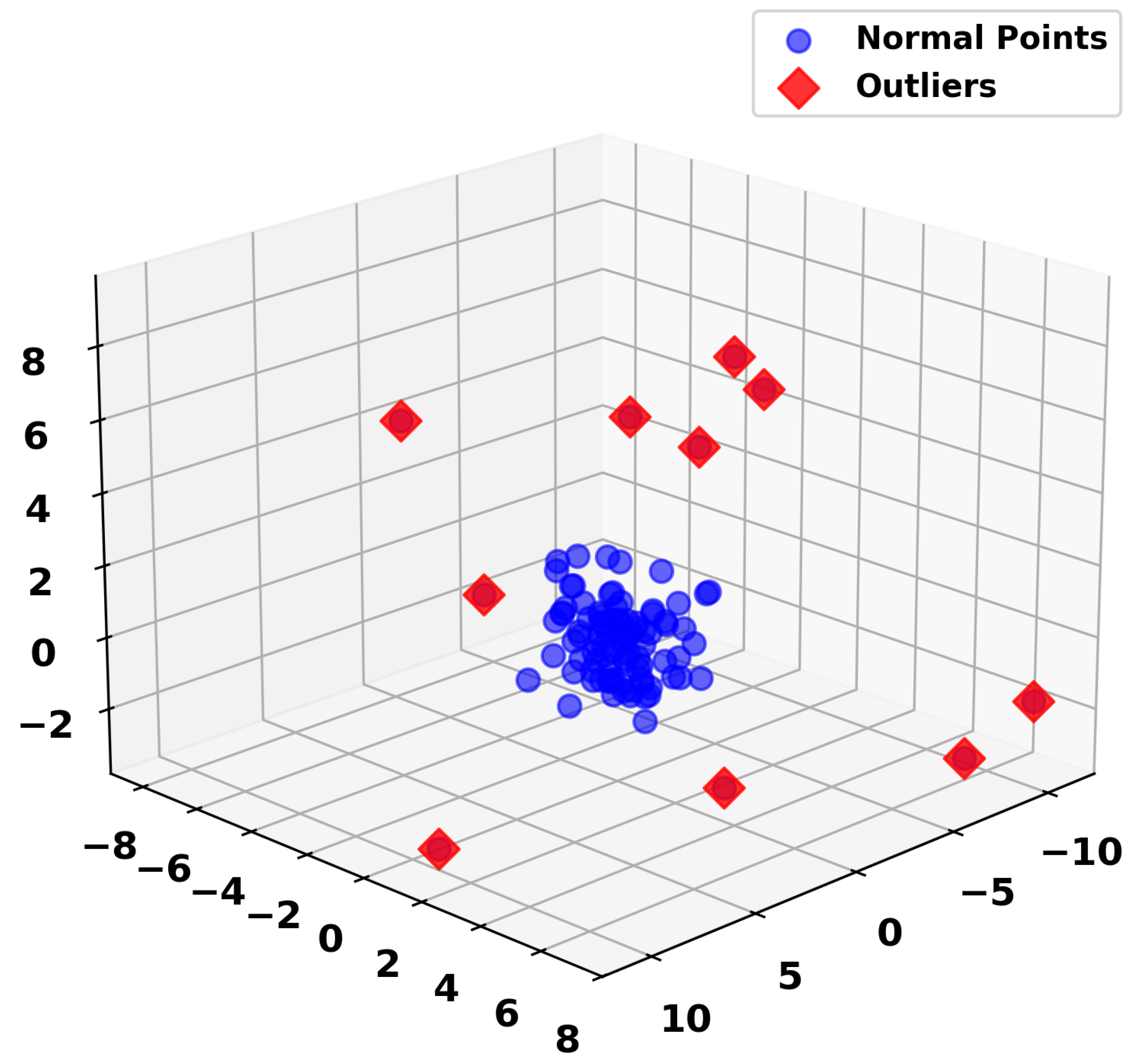
Outliers, characterized by large deviations from the bulk of the data, typically form pairs with ${\parallel \delta \parallel }^2$ well above this threshold when compared to normal points. Consequently, their corresponding $\mathrm{bias}\_\mathrm{matrix}(i,j)$ values are near zero, providing a discriminative signal. The method detects outliers by analyzing the bias matrix, hypothesizing that points involved in predominantly near-zero bias pairs are likely outliers. This property is validated by observing that the synthetic outliers, randomly selected with points scaled by a factor of 5 (see Figure 2), consistently produce near-zero bias values for points at large distances $\parallel \delta \parallel$, aligning with the bias term’s diminishing effect on outliers.

To empirically validate the hypothesis that the bias term effectively detects outliers, a synthetic dataset comprising 100 points was generated from a standard normal distribution in a 3-dimensional space. Outliers were introduced at indices 10, 20, 30, 40, 50, 60, 70, 80, 90, and 100 by applying a scaling factor of 5 to random perturbations see Figure 2, amplifying their deviation from the norm. 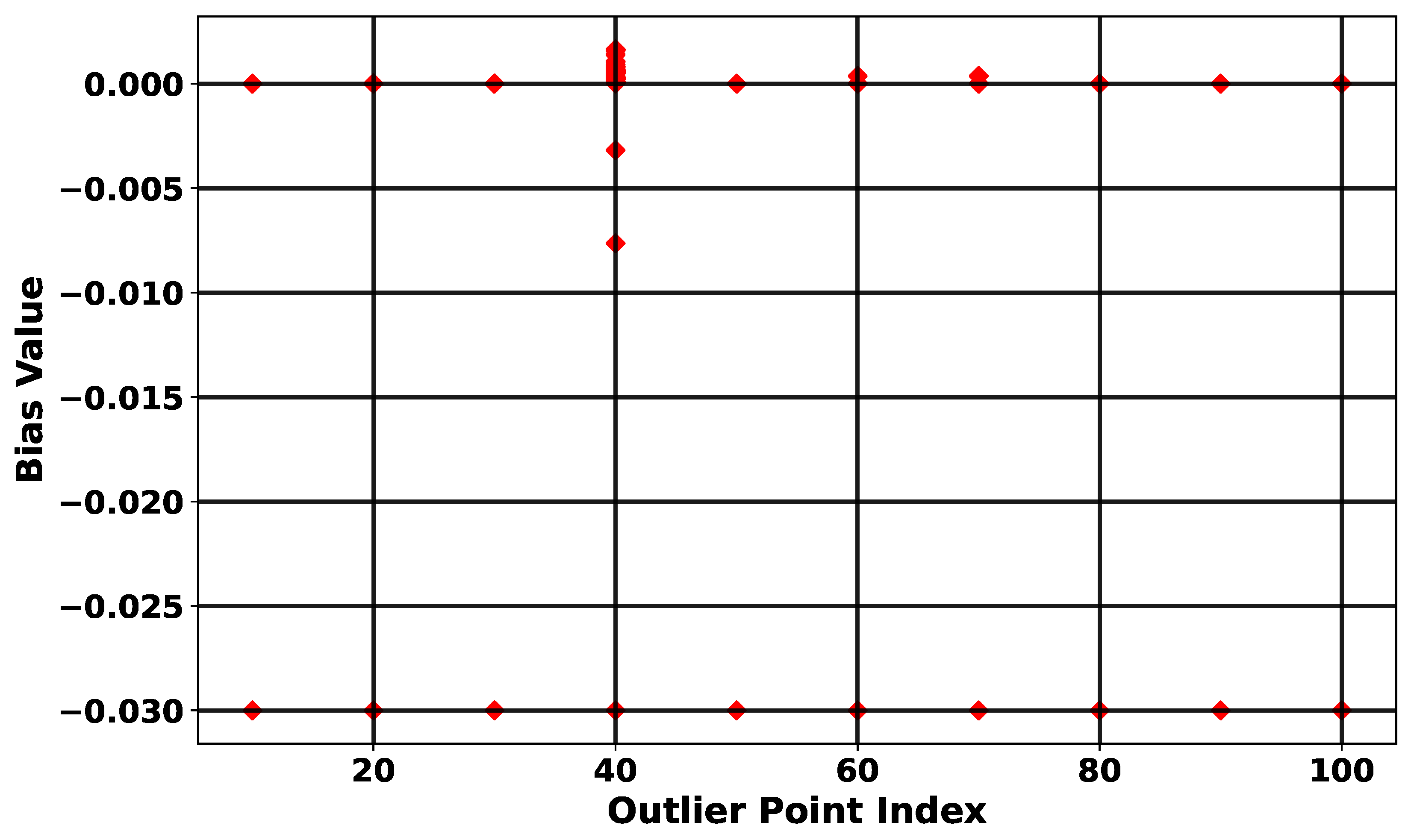Analysis of the resulting bias matrix, computed as $\mathrm{bias}\_\mathrm{matrix}(i,j)={\sigma }_{\eta }^{2}K(\tilde{u},\tilde{v})(i,j)\left({\displaystyle \frac{{\parallel \delta \parallel }^2}{{\sigma }^4}}-{\displaystyle \frac{d}{{\sigma }^2}}\right)$ with $K(\tilde{u},\tilde{v})(i,j)={exp(-\gamma \parallel \delta \parallel }^2)$ and $\gamma ={\displaystyle \frac{1}{2{\sigma }^2}}$, revealed distinct patterns. Specifically, bias values for self-pairs of outliers (where ${\parallel \delta \parallel }^2=0$) exhibited a negative peak of approximately −0.03, as shown in Figure 3. The red diamonds in Figure 3 indicate the bias values corresponding to both outliers and inliers. As shown, outliers produce near-zero bias values while inliers exhibit higher bias magnitudes, visually highlighting the differential behavior of the bias term and its ability to identify outliers effectively, reflecting the Gaussian kernel’s maximum weighting at zero Euclidean distance. Conversely, bias values for pairs involving outliers and other points, where ${\parallel \delta \parallel }^2$ is significantly increased due to the perturbations, approached near zero, supporting the exponential decay of $K(\tilde{u},\tilde{v})$.

This differential behavior highlights the kernel’s capacity to prioritize close proximity while suppressing contributions from distant pairs, thereby providing a robust foundation for outlier detection based on the weakening effect of bias values.

3.2. Root-Mean-Square (RMS) Score for Outlier Identification

To enhance the outlier detection process, the Root Mean Square (RMS) score is used to aggregate the bias values for each point, providing a quantitative criterion for outlier identification. For each point i, the RMS score is defined as:

$$\mathrm{RMS}\left(i\right)=\sqrt{{\displaystyle \frac{1}{N}}{\sum }_{j=1}^N{\left(\mathrm{bias} \mathrm{matrix}(i,j)\right)}^2},$$

(16)

where N is the total number of points, and $\mathrm{bias} \mathrm{matrix}(i,j)$ represents the bias value computed between the points i and j. This formulation captures the overall magnitude of the bias interactions, with squaring ensuring that both positive and negative contributions are accounted for.

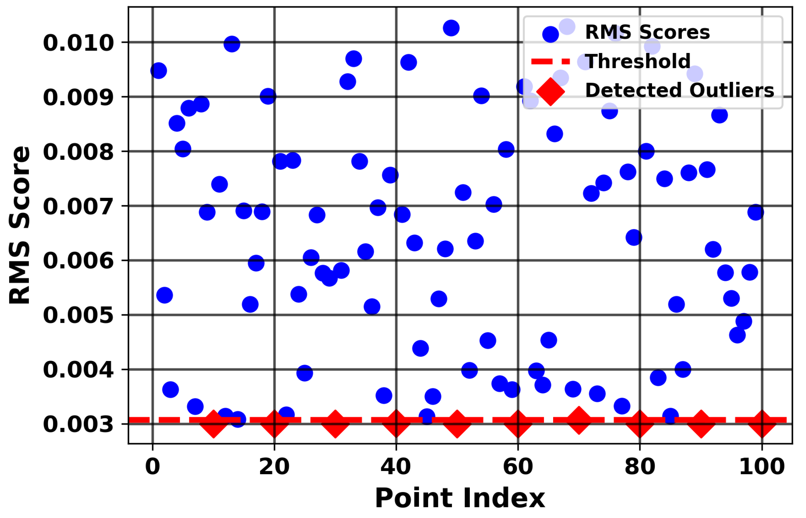
The intuition is that inliers, being embedded within the main data cluster, maintain non-negligible interactions with multiple neighbors, resulting in relatively high RMS scores. In contrast, outliers, separated from the bulk of the data, yield predominantly near-zero bias interactions, producing markedly lower RMS scores.

Threshold Criterion for Outlier Assignment

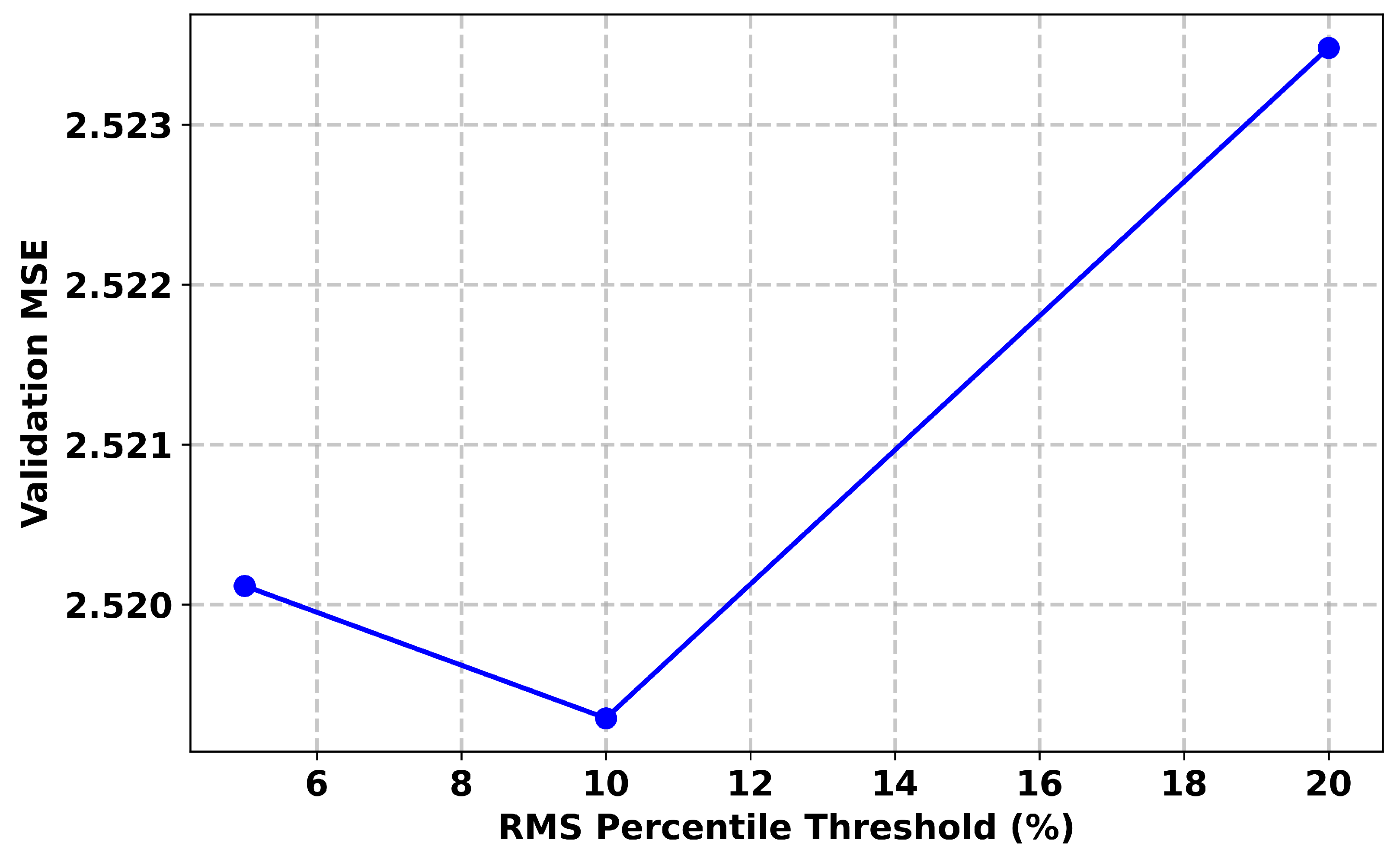
To translate the RMS scores into a detection decision, we adopt a percentile-based thresholding strategy. Specifically, a point is classified as an outlier if its RMS score falls below the 10th percentile of the RMS score distribution. We tested multiple RMS percentile thresholds (5%, 10%, 20%) for outlier identification and found that the 10% cutoff consistently yielded the lowest validation Mean Square Error (MSE). The blue circles in Figure 4 represent the Mean Square Error (MSE) values obtained at different RMS percentile thresholds during validation. Specifically, the 5%, 10%, and 20% thresholds yielded MSEs of approximately 2.520, 2.519, and 2.523, respectively, supporting the selection of 10% for our analysis. This RMS-based approach provides a practical method for bias thresholding, rather than relying on arbitrary cutoff values.

In the synthetic dataset, the 10th percentile corresponded to an RMS score of approximately 0.02. Thus, points with

$$\mathrm{RMS}\left(i\right)<0.02$$

(17)

Were flagged as outliers.

Figure 5 illustrates the distribution of RMS scores for all 100 data points. A clear separation can be observed between inliers and outliers, with outliers concentrated in the lower tail of the distribution. Using the 10th percentile threshold ≈ (0.02), the method successfully flagged the originally injected outliers at indices 10, 20, 40, 50, 60, 70, 80, 90, and 100. Interestingly, an additional point at index 83 was also detected as an outlier, highlighting the sensitivity of the proposed RMS-based approach in capturing unexpected deviations beyond the predefined anomalies.

3.3. Downweighting Outliers Using a Weight Vector in SVR

Following the identification of outliers using the bias-values-based RMS scoring method, we incorporated a weighting scheme [20] to mitigate their impact during model training. Rather than removing the outliers from the dataset, which could discard potentially useful information, we employed a sample-specific weight vector [21,22] to control the contribution of each point to the SVR optimization.

Let

$$\mathbf{w}=\left[\begin{array}{c}{w}_1\\ w_2\\ ⋮\\ w_N\end{array}\right]$$

denote the weight vector, where N is the total number of samples. Each element $w_i$ corresponds to the i-th sample in the training dataset and is assigned as follows:

$$w_i=\left\{\begin{array}{cc}ϵ,\hfill & \mathrm{if} x_i \mathrm{is} \mathrm{detected} \mathrm{as} \mathrm{an} \mathrm{outlier}\hfill \\ 1,\hfill & \mathrm{otherwise} (\mathrm{normal} \mathrm{sample})\hfill \end{array}\right.$$

Here, $ϵ$ is a small positive value (0.001) obtained by Bayesian optimization Section 3.4, the weight vector determines how much the outliers are downweighted, effectively reducing their influence in SVR optimization while retaining their presence in the dataset. Normal samples retain full weight, ensuring that the model prioritizes the bulk of the data during regression.

In MATLAB version R2025a, this weight vector is supplied to the fitrsvm function through the ‘Weights’ parameter, allowing the SVR solver to scale the $ϵ$-insensitive loss for each sample proportionally.

By adopting this approach, the regression model becomes robust to extreme deviations, as the optimization process essentially “ignores” the outliers while still leveraging all available data. This method preserves the structural information of the dataset, aligns with the kernel-based outlier-detection framework, and complements the bias-matrix methodology by ensuring that identified outliers exert minimal influence on the learned SVR function. The SVR loss function is given by

$$\begin{array}{cc}& \underset{w,b,\xi ,{\xi }^{*}}{min}{\displaystyle \frac{1}{2}}{\parallel w\parallel }^2+C\sum _{i=1}^n({\xi }_i+{\xi }_i^{*})\hfill \\ & \mathrm{subject} \mathrm{to}:\hfill \\ & y_i-\left(w^{\top }\varphi \left(x_i\right)+b\right)\le ϵ+{\xi }_i,i=1,\dots ,n,\hfill \\ & \left(w^{\top }\varphi \left(x_i\right)+b\right)-y_i\le ϵ+{\xi }_i^{*},i=1,\dots ,n,\hfill \\ & {\xi }_i\ge 0,{\xi }_i^{*}\ge 0,i=1,\dots ,n.\hfill \end{array}$$

In subsequent sections of this work, we will utilize this SVR formulation as the baseline method for our simulations and comparisons with the proposed method. This will allow us to evaluate the effectiveness of our approach, in particular the outlier-detection technique presented in Section 3, and its impact on the SVR framework.

3.4. Bayesian Optimization Hyperparameter Selection

Bayesian optimization is an algorithm that efficiently explores the hyperparameter space to find optimal values for the model. To ensure the optimal performance of the BT-SVR, we applied Bayesian optimization to systematically tuning key hyperparameters for the kernels (RBF and Polynomial) used in our simulations.

In our setup, the kernel bandwidth ($\sigma$) for the RBF kernel, the degree (d) for the polynomial kernel, the regularization term (C) and epsilon ($ϵ$) for the model were selected through Bayesian optimization. The optimization process was conducted over 30 iterations, evaluating different configurations to identify the most effective set of parameters.

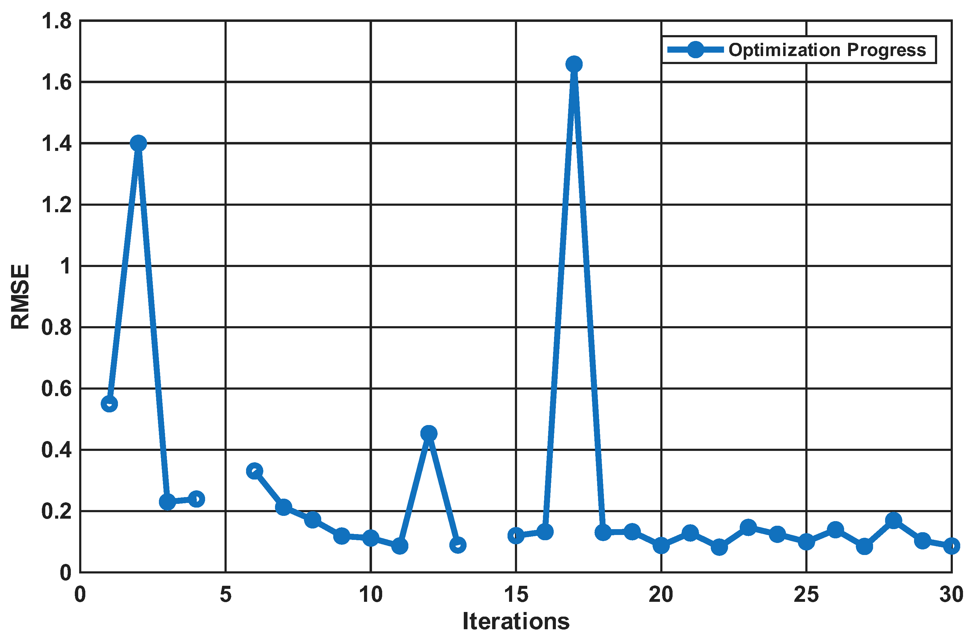
To visualize the optimization process for the hyperparameter search, we plotted the number of iterations against the RMSE. Figure 6 illustrates the RMSE values over 30 iterations of the Bayesian optimization process. The plot shows how the algorithm explores a wide range of parameter combinations within the specified bounds, with fluctuations in the curve reflecting its evaluation of diverse configurations.

3.5. Software and Computational Setup

All simulations and numerical experiments were performed using MATLAB R2025a (MathWorks, Natick, MA, USA) and Python 3.13.0 (tags/v3.13.0:60403a5, 7 October 2024, 09:38:07) [MSC v.1941 64 bit (AMD64)] on a Windows 10 (64-bit) operating system. The implementation of the proposed BT-SVR model, including the bias term for outlier detection and robust regression, was carried out in MATLAB using the Optimization Toolbox, while visualization was conducted in Python.

All computations were executed on a DESKTOP-OG3L04L system equipped with an Intel^® Core™2 Duo CPU P7550 @ 2.26 GHz, 4.00 GB of RAM (3.75 GB usable), and a 238 GB Apacer A S350 SSD. The system does not support pen or touch input.

4. Simulation Results

The dataset used for experimentation and performance evaluation of the BT-SVR method, consists of historical stock data for the S&P 500 index, covering the period from 29 January 1993–24 December 2020 see

Table 1. S&P 500 Stock Data.

Date	Open	High	Low	Close	Volume
29 January 1993	43.96875	43.96875	43.75	43.9375	1,003,200
1 February 1993	43.96875	44.25	43.96875	44.25	480,500
2 February 1993	44.21875	44.375	44.125	44.34375	201,300
⋮	⋮	⋮	⋮	⋮	⋮
29 December 2006	141.88	142.47	141.0	141.62	151,605,600
⋮	⋮	⋮	⋮	⋮	⋮
21 December 2020	364.97	378.46	362.03	367.86	96,386,700
22 December 2020	368.21	368.33	366.03	367.24	47,949,000
23 December 2020	368.28	369.62	367.22	367.57	46,201,400
24 December 2020	368.08	369.03	367.45	369.0	26,457,900

.

This dataset, obtained from Kaggle (S&P 500 Dataset https://www.kaggle.com/datasets/camnugent/sandp500) (accessed on 8 October 2025), provides a rich and detailed time series of financial data, making it highly suitable for predictive modeling tasks in Support Vector Regression (SVR). Importantly, stock market data frequently contains abrupt fluctuations and irregular patterns, which often manifest as outliers. This characteristic makes the dataset particularly appropriate for assessing the effectiveness of the proposed method, especially in handling noisy or anomalous observations.

The dataset includes six features, as outlined in Table 1:

• Date: The trading date of the record.
• Open: The opening price of the S&P 500 index on the given date.
• High: The highest price reached during the trading day.
• Low: The lowest price reached during the trading day.
• Close: The closing price of the index on the given date.
• Volume: The trading volume, representing the number of shares traded on that day.

The “close” (closing price) column 5 in Table 1 serves as the target variable for prediction.

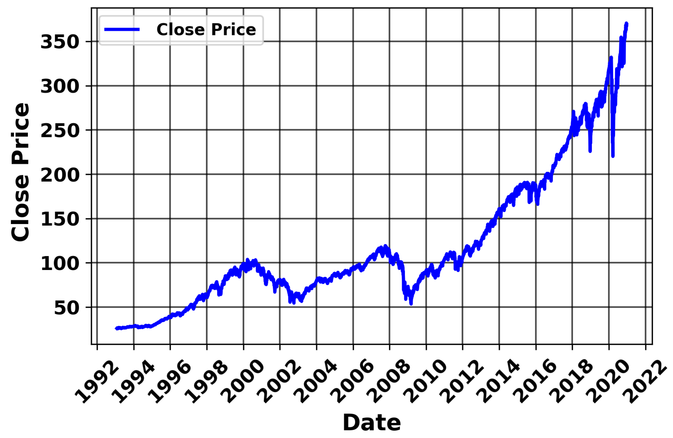
The S&P 500 Close Price plot Figure 7 highlights the non-linear nature of financial data, characterized by significant fluctuations and irregular trends. It also reveals the presence of outliers caused by major economic events. These complexities make this dataset ideal for testing the robustness of our proposed and outlier detection technique. For the simulation, we utilized a dataset of 7029 samples from the S&P 500, with five features, excluding the date column from Table 1. The data was split into 80% (5623) for training and 20% for testing (1405). The model was evaluated using the Root Mean Square Error (RMSE) metric, and we employed a Radial Basis Function (RBF) kernel for the simulation. For the bias matrix computation, we used the following parameters:

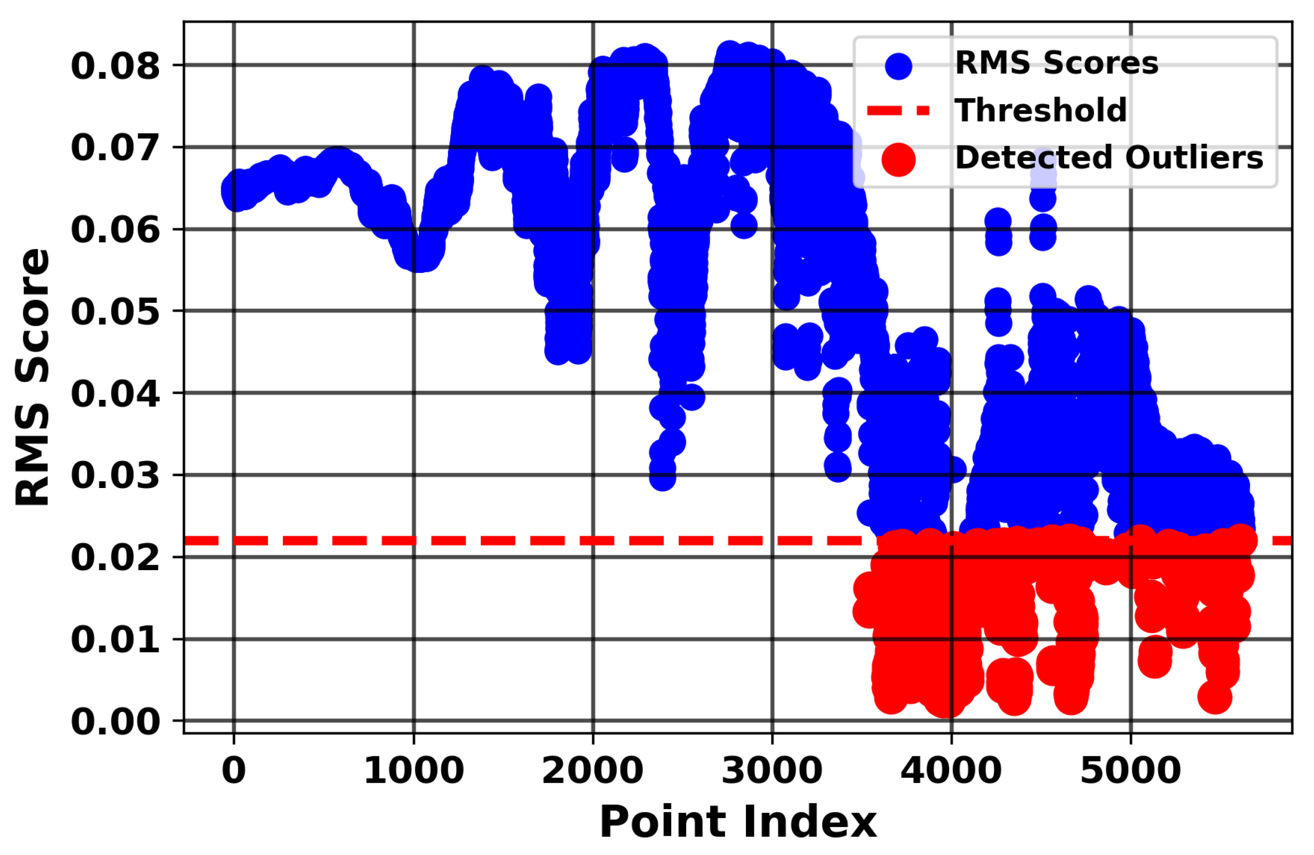
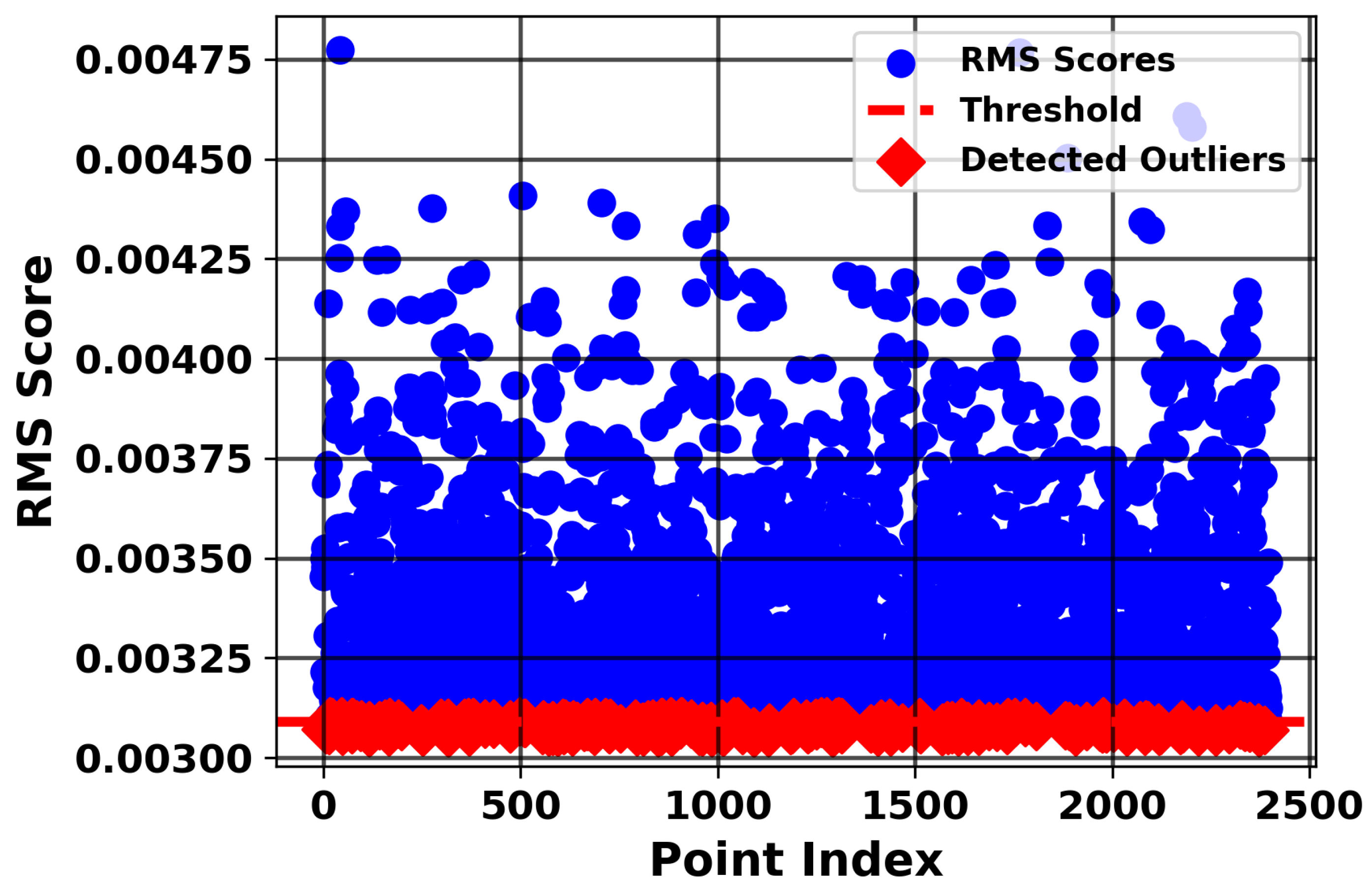
Sigma ($\sigma =1$), (noise term ${\sigma }_{\eta }=0.4330$, representing the mean variance of all features), and $d=5$ (the number of feature dimensions). For training, the model was configured with $C=84.031$ and $ϵ=0.002$. In Figure 8, we identified outliers from the bias values using an RMS threshold established at the 10th percentile, precisely calculated as 0.021989 based on the distribution of RMS scores across the dataset. This threshold was determined by analyzing the RMS scores derived from the bias values, which quantifies the deviation of each data point from the expected behavior under a kernel-based similarity model. Samples exhibiting RMS scores below this dashed threshold line, as visually depicted in Figure 8, were flagged as outliers, indicating potential anomalies or noise in the S&P 500 data. This process resulted in a total of 562 detected outliers, representing approximately 8% of the training samples, which aligns with the expectation of capturing a small but significant portion of anomalous data points given the large dataset of 7029 samples. After identifying these outliers, we utilized their indices to systematically track and manage their impact on the subsequent modeling process. To achieve this, we constructed a weight vector w, a 1 × N array where N corresponds to the number of rows in the training samples, ensuring a one-to-one mapping with each data point. This weighting approach was designed to mitigate the influence of outliers while enhancing the model’s focus on inliers.

Specifically, we assigned $w=0.001$ to the indices corresponding to the outliers, effectively downweighting their contribution to the training process to reduce their disproportionate effect on the model’s fit. Conversely, we set $w=1$ for inliers, maximizing their impact and signaling the model to prioritize these representative data points during training.

This strategic weighting scheme was implemented to guide the Support Vector Regression (SVR) model with RBF kernel toward learning from the more reliable inlier patterns, thereby improving the robustness and predictive accuracy of the model.

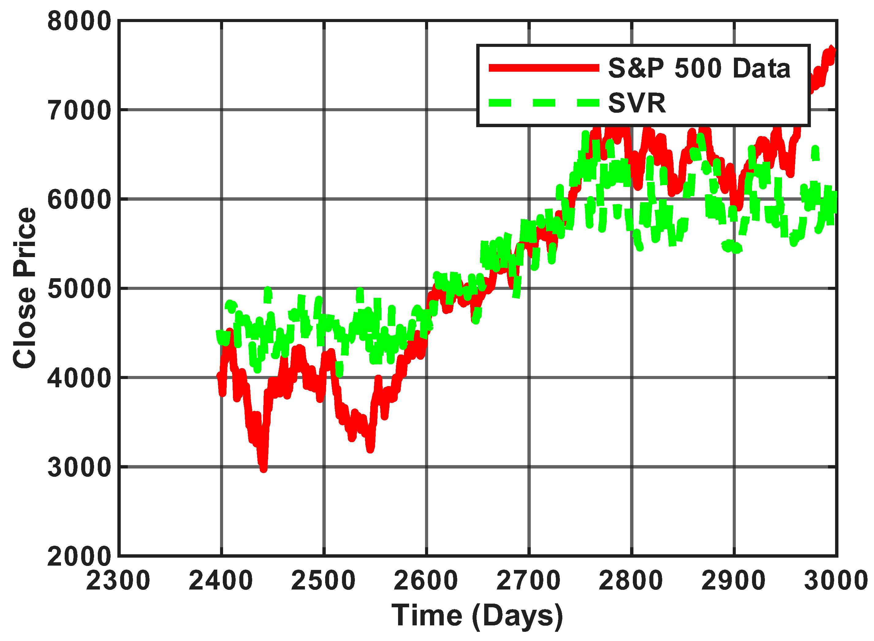
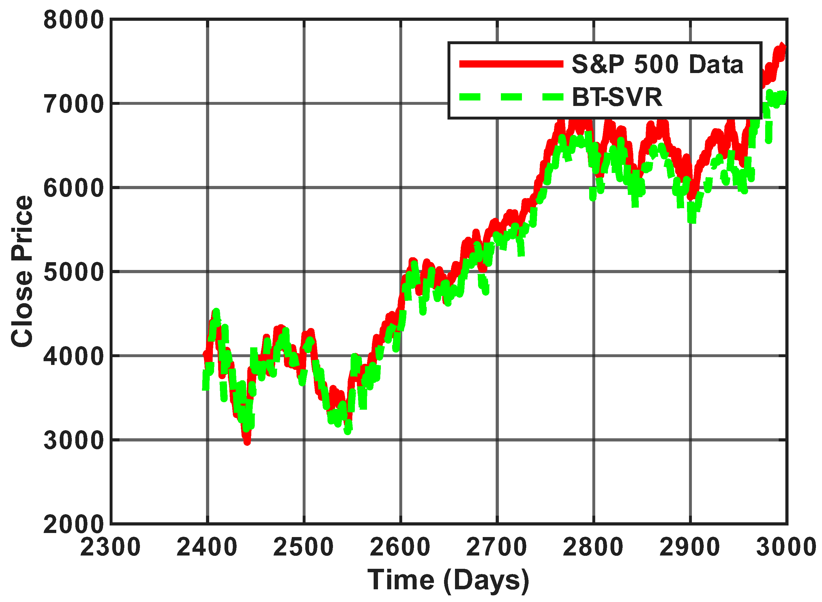
The simulation results reveal that the proposed bias-based outlier detection method substantially improves predictive accuracy compared to the baseline SVR model. Specifically, the SVR without outlier handling achieved an RMSE of 0.3441, while the proposed method reduced the error to 0.0641. The results represent an approximate 81% reduction in prediction error, highlighting the effectiveness of the BT-SVR strategy in mitigating the influence of anomalous samples.

The marked improvement can be attributed to the ability of the proposed method to detect and downweight outliers before model training. By assigning lower weights to noisy or anomalous data points, the regression model was guided to prioritize the structural patterns in the majority of the data, thereby enhancing robustness. In contrast, the standard SVR treated all samples equally, making it more sensitive to irregular fluctuations and extreme deviations in the dataset.

Overall, these results summarized in Figure 9 and Figure 10 demonstrate that the integration of the bias term into the learning process leads to a more reliable regression model, capable of achieving higher predictive accuracy in the presence of noisy or irregular financial time series data.

Experiment II

To evaluate the robustness and adaptability of BT-SVR further, we conducted an additional experiment using another real-world dataset, the Combined Cycle Power Plant (CCPP) dataset, and used a polynomial kernel for training the model, in contrast to the RBF kernel used in the first experiment. In this case, the Mean Squared Error (MSE) metric was used for performance evaluation, and the results were compared against those of Huber regression, a well-established robust outlier technique. The dataset (CCPP) from the UCI Machine Learning Repository [23] contains 9568 samples collected from a power plant operating at full load for six years (2006–2011).

It includes four features and one target variable.

• Ambient Temperature (AT);
• Exhaust Vacuum (V);
• Ambient Pressure (AP);
• Relative Humidity (RH);

One target variable: Net Hourly Electrical Energy Output (PE), measured in megawatts (MW).

For our experiments, the dataset is split into 80% training (7654 samples) and 20% testing (1914 samples). The simulation aims to predict the energy output of the machine using the BT-SVR method and Huber regression. Following the methodology established in Section 3, the bias term was applied to detecting outliers in the CCPP dataset. Figure 11 illustrates the RMS scores of the bias values from the CCPP dataset. The red diamonds indicate training points identified as outliers based on their RMS scoring weights, which are approximately around 0.003, while the blue circles represent inlier samples with weights above the defined threshold. Bayesian optimization, as described in Section 3.4, was used to select the hyperparameters. The parameters of the bias term are sigma ($\sigma =2.236$) (noise term ${\sigma }_{\eta }=1$, representing the mean variance in all features) and $d=5$ (the number of feature dimensions). For training, the model was configured with $C=10$ $ϵ=0.1$ and degree (d = 2) for the polynomial kernel. This process identified 240 outliers—see Figure 11—corresponding to approximately 3.1% of the training set, which were subsequently downweighted by $w=0.001$ to enhance the model’s robustness. Huber regression was implemented using the “robustfit” function in MATLABR2025a.

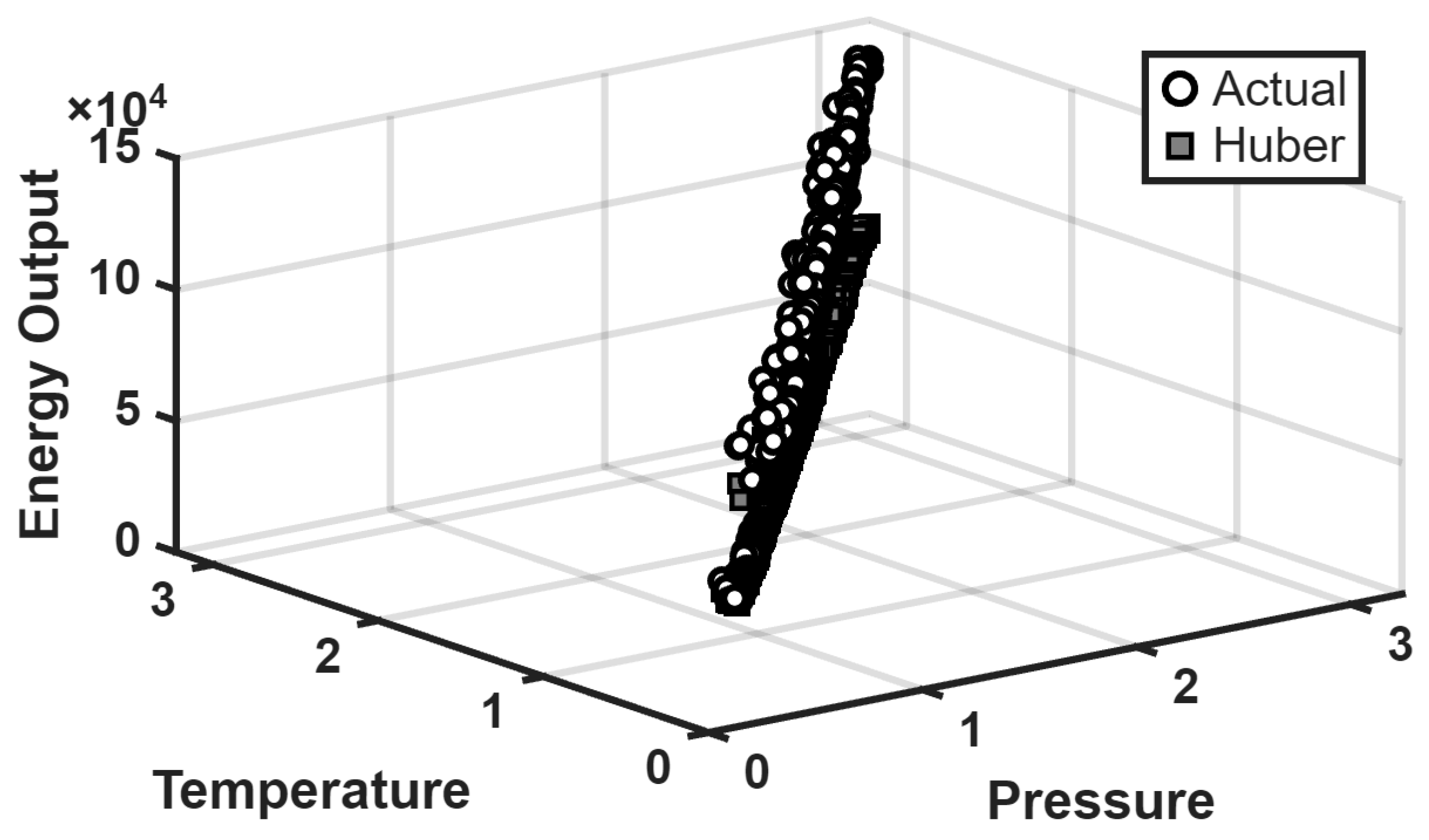
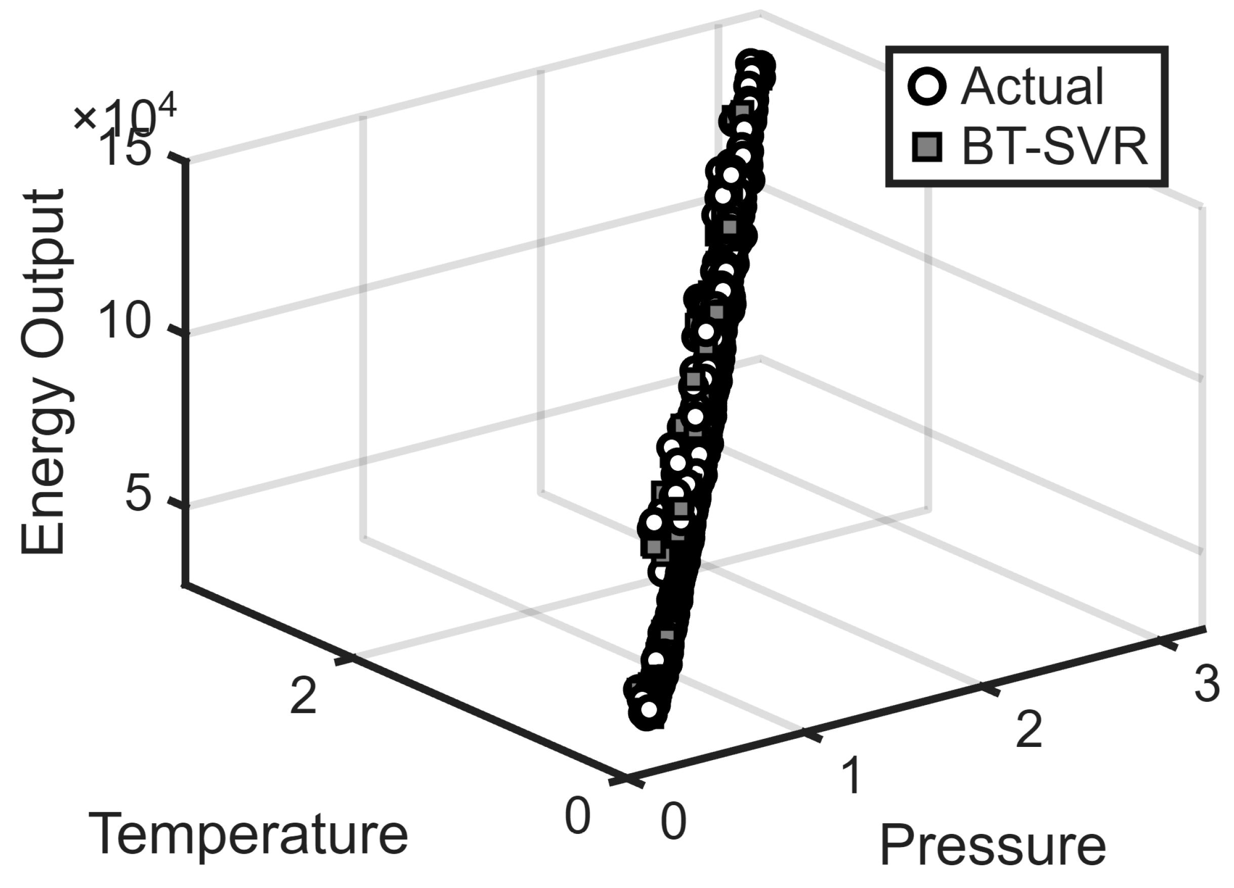
Figure 12 displays the predictive performance of Huber regression on the testing set. The results indicate noticeable deviations between the predicted and actual energy outputs, leading to a Mean Squared Error (MSE) of 0.9752. In contrast, Figure 13 presents the outcome of BT-SVR, where the predictions align more closely with the observed values. The BT-SVR achieved a substantially lower MSE of 0.2220, reflecting an improvement compared to Huber regression. These findings demonstrate that BT-SVR provides more accurate and robust predictions in the presence of outliers. The incorporation of the bias term for outlier suppression, combined with the SVR framework, contributes to enhanced generalization and stability relative to conventional robust regression.

5. Parameter Impact on Model Performance

In this section, we examine the impact of key hyperparameters on the performance of the BT-SVR method, evaluated using the CCPP dataset from Experiment II. Specifically, we vary the hyperparameters ($\sigma$) (where ($\gamma ={\displaystyle \frac{1}{2{\sigma }^2}}$)), (C), and ($ϵ$) to assess their influence on the BT-SVR model’s performance, measured via the Mean Squared Error (MSE). Additionally, we incorporate the polynomial kernel, as utilized in Experiment II, to train the model and evaluate the sensitivity of the BT-SVR method to these variations.

5.1. Gamma $\left(\gamma \right)$ Parameter

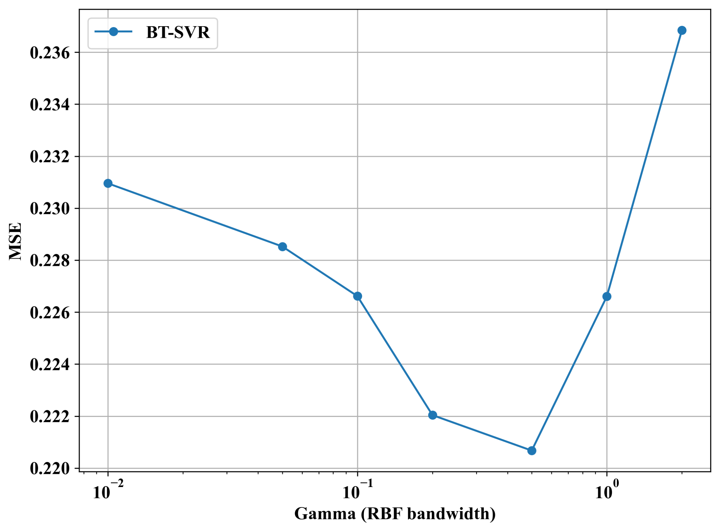
The sensitivity of the BT-SVR method to the gamma parameter ($\gamma =1/\left(2{\sigma }^2\right)$, where $\sigma$ is the kernel bandwidth) is a critical factor in optimizing model performance, particularly in outlier detection and robust regression. Figure 14 illustrates the Mean Squared Error (MSE) as a function of $\gamma$, varied logarithmically from ${10}^{-2}$ to ${10}^0$. This analysis evaluates how $\gamma$ influences the bias term’s effectiveness and the overall robustness of the model against noisy data and outliers.

The MSE exhibits a U-shaped trend, with an optimal range around $\gamma \approx {10}^{-1}$ (0.1), where the error reaches a minimum of approximately 0.222. This suggests that a moderate $\gamma$ value effectively balances the Gaussian RBF kernel’s sensitivity to pairwise Euclidean distances and the bias term’s ability to capture structural information for outlier detection. As $\gamma$ increases from ${10}^{-2}$ to ${10}^{-1}$, the MSE decreases, indicating improved generalization as the kernel captures more relevant data relationships, aligning with the exponential decay property discussed in Section 3.

At low $\gamma$ values (e.g., ${10}^{-2}$), the MSE rises to around 0.23, suggesting underfitting. A small $\gamma$ corresponds to a narrow kernel, making it excessively sensitive to noise and reducing the bias term’s discriminative power. This is consistent with the kernel’s asymptotic behavior, where $K(\tilde{u},\tilde{v})\to 0$ exponentially for a large value of ${\parallel \delta \parallel }^2$, overwhelming the bias contribution and limiting the outlier detection efficacy. Conversely, at high $\gamma$ values (e.g., ${10}^0$ and beyond), the MSE increases sharply to 0.236 and higher, indicating overfitting. A large $\gamma$ value widens the kernel, assigning significant weight to distant pairs, which dilutes the bias term’s ability to isolate outliers and reduces the model’s robustness, as the RMS scores become less discriminative.

The transition point around $\gamma \approx {10}^0$ highlights the model’s high sensitivity to $\gamma$ beyond this threshold. The sharp MSE increase suggests that careful tuning of $\gamma$ is essential to maintain the balance between the kernel width and the bias term.

For practical implementation, $\gamma$ should be tuned around ${10}^{-1}$, using hyperparameter selection algorithms, to leverage the bias term’s discriminative power while ensuring SVR stability and achieving a low prediction error. Future experiments could explore $\gamma$’s interaction with the noise variance ${\sigma }_{\eta }^2$ and weight parameter $ϵ$ to optimize the performance further across diverse datasets.

5.2. C Parameter

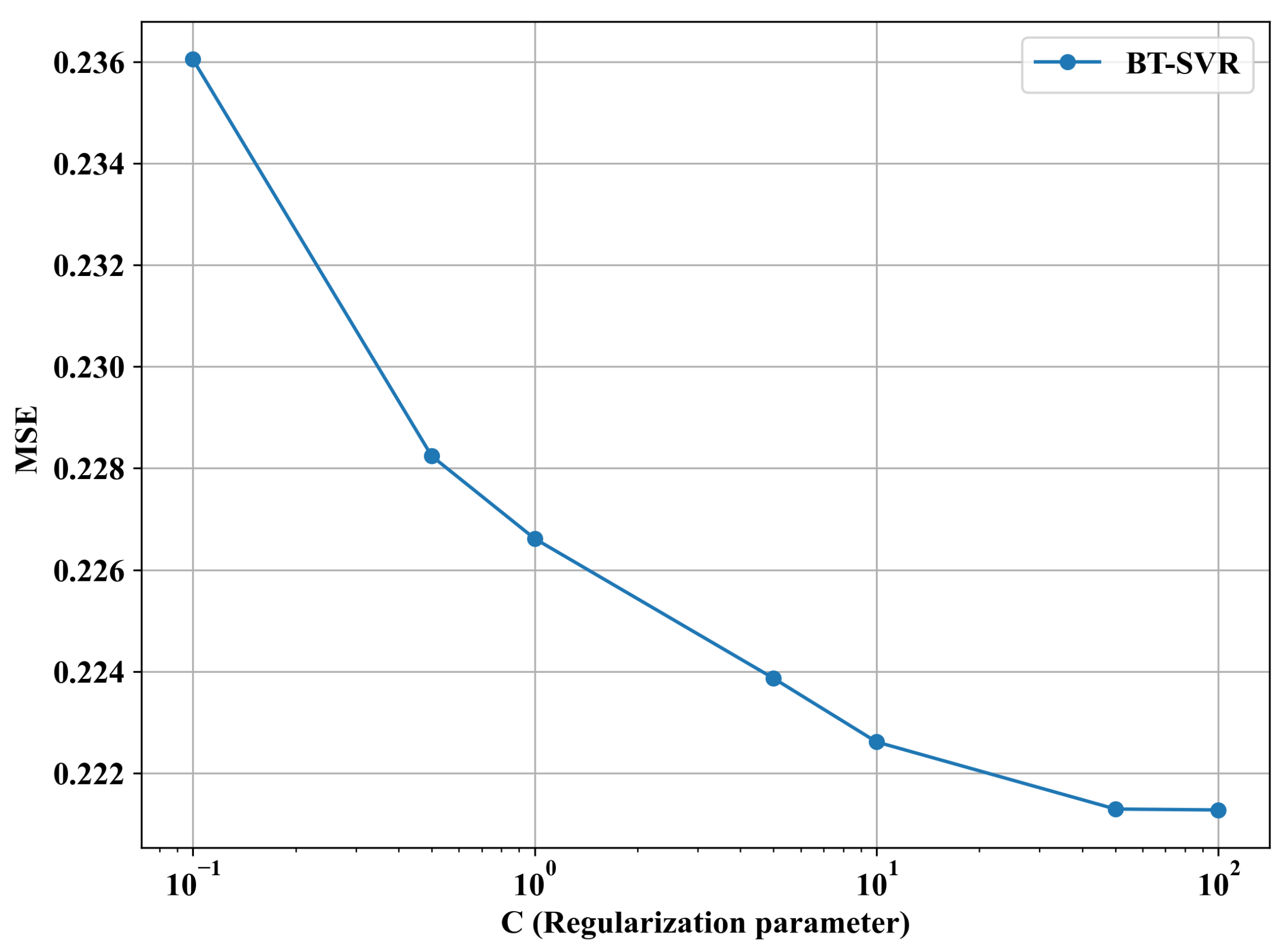
The regularization parameter C in the BT-SVR method plays a pivotal role in controlling the trade-off between model complexity and the penalty for errors, directly influencing the robustness of SVR against noisy data and outliers. Figure 15 presents the Mean Squared Error (MSE) as a function of C, varied logarithmically from ${10}^{-1}$ to ${10}^2$. This analysis assesses how C affects the bias term’s outlier detection capability and the overall model performance.

The MSE exhibits a decreasing trend as C increases from ${10}^{-1}$ to approximately ${10}^1$ (10), where it stabilizes around a minimum of approximately 0.222. At $C={10}^{-1}$, the MSE is highest at 0.236, indicating underfitting, as a small C imposes a strong regularization penalty, limiting the model’s ability to fit the training data, including the downweighted outliers identified by the RMS scoring mechanism in Section 3. As C increases to ${10}^0$ (1) and ${10}^1$ (10), the MSE decreases steadily, suggesting that a moderate to higher value for C allows the model to capture the underlying data relationships better.

Beyond $C\approx {10}^1$, the MSE remains relatively stable around 0.222, indicating that further increases in C (e.g., to ${10}^2$) have diminishing returns. This plateau suggests that the model has reached an optimal balance where the penalty for outliers is sufficiently mitigated and additional regularization relaxation does not significantly improve the fit. However, excessively large C values could risk overfitting by over-emphasizing training data points, including noisy ones, although this is not evident within the plotted range.

The sensitivity of the MSE to C is most pronounced between ${10}^{-1}$ and ${10}^1$, where a ten-fold increase in C reduces the error by approximately 0.014. This highlights the importance of tuning C within this interval using hyperparameter selection algorithms to achieve a robust performance. Future studies could investigate the interaction between C and heteroscedastic noise to enhance the model’s robustness further across diverse datasets.

5.3. Epsilon ($ϵ$) Parameter

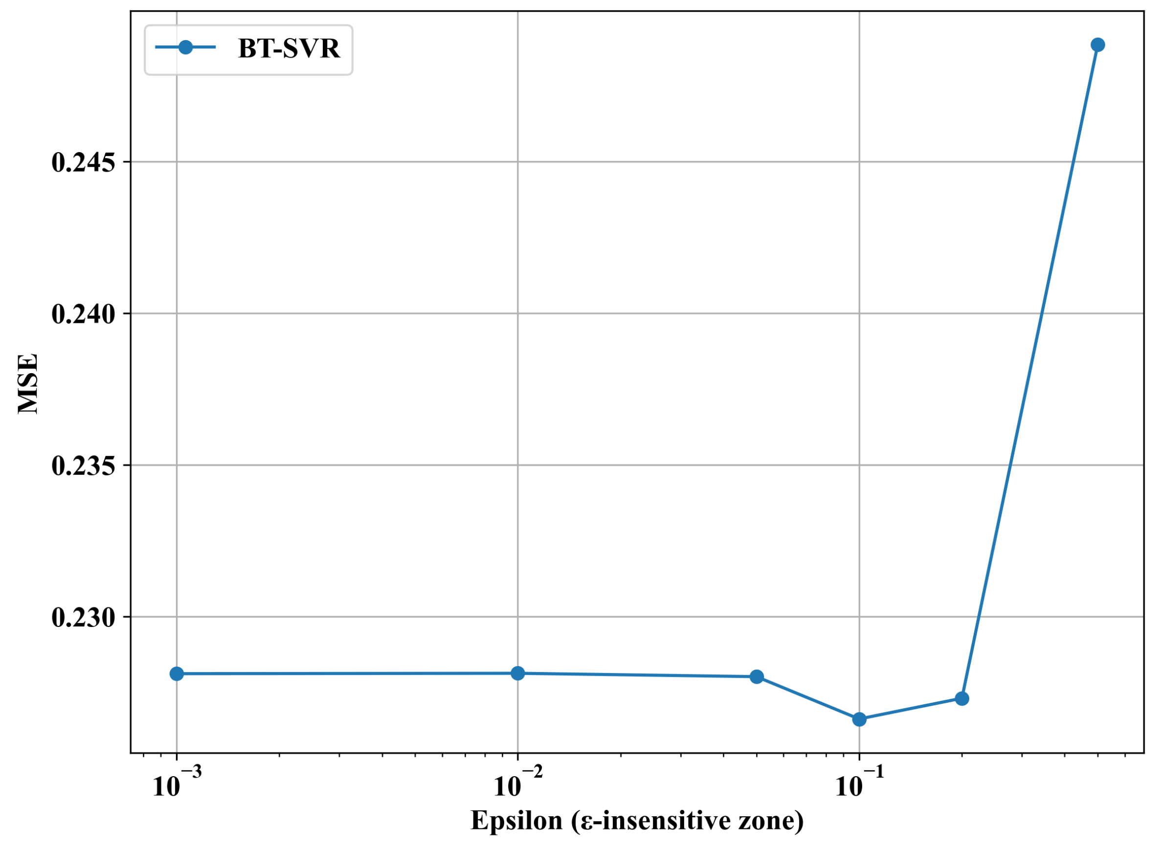
The epsilon ($ϵ$) parameter in the BT-SVR method defines the $ϵ$-insensitive zone, a key component of Support Vector Regression (SVR) that determines the margin within which errors are not penalized. This parameter significantly influences the model’s robustness to noisy data and outliers by interacting with the bias term’s outlier detection mechanism. Figure 16 presents the Mean Squared Error (MSE) as a function of $ϵ$, varied logarithmically from ${10}^{-3}$ to ${10}^1$. This analysis examines how $ϵ$ affects the balance between model fit and tolerance for deviations, particularly in the context of the RMS-based outlier downweighting strategy.

The MSE remains relatively stable and low, around 0.230, for $ϵ$ values ranging from ${10}^{-3}$ to ${10}^{-1}$, indicating that small $ϵ$ values effectively minimize errors within the $ϵ$-insensitive zone. The optimal performance is observed around $ϵ\approx {10}^{-1}$ (0.1), where the MSE dips slightly to approximately 0.228. This suggests that a moderate $ϵ$ allows the model to tolerate small residuals while leveraging the bias term’s structural information to downweight outliers identified via RMS scoring.

As $ϵ$ increases beyond ${10}^{-1}$, the MSE begins to rise, reaching approximately 0.245 at $ϵ={10}^0$ (1) and climbing sharply to over 0.245 at $ϵ={10}^1$ (10). This upward trend indicates overfitting, as a larger $ϵ$ widens the insensitive zone, reducing the model’s sensitivity to errors and allowing more outliers to fall within the margin without penalty. This diminishes the effectiveness of the bias term and downweighting, leading to poorer generalization.

For practical implementation, $ϵ$ should be tuned in the range of ${10}^{-3}$ to ${10}^{-1}$, with a hyperparameter selection technique recommended to identify the optimal value. This range ensures the BT-SVR maintains a tight $ϵ$-insensitive zone, enhancing robustness against noisy data.

6. Limitations of the Proposed Method

Despite its strong empirical performance, the proposed method has several limitations:

• Noise assumptions: The derivation assumes isotropic, Gaussian, and independent noise, whereas real-world data may exhibit heteroscedasticity, heavy tails, or dependence.
• Independence assumption: The current framework treats data points as i.i.d., which overlooks temporal dependencies common in sequential datasets such as financial returns.
• Computational complexity: The bias matrix requires $O\left(N^2\right)$ operations, which is not scalable to very large datasets. For instance, when $N=7029$, the bias matrix involves nearly 49 million entries, making computation expensive. Approximate kernel methods such as Nyström approximation or sampling-based strategies could be explored to address this limitation.
• Generalizability: While experiments on stock data and the CCPP dataset demonstrate robustness, the method has not yet been formally extended to explicitly incorporate volatility clustering or non-Gaussian effects.

7. Conclusions

This work introduces a novel bias-based approach for robust regression and outlier detection in Support Vector Regression (SVR). By deriving a bias term from the second-order Taylor expansion of the Gaussian RBF kernel and utilizing its relationship with pairwise input distances, the proposed method identifies and downweights anomalous samples. This was demonstrated in financial time series data the “S&P 500” and the “CCPP” dataset. Unlike traditional pre-processing or filtering techniques, the BT-SVR framework retains all data points while adaptively reducing the influence of outliers, thus preserving the structural information of the data set. The proposed method offers advantages over the SVR and Huber regression model, showcasing its robustness against irregular fluctuations and noisy samples.. By minimizing the disproportionate impact of anomalies, it guides the regression model to prioritize reliable patterns, enhancing predictive accuracy and generalization. These attributes position it as a promising tool for financial forecasting and other domains, such as healthcare, engineering, and autonomous systems, where noisy and anomalous data often impair regression performance. In summary, incorporating the bias term into the regression process provides a principled and effective solution for mitigating outlier effects. The improvements achieved affirm the method’s potential as a general framework for strengthening robustness in kernel-based learning.

8. Future Work

Future work will explore extending this approach to other kernel functions, applying it to high-dimensional datasets, and integrating it with deep kernel learning frameworks for broader applicability. A promising direction for future research is to extend the BT-SVR framework beyond the i.i.d. assumption to better handle sequential and dependent data. In particular, temporal dependencies could be incorporated through lagged features or embedding techniques that explicitly capture time series dynamics prior to applying the bias-based weighting scheme. Additionally, adapting the framework to volatility-aware models, such as GARCH-inspired formulations or time-varying kernels, would improve its robustness in domains like financial forecasting, where heteroscedasticity and clustering effects are common.

References

- Mohammed, S.; Budach, L.; Feuerpfeil, M.; Ihde, N.; Nathansen, A.; Noack, N.; Patzlaff, H.; Harmouch, H.; Naumman, F. The Effects of Data Quality on Machine Learning Performance. arXiv 2022, arXiv:2207.14529. [Google Scholar] [CrossRef]
- Zhang, X.; Wei, P.; Wang, Q. A hybrid anomaly detection method for high dimensional data. PeerJ Comput. Sci. 2023, 9, e1199. [Google Scholar] [CrossRef] [PubMed]
- Rajkomar, A.; Dean, J.; Kohane, I. Machine Learning in Medicine. N. Engl. J. Med. 2019, 380, 1347–1358. [Google Scholar] [CrossRef] [PubMed]
- Patel, J.; Shah, S.; Thakkar, P.; Kotecha, K. Predicting Stock Market Index Using Fusion of Machine Learning Techniques. Expert Syst. Appl. 2015, 42, 2162–2172. [Google Scholar] [CrossRef]
- Bojarski, M.; Testa, D.D.; Dworakowski, D.; Firner, B.; Flepp, B.; Goyal, P.; Jackel, L.D.; Monfort, M.; Muller, U.; Zhang, J.; et al. End to End Learning for Self-Driving Cars. arXiv 2016, arXiv:1604.07316. [Google Scholar] [CrossRef]
- Bablu, T.A.; Mirzaei, H. Machine Learning for Anomaly Detection: A Review of Techniques and Applications in Various Domains. J. Comput. Soc. Dyn. 2025, 7, 1–25. Available online: https://www.researchgate.net/publication/389038707_Machine_Learning_for_Anomaly_Detection_A_Review_of_Techniques_and_Applications_in_Various_Domains (accessed on 8 October 2025).
- Sabzekar, M.; Hasheminejad, S.M.H. Robust Regression Using Support Vector Regressions. Chaos Solitons Fractals 2021, 144, 110738. [Google Scholar] [CrossRef]
- Adelusi, J.B.; Thomas, A. Data Cleaning and Preprocessing for Noisy Datasets: Techniques, Challenges, and Solutions. Technical Report, 2025. Available online: https://www.researchgate.net/publication/387905797_Data_Cleaning_and_Preprocessing_for_Noisy_Datasets_Techniques_Challenges_and_Solutions (accessed on 8 October 2025).
- Teng, C.M. Evaluating Noise Correction. In Proceedings of the PRICAI 2000: Pacific Rim International Conference on Artificial Intelligence, Melbourne, Australia, 28 August–1 September 2000; Springer: Berlin/Heidelberg, Germany, 2000; pp. 188–198. [Google Scholar] [CrossRef]
- Cui, W.; Yan, X. Adaptive weighted least square support vector machine regression integrated with outlier detection and its application in QSAR. Chemom. Intell. Lab. Syst. 2009, 98, 130–135. [Google Scholar] [CrossRef]
- Chen, X.; Yang, J.; Liang, J.; Ye, Q. Recursive robust least squares support vector regression based on maximum correntropy criterion. Neurocomputing 2012, 97, 63–73. [Google Scholar] [CrossRef]
- Chen, C.; Li, Y.; Yan, C.; Guo, J.; Liu, G. Least absolute deviation-based robust support vector regression. Knowl. Based Syst. 2017, 131, 183–194. [Google Scholar] [CrossRef]
- Hu, J.; Zheng, K. A novel support vector regression for data set with outliers. Appl. Soft Comput. 2015, 31, 405–411. [Google Scholar] [CrossRef]
- Liu, J.; Wang, Y.; Fu, C.; Guo, J.; Yu, Q. A robust regression based on weighted LSSVM and penalized trimmed squares. Chaos Solitons Fractals 2016, 89, 328–334. [Google Scholar] [CrossRef]
- Chen, C.; Yan, C.; Zhao, N.; Guo, B.; Liu, G. A robust algorithm of support vector regression with a trimmed Huber loss function in the primal. Soft Comput. 2017, 21, 5235–5243. [Google Scholar] [CrossRef]
- García, S.; Luengo, J.; Herrera, F. Data Preprocessing in Data Mining; Intelligent Systems Reference Library; Springer: Cham, Switzerland, 2015; Volume 72, pp. 107–133. [Google Scholar] [CrossRef]
- Smola, A.J.; Schölkopf, B. A tutorial on support vector regression. Stat. Comput. 2004, 14, 199–222. [Google Scholar] [CrossRef]
- Stewart, J. Calculus: Early Transcendentals, 9th ed.; Cengage Learning: Boston, MA, USA, 2016. [Google Scholar]
- Magnus, J.R.; Neudecker, H. Matrix Differential Calculus with Applications in Statistics and Econometrics, 3rd ed.; Wiley: Chichester, UK, 1999. [Google Scholar]
- Xie, M.; Wang, D.; Xie, L. A Feature-Weighted SVR Method Based on Kernel Space Feature. Algorithms 2018, 11, 62. [Google Scholar] [CrossRef]
- Shantal, M.; Othman, Z.; Abu Bakar, A. A Novel Approach for Data Feature Weighting Using Correlation Coefficients and Min–Max Normalization. Symmetry 2023, 15, 2185. [Google Scholar] [CrossRef]
- Muthukrishnan, R.; Kalaivani, S. Robust Weighted Support Vector Regression Approach for Predictive Modeling. Indian J. Sci. Technol. 2023, 16, 2287–2296. [Google Scholar] [CrossRef]
- Dua, D.; Graff, C.; Tüfekci, P.; Kaya, H. Combined Cycle Power Plant Data Set. UCI Machine Learning Repository. Available online: https://archive.ics.uci.edu/dataset/294/combined+cycle+power+plant (accessed on 8 October 2025).