Article

Bearing Fault Diagnosis Using PSO-VMD and a Hybrid Transformer-CNN-BiGRU Model

1
School of Computer and Information Engineering, Tianjin Chengjian University, Tianjin 300383, China
2
Hangzhou Zhijiang Switchgear Stock Co., Ltd., Hangzhou 311203, China
*
Author to whom correspondence should be addressed.
Symmetry 2025, 17(11), 1780; https://doi.org/10.3390/sym17111780
Submission received: 24 September 2025 / Revised: 15 October 2025 / Accepted: 16 October 2025 / Published: 22 October 2025
(This article belongs to the Section Engineering and Materials)

Abstract

Reliable bearing fault diagnosis is essential for the steady running of mechanical systems. However, existing diagnostic models still face significant limitations in feature extraction, primarily due to the non-stationary and nonlinear characteristics of vibration signals, which lead to a decline in diagnostic performance. To address this issue, this paper proposes a novel diagnostic framework that combines Particle Swarm Optimization-based Variational Mode Decomposition (PSO-VMD) for feature extraction with a deeply integrated Transformer-Convolutional Neural Network-Bidirectional Gated Recurrent Unit (TCB) model for fault classification. Bearing fault diagnosis is crucial for the stable operation of mechanical equipment, yet existing models often suffer from limited feature extraction and low detection accuracy. To address this, PSO-VMD is employed to extract informative, band-limited features from vibration signals, yielding a highly correlated feature set; a composite model TCB, combining a Transformer, a CNN, and a bidirectional GRU (BiGRU), is then used for fault classification. To prevent window-level leakage, the dataset is split before windowing and normalization, and all baselines are aligned under identical preprocessing and training settings. On the CWRU benchmark, the model attains 98.9% accuracy, 98.8% precision, 99.4% recall, 99.1% F1, and macro-F1 = 0.9766 over five runs. The approach offers a favorable accuracy –latency trade-off and yields interpretable, band-limited modes, supporting reproducible deployment in practice.

1. Introduction

With the continuous advancement of industrialization, ensuring the reliability of bearings has become an increasingly severe challenge. The increase in bearing failure rates poses a major threat to equipment operation and overall production efficiency. Bearing failures can lead to severe consequences, including equipment damage [1], production downtime, economic losses, and even personal injuries [2]. Therefore, bearing fault diagnosis has become a crucial approach to ensuring the reliable operation of equipment and maintaining production safety [3].
Research on bearing fault diagnosis primarily focuses on extracting features from vibration signals and developing fault diagnosis models [4]. With the increasing diversity of fault types and modes, bearing vibration signals have become increasingly complex, often accompanied by noise interference and redundant information. To address this challenge, researchers have extensively studied feature extraction methods for bearing vibration signals. Early approaches relied on manual extraction, which resulted in low recognition accuracy [5]. Dong HB et al. [6] proposed a motor-bearing fault diagnosis approach that employs information –entropy features derived from Empirical Mode Decomposition (EMD), which improved recognition accuracy. However, when modal aliasing occurs in vibration signal processing, it can result in insufficient feature extraction and error accumulation, ultimately affecting the accuracy of the diagnosis results. Zou P et al. [7] employed ensemble empirical mode decomposition (EEMD) to derive features from the raw signal by injecting white noise, effectively reducing the occurrence of modal aliasing. Although EEMD performs better than EMD, it requires adding noise and reconstructing the signal multiple times, which increases the computational complexity. Ding et al. [8] proposed a Variational Mode Decomposition (VMD) algorithm to separate the signal’s distinct frequency components without adding noise or performing repeated reconstructions. However, the performance of VMD depends on the penalty factor α and the number of decomposition modes K, making parameter selection challenging when relying solely on manual experience. This study applies Particle Swarm Optimization to tune the parameters of Variational Mode Decomposition. The optimized VMD is then utilized to extract features from the bearing dataset, enhancing the model’s classification accuracy.
Song et al. [9] employed a Support Vector Machine (SVM) to enhance prediction accuracy by identifying the optimal decision boundary. Zhou J B et al. [10] optimized the hyperparameters of SVM, enhancing its global search capability in complex feature spaces. H. Wang B et al. [11] employed multi-scale symbolic entropy combined with the whale optimization algorithm to obtain a low-dimensional embedding of the original high-dimensional data, thereby enhancing the bearing fault classification model. However, when handling nonlinear data, the inappropriate selection of the SVM kernel function can result in suboptimal classification accuracy. Additionally, the model struggles to capture the spatial and temporal dependencies inherent in time series data, leading to potential performance limitations. Deep learning models have proven effective in capturing intricate features and signal patterns, offering a robust solution to the limitations of SVM when processing nonlinear and time series data. Shao et al. [12] introduced a 1D convolutional neural network (1D-CNN) and assessed it on the Case Western Reserve University (CWRU) bearing dataset. The results demonstrated that the 1D-CNN model outperformed traditional machine learning methods in terms of classification accuracy and overall performance. Chen et al. [13] employed a real-world bearing vibration dataset to conduct a comparative analysis between traditional machine learning techniques and deep learning models. The results revealed that the deep learning model achieved superior classification accuracy and overall performance compared to traditional machine learning models. Notably, it demonstrated significant advantages in handling complex nonlinear fault signals, highlighting its effectiveness in fault diagnosis tasks. However, simple CNN models are prone to overfitting when processing time series data [14]. These models are limited in their ability to capture only short-term local features and fail to effectively model long-term dependencies. As a result, they tend to overfit to the local features present in the training data, leading to reduced generalization performance on unseen data. To address these challenges, Yan et al. [15] proposed an optimization based on the CNN-GRU model. By integrating CNN for feature extraction and GRU for processing temporal information, the model’s performance was enhanced. However, the GRU component processes information unidirectionally, neglecting future context. This limitation can lead to overfitting, as the model may fail to fully capture the temporal dependencies in both directions. Xu et al. [16] put forward a bearing fault diagnosis technique that leverages a CNN-BiGRU model, where the BiGRU module enhances the model’s ability to capture both forward and backward temporal information, thus reducing the risk of overfitting. However, when processing long sequences, the model struggles to capture subtle changes in fault characteristics. It tends to focus on local information, which may lead to inaccurate detection of the fault occurrence time, thereby impacting the overall accuracy of fault diagnosis. An et al. [17] proposed a bearing fault diagnosis approach built on a periodic sparse attention mechanism, which enhanced diagnostic accuracy by concentrating on the key areas of periodic changes in long sequences. However, this approach exhibited limited adaptability to non-periodic faults, making it less effective in handling faults that do not exhibit regular patterns. Yang et al. [18] introduced a bearing fault diagnosis approach using a signal transformation neural network (SiT) combined with pure AM. This approach improved diagnostic performance by enhancing the model’s adaptability to non-periodic faults. However, it still faces the challenge of overemphasizing local information, which may hinder its ability to capture global contextual features crucial for accurate fault diagnosis. Zhou et al. [19] introduced the Transformer model, which effectively captures long-distance dependencies in data and identifies non-adjacent complex faults. This approach addresses the issue of local information bias, significantly improving fault diagnosis accuracy. While Transformer excels in capturing long-range dependencies and mitigating local bias, it has not yet been combined with the CNN-BiGRU model, leaving an opportunity for further enhancement in fault diagnosis performance.
Building upon the research findings and analyses presented above, this paper introduces and integrates an improved PSO algorithm, VMD, CNN module, BiGRU, and Transformer module to propose an efficient bearing fault diagnosis model. This model addresses the challenges of feature extraction and model construction in bearing fault diagnosis, ultimately enabling more accurate and efficient fault detection. By leveraging the strengths of each component, the proposed model enhances the overall diagnostic performance, particularly in handling complex fault patterns and long-range dependencies in the data.
The main research gaps of this study are as follows:
Most existing methods treat signal decomposition and fault classification as separate processes, lacking a unified optimization mechanism, which affects the effectiveness of feature extraction and classification performance.
Many models struggle to handle both non-periodic fault signals and long-term temporal dependencies simultaneously, often leading to overfitting and insufficient fault localization accuracy.
The main contributions of this paper are as follows:
A PSO optimized VMD method was proposed to adaptively obtain optimal decomposition parameters, thereby enhancing the effectiveness of feature decomposition and ensuring a symmetric separation of modal components.
A hybrid deep learning model integrating Transformer, CNN, and BiGRU architectures was constructed to strengthen the joint modeling capability of spatial and temporal features of vibration signals. This design maintains a structural symmetry by balancing global–local and forward–backward temporal representations.
The proposed model supports end-to-end optimization and demonstrates higher diagnostic accuracy and generalization capability across various fault scenarios, while achieving a symmetric trade-off among accuracy, convergence speed, and computational efficiency.

2. Experiment

2.1. Dataset Introduction

This research makes use of the bearing dataset provided by Case Western Reserve University (CWRU), which includes signals corresponding to a healthy bearing condition and three distinct fault types: inner race fault, outer race fault, and rolling element fault. Degradation mechanisms such as wear, corrosion, and fracture can lead to different bearing fault states. The experimental setup used for acquiring vibration signals under operational conditions is depicted in Figure 1. The public download link (https://engineering.case.edu/bearingdatacenter) (accessed on 23 September 2025). is now included to facilitate reproducibility for other researchers.

2.2. Data Selection

In this analysis, acceleration data from the drive end (DE) of an SKF bearing was employed. The rotational speed is maintained at 1797 revolutions per minute (rpm), with a sampling rate of 12 kHz. The bearings used in the experiment contain single-point defects with three different sizes: 0.007, 0.014, and 0.021 inches in diameter, as detailed in Table 1.
Note: All samples were collected under a constant speed of 1797 r/min and no load (0 N), resulting in identical values in the corresponding columns.
To enhance the diagnostic performance of the proposed model, a systematic and targeted data preprocessing strategy was applied to the input signals prior to training. The specific steps are as follows:
Data slicing and label generation:
The entire dataset was first loaded, and a sliding window technique was used to segment the original time-series signal into fixed-length subsequences. Each subsequence was then assigned its corresponding fault label, which was subsequently converted into a one-hot encoded format to support multi-class classification tasks.
Data normalization:
All signal values within the subsequences were normalized to mitigate the impact of inconsistent dimensionality, thereby improving the uniformity of feature distributions and facilitating model convergence.
Dataset partitioning:
Post preprocessing, the data were distributed across training, validation, and test sets in a 6:2:2 proportion. This ensured scientific rigor and reproducibility throughout model training and evaluation. We use a split-before-windowing protocol. The train/validation/test split is performed at the raw-record (condition) level (defined by load, speed, fault location, and fault size). After the split, sliding-window segmentation and normalization are applied within each subset only. All windows from the same raw record are assigned to a single subset to prevent window-level leakage.
This preprocessing strategy not only improved the consistency of model inputs and classification performance, but also established a stable foundation for subsequent feature extraction and learning.
We use a unified preprocessing pipeline for all methods. The train/validation/test split is performed before windowing at the raw-record (condition) level. Z-score normalization parameters are fitted on the training split only and reused for validation and test. PSO–VMD is applied with the same configuration (number of modes K, penalty α, PSO settings),where hyper-parameters are tuned solely on the training/validation data to prevent leakage. From the IMFs we extract an identical feature vector (time–and frequency-domain statistics, envelope-spectrum peaks, spectral entropy, kurtosis, RMS, energy, etc.), and this feature vector is used for all comparator models and for our method.

2.3. Feature Extraction

The Variational Mode Decomposition (VMD) algorithm involves two critical parameters [20], K and α Here, K denotes the number of intrinsic mode functions (IMFs) into which the signal is decomposed, representing the number of modal components. The α serves as a constraint factor that controls the smoothness of each mode after decomposition. Selecting appropriate values for K and α is essential to ensure the effectiveness and accuracy of the VMD process. To address this, an improved Particle Swarm Optimization (PSO) algorithm is employed in this study to optimize these parameters. The two core equations of the PSO algorithm are as follows:
v i j ( t + 1 ) = w v i j ( t ) + c 1 r 1 ( x i j p ( t ) x i j ( t ) ) + c 2 r 2 ( x i j G ( t ) x i j ( t ) )
x i j ( t + 1 ) = x i j ( t ) + v i j ( t + 1 )
Here v i j ( t ) is the velocity of particle i on dimension j   x i j ( t ) is the personal best of particle i and x i j G ( t ) is the global best. w is the inertia factor; c 1 and c 2 are acceleration factors.; r 1 and r 2 are random numbers in the interval [0, 1]. t represents the number of iterations. Each particle in the swarm is represented as follows: x i j = { x i 1 , x i 2 , , x i n } , i = 1 , 2 , , m . The velocity of each particle is updated by the following formula: v i j = { v i 1 , v i 2 , , v i n } , i = 1 , 2 , , m .
The value of the inertia weight w significantly influences the motion behavior of the particle. The acceleration coefficients c 1 and c 2 play a critical role in determining the exploration and exploitation capabilities of the particle swarm. Therefore, in this study, all three parameters w , c 1 , and c 2 are improved to enhance the overall performance of the algorithm. The improvement strategy is described as follows:
w ( k ) = w max ( w max w min ) ( k / g e n s ) 2
c 1 = c 1 s + ( c 1 e c 1 s ) ( k / g e n s )
c 2 = c 2 s + ( c 2 e c 2 s ) ( k / g e n s )
where k denotes the current iteration number, c 1 is the cognitive learning factor scheduled by linear interpolation from c 1 s (start) to c 1 e (end). c 2 is the social learning factor scheduled by linear interpolation from c 2 s to c 2 e . w max denotes the maximum inertia weight, and w min denotes the minimum, and is the maximum number of iterations.
During the iterative process, When c 1 s > c 1 e and c 2 s < c 2 e , a larger self-learning factor combined with a smaller social-learning factor enhances the particles’ self-exploration capability while reducing their reliance on group experience. This configuration promotes more effective global search during the optimization process.
To balance global exploration and local exploitation during the iterative process, the inertia weight ω is linearly decreased from 0.9 to 0.4. In addition, the cognitive acceleration factor c1 and the social acceleration factor c2 are dynamically adjusted according to the number of iterations, enabling a gradual transition from individual exploration to global convergence. This strategy helps mitigate the premature convergence problem of the particle swarm and enhances the robustness of the PSO optimization process.
Variational Mode Decomposition (VMD) is a novel signal processing technique proposed by Konstantin Dragomiretskiy in 2014 [20]. This method adaptively determines the number of modes based on the characteristics of the input signal and assigns each mode a corresponding center frequency and finite bandwidth. As a result, the original signal can be efficiently broken down into a series of intrinsic mode functions (IMFs). The specific steps of the VMD algorithm are as follows:
(1)
Solve the constrained variational model to perform signal decomposition. The constrained variational model is formulated as follows:
min { u k , w k } k t δ ( t ) + j π t u k ( t ) e j w k t 2 2 s . t . k u k = f ( t )
In the equation, f t represents the original signal, and δ t + j π t u k t denotes u k t ‘s Hilbert transform. u k , w k are the optimization variables, u k ( t ) is the k-th intrinsic mode function (IMF).
(2)
Introduce the quadratic penalty factor α and the Lagrange multiplier λ t to convert the constrained variational model into an unconstrained one:
L ( { u k } , { ω k } , λ ) = α k t ( δ ( t ) + j π t ) u k ( t ) e j w k t 2 2 + f ( t ) k u k ( t ) 2 2 + λ ( t ) , f ( t ) k u k ( t )
(3)
Apply the Alternating Direction Method of Multipliers (ADMM) to iteratively update u k n + 1 , ω k n + 1 , λ k n + 1 in order to obtain the saddle point of the Lagrangian expression. The expression is given as follows:
u k n + 1 ( ω ) = f ( ω ) i k u i ( ω ) + λ ( ω ) 2 1 + 2 α ( ω ω k ) 2
ω k n + 1 = 0 ω u k ( ω ) 2 d ω 0 u k ( ω ) 2 d ω
λ n + 1 ( ω ) = λ n ( ω ) + τ f ( ω ) k u k n + 1 ( ω )
(4)
The VMD iteration terminates when the decomposed modes satisfy the convergence condition defined in Equation (8).
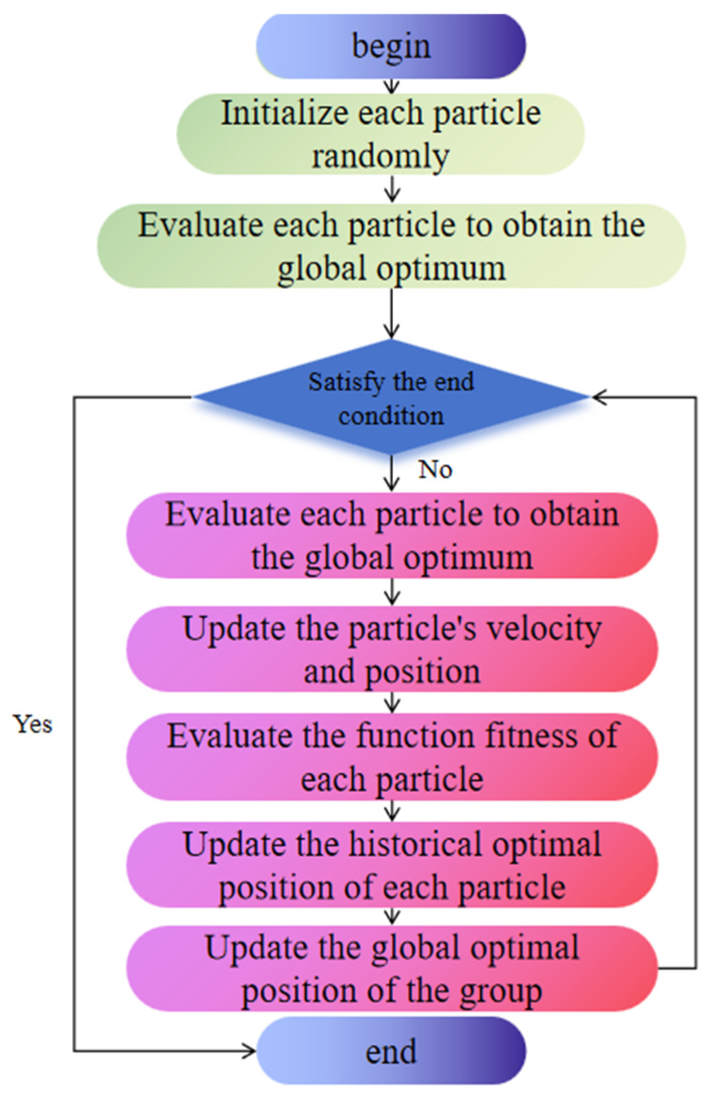
Particle Swarm Optimization (PSO) is a heuristic optimization algorithm inspired by the collaborative and information-sharing behavior of birds when searching for food. It finds the optimal solution by continuously updating and optimizing the positions of particles through iterative processes. PSO has been widely applied in areas such as signal processing and vibration analysis. By employing the PSO algorithm to adaptively optimize the VMD parameters [K,α], the influence of human intervention can be minimized. The basic process of PSO is illustrated in Figure 2.
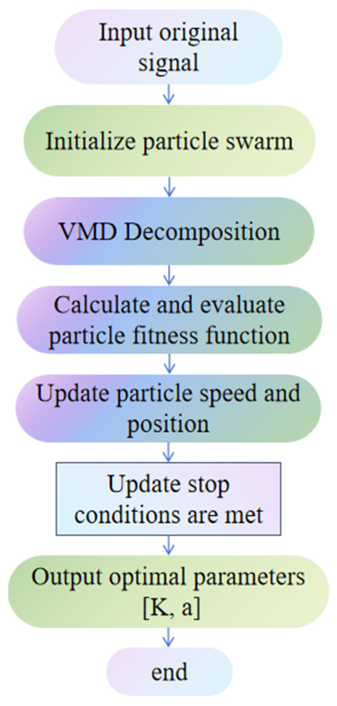
The PSO-VMD parameter optimization process (Figure 3) is as follows:
(1)
Set the initial parameters of the PSO algorithm, including the cognitive coefficient c 1 (local search ability), the social coefficien c 2 (global search ability), the maximum number of iterations Tmax, and the velocity-position relationship coefficient K, among others.
(2)
Use the local minimum entropy value under random conditions as the fitness value of the particle swarm optimization algorithm. Perform Variational Mode Decomposition (VMD) on the original signal, and compute and record the Ecmfe value of each Intrinsic Mode Function (IMF) along with the corresponding particle position.
(3)
Compare the local minimum entropy values at each particle position, select the smallest one, and update both the individual particle’s best-known (local) minimum entropy value and the global minimum entropy value of the entire population accordingly.
(4)
Update each particle’s velocity and position based on the individual best and global best solutions.
(5)
Return to Step 3 and repeat the process until the maximum number of iterations is reached. Then, output the optimal fitness value along with the corresponding parameters α and K.
(6)
Output: The optimal parameter combination corresponding to the global best position is determined.
In the PSO-VMD optimization process, the initial parameters of the PSO algorithm are set as follows: number of particles: 20. maximum number of iterations: 50. inertia weight (ω): linearly decreasing from 0.9 to 0.4. The cognitive factor (c1) and the social factor (c2) are both initialized at 1.5 but are dynamically adjusted throughout the iterations. These parameter settings are based on commonly used empirical values in signal decomposition and optimization tasks, offering a good balance between convergence speed and global search capability.

2.4. Fault Diagnosis Model

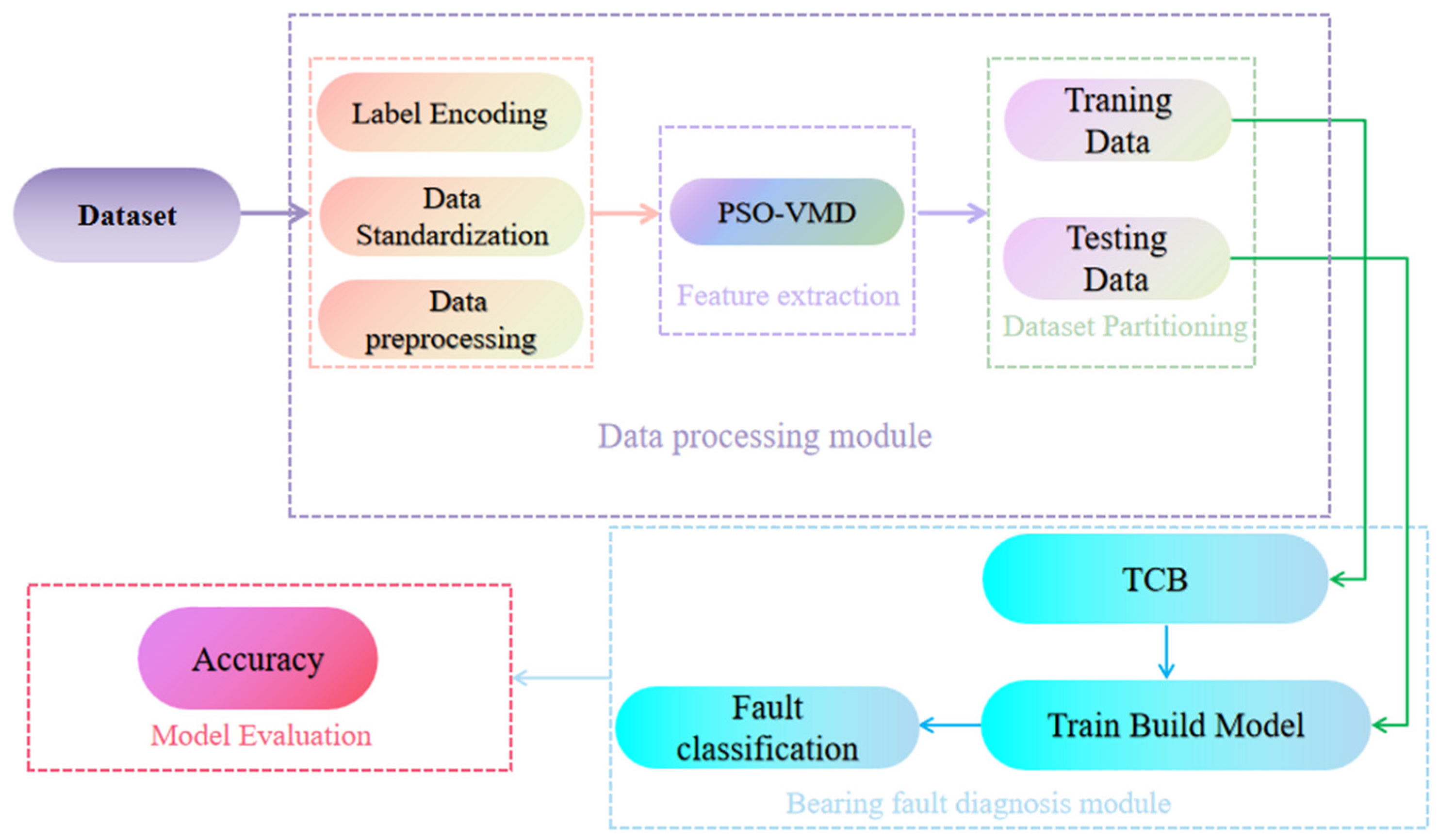
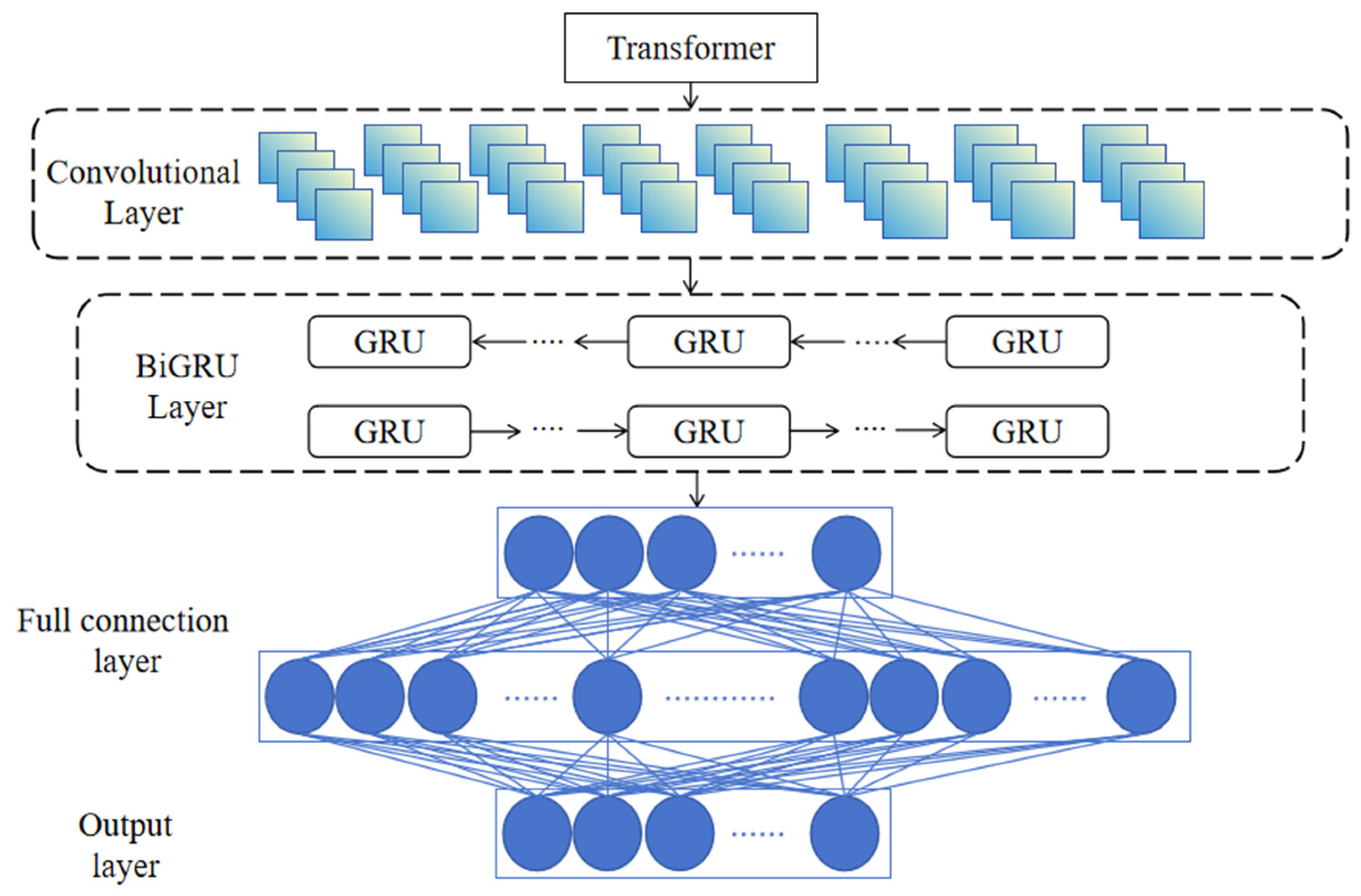
The bearing fault diagnosis model proposed in this paper consists of two main modules: a data processing module and a fault diagnosis module. The data processing module includes three components: data preprocessing, feature extraction, and dataset partitioning. The core of the fault diagnosis module is the Transformer-CNN-BiGRU model, which integrates the Transformer, Convolutional Neural Network (CNN), and Bidirectional Gated Recurrent Unit (BiGRU) architectures for effective classification of bearing faults. The overall workflow of the model is illustrated in Figure 4.

2.4.1. Transformer

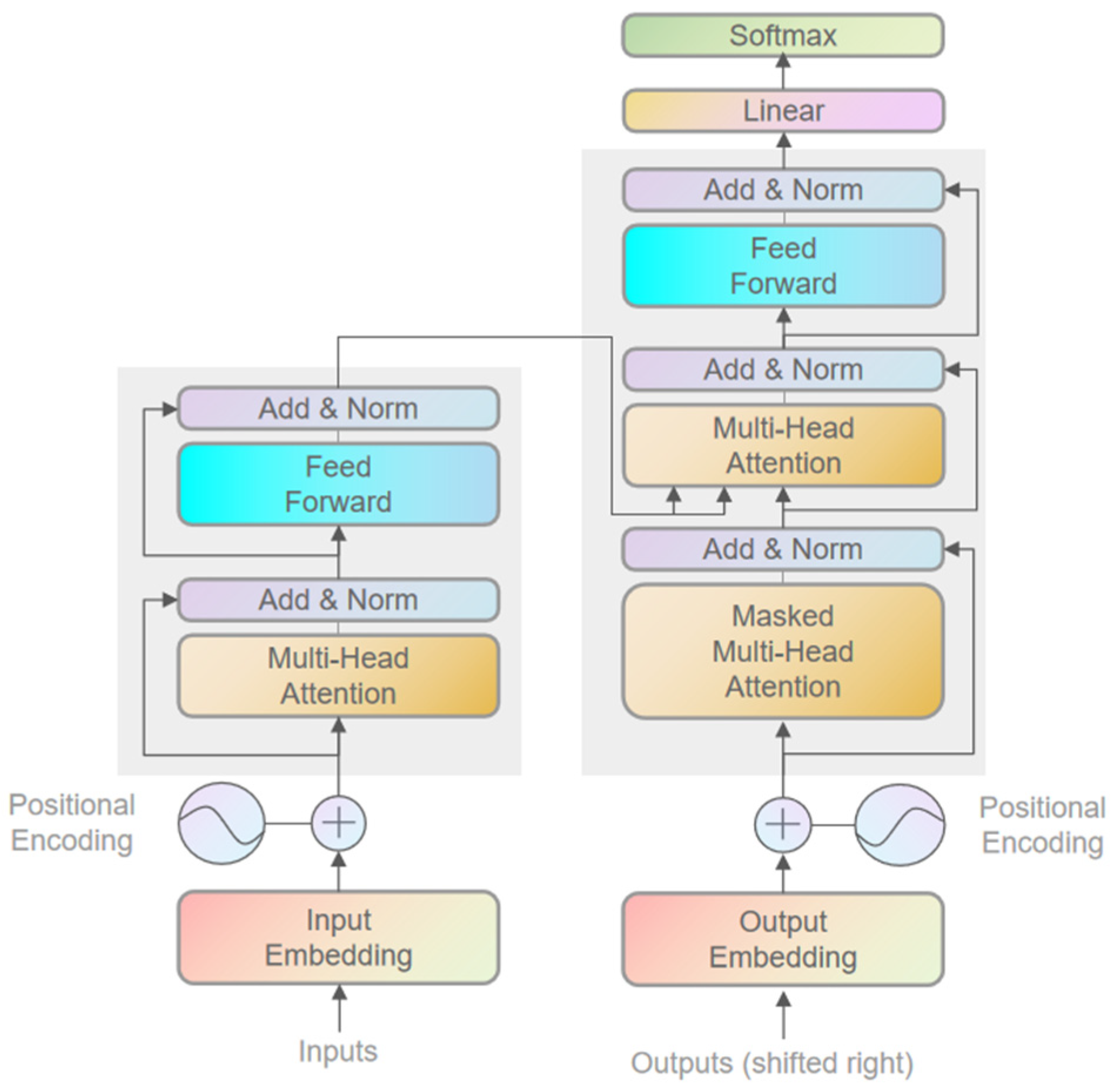
The Transformer module adopts an encoder-decoder architecture (Figure 5). The encoder transforms the input sequence into a contextual representation, while the decoder generates the output sequence based on the context provided by the encoder. By introducing a multi-head self-attention mechanism, the Transformer replaces the traditional recurrent neural network (RNN) structure, enabling efficient parallel computation.
The multi-head self-attention mechanism identifies key regions within the input sequence and reinforces the information in these regions by computing the correlations between each element and all other elements in the sequence. Specifically, the self-attention mechanism generates attention weights by calculating the similarity between the query, key, and value vectors, and then performs a weighted summation of the input sequence to produce the output representation. The multi-head structure enhances the model’s representation capability by computing multiple attention heads in parallel, allowing the model to capture different types of contextual information from various subspaces.

2.4.2. CNN

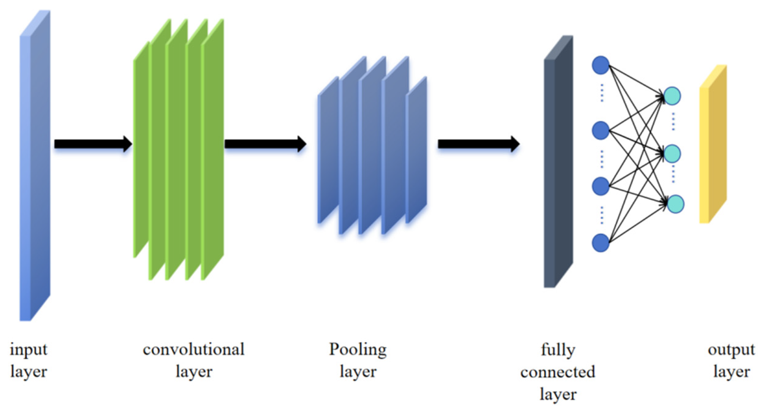
Convolutional Neural Networks (CNN) were originally developed for image processing tasks [21]. With the advancement of research, CNN have been widely applied to time series analysis. In regression tasks, CNN primarily serve to extract local fluctuations and short-term features from time series data through convolution operations. These features are then progressively integrated to support the prediction of continuous values. The structural diagram of the CNN is shown in Figure 6. Suppose the time series dataset is D, which contains the sample set X = { x 1 , x 2 , x 3 , , x m } and the corresponding labels Y = { y 1 , y 2 , y 3 , , y m } . Each sample x 1 is represented as a time series of length l, that is, X i = { x i 1 , x i 2 , x i 3 , , x i n } . In the convolution layer, the convolution kernel slides along the input sequence to extract local features. The output feature of the j convolution kernel is calculated as follows:
z j = g ( k = 0 K 1 w j ( k ) x i + k + b i )
where x i + k is the input subsequence starting from position i, w j k represents theweight of the j-th convolution kernel at position k , b i is the bias term, and g(·) denotes theactivation function. Here, g(·) denotes the fitness function used to evaluate the decomposition quality under a given set of parameters. It is defined as:
g   =   ω 1 R E + ω 2 S E
where R E is the reconstruction error, i.e., the mean squared error between the original signal and the sum of decomposed modes. S E is the average sample entropy of all modes, which reflects the complexity and separability of the components. ω1 and ω2 are weighting coefficients with ω1 + ω2 = 1. in this study, we set ω1 = 0.6, ω2 = 0.4.
By minimizing g, the optimal decomposition parameters can be obtained with a balance between component separability and reconstruction accuracy.
The output features of the convolutional layer can be expressed as: Z = [z1, z2, …, zn−K+1], where K is the length of the convolution kernel and n is the total length of the input sequence. In the pooling layer, average pooling is usually used to further reduce the length of the features and simplify the data representation. The output after pooling is:
p = 1 M j = 1 M z j
where M is the size of the pooling window and p denotes the size of the pooling window used in the temporal pooling layer. In our experiments, we set the pooling window size p = 2.
After the convolution and pooling operations, the extracted key features are forwarded to a fully connected layer or other regression modules to produce the final prediction. In regression tasks, the output is a continuous value y ^ , which is typically computed through a linear activation layer as follows:
y ^ = α · p + β
where α and β are learnable parameters, and p is the output of the pooling layer.

2.4.3. BiGRU

The BiGRU (Bidirectional Gated Recurrent Unit) module is employed to enhance the model’s ability to capture temporal features. Unlike the traditional unidirectional GRU, BiGRU considers both past and future contextual information simultaneously, enabling it to better model long-term dependencies in sequential data. At each time step, the output of the BiGRU is formed by concatenating the outputs from both the forward and backward GRU units, thereby improving the model’s capacity to capture sequential patterns.
As shown in Figure 7, the input layer receives the input data, which is simultaneously fed into both forward and backward hidden layers. In other words, the data flows through two GRU networks in opposite directions. The final output sequence is determined jointly by the outputs of both GRU units.

2.4.4. Model Construction

In bearing fault diagnosis, the TCB model was employed, as depicted in Figure 8. This model integrates the Transformer, Convolutional Neural Network (CNN), and Bidirectional Gated Recurrent Units (BiGRU) to capture both local and global features from vibration signals. To enhance the model’s performance, the data partitioning strategy utilized sliding window of 32 samples with a step size of 10, and the signals are sampled at a frequency of 12 kHz. This approach ensures the comprehensive extraction of short-term impact characteristics, long-term evolutionary trends, and global time series patterns from the bearing vibration signals, facilitated accurate diagnosis of faults.
In the proposed model architecture, the Transformer, CNN, and BiGRU modules were sequentially connected to form an end-to-end feature extraction and classification pipeline.
The input vibration signals were first processed by the Transformer module, which captures long-range dependencies in the global time sequence. The output from the Transformer was treated as embedded features and fed into the CNN module, which extracts local impact patterns and short-term features. The resulting feature maps from the CNN were further passed into the BiGRU module to model bidirectional contextual dependencies across time. The BiGRU output was fed into a fully connected layer and then a Softmax layer to produce class probabilities.
The model was trained with cross-entropy loss, which was backpropagated through the Transformer, CNN, and BiGRU modules via the backpropagation algorithm, as illustrated in Figure 8.
The TCB model maintains a structural symmetry by integrating global (Transformer), local (CNN), and bidirectional temporal (BiGRU) features, forming a balanced architecture that leverages both forward–backward temporal and local–global spatial symmetries.
This design enforces symmetry between the two branches. The hybrid architecture maintains balance between the global and local pathways by (1) configuring both encoders with the same embedding dimension and comparable capacity and normalizing their outputs into a common representation space, so neither branch is structurally advantaged; (2) employing a permutation-invariant fusion in which the two representations interact bidirectionally and are then combined with convex weights normalized to sum to one, preventing dominance of either branch; and (3) using light early-training regularization to discourage extreme weights, after which contributions are determined by data. In practice, the global pathway captures long-range AM–FM/order context, whereas the local pathway preserves transient and narrow-band details; the symmetric fusion allows either pathway to provide the decisive cue, improving robustness across speeds and loads. For completeness, note that the BiGRU baseline also embodies a bidirectional temporal symmetry (forward/backward passes), which complements the above cross-branch symmetry but acts along the time axis rather than across feature domains.
Bearing fault signals exhibit long-range dependencies, characterized by repeating patterns of periodic fault shocks. To model these dependencies, the Transformer model first computes the global relationships between signals at different time points through its self-attention mechanism. Since bearing vibration signals also contain short-term shocks, such as collisions between rolling elements and defect points, the capture of local features was crucial. After the Transformer extracts global information, this study employs a Convolutional Neural Network (CNN) to capture local features. The CNN utilizes sliding window convolutions to capture short-term local patterns, which enhances the model’s ability to perceive transient shock signals while retaining the global information provided by the Transformer. This enabled the CNN to fully learn the local features from the feature map output by the Transformer.
Through experimental validation, it was shown that 32 convolution kernels effectively partition the selected data, preserving its integrity and enabling parallel learning across different feature spaces. The sampling rate was set to 12 kHz, and the convolution kernel size was chosen to be 3. The time interval corresponding to each data point is 0.0833 ms, which results in a time window of 0.25 ms. This setup allowed for the capturing of short-term shock patterns without excessively smoothing the information. Therefore, 32 CNN convolution kernels with a kernel size of 3 were selected to achieve optimal performance.
The evolution of bearing fault signals involved dependencies across multiple time steps. To address this, a Bidirectional Gated Recurrent Unit (BiGRU) was used to further process the features extracted by the CNN, enhancing the model’s ability to capture time-series dependencies. The BiGRU is configured with 32 hidden units, each designed to learn a distinct set of time dependencies, thereby enabling the model to comprehensively capture the evolution of bearing signals across different time scales. The parameter settings for the model are summarized in Table 2.

3. Result and Discussion

This section presented the experimental setup and an analysis of the results obtained using the proposed model. In Section 3.1, the impact of the feature extraction method, specifically the Particle Swarm Optimization-based Variational Mode Decomposition (PSO-VMD), on model performance was discussed. Section 3.2 compares the TCB model introduced in this paper with other existing models to evaluate its effectiveness and advantages. To facilitate understanding of the experimental context and data sources used in the proposed method, Section 2.1 and Section 2.2 provided detailed descriptions of the employed dataset and the selection strategy. Based on this foundation, the following sections present the experimental design and performance evaluation.
The proposed deep learning system was built in PyTorch 11.3 on Python 3.12 and evaluated on a high-performance host with a 13th-Gen Intel® CoreTM i9-13900K, an NVIDIA GeForce RTX 4090, and 64 GB RAM.
During model training, the initial learning rate was set to 0.001, with a batch of 128. The activation function used was ReLU, the loss function was Cross-Entropy, and the number of training epochs was 50. The Adam optimizer was employed to enhance model performance and accelerate convergence. The Transformer component consisted of 2 encoder layers, each with an embedding dimension of 128,8 attention heads (head dim 16), FFN = 512, dropout = 0.1, Pre-LayerNorm, and sinusoidal positional encoding. For PSO-based feature optimization, the swarm size was set to 30, and the number of iterations was fixed at 100 to balance convergence speed and solution quality. Training regime (identical across methods). All models use the same splits, class-weighting strategy, optimizer and learning-rate schedule, early-stopping patience, and maximum epochs. Model selection is based on the best validation performance; test results are reported as mean ± std over five random seeds. Each method receives the same hyper-parameter search budget.

3.1. Impact of Feature Extraction on Results

In the experiment in the previous section, when the original dataset was used for model training, the data contained redundant features and noise, leading to unsatisfactory model results. To improve the model’s performance, this section introduced the fusion-improved PSO-VMD method to extract features from the dataset, aiming to enhance data quality and improve the model’s prediction accuracy. To provide a clearer understanding of the experimental background and data sources used in this study, we introduced the dataset and data selection strategy in Section 2.1 and Section 2.2, respectively. The following sections will present the experimental design and performance evaluation based on this data foundation.

PSO-VMD Parameter Optimization

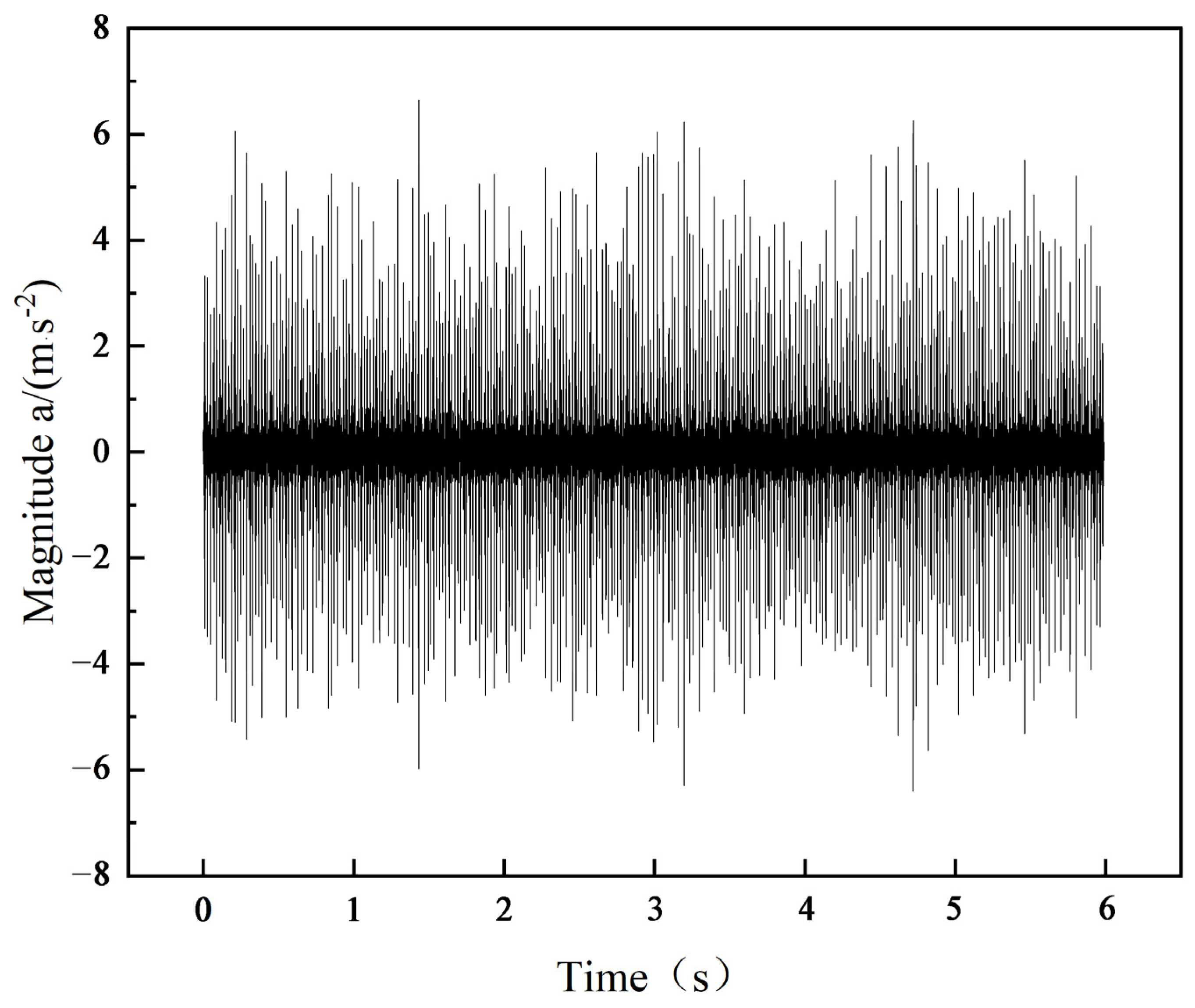
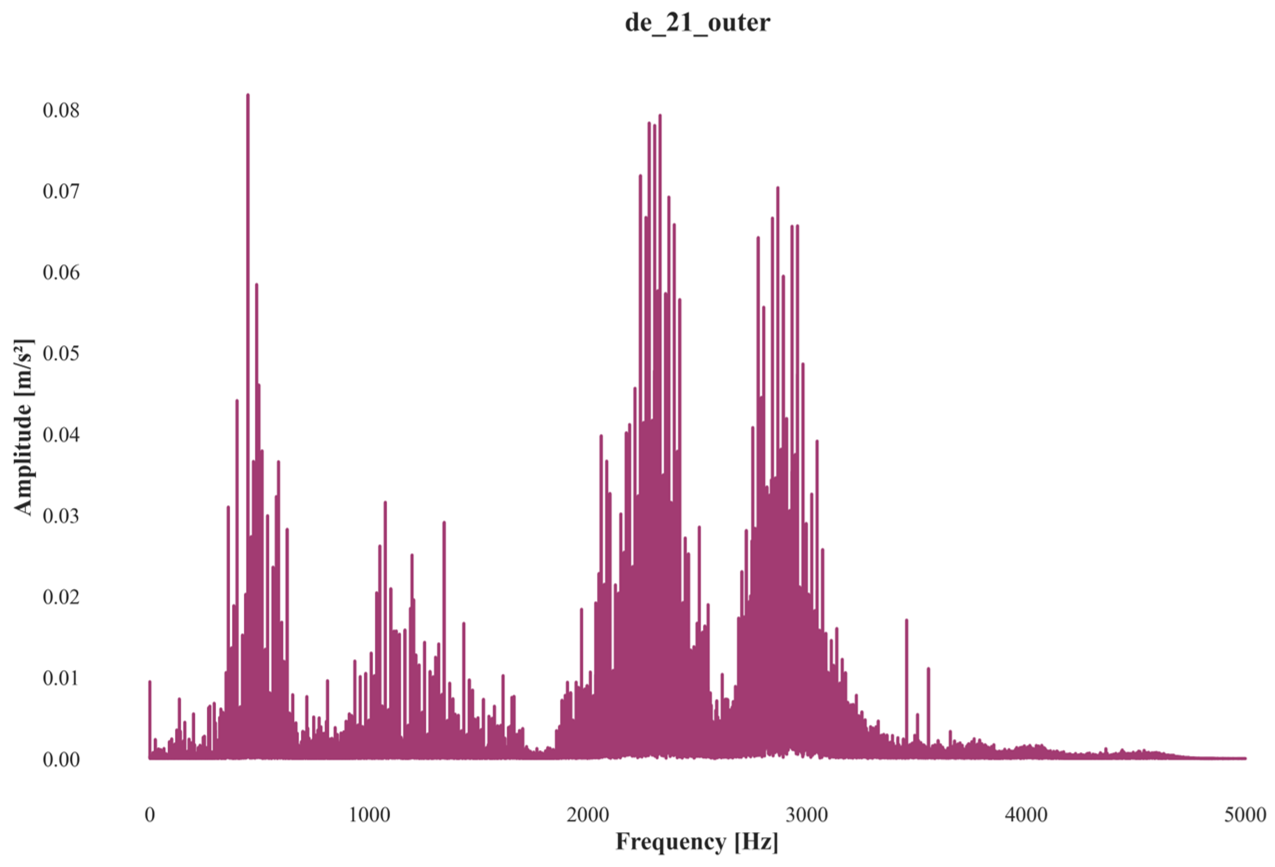
Taking the De_21_outer outer ring fault data as an example, the analysis begins with the original waveform of the rolling bearing outer ring fault signal, which exhibits significant noise. This noise obscures the impact signal, making it difficult to directly identify the frequency and period characteristics of the fault, as shown in Figure 9. In the corresponding spectrum, a prominent peak was observed in the 200–300 Hz frequency band, indicating that this band contains key fault characteristics. However, there was also substantial noise interference within the 0–100 Hz frequency range, which may lead to misjudgments, as depicted in Figure 10. These results highlight the need for further signal processing to extract clearer and more accurate fault characteristics.
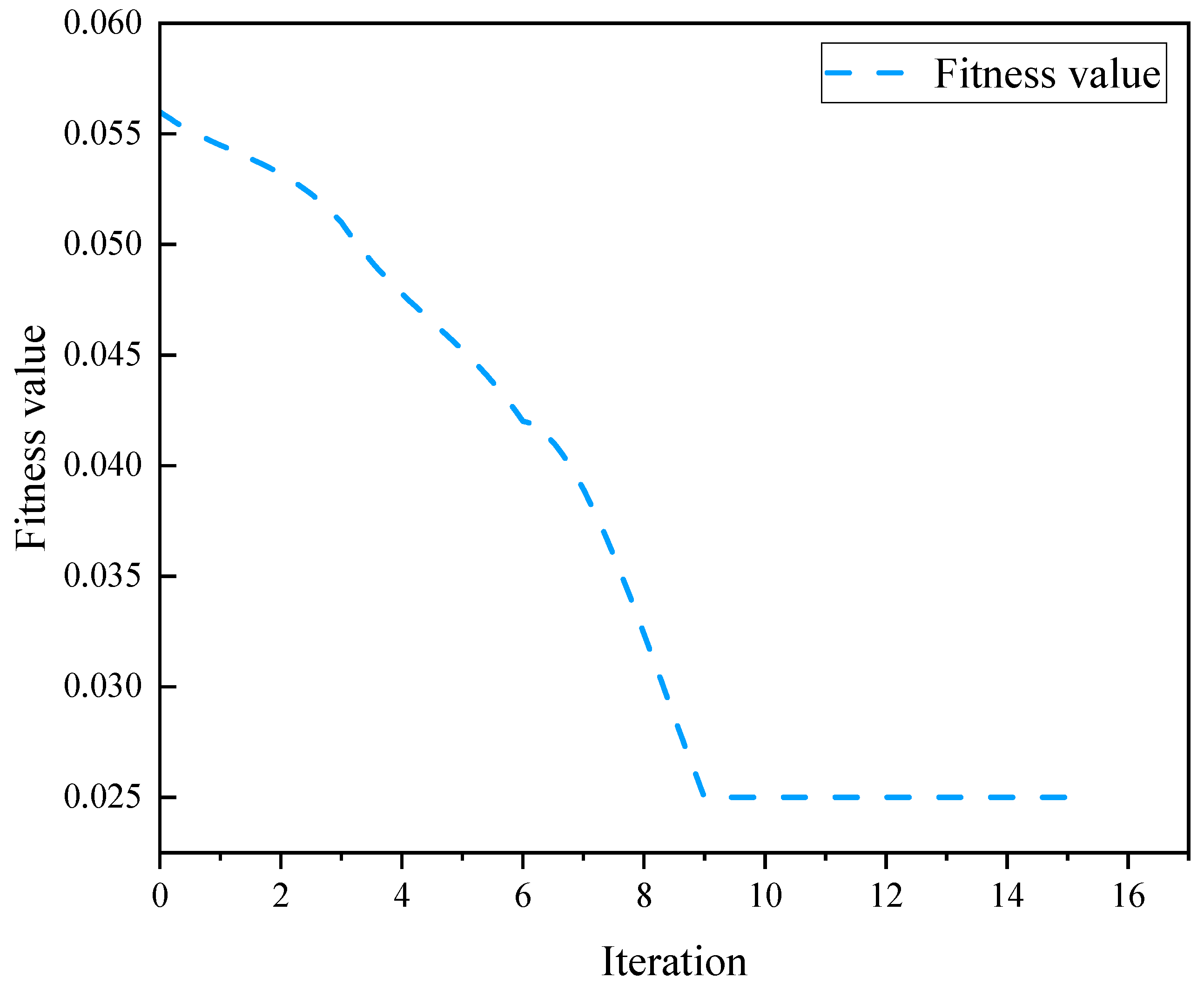
PSO was applied to optimize the Variational Mode Decomposition (VMD) process. After evolving for 9 generations, the optimization achieved a local minimum entropy value of 0.0257. The optimal function objective value corresponded to the parameters α = 4 and k = 1840, as shown in Figure 11. The entropy value serves as a measure of the information complexity following signal decomposition. A smaller entropy value typically indicated that the modes of the decomposed signal were more concentrated, thereby enhancing the distinguishability of the signal. The fitness function used in the PSO-VMD optimization process was a key indicator for assessing the quality of the solution. The objective of the fitness function was to minimize the entropy value, thereby achieving the optimal mode decomposition and improving the clarity of the extracted fault features.
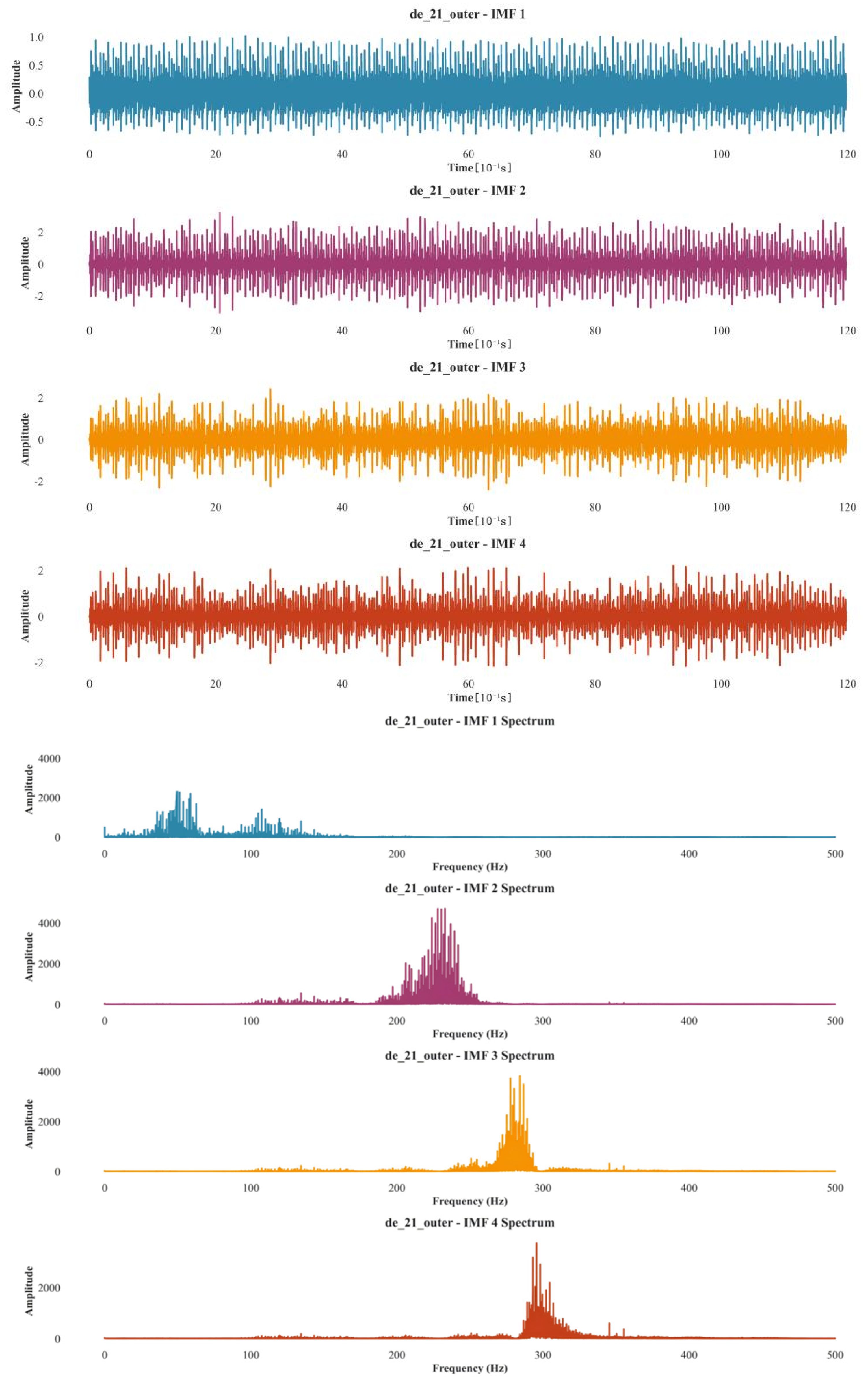
The original signal was processed using Variational Mode Decomposition (VMD) to obtain four modal function components along with their corresponding frequency domain representations. After applying PSO-VMD decomposition, the signal exhibited a peak between 200–300 Hz, which indicates the presence of a fault in the outer ring of the bearing. Additionally, the interference signal in the 0–100 Hz range was effectively suppressed. The PSO-VMD method demonstrates superior noise suppression, enhancing the clarity of the fault characteristics. The results were shown in Figure 12.
The Particle Swarm Optimization (PSO) algorithm was used to optimize the parameter combination [α, K] of Variational Mode Decomposition (VMD). The optimal solutions for each category, obtained through the optimization process, are presented in Table 3.
Taking a set of inner circle small fault data (De_7_inner) as an example, PSO, Random Forest (RF), and Genetic Algorithm (GA) were used to compare and analyze the parameter optimization results. In the optimization process, the cross-entropy loss function was adopted to assess the divergence between the predicted probability distribution output by the model and the true label distribution. Its mathematical expression was given as:
L = i = 1 N y i log ( y i ^ )
In the cross-entropy loss function, the value y i represents the one-hot encoding of the true category, and the value y ^ i corresponds to the probability distribution predicted by the model. As the cross-entropy loss decreases, it indicates that the model’s predicted probability distribution was getting closer to the true distribution, leading to improved classification accuracy. This reduction in loss directly correlates with the optimization algorithm’s better performance in correctly classifying the task, as the model’s predictions become more aligned with the actual class labels.
The PSO algorithm converged by the third iteration, achieving near-zero loss and outperforming the other two algorithms (Figure 13). The Random Forest (RF) algorithm, which relies on ensemble learning for feature selection and classification, does not perform as well in parameter optimization. Additionally, the Genetic Algorithm (GA) converges slowly, making it less efficient in this task. In conclusion, the PSO algorithm demonstrates superior optimization performance for this task, providing faster convergence and better classification accuracy. To further verify the effectiveness of the PSO-based signal decomposition, we compared PSO-VMD with the traditional FFT method. By analyzing the spectral clarity and modal separation results, as well as statistical indicators such as energy concentration and kurtosis, we demonstrated that PSO-VMD can more effectively isolate informative signal components, which significantly enhances the downstream feature extraction and classification performance.
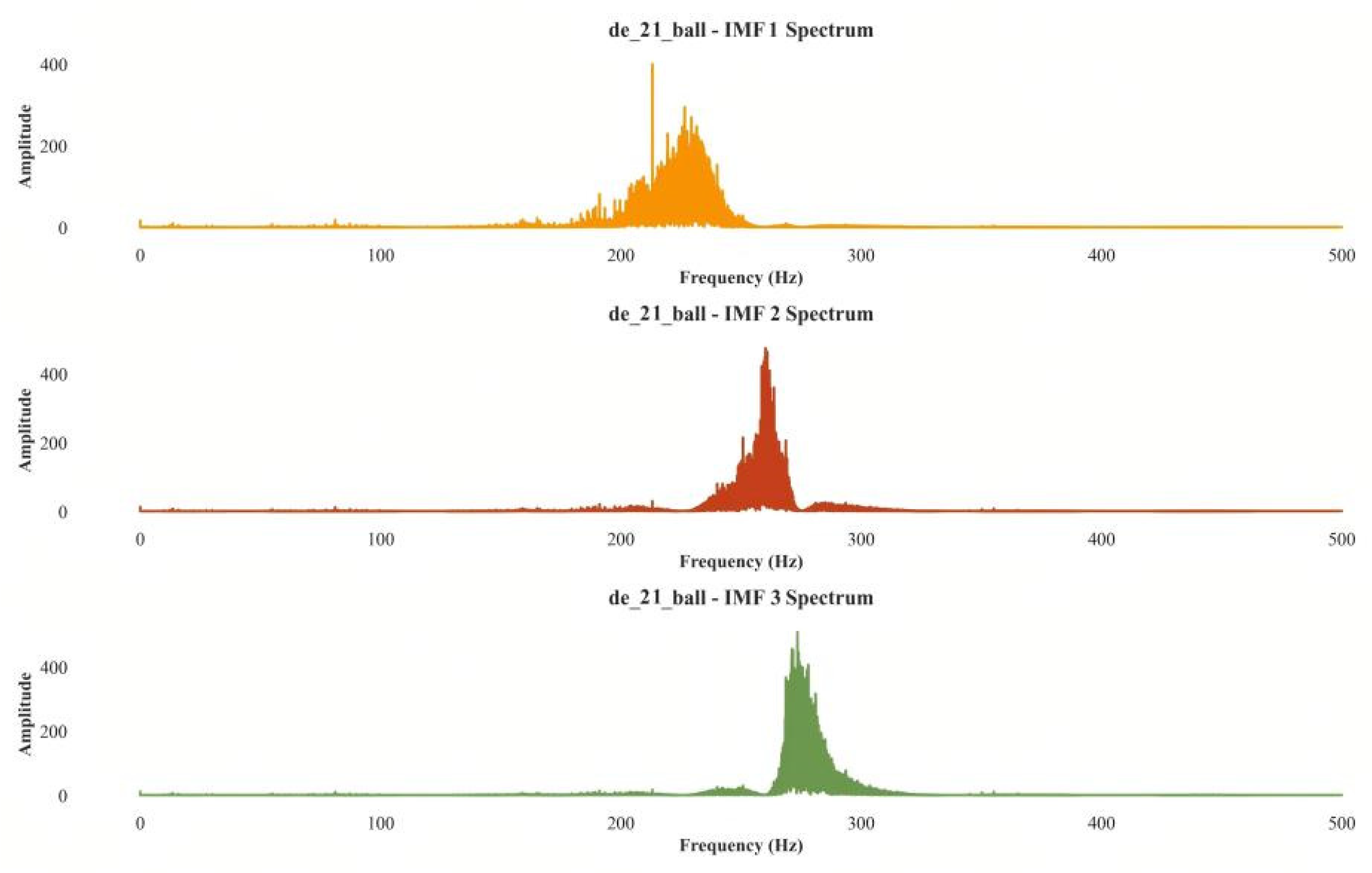
To further verify the effectiveness of PSO-VMD feature extraction, the rolling element (De_21_ball) fault was used as an example. The bearing vibration signal was decomposed using EMD, VMD, and PSO-VMD methods. After EMD decomposition, the energy was predominantly concentrated in the first few components, so the first three modal components were selected for analysis. The spectrum of the modal components obtained after EMD decomposition reveals significant modal aliasing between 200 Hz and 300 Hz, as shown in Figure 14. This modal aliasing can obscure the fault characteristics, making it difficult to distinguish between different modes and accurately identify the fault. It should be noted that the initial loss value may appear slightly below zero due to the inclusion of bias initialization and L2 regularization terms, which do not affect the non-negativity of the primary loss function (e.g., cross-entropy).
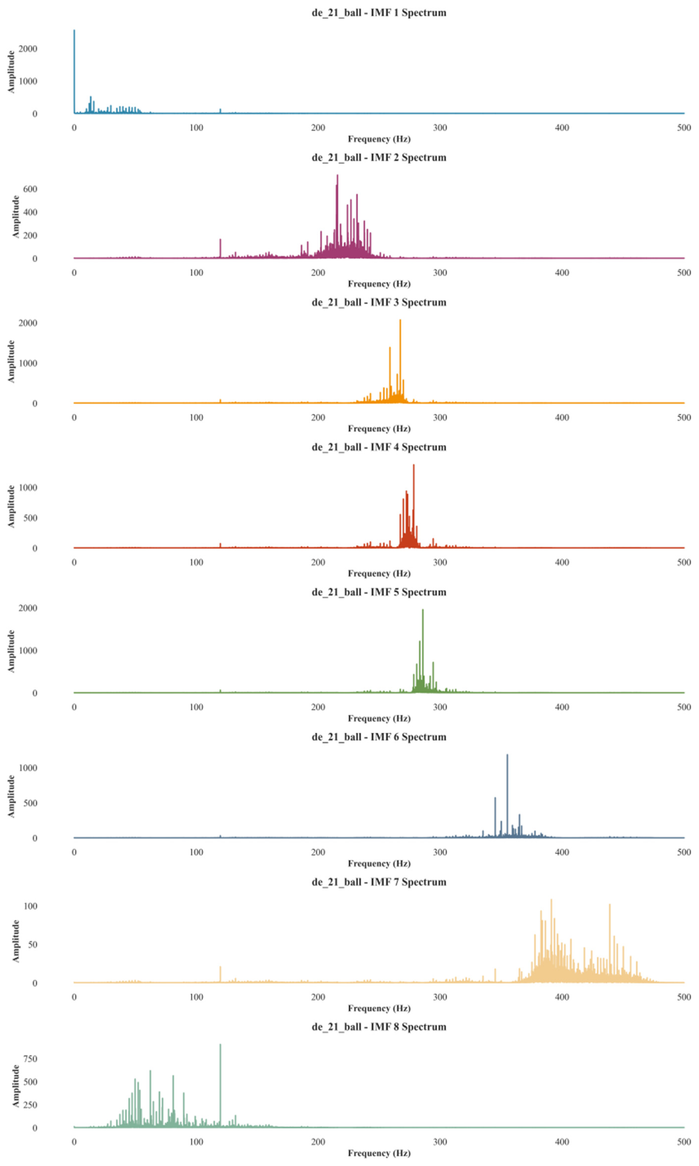
The spectrum of the modal components obtained after signal decomposition using the VMD method showed that the modal components are concentrated around their respective center frequencies, effectively reducing the modal aliasing phenomenon. However, due to the manual selection of the K value and penalty factor α, some modal aliasing still persists. Specifically, aliasing was observed in the modal components IMF = 3, IMF = 4, and IMF = 5, with frequencies ranging between 200–300 Hz and amplitudes between 0–1000. As shown in Figure 15. Despite the reduction in aliasing compared to EMD, the optimization of these parameters remains crucial to further mitigate the aliasing effect.
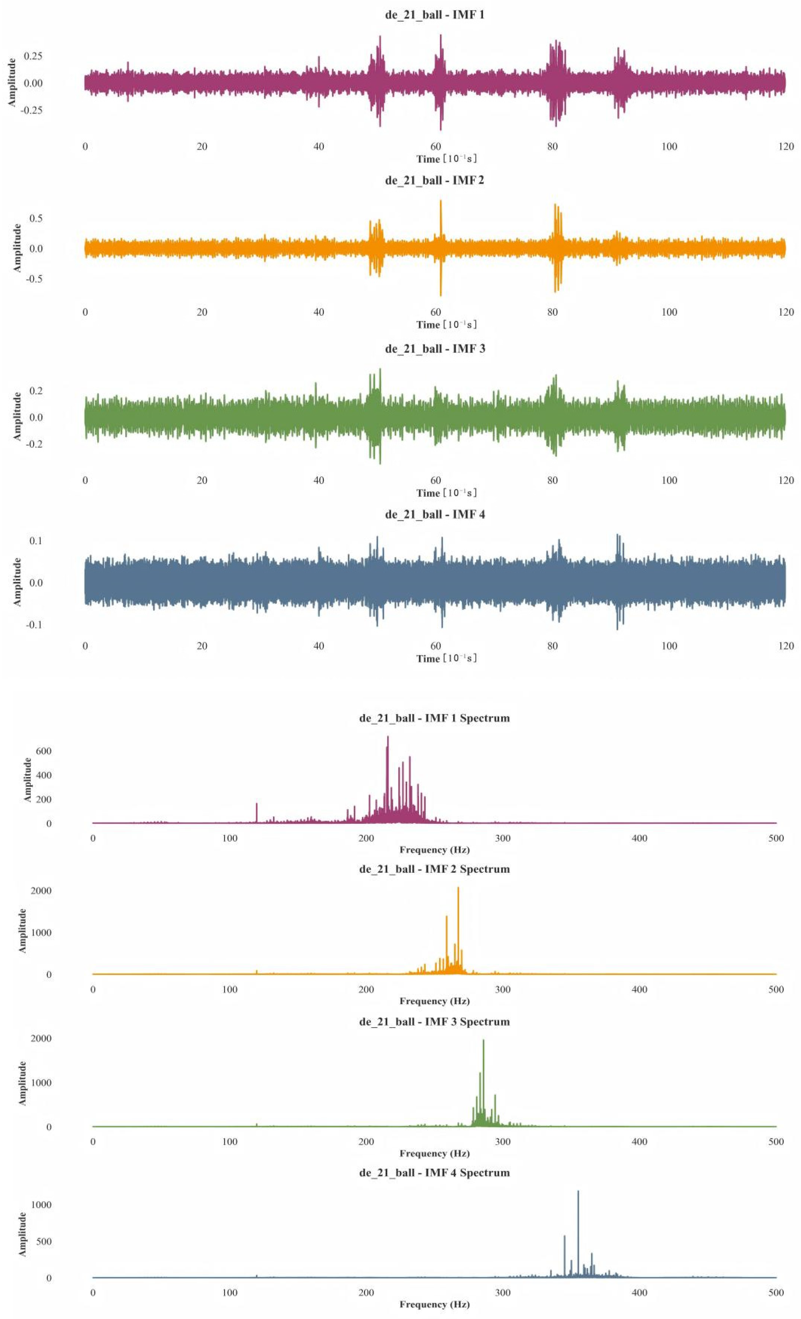
The optimal parameter combination obtained through PSO optimization of VMD was [4, 1248]. This parameter combination was applied to VMD to decompose the post-fault vibration signal within the time range of 0 to 1.2 s. The decomposition resulted in four Intrinsic Mode Function (IMF) components, each with its corresponding spectrum diagram. Unlike other methods, the PSO-VMD decomposition method does not exhibit frequency aliasing, ensuring that the spectral components remain distinct and non-interfering. By optimizing the parameters, PSO-VMD achieves a reasonable decomposition of the original signal, effectively separating different modal components. This method demonstrates excellent adaptability in fault signal processing. Each IMF component exhibits a clear and well-defined spectral distribution in the frequency domain, facilitating more accurate feature extraction and fault diagnosis. which leads to more accurate feature extraction and diagnosis of faults. Results are shown in Figure 16.

3.2. TCB Model Structure Proposed in This Paper

To assess the contribution of each component within the proposed model, this paper conducts an ablation study. In this experiment, the Transformer, BiGRU, and CNN modules are individually excluded to create different model variants, and their performance is then compared. The results of these ablation tests are summarized in Table 4, enabling a clear evaluation of the role and impact of each module on the model’s overall effectiveness. All results are obtained under the unified preprocessing and training regime described in Section 2.2 and Section 3.1; PSO–VMD features are provided to every baseline.
CNN Model: Using only the CNN module, the model achieves an accuracy of 93.4%. However, CNN was limited to capturing local features and struggles with handling long-range dependencies, resulting in suboptimal performance when processing time series data.
CNN-Transformer Model: By combining the CNN and Transformer modules, the model’s accuracy improves to 95.3%. The Transformer module enhances the model’s ability to capture long-range dependencies through the self-attention mechanism, significantly boosting classification performance.
CNN-BiGRU Model: When the CNN and BiGRU modules were combined, the model’s accuracy also reaches 95.2%. The BiGRU module enhances the model’s ability to capture temporal patterns via bidirectional modeling. However, the absence of the Transformer module limits the model’s performance when processing long sequences.
CNN-Transformer-BiGRU Model: Combining all three modules-CNN, Transformer, and BiGRU-the model achieves the highest accuracy of 97.1%. The synergy of these modules allows the model to simultaneously capture local features, long-range dependencies, and time series information, leading to a significant improvement in fault diagnosis accuracy.
Through these four sets of ablation experiments, it is clear that the Transformer, BiGRU, and CNN modules in the Transformer-CNN-BiGRU model each play an essential role in classification. The model’s accuracy of 97% in the combined module configuration represents the optimal result across all experiments, confirming the effectiveness of using multiple modules together. This combination allowed the model to more effectively capture the characteristics of the data during the training process.
To further verify the rationality of the parameter settings in the proposed optimization algorithm, we conducted an ablation study on two key hyperparameters: swarm size and the number of iterations. As shown in Table 5 and Table 6, the model achieves the best balance between performance and computational cost when the swarm size is set to 30 and the number of iterations is set to 50. These results confirm the effectiveness and efficiency of the selected configuration.
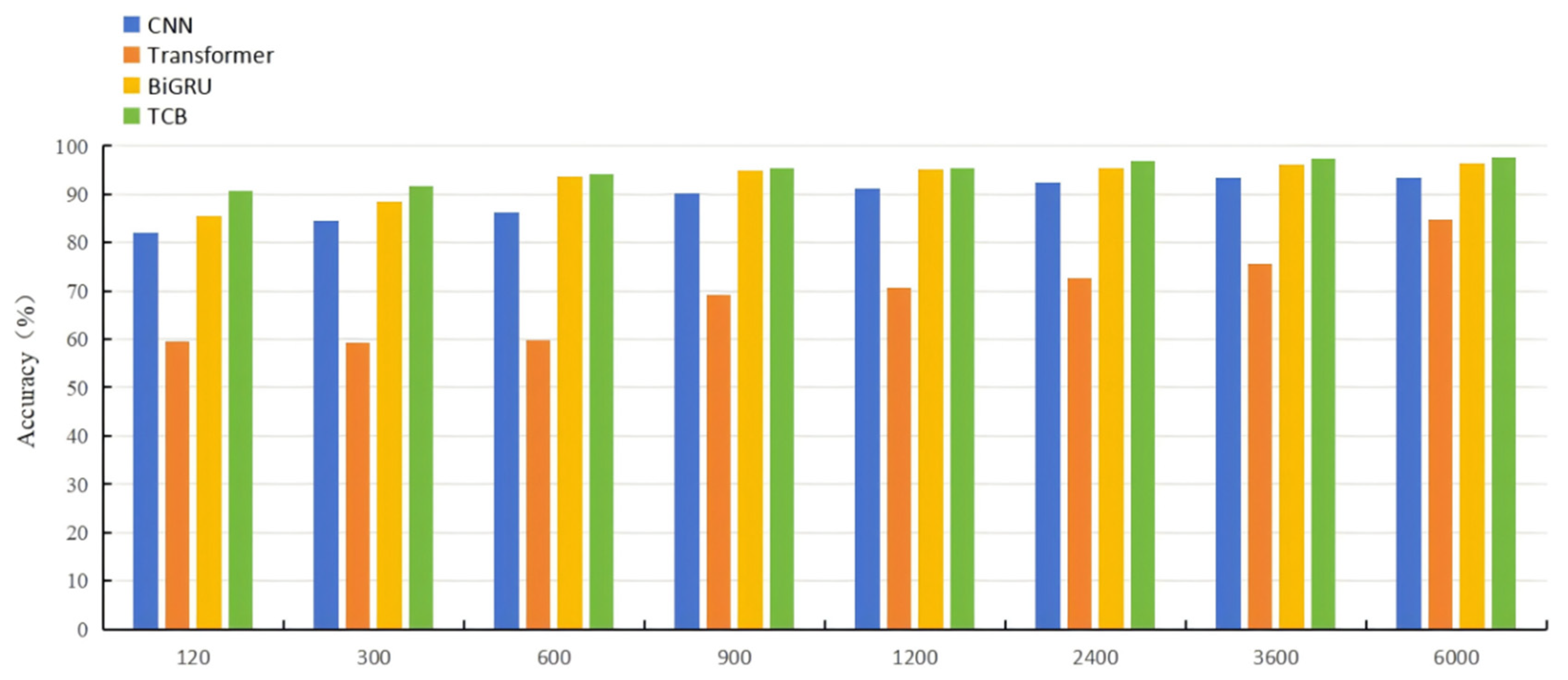
To further verify the important role of each module, individual CNN, Transformer, and BiGRU modules were trained with different sample sizes to analyze their specific contributions. The original experimental data was constructed using a 12 kHz dataset, with an additional dataset created for a load of 0. First, the original sample was divided into a training set, a validation set, and a test set with a ratio of 6:2:2. A one-dimensional sample with a length of 1024 was extracted from each part of the original sample and processed through a sliding window. Each one-dimensional sample was then converted into a training sample, a validation sample, and a test sample for the model using a short-time Fourier transform (STFT). The dataset consists of 6000 training samples, 2000 validation samples, and 2000 test samples, totaling 10,000 samples. For training, different numbers of training samples were selected, with training integration ratios of 120, 300, 600, 900, 1200, 2400, 3600, and 6000 training samples. The time taken for each training scenario was recorded, allowing for an evaluation of the performance and efficiency of each module as the sample size varied. This experiment helps highlight the impact of sample size on training time and model performance, providing further insight into the role of each module in the overall system.
With the increase in training sample size, the accuracy of all models showed a steady improvement before reaching a plateau. Specifically, for the Transformer model, when the number of training samples was below 1200, its accuracy reaches a maximum of 69.16%. However, when the number of training samples reaches 6000, the accuracy increases to 84.82%. These results suggest that the Transformer model required a large amount of data to perform well and struggles to capturing local, subtle information effectively. The CNN model, on the other hand, achieves an accuracy greater than 90% with smaller sample sizes (fewer than 1200 samples), and stabilizes at an accuracy of 93.4% with 3600 samples. This indicates that CNN has high computational efficiency and can perform well with smaller datasets, but its ability to process more complex signals was limited compared to the other models. The BiGRU model demonstrates the highest accuracy among the single models across eight training scenarios with varying sample sizes, as shown in Figure 17. However, since BiGRU considers both forward and backward time information, and calculates the state of each time step iteratively, it was computationally slower than the CNN and Transformer models. The longest running time recorded for BiGRU was 101.7 s, as shown in Table 7. In summary, while the Transformer model requires more data to achieve higher accuracy, CNN was efficient for smaller datasets but may struggle with complex signals. BiGRU outperforms both models in accuracy but at the cost of longer training times.
By combining CNN, BiGRU, and Transformer, a complementary structure was formed that integrates local feature extraction, short time series modeling, and global information modeling. This combined model achieves an accuracy of over 97% in the ablation experiment. In the test with 6000 training samples, the proposed model achieves the best performance in terms of both time and test accuracy, as shown in Table 7. Furthermore, the original data was fed into the model after PSO-VMD feature extraction. After 18 iterations of training (where one epoch refers to a complete forward and backward pass through the entire training dataset), the model reaches stability and gradually converges, with the loss value approaching 0. As shown in Figure 18, the model reaches an accuracy of 98.9%. as shown in Figure 18. The results demonstrate that the model structure and feature extraction method proposed in this paper significantly enhance the performance of fault diagnosis, effectively enhancing both the accuracy and efficiency of the system.
To evaluate the stability and robustness of the proposed model, five independent experiments were conducted with randomized training-validation splits. The results demonstrated consistent performance across different splits, with an average accuracy of 98.8% ± 0.1%, precision of 98.6% ± 0.1%, recall of 99.2% ± 0.1%, and F1-score of 98.9% ± 0.1%. The detailed results are presented in Table 8, which confirm the strong generalization ability and reliability of the proposed model. The p-values obtained from t-tests against baseline models were all < 0.05, confirming that the performance improvements are statistically significant. All results are averaged over five runs (mean ± std) with 95% confidence intervals computed from two-sided t intervals. Statistical significance vs. baselines is assessed using two-sided t-tests, and Cohen’s d is reported as the effect size.
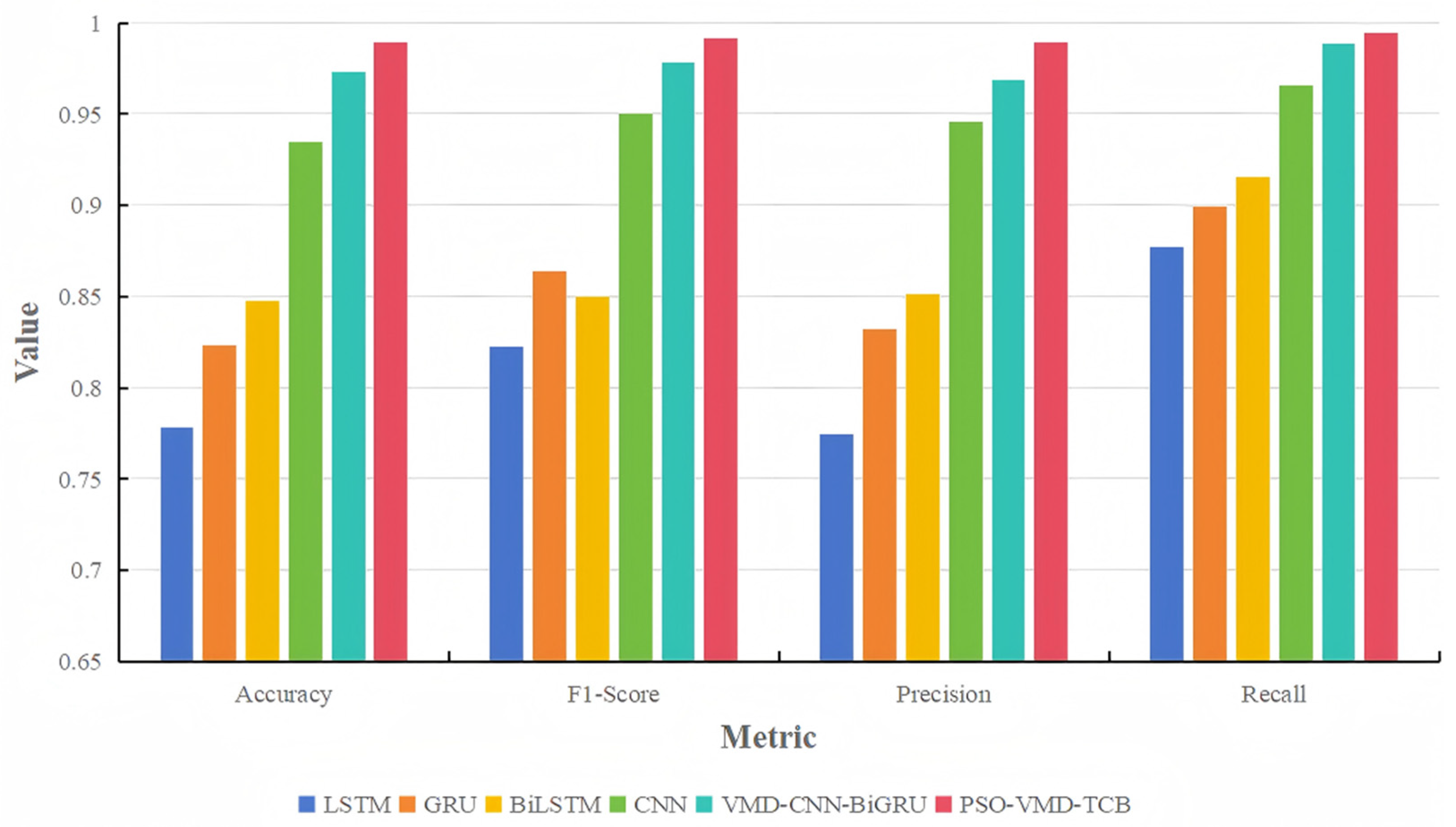
In order to further verify the comprehensive performance of this model, the dataset processed by PSO-VMD was used to compare the performance of five deep learning models, CNN, LSTM, BiLSTM, GRU, VMD-CNN-BiGRU and the VMD-TCB model proposed herein. The comparison considers metrics such as accuracy. precision, recall, and F1 score during the training process, as shown in Figure 19.
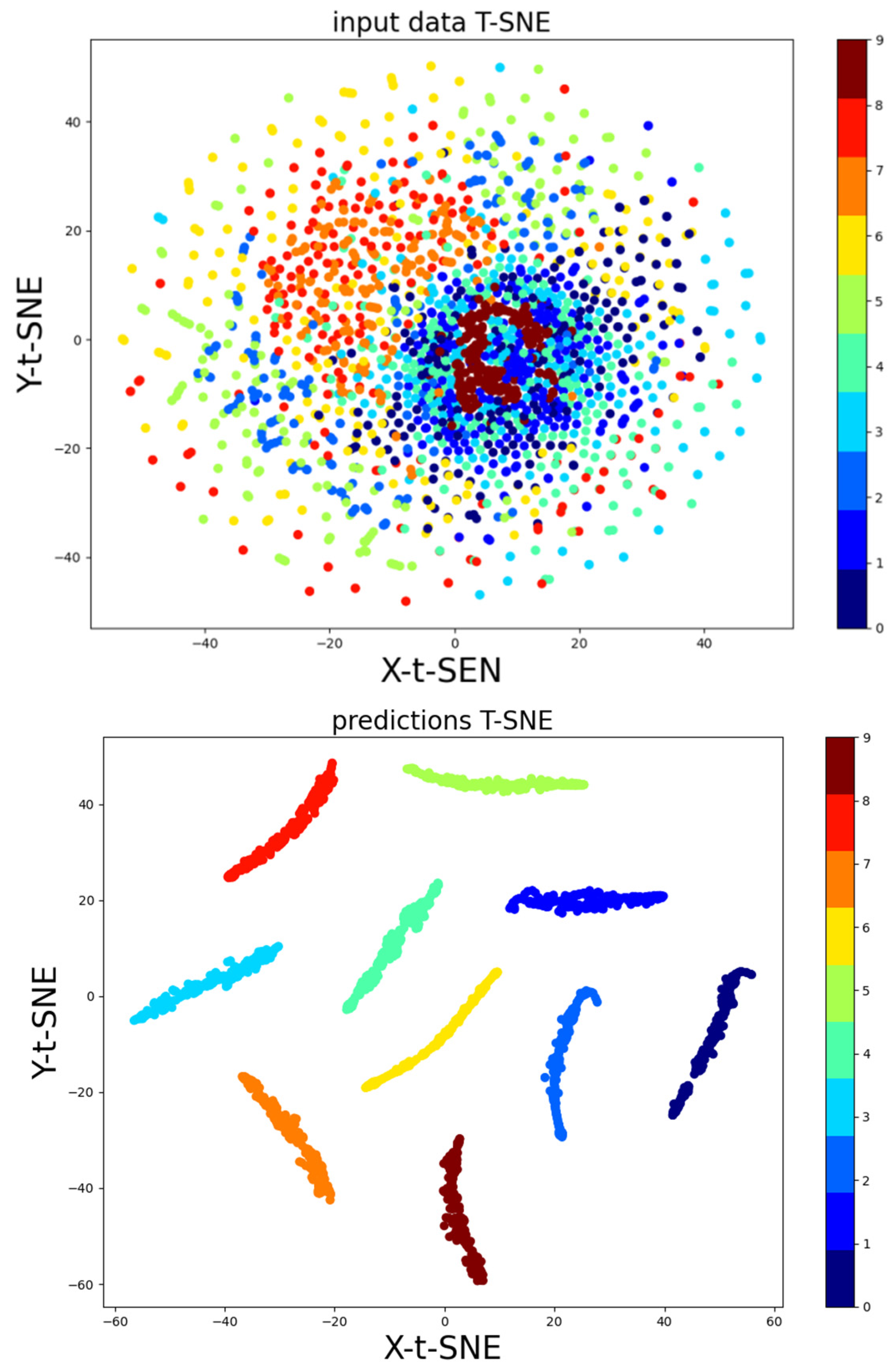
To assess the errors in the experimental results of the PSO-VMD-TCB model, this paper presents a confusion matrix and t-SNE visualization. The diagonal elements of the confusion matrix correspond to the number of correctly classified samples, while the off-diagonal elements represent misclassified samples. These values provided valuable insight into the model’s performance across different fault types and highlight areas of misclassification, as shown in Figure 20, For the 10-class task we additionally report macro averages derived from the confusion matrix: Macro-Precision/Recall/F1 = 0.9768/0.9765/0.9766. Additionally, the t-SNE visualization was used to differentiate fault types, with each fault type marked by a distinct color. This allows for identification of patterns and clusters within the feature space. By combining these analyses, a more comprehensive understanding of the model’s classification performance was achieved, demonstrating its effectiveness in distinguishing between various fault categories.
This paper compares the performance of the proposed method with other bearing fault diagnosis methods that have been studied on the CWRU bearing dataset. For the de_14_ball dataset, the model correctly classifies 2109 samples, with only 34 samples misclassified as de_14_outer, just 1.6% of misclassification.In reference [22], the overall classification accuracy is 95.2%, showing relatively limited performance in distinguishing some fault categories. In contrast, the proposed model achieves 98.9% accuracy, significantly improving the recognition capability and reducing class confusion. In reference [23], the probability of correct prediction for category 14 is 75%, with 22% misclassified as category 6. In reference [24], the misclassification rate is much higher, with category 2 misclassified as category 3 at a rate of 37%, and 11% misclassified as category 1, resulting in an overall misclassification rate of 48%. The model proposed in this paper achieves the lowest classification error ratio, with only 7.1% misclassification across all categories, demonstrating superior performance in bearing fault diagnosis.
In literature [24], there remains a noticeable overlap between the real data (red) and the generated data (blue), and the features of different classifications were quite similar. This overlap makes it challenging to confidently distinguish between categories. In contrast, in this paper, the data points form distinct, well-separated clusters in the low-dimensional space. This clear separation enhances the discriminative ability of the model, significantly improving classification quality, as illustrated in Figure 21. The results highlight the superior effectiveness of the proposed method in distinguishing between fault types, demonstrating its improved performance relative to prior approaches.
Finally, this paper provides a summary of the publication years for each method, offering a comprehensive overview of recent advancements in the field. In the context of the CWRU dataset, various researchers have employed different optimization strategies to enhance neural network performance and improve feature extraction techniques, thereby advancing traditional neural network methodologies. In contrast, the PSO-VMD-TCB method proposed in this paper demonstrates superior performance, achieving higher accuracy in processing the CWRU dataset. The comparison results, as presented in Table 9, underscore the effectiveness of the proposed approach relative to existing methods in the literature. These results also demonstrate a symmetric trade-off among diagnostic accuracy, convergence speed, and computational efficiency, highlighting the balanced nature of the proposed framework.

4. Conclusions

This paper presents a bearing fault diagnosis approach that couples PSO-VMD feature extraction with a TCB model. The main conclusions are as follows:
On the publicly available CWRU dataset, the proposed method achieved 98.9% accuracy, 98.8% precision, 99.4% recall, and 99.1% F1-score, outperforming existing mainstream comparison models. The model converged stably at the 18th epoch with a 29.2 s inference time, making it 13.4% faster than the ICEEMDAN-WTATD-DaSqueezeNet model. Ablation studies confirmed that integrating the Transformer, CNN, and BiGRU modules significantly improved accuracy, 4.3% improvement over CNN, and 14.4% improvement over Transformer. In conclusion, the proposed method not only exhibits excellent diagnostic performance but also demonstrates fast convergence and adaptability for deployment, offering an innovative solution for intelligent fault detection in industrial applications.
Despite its promising results, the study has certain limitations. The model’s performance partially relies on optimized hyperparameters, which may require re-tuning under different datasets or operating conditions. Furthermore, the model has not yet been validated under multiple loads, high noise levels, or in real industrial scenarios, which limits its generalizability in practical environments.
Future work will focus on introducing adaptive or lightweight attention mechanisms to further reduce computational costs. Additionally, more diverse and noisy datasets will be used to evaluate the model’s robustness. Finally, we plan to deploy the model on edge computing devices or embedded platforms to promote its real-time application in industrial settings.
Overall, the PSO-VMD-TCB framework exemplifies how symmetry and balanced design principles can inspire intelligent fault detection models with enhanced robustness and generalization.

Author Contributions

Conceptualization, H.D.; investigation, G.L. and L.Z.; funding acquisition, H.D.; methodology, D.Y.; validation, D.Y. and G.L.; writing original draft, D.Y.; supervision, H.D.; project administration, L.Z.; writing-review and editing, D.Y.; data curation, G.L. and L.Z.; formal analysis, G.L.; resources, D.Y. All authors have read and agreed to the published version of the manuscript.

Funding

This work was supported by Tianjin Municipal Science and Technology Commission Planned Project [grant number 2011Z0189] and Tianjin Science and Technology Commission Enterprise Science and Technology Commissioner’s Project [grant number 22YDTPJC00670].

Data Availability Statement

The original contributions presented in this study are included in the article. Further inquiries can be directed to the corresponding author.

Conflicts of Interest

Author Liying Zhang was employed by the company Hangzhou Zhihui Jiang Switchgear Co., Ltd. The remaining authors declare that the research was conducted in the absence of any commercial or financial relationships that could be construed as a potential conflict of interest.

References

  1. Gao, Q.W.; Liu, W.Y.; Tang, B.P.; Li, G.J. A novel wind turbine fault diagnosis method based on intergral extension load mean decomposition multiscale entropy and least squares support vector machine. Renew. Energy 2018, 116, 169–175. [Google Scholar] [CrossRef]
  2. Prabhakar, S.; Mohanty, A.R.; Sekhar, A.S. Application of discrete wavelet transform for detection of ball bearing race faults. Tribol. Int. 2002, 35, 793–800. [Google Scholar] [CrossRef]
  3. Hoang, D.T.; Kang, H.J. A survey on Deep Learning based bearing fault diagnosis. Neurocomputing 2019, 335, 327–335. [Google Scholar] [CrossRef]
  4. Zhao, Z.B.; Li, T.F.; Wu, J.Y.; Sun, C.; Wang, S.B.; Yan, R.Q.; Chen, X.F. Deep learning algorithms for rotating machinery intelligent diagnosis: An open source benchmark study. Isa Trans. 2020, 107, 224–255. [Google Scholar] [CrossRef]
  5. An, B.T.; Zhao, Z.B.; Wang, S.B.; Chen, S.W.; Chen, X.F. Sparsity-assisted bearing fault diagnosis using multiscale period group lasso. Isa Trans. 2020, 98, 338–348. [Google Scholar] [CrossRef]
  6. Dong, H.B.; Qi, K.Y.; Chen, X.F.; Zi, Y.Y.; He, Z.J.; Li, B. Sifting process of EMD and its application in rolling element bearing fault diagnosis. J. Mech. Sci. Technol. 2009, 23, 2000–2007. [Google Scholar] [CrossRef]
  7. Zou, P.; Hou, B.C.; Jiang, L.; Zhang, Z.J. Bearing Fault Diagnosis Method Based on EEMD and LSTM. Int. J. Comput. Commun. Control 2020, 15, 1–14. [Google Scholar] [CrossRef]
  8. Ding, J.K.; Huang, L.P.; Xiao, D.M.; Li, X.J. GMPSO-VMD Algorithm and Its Application to Rolling Bearing Fault Feature Extraction. Sensors 2020, 20, 1946. [Google Scholar] [CrossRef]
  9. Song, X.M.; Wei, W.H.; Zhou, J.B.; Ji, G.J.; Hussain, G.; Xiao, M.H.; Geng, G.S. Bayesian-Optimized Hybrid Kernel SVM for Rolling Bearing Fault Diagnosis. Sensors 2023, 23, 5137. [Google Scholar] [CrossRef]
  10. Zhou, J.B.; Xiao, M.H.; Niu, Y.; Ji, G.J. Rolling Bearing Fault Diagnosis Based on WGWOA-VMD-SVM. Sensors 2022, 22, 6281. [Google Scholar] [CrossRef]
  11. Wang, B.; Qiu, W.T.; Hu, X.; Wang, W. A rolling bearing fault diagnosis technique based on fined-grained multi-scale symbolic entropy and whale optimization algorithm-MSVM. Nonlinear Dyn. 2024, 112, 4435–4447. [Google Scholar] [CrossRef]
  12. Shao, X.R.; Kim, C.S. Unsupervised Domain Adaptive 1D-CNN for Fault Diagnosis of Bearing. Sensors 2022, 22, 4156. [Google Scholar] [CrossRef] [PubMed]
  13. Chen, X.H.; Yang, R.; Xue, Y.H.; Huang, M.J.; Ferrero, R.; Wang, Z.D. Deep Transfer Learning for Bearing Fault Diagnosis: A Systematic Review Since 2016. IEEE Trans. Instrum. Meas. 2023, 72, 3508221. [Google Scholar] [CrossRef]
  14. Liu, X.; Wu, R.Q.; Wang, R.G.; Zhou, F.; Chen, Z.F.; Guo, N.H. Bearing fault diagnosis based on particle swarm optimization fusion convolutional neural network. Front. Neurorobotics 2022, 16, 1044965. [Google Scholar] [CrossRef]
  15. Yan, X.; Jin, X.P.; Jiang, D.; Xiang, L. Remaining useful life prediction of rolling bearings based on CNN-GRU-MSA with multi-channel feature fusion. Nondestruct. Test. Eval. 2024, 1–26. [Google Scholar] [CrossRef]
  16. Xu, Z.W.; Li, Y.F.; Huang, H.Z.; Deng, Z.M.; Huang, Z.X. A novel method based on CNN-BiGRU and AM model for bearing fault diagnosis. J. Mech. Sci. Technol. 2024, 38, 3361–3369. [Google Scholar] [CrossRef]
  17. An, Y.Y.; Zhang, K.; Liu, Q.; Chai, Y.; Huang, X.H. Rolling Bearing Fault Diagnosis Method Base on Periodic Sparse Attention and LSTM. IEEE Sens. J. 2022, 22, 12044–12053. [Google Scholar] [CrossRef]
  18. Yang, Z.H.; Cen, J.; Liu, X.; Xiong, J.N.; Chen, H.H. Research on bearing fault diagnosis method based on transformer neural network. Meas. Sci. Technol. 2022, 33, 085111. [Google Scholar] [CrossRef]
  19. Zhou, A.Y.; Farimani, A.B. FaultFormer: Pretraining Transformers for Adaptable Bearing Fault Classification. IEEE Access 2024, 12, 70719–70728. [Google Scholar] [CrossRef]
  20. Dragomiretskiy, K.; Zosso, D. Variational Mode Decomposition. IEEE Trans. Signal Process. 2014, 62, 531–544. [Google Scholar] [CrossRef]
  21. Lecun, Y.; Bottou, L.; Bengio, Y.; Haffner, P. Gradient-based learning applied to document recognition. Proc. IEEE 1998, 86, 2278–2324. [Google Scholar] [CrossRef]
  22. Liang, B.; Feng, W.W. Bearing Fault Diagnosis Based on ICEEMDAN Deep Learning Network. Processes 2023, 11, 2440. [Google Scholar] [CrossRef]
  23. Geng, Z.; Yuan, K.; Ma, B.; Han, Y. Rolling Bearing Fault Diagnosis based on ICEEMDAN-WTATD-DaSqueezeNet. In Proceedings of the 2023 IEEE 12th Data Driven Control and Learning Systems Conference (DDCLS), Xiangtan, China, 12–14 May 2023; pp. 1510–1515. [Google Scholar]
  24. Bai, G.L.; Sun, W.; Cao, C.; Wang, D.F.; Sun, Q.C.; Sun, L. GAN-Based Bearing Fault Diagnosis Method for Short and Imbalanced Vibration Signal. IEEE Sens. J. 2024, 24, 1894–1904. [Google Scholar] [CrossRef]
  25. Wang, Y.; Li, D.X.; Li, L.; Sun, R.D.; Wang, S.Q. A novel deep learning framework for rolling bearing fault diagnosis enhancement using VAE-augmented CNN model. Heliyon 2024, 10, e35407. [Google Scholar] [CrossRef] [PubMed]
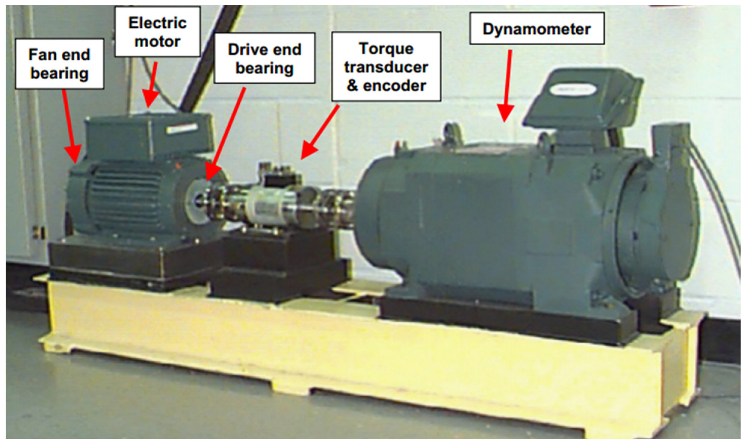
Figure 1. CWRU bearing test bench.
Symmetry 17 01780 g001
Figure 2. PSO algorithm flow.
Symmetry 17 01780 g002
Figure 3. PSO-VMD parameter optimization process.
Symmetry 17 01780 g003
Figure 4. Bearing fault diagnosis process.
Symmetry 17 01780 g004
Figure 5. Transformer encoder-decoder structure diagram.
Symmetry 17 01780 g005
Figure 6. Schematic diagram of CNN model.
Symmetry 17 01780 g006
Figure 7. Structural diagram of BiGRU.
Symmetry 17 01780 g007
Figure 8. Model structure diagram.
Symmetry 17 01780 g008
Figure 9. Outer ring fault signal waveform.
Symmetry 17 01780 g009
Figure 10. Spectrum of outer race fault signal. Note: The amplitude difference between Figure 9 and Figure 10 is due to the lack of consistent FFT normalization. Figure 9 shows the unnormalized FFT of the raw signal, while Figure 10 presents the magnitude without dividing by the sampling length N. Since the analysis focuses on frequency distribution rather than absolute magnitude, this discrepancy does not affect the interpretation.
Symmetry 17 01780 g010
Figure 11. Fitness value changing with the number of iterations.
Symmetry 17 01780 g011
Figure 12. The size of the IMF after the improvement.
Symmetry 17 01780 g012
Figure 13. PSO-VMD parameter optimization comparison.
Symmetry 17 01780 g013
Figure 14. EMD spectrum.
Symmetry 17 01780 g014
Figure 15. VMD spectrum.
Symmetry 17 01780 g015
Figure 16. PSO-VMD time domain and frequency domain diagrams.
Symmetry 17 01780 g016
Figure 17. Average diagnostic accuracy of different fault diagnosis methods.
Symmetry 17 01780 g017
Figure 18. Accuracy line graph and loss rate line graph.
Symmetry 17 01780 g018
Figure 19. Comparison of various models.
Symmetry 17 01780 g019
Figure 20. PSO-VMD-TCB confusion matrix.
Symmetry 17 01780 g020
Figure 21. t-SNE bearing fault diagnosis 10 classification before and after comparison.
Symmetry 17 01780 g021
Table 1. Drive end bearing data.
Serial NumberFault LocationDamage Size (Inches)Speed
(r/min)
Load
(N)
1Normal017970
2Outer0.00717970
3Outer0.01417970
4Outer0.02117970
5Inner0.00717970
6Inner0.01417970
7Inner0.02117970
8Ball0.00717970
9Ball0.01417970
10Ball0.02117970
Table 2. Parameter settings of CNN-BiGRU model.
Parameter NameParameter Settings
Convolutional LayerNumber of convolution kernels: 32 Convolution kernel size: 3
BiGRU LayerThe number of hidden units is 32
Fully connected layerNumber of neurons: 10
Table 3. PSO-VMD parameter optimization results.
PSO Parameter Optimization ClassificationDecomposition Number
K
Penalty Factor
α
De_normal61000
De_7_inner51168
De_7_ball61254
De_7_outer61168
De_14_inner41345
De_14_ball41548
De_14_outer61257
De_21_inner41766
De_21_ball41248
De_21_outer41840
Table 4. Accuracy of different module fusions on the dataset.
MethodAccuracy (%)
CNN93.4
CNN-Transformer95.3
CNN-BiGRU95.2
CNN-Transformer-BiGRU97.1
Table 5. Effect of swarm size on model performance.
Swarm SizeAccuracy (%)Precision (%)Recall (%)F1-Score (%)
1098.398.098.998.4
2098.698.499.098.7
3098.898.699.298.9
4098.898.599.198.8
5098.798.499.098.7
Table 6. Impact of maximum number of iterations on model performance.
IterationsAccuracy (%)Precision (%)Recall (%)F1-Score (%)
1098.498.198.998.5
3098.698.399.098.7
5098.898.699.298.9
7098.898.599.298.8
10098.798.599.198.7
Table 7. Performance results of each model.
ModelBest AccuracyTime
CNN93.4%75.3 s
Transformer84.8%83.1 s
BiGRU96.3%101.7 s
TCB97.6%29.2 s
Table 8. Performance evaluation metrics of the TCB model under different random splits.
RunAccuracy (%)Precision (%)Recall (%)F1-Score (%)
198.698.499.298.8
298.998.899.399.0
398.798.699.198.9
498.898.799.499.0
598.898.599.298.9
Table 9. Performance comparison between the proposed model and other related works.
ReferencesYearsMethodPrecision (%)Recall (%)F1-Score (%)Accuracy (%)Time (s)Epochs
[22]2023ICEEMDAN------95.2--25
[23]2023ICEEMDAN-WTATD-
DaSqueezeNet
96.396.496.296.133.1---
[24]2023IRP-WGAN95.295.095.197.2--33
[25]2024VAE-augmented CNN------96.5-----
Proposed
model
-PSO-VMD-TCB98.899.499.198.929.218
Disclaimer/Publisher’s Note: The statements, opinions and data contained in all publications are solely those of the individual author(s) and contributor(s) and not of MDPI and/or the editor(s). MDPI and/or the editor(s) disclaim responsibility for any injury to people or property resulting from any ideas, methods, instructions or products referred to in the content.