A Hybrid Model of Elephant and Moran Random Walks: Exact Distribution and Symmetry Properties

Abstract

This work introduces a hybrid memory-based random walk model that combines the Elephant Random Walk with a modified Moran Random Walk. The model introduces a sequence of independent and identically distributed random variables with mean 1, representing step sizes. A particle starts at the origin and moves upward with probability r or remains stationary with probability $1-r$. From the second step onward, the particle decides its next action based on its previous movement, repeating it with probability p or taking the opposite action with probability $1-p$. The novelty of our approach lies in integrating a short-memory mechanism with variable step sizes, which allows us to derive exact distributions, recurrence relations, and central limit theorems. Our main contributions include (i) establishing explicit expressions for the moment-generating function and the exact distribution of the process, (ii) analyzing the number of stops through a symmetry phenomenon between repetition and inversion, and (iii) providing asymptotic results supported by simulations.

1. Introduction

We consider a stochastic model involving both the elephant random walk (see, for example [1], as an example and description of this random walk) and a modified version of the Moran random walk (see, for example [1]). In this model, we define a sequence of positive independent and identically distributed random variables (i.i.d.) ${\left(Z_n\right)}_{n\ge 1}$, each with an expected value of 1 (without loss of generality). We also introduce two probabilities, r and p.

At time 0, a particle starts at the origin. At time 1, the particle has the possibility of moving upward with a step size of $Z_1$ and probability of r, or it may stay at the origin with probability $1-r$. From time $n=2$ onward, the particle remembers its action in the previous step ($n-1$)—whether it moved up by a step of size $Z_{n-1}$ or remained stationary—and makes a new decision at step n. With probability p, it chooses to repeat the same action as in the previous step, and with probability $1-p$, it decides to do the opposite of what it did in the previous step.

If the particle decides to move upward, it will increase its position by a step size $Z_n$. If it decides to remain stationary (stops), its position does not change.

In recent years, several extensions of the elephant random walk have been developed, highlighting the vitality of this topic. For instance, Laulin [2] applied martingale techniques to analyze reinforced ERWs in critical and super-diffusive regimes. More recently, Roy, Takei, and Tanemura [3] investigated phase transitions in ERWs with power-law memory, and studied triangular array settings of ERWs. Abdelkader–Aguech [1] examined models with gradually increasing memory and random step sizes, providing central limit theorems and asymptotic characterizations. These recent studies demonstrate the wide applicability of ERWs, from reinforced mechanisms to non-Markovian memory effects. However, most of the above works focus either on full memory or on gradually expanding memory frameworks. They provide asymptotic results (laws of large numbers, CLTs) but typically do not yield explicit distributions. Moreover, the possibility of combining short-memory effects with random step sizes and a move-or-stop mechanism has not been fully addressed in the literature. Our contribution fills this gap by introducing a hybrid model blending the memory structure of ERWs with a Moran-type mechanism, and by deriving exact distributions alongside asymptotic laws. This not only extends recent developments but also highlights a novel symmetry phenomenon between repetition and inversion of past steps.

The goal is to study the position of the particle after n steps, focusing on the evolution of its movement based on the given probabilities and the random walking behavior at each step. The present model is best viewed as a hybrid of the ERW and the Moran model, rather than a generalization of the former. It combines the memory property of the ERW with the move-or-stop mechanism of a Moran-type process, and is directly inspired by Bercu’s martingale approach [4], which provides key tools for memory-driven stochastic processes. Building on this framework, we introduce variable step sizes and a symmetry between move-or-stop, which allows us to derive exact distributions, recurrence relations, and moment-generating functions. Our work is also related to Gut and Stadtmüller [5,6], who studied structural aspects of ERWs such as the number of zeros and delays. In our setting, the process $D_n$, which counts the number of stops up to time n, plays a role analogous to their “number of zeros.” By establishing exact formulas for $D_n$ and linking them to ${\widehat{Y}}_n$, we extend and complement their results. Finally, the central limit theorems we obtain for both $D_n$ and ${\widehat{Y}}_n$ parallel those of Gut and Stadtmüller, but within a hybrid framework blending of ERW memory with the Moran mechanism. Our model can find concrete applications in both physics and biology. In statistical physics, the parameter p reflects interaction rules in non-Markovian spin systems with long-range correlations, where the decision to repeat or invert a previous move mimics competing interaction mechanisms.

• In Quantum physics [7], the recurrence relations and exact distributions obtained here provide tools to study quantum walks with memory, relevant for quantum computation and the simulation of complex quantum systems.
• In biology, the stop-or-move mechanism of our model naturally represents the foraging strategies of animals: individuals may either continue in the same direction, invert their movement, or remain stationary to exploit resources, as observed in empirical mobility data.

Compared to earlier works, our contribution is distinct. Gut and Stadtmüller [5,6] analyzed the number of zeros and central limit theorems in the full-memory ERW, whereas we focus on a short-memory hybrid walk with random step sizes. Bercu [4] introduced a martingale approach for ERWs; our work extends this framework by incorporating the Moran-type move-or-stop mechanism and deriving exact distributions through generating function techniques.

The paper is organized as follows. In Section 2, we introduce and describe our model. Section 3 presents our main results. In Section 4, we give some simulations of processes $D_n$ and ${\widehat{Y}}_n$. Section 5 is devoted to the detailed description of the process ${\widehat{Z}}_n$. In Section 6, we analyze the process $D_n$, which represents the number of times, up to time n, that the elephant decides not to move. In Section 7, we prove our main result concerning the walk ${\widehat{Y}}_n$. Finally, in Section 8 we discuss our results and give some perspectives.

2. Definitions and Presentation of the Model

Consider ${\left(Z_n\right)}_{n\ge 1}$ an independent and identically distributed (i.i.d.) sequence of random variables with mean equal to 1 and variance ${\sigma }^2$. Our model is a mix between the elephant random walk and the Moran random walk. At each step n, the elephant chooses between two possible moves: either moving upward by a step of size $Z_n$, or remaining stationary.

It starts from 0 at time 0 (i.e., $({\widehat{Y}}_0=0))$. Our model is given by the following system: at time 1

$${\widehat{Y}}_1=\left\{\begin{array}{c}{Z}_1,\mathrm{with}\mathrm{probability}r,\hfill \\ \\ 0,\mathrm{with}\mathrm{probability}1-r,\hfill \end{array}\right.$$

(1)

and for time $n\ge 2$, the random walk ${\widehat{Y}}_n$ can only remember the step $n-1$ and decides to repeat the same action with probability p and to do the opposite ste with probability $1-p$, where $p\in (0,1)$ and $r\in (0,1)$. In other words, if at time $n-1$ the walk goes up with a step size of $Z_{n-1}$ and probability of p, the walk goes again up with a step size of $Z_n$ and with a probability of $1-p$, and this walk does not move. If at the time $n-1$ the walk does not move, it remains in the same position at time n with probability p, and with probability $1-p$, it goes up with a step size of $Z_n$. Let the sequence ${\left({\widehat{Z}}_n\right)}_{n\ge 1}$ be the sequence of steps of the walk at any time, defined by, for all $k\ge 1$,

$${\widehat{Z}}_k=\left\{\begin{array}{c}{Z}_k,\mathrm{if},\mathrm{at}\mathrm{step}k,\mathrm{the}\mathrm{walk}\mathrm{go}\mathrm{up},\hfill \\ \\ 0,\mathrm{if},\mathrm{at}\mathrm{step}k,\mathrm{the}\mathrm{walk}\mathrm{stay}\mathrm{where}\mathrm{it}\mathrm{is}.\hfill \end{array}\right.$$

(2)

In particular, we have

$$\mathbb{P}\left({\widehat{Z}}_1\ne 0\right)=r,\mathbb{P}\left({\widehat{Z}}_1=0\right)=1-r.$$

At the step n, the process ${\widehat{Y}}_n$ has as value

$${\widehat{Y}}_n=\sum _{k=1}^n{\widehat{Z}}_k.$$

(3)

We define the event $A_n$, at time n, the random walk ${\widehat{Y}}_n$ decides to repeat the same action made at the time $n-1$.

$$A_n:=\mathrm{At}\mathrm{time}n,\mathrm{the}\mathrm{random}\mathrm{walk}\mathrm{decides}\mathrm{to}\mathrm{reproduce}\mathrm{the}\mathrm{same}\mathrm{action}\mathrm{made}\mathrm{at}\mathrm{time}n-1$$

For all $n\ge 1$, we can write

$$\begin{array}{ccc}\hfill {\widehat{Z}}_n& =& Z_n\left({\mathbf{1}}_{A_n}{\mathbf{1}}_{\{{\widehat{Z}}_{n-1}\ne 0\}}+{\mathbf{1}}_{{\overline{A}}_n}{\mathbf{1}}_{\{{\widehat{Z}}_{n-1}=0\}}\right),\hfill \end{array}$$

(4)

$$\begin{array}{ccc}\hfill {\widehat{Y}}_n& =& {\widehat{Y}}_{n-1}+Z_n\left({\mathbf{1}}_{A_n}{\mathbf{1}}_{\{{\widehat{Z}}_{n-1}\ne 0\}}+{\mathbf{1}}_{{\overline{A}}_n}{\mathbf{1}}_{\{{\widehat{Z}}_{n-1}=0\}}\right).\hfill \end{array}$$

(5)

Remark that if $p=1$, then ${\widehat{Y}}_n$ is a classical random walk with probability r and constant equal to 0 with probability $1-r$. That is, if $Ber\left(r\right)$ is a Bernoulli random variable independent of the process ${\left(Z_n\right)}_{n\ge 1}$, then

$${\widehat{Y}}_n\stackrel{a.s}{=}Ber\left(r\right)\sum _{k=1}^n{Z}_k.$$

In the rest of the paper we assume that $p<1$. The random variable $D_n$ can be given by

$$D_n=\sum _{k=1}^n{\mathbf{1}}_{\{{\widehat{Z}}_k=0\}}=\sum _{k=1}^n{\mathbf{1}}_{\{{\widehat{Y}}_{k-1}={\widehat{Y}}_k\}}.$$

(6)

The parameter r determines the probability of an initial upward move, while p controls the memory mechanism by balancing repetition versus inversion. Their interaction strongly influences both the number of stops $D_n$ and the trajectory ${\widehat{Y}}_n$, as reflected in the exact and asymptotic results presented in this work. The following Figure 1 illustrates the state transition structure of the proposed stochastic model.

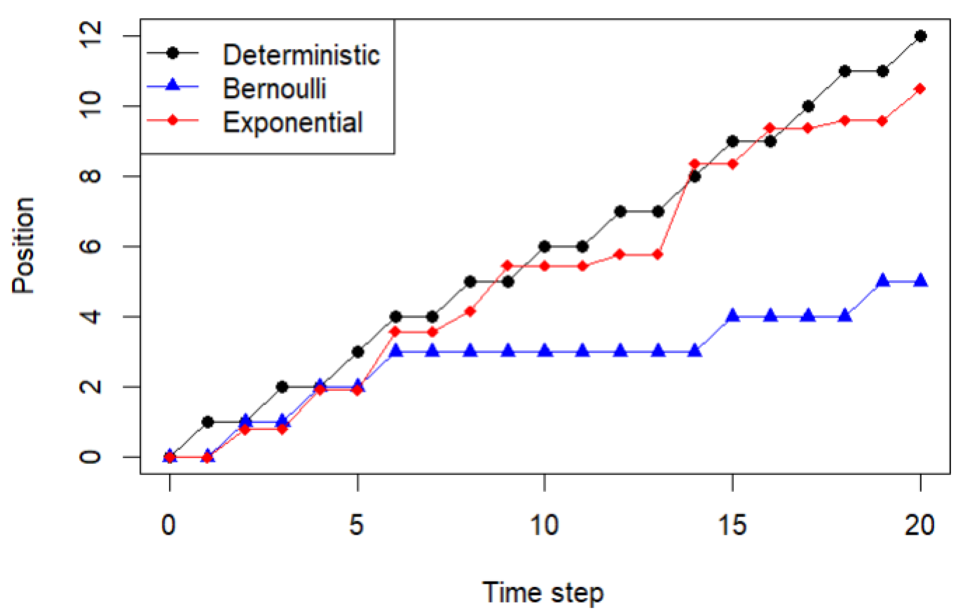
We present example trajectories of a particle for three different step-size mechanisms: deterministic, Bernoulli, and exponential. The simulations are performed for $n=20$ steps, with an initial move probability $r=0.5$ and two different persistence probabilities, $p=0.2$ and $p=0.8$. These examples illustrate how both the step-size distribution and the tendency to repeat the previous action influence the particle’s trajectory. In particular, lower persistence $(p=0.2)$ leads to frequent reversals in direction, while higher persistence $(p=0.5)$ produces smoother trajectories. The stochastic nature of Bernoulli and exponential step sizes introduces additional variability compared with the deterministic case, with exponential steps generating the largest fluctuations due to their unbounded, continuous nature.

Figure 2 shows that the deterministic path increases regularly due to the fixed step size, while the Bernoulli path exhibits additional variability arising from discrete random steps. The exponential path shows the largest fluctuations, reflecting the unbounded, continuous nature of the step sizes. In all cases, the persistence probability $p=0.8$ induces temporal correlation, causing trajectories to tend to continue their previous direction. Overall, this figure illustrates how step-size randomness and directional persistence jointly influence the particle’s motion.

Figure 3 shows that the deterministic path progresses in uniform steps but frequently reverses direction due to low persistence. The Bernoulli path exhibits additional variability from discrete random steps, occasionally stagnating when the step size is zero. The exponential path shows the largest fluctuations due to continuous, unbounded step sizes combined with frequent direction reversals. This figure illustrates how step-size distribution and directional persistence jointly influence particle trajectories.

3. Main Results

In this section we present our main results. We denote by $D_n$, the number of steps with size 0 from $\{1,\dots n\}$. Is the number of times that the elephants have decided not to move. The first result is about the first two moments of $D_n$ given in Equation (6).

Theorem 1.

For all $n\ge 1$, the mean and variance of $D_n$ are given by

$$\begin{array}{cc}\hfill \mathbb{E}\left[D_n\right]=& {\displaystyle \frac{1}{4(1-p)}}\left(2n(1-p)+(1-2r)\left[1-{(2p-1)}^n\right]\right),\hfill \end{array}$$

and

$$\begin{array}{cc}\hfill \mathbb{V}ar\left[D_n\right]=& {\displaystyle \frac{1-2r}{4(1-p)}}\left(1-{(2p-1)}^n\right)+{\displaystyle \frac{1}{4(1-p)}}(1-2r)\left(1-{(2p-1)}^{n-1}\right)n+{\displaystyle \frac{1}{2}}n\hfill \\ \hfill & +{\displaystyle \frac{(1-2r)}{4(1-p)}}\left[{\displaystyle \frac{(2p-1)}{2(1-p)}}\left(1-{(2p-1)}^{n-1}\right)-(n-1){(2p-1)}^n\right]\hfill \\ \hfill & -{\displaystyle \frac{(1-2r)}{8{(1-p)}^2{(2p-1)}^{n-1}}}\left(-1+{(2p-1)}^n+2n(1-p)\right)\hfill \\ \hfill & +{\displaystyle \frac{\left(2p-1\right)}{4\left(1-p\right)}}\left[(n-1)-{\displaystyle \frac{1}{2\left(1-p\right)}}\left(1-{(2p-1)}^{n-1}\right)\right]+{\displaystyle \frac{1}{4}}n(n-1)\hfill \\ \hfill & -{\displaystyle \frac{1}{16{(1-p)}^2}}{\left(2n(1-p)+(1-2r)\left[1-{(2p-1)}^n\right]\right)}^2.\hfill \end{array}$$

The exact distribution of $D_n$ is given in the following Theorem.

Theorem 2.

For all $1\le m\le n$, we have

$$\begin{array}{cc}\hfill \mathbb{P}\left(D_n=m\right)=& (1-r)\sum _{n_1+n_2=n-1,k_1+n_2=m-1,k_1\le n_1}{r}^{n_1-k_1}{(1-r)}^{k_1}{p}^{n_2}\left({\displaystyle \genfrac{}{}{0pt}{}{k_1}{n_1}}\right)\hfill \\ \hfill & +r{(1-r)}^m\sum _{n_1+n_2=n-1,n_1\ge m-1}{p}^{n_2}\left({\displaystyle \genfrac{}{}{0pt}{}{m}{n_1}}\right).\hfill \end{array}$$

Using the fact that, for all $k,l$ two integer numbers, we have

$$\mathbb{C}ov\left(D_{k+l},D_k\right)={\displaystyle \frac{1}{2}}\mathbb{P}\left({\widehat{Z}}_k=0\right){\left(2p-1\right)}^l\left[1-{\left(2p-1\right)}^k\left(1-2r\right)\right],$$

we deduce the following result, which clearly illustrates the symmetry phenomenon between the number of upward moves and the number of stops.

Theorem 3.

We have the following central limit theorem (CLT) with respect to $D_n$:

$$\sqrt{n}\left({\displaystyle \frac{D_n}{n}}-{\displaystyle \frac{1}{2}}\right)\stackrel{D}{⟶}\mathcal{N}\left(0,{\sigma }_D^2\right),$$

where ${\sigma }_D^2={lim}_{n\to \infty }{\displaystyle \frac{\mathbb{V}ar\left(D_n\right)}{n}}$.

Remark 1.

The number of stops $D_n$ was also studied in [6], but only in the context of the full-memory ERW, where it was shown that the expectation of $D_n$ is given by, for $n\ge 1$,

$$\mathbb{E}\left[D_n\right]={\displaystyle \frac{\Gamma (n+1-r)}{\Gamma (1-r)(9n-1)!}},$$

where, in this reference, r is the probability to stop at step n. Some other characteristics related to $D_n$ are given in the proofs.

The second part of our results concerns the process ${\widehat{Y}}_n$, representing the position of the elephant at time n.

Theorem 4.

For all fixed $n\ge 1$, the mean and variance of ${\widehat{Y}}_n$ are given by

$$\begin{array}{cc}\hfill \mathbb{E}\left[{\widehat{Y}}_n\right]& ={\displaystyle \frac{1}{4(1-p)}}\left(2n(1-p)-(1-2r)[1-{(2p-1)}^n]\right),\hfill \\ \\ \hfill \mathbb{V}ar\left[{\widehat{Y}}_n\right]& =\mathbb{V}ar\left[D_n\right]+{\sigma }^2\left(n-\mathbb{E}\left[D_n\right]\right).\hfill \end{array}$$

The distribution of ${\widehat{Y}}_n$ can be characterized by the moment-generating function, where the moment-generating function ${\Phi }_S\left(t\right)$ of a random variable S, when it exists, is defined as ${\Phi }_S\left(t\right)=\mathbb{E}\left[e^{tS}\right]$.

Theorem 5.

For all $n\ge 2$, the moment generating function of ${\widehat{Y}}_n$ is given by

$$\begin{array}{cc}\hfill {\Phi }_n\left(t\right)=& (1-r)\sum _{m=1}^n{\left({\Phi }_Z\left(t\right)\right)}^{n-m}\sum _{n_1+n_2=n-1,k_1+n_2=m-1,k_1\le n_1}{r}^{n_1-k_1}{(1-r)}^{k_1}{p}^{n_2}\left({\displaystyle \genfrac{}{}{0pt}{}{k_1}{n_1}}\right)\hfill \\ \hfill & + r\sum _{m=1}^n{\left({\Phi }_Z\left(t\right)\right)}^{n-m}{(1-r)}^m\sum _{n_1+n_2=n-1,n_1\ge m-1}{p}^{n_2}\left({\displaystyle \genfrac{}{}{0pt}{}{m}{n_1}}\right).\hfill \end{array}$$

The third result is about the central limit theorem with respect to ${\widehat{Y}}_n$.

Theorem 6.

When n goes to infinity, we have

$$\sqrt{n}\left({\displaystyle \frac{{\widehat{Y}}_n}{n}}-1+{\displaystyle \frac{D_n}{n}}\right)\stackrel{D}{⟶}\mathcal{N}\left(0,{\displaystyle \frac{{\sigma }^2}{2}}\right),$$

where ${\sigma }^2$ is the variance of $Z_1$.

4. Simulations

4.1. Curve of the Sequence ${\displaystyle \frac{\mathbb{E}\left(D_n\right)}{n}}$

Figure 4 displays the evolution of the ratio $R_n={\displaystyle \frac{\mathbb{E}\left(D_n\right)}{n}}$ as a function of time n for different parameter choices $(p,r)$. Regardless of the values of r and p, all trajectories rapidly converge to the same limiting value, approximately $R\approx 1/2$. This indicates that, asymptotically, the system spends about half of the time in state 0, independently of the initial conditions and transition probabilities. The convergence is very fast: after only a few hundred iterations, the curves become indistinguishable and remain stable around the limiting ratio.

4.2. Simulations of ${\displaystyle \frac{D_n}{n}}$

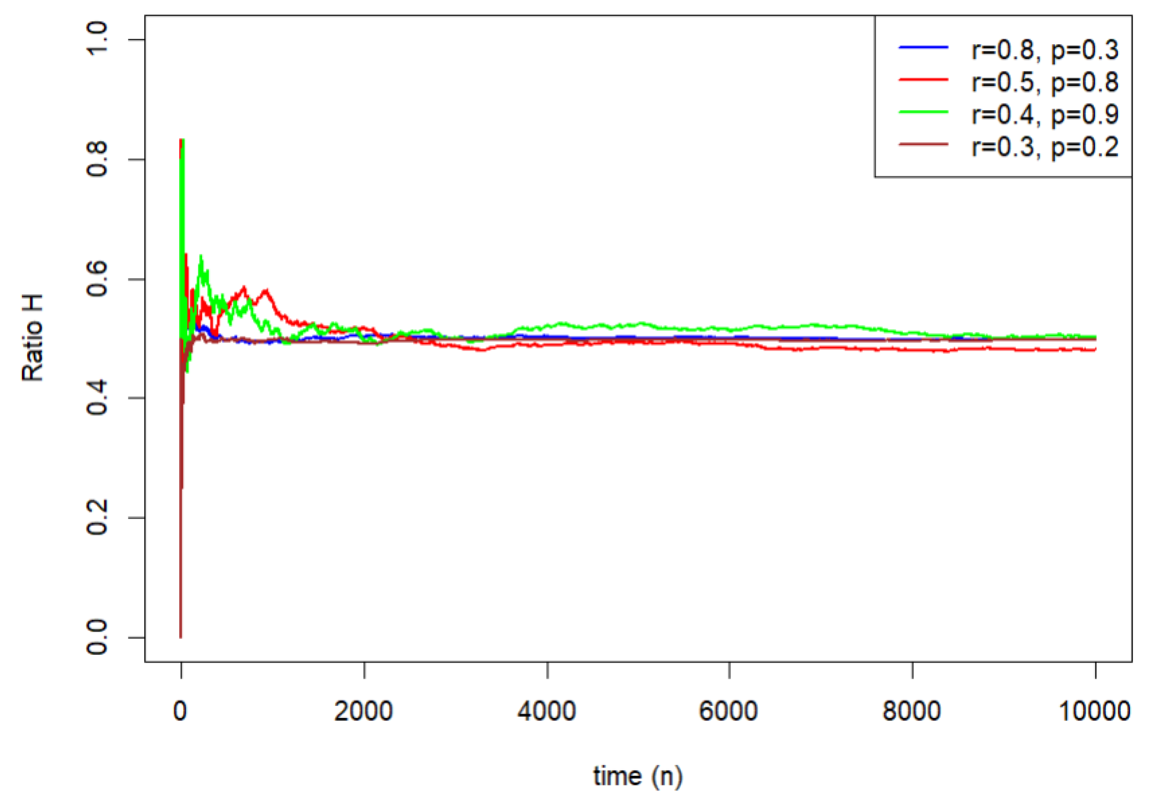
Figure 5 displays the evolution of the ratio $H_n={\displaystyle \frac{D_n}{n}}$ as a function of time n for different parameter values $(r,p)$. At the beginning, the trajectories show strong fluctuations, especially for $n<500$. As time increases, all curves gradually stabilize and converge toward similar limiting values around $H\approx 0.5$. This suggests that despite differences in the initial parameters $(r,p)$, the long-term behavior of the ratio H remains stable and relatively independent of the chosen values. The early-stage variability reflects sensitivity to initial conditions, whereas the convergence in the long run highlights the robustness of the system’s asymptotic properties.

4.3. Simulations of the CLT with Respect to $D_n$

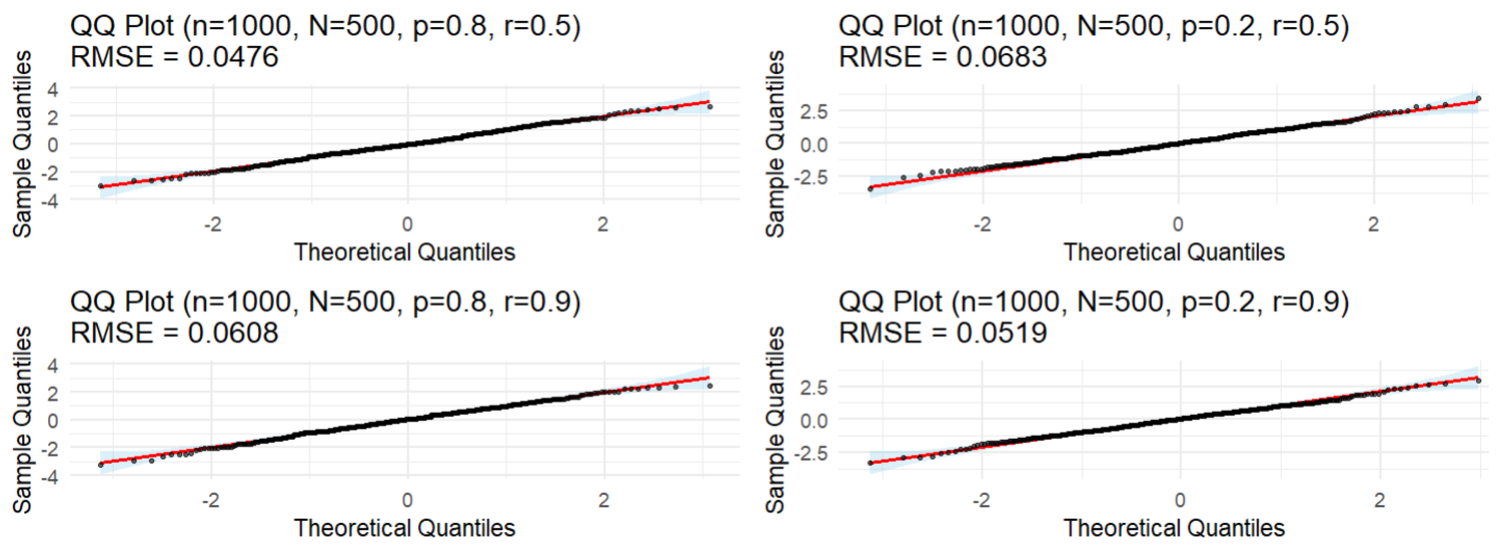
Across all panels in Figure 6, the empirical points lie close to the reference line, and the RMSE values remain small (below 0.07), supporting the adequacy of the normal approximation predicted by the central limit theorem. The persistence parameter p and the initial move probability r slightly affect tail alignment: higher persistence ($p=0.8$) with moderate r yields slightly larger deviations in the extremes, while lower persistence ($p=0.2$) produces comparatively smoother fits. Nevertheless, deviations remain minor and are reflected in the small RMSE values. Overall, the QQ plots confirm that for these parameter settings, the distribution of the standardized statistic is well approximated by a normal law, with only mild discrepancies in the tails.

By analyzing different combinations of parameters n, N, p, and r, in

Table 1. Normality tests for the statistic $D_n$.

n	N	p	r	Shapiro p	AD p	D’Agostino p	Jarque-Bera p	Skew	Kurtosis	RMSE (QQ)
1000	100	0.8	0.5	0.0734	0.0553	0.3744	0.3984	0.2062	−0.5213	0.1289
1000	100	0.9	0.4	0.7503	0.7294	0.9854	0.9656	0.0042	−0.1294	0.1459
1000	100	0.7	0.8	0.6884	0.4449	0.3716	0.4133	−0.2074	0.5020	0.0767
1000	100	0.6	0.2	0.1068	0.0777	0.1476	0.2449	−0.3408	−0.4590	0.0796
1000	500	0.8	0.5	0.3050	0.6493	0.8899	0.6237	−0.0149	−0.2108	0.0564
1000	500	0.9	0.4	0.3009	0.2340	0.4574	0.7217	−0.0804	−0.0740	0.0908
1000	500	0.7	0.8	0.0771	0.0300	0.9377	0.0962	−0.0084	−0.4738	0.0576
1000	500	0.6	0.2	0.2121	0.1353	0.1646	0.3287	−0.1509	−0.1255	0.0370
1000	1000	0.8	0.5	0.4920	0.9301	0.2997	0.5859	−0.0799	−0.0121	0.0385
1000	1000	0.9	0.4	0.6107	0.7053	0.2406	0.4919	0.0904	−0.0368	0.0522
1000	1000	0.7	0.8	0.4501	0.6176	0.3050	0.4085	−0.0790	−0.1342	0.0297
1000	1000	0.6	0.2	0.1838	0.1821	0.0691	0.1229	0.1405	0.1473	0.0281
5000	500	0.8	0.5	0.1475	0.1519	0.1459	0.3530	−0.1579	0.0135	0.0688
5000	500	0.9	0.4	0.8283	0.9572	0.6109	0.4931	0.0550	−0.2362	0.0577
5000	500	0.7	0.8	0.9353	0.8440	0.9381	0.9241	−0.0084	0.0854	0.0299
5000	500	0.6	0.2	0.8334	0.6808	0.5682	0.7689	−0.0617	−0.1001	0.0246
5000	1000	0.8	0.5	0.0572	0.0771	0.6327	0.8048	−0.0368	−0.0708	0.0530
5000	1000	0.9	0.4	0.5190	0.4786	0.2747	0.5219	−0.0841	−0.0538	0.0570
5000	1000	0.7	0.8	0.8795	0.7643	0.2864	0.5282	0.0821	0.0607	0.0238
5000	1000	0.6	0.2	0.7667	0.5681	0.2618	0.3759	0.0864	0.1307	0.0208
5000	5000	0.8	0.5	0.7309	0.8995	0.4333	0.4972	0.0271	−0.0614	0.0163
5000	5000	0.9	0.4	0.2042	0.1210	0.1990	0.2875	0.0444	0.0638	0.0323
5000	5000	0.7	0.8	0.3480	0.2778	0.2267	0.3971	−0.0418	0.0432	0.0150
5000	5000	0.6	0.2	0.3415	0.2645	0.4834	0.1517	0.0242	−0.1255	0.0125
10,000	1000	0.8	0.5	0.0844	0.4323	0.0308	0.0931	−0.1672	−0.0469	0.0500
10,000	1000	0.9	0.4	0.7007	0.8221	0.8965	0.7072	−0.0100	0.1274	0.0513
10,000	1000	0.7	0.8	0.4050	0.1315	0.1614	0.3744	−0.1080	0.0228	0.0309
10,000	1000	0.6	0.2	0.7549	0.7786	0.3642	0.6191	−0.0699	−0.0591	0.0210
10,000	5000	0.8	0.5	0.2430	0.4538	0.0737	0.0859	0.0619	0.0907	0.0221
10,000	5000	0.9	0.4	0.8403	0.6826	0.3134	0.5722	−0.0349	−0.0222	0.0229
10,000	5000	0.7	0.8	0.3847	0.2229	0.7748	0.2187	−0.0099	0.1192	0.0158
10,000	5000	0.6	0.2	0.3686	0.5618	0.5868	0.8148	−0.0188	0.0235	0.0120
10,000	10,000	0.8	0.5	-	0.2019	0.4898	0.7856	0.0169	−0.0039	0.0171
10,000	10,000	0.9	0.4	-	0.1200	0.7006	0.0878	−0.0094	−0.1064	0.0240
10,000	10,000	0.7	0.8	-	0.1464	0.2441	0.1870	−0.0285	0.0692	0.0126
10,000	10,000	0.6	0.2	-	0.1863	0.4941	0.7915	−0.0167	0.0013	0.0078

we can draw several conclusions.

1.

Effect of Sample Size per Sample (n)

(a)

As n increases, the data generally becomes more normal.

(b)

This is most clearly seen in the RMSE (QQ) column, which consistently decreases as n increases for fixed N, p, r.

(c)

Example: For $N=100$, $p=0.8$, $r=0.5$, RMSE drops from 0.1289 ($n=1000$) to 0.0564 ($n=5000$) to 0.0385 ($n=10,000$).

(d)

The p-values from the normality tests also tend to become larger (less significant) as n increases, further supporting this trend.

2.

Effect of Number of Samples/Replications (N)

(a)

As N increases, the data also becomes more normal.

(b)

This pattern is also very clear in the RMSE (QQ) column.

(c)

Example: For $n=5000$, $p=0.8$, $r=0.5$, RMSE drops from 0.0688 ($N=500$) to 0.0530 ($N=1000$) to 0.0163 ($N=5000$).

(d)

This suggests that the data generation process itself may produce a perfectly normal distribution only in the limit as the number of replications grows large.

3.

Effect of Parameters p and r

(a)

The effects of p and r are more subtle and interact with n and N.

(b)

There is no single, dominant pattern. For instance:

• Sometimes a combination like $p=0.7$, $r=0.8$ produces excellent normality (e.g., row 3, row 15).
• Other combinations like $p=0.6$, $r=0.2$ can show weaker normality for smaller n and N (e.g., row 4, row 8) but become perfectly normal with larger n and N (e.g., row 20, row 32).

(c)

This indicates that the impact of the data generation parameters (p, r) is complex and depends on the sample size.

4.

Agreement Between Tests

(a)

The four normality tests generally agree on the broad conclusion (normal vs. not normal) but often disagree on the specific p-value.

(b)

For very large n and N (e.g., $n=\mathrm{10,000}$, $N=\mathrm{10,000}$), the Shapiro-Wilk test returns NA. This is a known computational limitation; the test becomes too computationally expensive or unstable with very large sample sizes.

5.

Overall Normality

(a)

Despite some low p-values for smaller n and N, the Skewness and Kurtosis values are almost always very close to 0.

(b)

The RMSE values are consistently low, especially for larger n and N.

(c)

Conclusion: The data generation process produces distributions that are very close to normal, especially when the sample size (n) and the number of replications (N) are large. The deviations from normality detected by the tests in some scenarios are minor in a practical sense.

4.4. Simulations of the CLT with Respect to ${\widehat{Y}}_n$

Table 2. Normality tests for the statistic $\sqrt{n}\left({\displaystyle \frac{{\widehat{Y}}_n}{n}}-1+{\displaystyle \frac{D_n}{n}}\right)$.

n	N	p	r	Shapiro_p	AD_p	DAgostino_p	JarqueBera_p	Skew	Kurtosis	QQ_RMSE
1000	100	0.9	0.7	0.0463	0.1680	0.0177	0.0210	−0.579	3.715	0.1632
1000	100	0.5	0.4	0.3249	0.5554	0.4319	0.5485	0.182	2.605	0.1081
1000	100	0.3	0.2	0.5188	0.3811	0.5454	0.8483	−0.140	3.031	0.1068
1000	500	0.9	0.7	0.6002	0.5992	0.7017	0.6046	−0.041	2.796	0.0471
1000	500	0.5	0.4	0.4369	0.1138	0.9447	0.7695	−0.007	2.842	0.0571
1000	500	0.3	0.2	0.4542	0.5782	0.4844	0.4689	0.076	2.777	0.0525
1000	1000	0.9	0.7	0.7486	0.9600	0.7452	0.9323	0.025	3.029	0.0339
1000	1000	0.5	0.4	0.6739	0.6254	0.5693	0.8480	−0.044	2.984	0.0347
1000	1000	0.3	0.2	0.8592	0.9293	0.2925	0.5771	−0.081	3.010	0.0323
5000	500	0.9	0.7	0.4709	0.6903	0.2177	0.4189	−0.134	3.110	0.0535
5000	500	0.5	0.4	0.1679	0.3629	0.1323	0.2175	0.164	2.801	0.0646
5000	500	0.3	0.2	0.0405	0.1880	0.0405	0.1114	−0.224	2.898	0.0763
5000	1000	0.9	0.7	0.5634	0.2362	0.3444	0.5558	−0.073	2.916	0.0360
5000	1000	0.5	0.4	0.7521	0.5165	0.5408	0.8205	0.047	2.975	0.0325
5000	1000	0.3	0.2	0.9102	0.8762	0.9787	0.8108	0.002	2.900	0.0291
5000	5000	0.9	0.7	0.4359	0.1218	0.7831	0.6190	0.010	2.935	0.0191
5000	5000	0.5	0.4	0.2589	0.2820	0.4984	0.1607	0.023	3.124	0.0225
5000	5000	0.3	0.2	0.4999	0.4140	0.5879	0.5095	−0.019	3.071	0.0183
10,000	1000	0.9	0.7	0.1261	0.0238	0.5905	0.7085	−0.041	2.902	0.0489
10,000	1000	0.5	0.4	0.5546	0.2731	0.7248	0.5426	0.027	3.163	0.0387
10,000	1000	0.3	0.2	0.1446	0.0520	0.6166	0.3184	0.039	2.779	0.0461
10,000	3000	0.9	0.7	0.6385	0.1898	0.3814	0.4425	−0.039	2.917	0.0213
10,000	3000	0.5	0.4	0.6471	0.7873	0.7175	0.4873	0.016	3.102	0.0247
10,000	3000	0.3	0.2	0.0193	0.1318	0.3624	0.0395	0.041	3.212	0.0355
10,000	5000	0.9	0.7	0.8361	0.8834	0.8570	0.9717	0.006	2.989	0.0147
10,000	5000	0.5	0.4	0.0709	0.3440	0.0295	0.0640	−0.075	3.060	0.0255
10,000	5000	0.3	0.2	0.1867	0.4124	0.3670	0.4591	−0.031	3.060	0.0217

reports normality assessment results for different sample sizes $n\in \{1000, 5000, \mathrm{10,000}\}$, numbers of Monte Carlo replications N, and parameter pairs $(p,r)\in \left\{\right(0.9, 0.7), (0.5, 0.4), (0.3, 0.2\left)\right\}$. Several normality tests (Shapiro–Wilk, Anderson–Darling, D’Agostino, Jarque–Bera) are presented alongside skewness, kurtosis, and QQ-plot RMSE. As n increases, all tests generally indicate improved agreement with the normal distribution, with p-values moving away from the 5% significance threshold. Skewness remains near zero and kurtosis close to 3 for $n\ge 5000$, while QQ-plot RMSE decreases, confirming visual closeness to normality. Deviations are most pronounced at $n=1000$ for $(p,r)=(0.9,0.7)$, where tests occasionally reject normality due to negative skew and excess kurtosis. Overall, these results provide strong evidence of a Central Limit Theorem effect: the standardized statistic converges rapidly to Gaussian behavior as n grows, with excellent agreement across all tests for $n\ge 5000$.

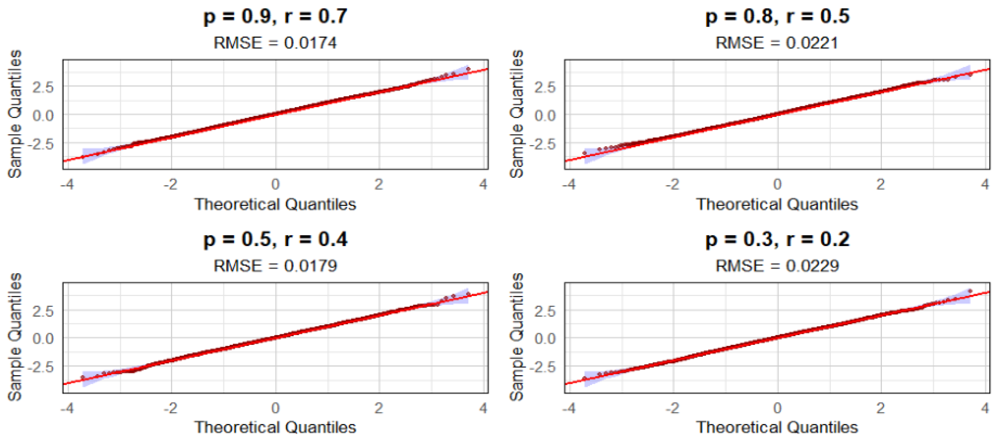
The QQ plots in Figure 7 demonstrate robust asymptotic normality of the standardized statistic $\sqrt{n}\left({\displaystyle \frac{{\widehat{Y}}_n}{n}}-1+{\displaystyle \frac{D_n}{n}}\right)$ across all parameter configurations, with exceptional alignment to the theoretical normal distribution evidenced by near-perfect linearity along the reference line and complete containment within the 95% confidence bands. The remarkably low RMSE values ($0.0174$–$0.0229$) indicate minimal quantile deviation, with the highest persistence parameters $(p=0.9,r=0.7)$ yielding the most precise approximation and even the lowest persistence case $(p=0.3,r=0.2)$ maintaining excellent fit. The absence of systematic deviations confirms no detectable skewness or heavy-tailed behavior, validating the Central Limit Theorem’s applicability and ensuring reliable statistical inference using normal approximations across the entire parameter space.

5. Some Characteristics of the Distribution of the Process ${\widehat{\mathit{Z}}}_{\mathit{n}}$

We start with the probability that at step n the process does not move. Let $u_n:=\mathbb{P}\left({\widehat{Z}}_n=0\right)$. Due to Equation (4), the following lemma is straightforward.

Lemma 1.

The sequence $u_n$ satisfies, $u_1=1-r$ and, for $n\ge 2$,

$$u_n=\left(2p-1\right)u_{n-1}+\left(1-p\right),$$

the solution is given by

$$u_n={\left(2p-1\right)}^{n-1}\left({\displaystyle \frac{1}{2}}-r\right)+{\displaystyle \frac{1}{2}}.$$

(7)

In the rest of this section, we focus on explicitly calculating the first two moments of the processes ${\widehat{Z}}_n$ and ${\widehat{Y}}_n$. These moments will be useful later for studying the distributions of these two processes, as well as for deriving the asymptotic behavior in probability of the process ${\widehat{Y}}_n$. Denote $m_{n,1}:=\mathbb{E}\left[{\widehat{Z}}_n\right]$, from the last lemma we deduce

Corollary 1.

The mean $m_{n,1}$ is given by, for all $n\ge 1$

$$m_{n,1}={\displaystyle \frac{1}{2}}-\left({\displaystyle \frac{1}{2}}-r\right){(2p-1)}^{n-1}.$$

Proof. 

It is clear, from the model, that $m_{1,1}=\mathbb{E}\left[{\widehat{Z}}_1\right]=\mathbb{E}\left[{\widehat{Y}}_1\right]=r$. For $n\ge 2$, one has

$$\begin{array}{cc}\hfill m_{n,1}=& \mathbb{E}\left[Z_n\left({\mathbf{1}}_{A_n}{\mathbf{1}}_{\{{\widehat{Z}}_{n-1}\ne 0\}}+{\mathbf{1}}_{{\overline{A}}_n}{\mathbf{1}}_{\{{\widehat{Z}}_{n-1}=0\}}\right)\right]\hfill \\ \hfill =& \mathbb{E}\left[Z_n\right]\left[\mathbb{E}\left[{\mathbf{1}}_{A_n}\right]\mathbb{E}\left[{\mathbf{1}}_{\{{\widehat{Z}}_{n-1}\ne 0\}}\right]+\mathbb{E}\left[{\mathbf{1}}_{{\overline{A}}_n}\right]\mathbb{E}\left[{\mathbf{1}}_{\{{\widehat{Z}}_{n-1}=0\}}\right]\right].\hfill \end{array}$$

Use the identities

$$\mathbb{E}\left[Z_n\right]=1,\mathbb{E}\left[{\mathbf{1}}_{A_n}\right]=p,\mathbb{E}\left[{\mathbf{1}}_{\{{\widehat{Z}}_{n-1}=0\}}\right]=u_{n-1},$$

(8)

to conclude that

$$\begin{array}{cc}\hfill m_{n,1}=& p\left(1-u_{n-1}\right)+\left(1-p\right)u_{n-1}=p-(2p-1)u_{n-1}.\hfill \end{array}$$

Using, now, the explicit expression of $u_n$ in Lemma 1, to get

$$m_{n,1}={\displaystyle \frac{1}{2}}-\left({\displaystyle \frac{1}{2}}-r\right){(2p-1)}^{n-1}.$$

 □

Lemma 2.

Let $m_{n,2}:=\mathbb{E}\left[{\widehat{Z}}_n^2\right]$, the second moment of ${\widehat{Z}}_n$. The sequence $m_{n,2}$ satisfies the following recursive equation:

$$m_{n,2}=(1+{\sigma }^2)\left(p-(2p-1)u_{n-1}\right),$$

(9)

and its explicit expression is given by the following, for all $n\ge 1$:

$$m_{n,2}={\displaystyle \frac{1}{2}}(1+{\sigma }^2)-(1+{\sigma }^2)\left({\displaystyle \frac{1}{2}}-r\right){(2p-1)}^{n-1}.$$

(10)

Proof. 

One has

$$\begin{array}{cc}\hfill m_{n,2}=& \mathbb{E}\left[Z_n^2\right]\left[\mathbb{E}\left[{\mathbf{1}}_{A_n}\right]\mathbb{E}\left[{\mathbf{1}}_{\{{\widehat{Z}}_{n-1}\ne 0\}}\right]+\mathbb{E}\left[{\mathbf{1}}_{{\overline{A}}_n}\right]\mathbb{E}\left[{\mathbf{1}}_{\{{\widehat{Z}}_{n-1}=0\}}\right]\right].\hfill \end{array}$$

Using Equation (8) and $\mathbb{V}ar\left[Z_n\right]={\sigma }^2$, then $m_{n,2}$ satisfies

$$\begin{array}{cc}\hfill m_{n,2}=& (1+{\sigma }^2)\left(p-(2p-1)u_{n-1}\right)\hfill \\ \hfill =& (1+{\sigma }^2)(p-{\left(2p-1\right)}^{n-1}\left({\displaystyle \frac{1}{2}}-r\right)-p+{\displaystyle \frac{1}{2}})\hfill \\ \hfill =& (1+{\sigma }^2)\left({\displaystyle \frac{1}{2}}-{\left(2p-1\right)}^{n-1}\left({\displaystyle \frac{1}{2}}-r\right)\right)\hfill \end{array}$$

and its explicit formula is given by

$$m_{n,2}={\displaystyle \frac{1}{2}}(1+{\sigma }^2)-(1+{\sigma }^2)\left({\displaystyle \frac{1}{2}}-r\right){(2p-1)}^{n-1}.$$

 □

6. Number of Stops of the Process

By stop, we mean the fact that the walk does not move. For all $n\ge 1$, let $D_n$ be the number of times that the walk does not move, then $n-D_n$ is the number of moves up to time n. Recall that $D_n$ is defined by

$$D_n=\#\left\{1\le k\le n,{\widehat{Z}}_k=0\right\}.$$

The process $D_n$ plays a crucial role in the study of the process ${\widehat{Y}}_n$ due to a distributional identity linking the two processes. For this reason, we dedicate this section to the analysis of $D_n$, which will later be used to deduce the behavior of the process ${\widehat{Y}}_n$.

6.1. Proof of Theorem 1

Since the sequence ${\left(D_n\right)}_n$ satisfies, for all $n\ge 1$,

$$D_n=D_{n-1}+{\mathbf{1}}_{\{{\widehat{Z}}_n=0\}}$$

we deduce that, the mean $d_n:=E\left[D_n\right]$ satisfies

$$\begin{array}{cc}\hfill d_n& =d_{n-1}+u_n=\sum _{k=1}^n{u}_k.\hfill \end{array}$$

The proof can be achieved using Equation (7).

Remark 2.

The symmetry phenomenon between the number of times the elephant decides to move upward and the number of times it decides to remain stationary is revealed on average. In fact, as a direct consequence of the last Lemma, we deduce that, for $p\ne 1$,

$$\underset{n}{lim}{\displaystyle \frac{\mathbb{E}\left[D_n\right]}{n}}={\displaystyle \frac{1}{2}}.$$

(11)

Recall that the variable $D_n$ can be given by $D_n={\sum }_{k=1}^n{\mathbb{I}}_{\{{\widehat{Z}}_k=0\}}.$ We start by computing the second moment of $D_n$. we have

$$\begin{array}{cc}\hfill \mathbb{E}\left[D_n^2\right]& =\sum _{k=1}^n\mathbb{P}\left({\widehat{Z}}_k=0\right)+2\sum _{1\le l<k\le n}\mathbb{P}\left({\widehat{Z}}_k=0,{\widehat{Z}}_l=0\right)\hfill \\ \hfill & =\sum _{k=1}^n\mathbb{P}\left({\widehat{Z}}_k=0\right)+2\sum _{1\le l<k\le n}\mathbb{P}\left({\widehat{Z}}_k=0|{\widehat{Z}}_l=0\right)\mathbb{P}\left({\widehat{Z}}_l=0\right).\hfill \end{array}$$

Remark that $\mathbb{P}\left({\widehat{Z}}_k=0|{\widehat{Z}}_l=0\right)$ is the probability that the step of the same walk at time $k-l$ equals 0 for $r=1-p$. Then,

$$\mathbb{P}\left({\widehat{Z}}_k=0|{\widehat{Z}}_l=0\right)={\left(2p-1\right)}^{k-l-1}\left(p-{\displaystyle \frac{1}{2}}\right)+{\displaystyle \frac{1}{2}}.$$

We deduce,

$$\begin{array}{cc}\hfill \mathbb{E}\left[D_n^2\right]=& \sum _{k=1}^n\left[{\left(2p-1\right)}^{k-1}\left({\displaystyle \frac{1}{2}}-r\right)+{\displaystyle \frac{1}{2}}\right]\hfill \\ \hfill & +2\sum _{1\le l<k\le n}\left[{\left(2p-1\right)}^{k-l-1}\left(p-{\displaystyle \frac{1}{2}}\right)+{\displaystyle \frac{1}{2}}\right]\left[{\left(2p-1\right)}^{l-1}\left({\displaystyle \frac{1}{2}}-r\right)+{\displaystyle \frac{1}{2}}\right]\hfill \\ \hfill =& \sum _{k=1}^n\left[{\left(2p-1\right)}^{k-1}\left({\displaystyle \frac{1}{2}}-r\right)+{\displaystyle \frac{1}{2}}\right]\hfill \\ \hfill & +2\sum _{l=1}^{n-1}\left[{\left(2p-1\right)}^{l-1}\left({\displaystyle \frac{1}{2}}-r\right)+{\displaystyle \frac{1}{2}}\right]\sum _{k=l+1}^n\left[{\left(2p-1\right)}^{k-l-1}\left(p-{\displaystyle \frac{1}{2}}\right)+{\displaystyle \frac{1}{2}}\right]\hfill \\ \hfill =& \sum _{k=1}^n\left[{\left(2p-1\right)}^{k-1}\left({\displaystyle \frac{1}{2}}-r\right)+{\displaystyle \frac{1}{2}}\right]\hfill \\ \hfill & +2\sum _{l=1}^{n-1}\left[{\left(2p-1\right)}^{l-1}\left({\displaystyle \frac{1}{2}}-r\right)+{\displaystyle \frac{1}{2}}\right]\sum _{j=0}^{n-(l+1)}\left[{\left(2p-1\right)}^j\left(p-{\displaystyle \frac{1}{2}}\right)+{\displaystyle \frac{1}{2}}\right].\hfill \end{array}$$

Using some identities about geometric sums, we obtain the following:

$$\begin{array}{cc}\hfill \mathbb{E}\left[D_n^2\right]=& \sum _{k=1}^n\left[{\left(2p-1\right)}^{k-1}\left({\displaystyle \frac{1}{2}}-r\right)+{\displaystyle \frac{1}{2}}\right]\hfill \\ \hfill & +2\sum _{l=1}^{n-1}\left[{\left(2p-1\right)}^{l-1}\left({\displaystyle \frac{1}{2}}-r\right)+{\displaystyle \frac{1}{2}}\right]\left[\left(2p-1\right){\displaystyle \frac{1-{\left(2p-1\right)}^{n-l}}{4\left(1-p\right)}}+{\displaystyle \frac{n-l}{2}}\right]\hfill \\ \hfill =& {\displaystyle \frac{1}{2}}\sum _{k=1}^n\left[{\left(2p-1\right)}^{k-1}\left(1-2r\right)+1\right]+{\displaystyle \frac{\left(1-2r\right)}{4\left(1-p\right)}}\sum _{l=1}^{n-1}\left[{\left(2p-1\right)}^l\right]\left[1-{\left(2p-1\right)}^{n-l}\right]\hfill \\ \hfill & +\left(1-2r\right)\sum _{l=1}^{n-1}\left[{\left(2p-1\right)}^{l-1}\right]\left[{\displaystyle \frac{n-l}{2}}\right]+{\displaystyle \frac{\left(2p-1\right)}{4\left(1-p\right)}}\sum _{l=1}^{n-1}\left[1-{\left(2p-1\right)}^{n-l}\right]+\sum _{l=1}^{n-1}{\displaystyle \frac{n-l}{2}}.\hfill \end{array}$$

Then we have

$$\begin{array}{cc}\hfill \mathbb{E}\left[D_n^2\right]=& {\displaystyle \frac{1-2r}{4(1-p)}}\left(1-{(2p-1)}^n\right)+{\displaystyle \frac{1}{2}}n\hfill \\ \hfill & +{\displaystyle \frac{1}{8{(1-p)}^2}}(1-2r)(2p-1)\left(1-{(2p-1)}^{n-1}\right)-{\displaystyle \frac{1-2r}{4(1-p)}}(n-1){(2p-1)}^n\hfill \\ \hfill & +{\displaystyle \frac{1}{4(1-p)}}(1-2r)\left(1-{(2p-1)}^{n-1}\right)n\hfill \\ \hfill & -{\displaystyle \frac{(1-2r)}{8{(1-p)}^2{(2p-1)}^{n-1}}}\left(-1+{(2p-1)}^n+2n(1-p)\right)\hfill \\ \hfill & +{\displaystyle \frac{\left(2p-1\right)}{4\left(1-p\right)}}(n-1)-{\displaystyle \frac{\left(2p-1\right)}{8{\left(1-p\right)}^2}}\left(1-{(2p-1)}^{n-1}\right)+{\displaystyle \frac{1}{4}}n(n-1)\hfill \end{array}$$

Remark 3.

When p is close to 1, we have the following asymptotic for the second moment of $D_n$:

$$\mathbb{E}\left[D_n^2\right]\approx {\displaystyle \frac{n^2}{4}}+({\displaystyle \frac{3}{4}}-r)n.$$

The following convergence in probability holds.

Corollary 2.

When n goes to infinity, we have

$${\displaystyle \frac{D_n}{n}}\stackrel{\mathbb{P}}{⟶}{\displaystyle \frac{1}{2}}.$$

Proof. 

Since ${lim}_{n\to \infty }\mathbb{V}ar\left[D_n\right]/n^2=0$, and using Theorem 2.2.4 [8] (p. 56), we deduce

$${\displaystyle \frac{D_n-\mathbb{E}\left[D_n\right]}{n}}\stackrel{\mathbb{P}}{⟶}0\mathrm{as} n\to \infty .$$

The desired result is obtained using (11). □

Corollary 3.

When n goes to infinity, we have

$$n-D_n\stackrel{a.s}{⟶}+\infty .$$

Proof. 

From the last result, we deduce that

$$D_n\stackrel{\mathbb{P}}{⟶}+\infty .$$

Since $n\to D_n$ is an increasing sequence, we conclude that

$$D_n\stackrel{a.s}{⟶}+\infty .$$

On the other hand, by expressing $n-D_n$ as

$$n-D_n=\sum _{k=1}^n{\mathbf{1}}_{\{{\widehat{Z}}_k\ne 0\}}=\sum _{k=1}^n{\mathbf{1}}_{\{{\widehat{Y}}_{k-1}\ne {\widehat{Y}}_k\}},$$

we deduce, using the same arguments as for $D_n$, that $n-D_n\stackrel{a.s}{⟶}+\infty .$ □

6.2. Proof of Theorem 2

Recall that, $\mathbb{P}\left({\widehat{Z}}_1\ne 0\right)=r,\mathbb{P}\left({\widehat{Z}}_1=0\right)=1-r.$ In order to study the distribution of $D_n$, we employee the bi-variate generating function $\Psi (x,y)$ defined on ${(0,1)}^2$ and given by

$$\Psi (x,y)=\sum _{1\le m\le n}\mathbb{P}\left(D_n=m\right)x^{n-m}{y}^m.$$

The generating series method is a highly effective tool for studying this type of model. It generally allows researchers to derive the exact distribution of the random walk or, at the very least, its asymptotic behavior. For an example of the application of this method, we refer the book [9]. The following Theorem will help us to obtain the exact distribution of $D_n$.

Theorem 7.

The expression of $\Psi (x,y)$ is given by

$$\begin{array}{cc}\hfill \Psi (x,y)=& (1-r)\sum _{0\le k_1\le n_1,n_2\ge 0}{r}^{n_1-k_1}{(1-r)}^{k_1}{p}^{n_2}\left({\displaystyle \genfrac{}{}{0pt}{}{k_1}{n_1}}\right)y^{k_1+n_2+1}{x}^{n_1-k_1}\hfill \\ \hfill & +r(1-r)\sum _{0\le k_1\le n_1,n_2\ge 0}{(1-r)}^{k_1}{p}^{n_2}\left({\displaystyle \genfrac{}{}{0pt}{}{k_1}{n_1}}\right)y^{k_1+1}{x}^{n_1+n_2-k_1}.\hfill \end{array}$$

To prove Theorem 7, we need the following lemma

Lemma 3.

For $m\ge 1$ and $n\ge m+1$, we have

$$\mathbb{P}\left(D_n=m\right)=r\mathbb{P}\left(D_{n-1}=m\right)+\left(1-r\right)\mathbb{P}\left(D_{n-1}=m-1\right)$$

Proof. 

For $m\ge 1,n\ge m+1$, we have

$$\begin{array}{cc}\hfill \mathbb{P}\left(D_n=m\right)& =\mathbb{P}\left(D_n=m,{\widehat{Z}}_1\ne 0\right)+\mathbb{P}\left(D_n=m,{\widehat{Z}}_1=0\right)\hfill \\ \hfill & =\mathbb{P}\left(D_n=m|{\widehat{Z}}_1\ne 0\right)\mathbb{P}\left({\widehat{Z}}_1\ne 0\right)+\mathbb{P}\left(D_n=m|{\widehat{Z}}_1=0\right)\mathbb{P}\left({\widehat{Z}}_1=0\right)\hfill \\ \hfill & =\mathbb{P}\left(D_{n-1}=m\right)\mathbb{P}\left({\widehat{Z}}_1\ne 0\right)+\mathbb{P}\left(D_{n-1}=m-1\right)\mathbb{P}\left({\widehat{Z}}_1=0\right)\hfill \\ \hfill & =r\mathbb{P}\left(D_{n-1}=m\right)+\left(1-r\right)\mathbb{P}\left(D_{n-1}=m-1\right).\hfill \end{array}$$

 □

On the other hand, we can verify that

Lemma 4.

For all $n\ge 1$,

$$\begin{array}{cc}\hfill \mathbb{P}\left(D_n=1\right)& =(1-p)p^{n-2}+(n-2)r{(1-p)}^2{p}^{n-3},\hfill \\ \hfill \mathbb{P}\left(D_n=n\right)& =(1-p)p^{n-1},\hfill \\ \hfill \mathbb{P}\left(D_n=0\right)& =r{p}^{n-1},\hfill \\ \hfill \mathbb{P}\left(D_1=1\right)& =(1-r).\hfill \end{array}$$

Proof of Thorem 7.

Using Lemmas 3 and 4, we have

$$\begin{array}{cc}\hfill \Psi (x,y)=& \sum _{1\le m\le n}\mathbb{P}\left(D_n=m\right)x^{n-m}{y}^m\hfill \\ \hfill =& \mathbb{P}\left(D_1=1\right)y+\sum _{n=2}^{+\infty }\sum _{m=1}^n\mathbb{P}(D_n=m)x^{n-m}{y}^m\hfill \\ \hfill =& \mathbb{P}\left(D_1=1\right)y+\sum _{n=2}^{+\infty }\mathbb{P}(D_n=n)y^n+\sum _{n=2}^{+\infty }\sum _{m=1}^{n-1}\mathbb{P}(D_n=m)x^{n-m}{y}^m\hfill \\ \hfill =& (1-r)y+(1-r)\sum _{n=2}^{+\infty }{p}^{n-1}{y}^n+\sum _{n=2}^{+\infty }\sum _{m=1}^{n-1}\mathbb{P}(D_n=m)x^{n-m}{y}^m\hfill \\ \hfill =& (1-r)y+(1-r)p{y}^2\sum _{n=2}^{+\infty }{\left(py\right)}^n+r\sum _{n=2}^{+\infty }\sum _{m=1}^{n-1}\mathbb{P}(D_{n-1}=m)x^{n-m}{y}^m\hfill \\ \hfill & +(1-r)\sum _{n=2}^{+\infty }\sum _{m=1}^{n-1}\mathbb{P}(D_{n-1}=m-1)x^{n-m}{y}^m\hfill \end{array}$$

$$\begin{array}{cc}\hfill \Psi (x,y)=& (1-r)y+(1-r)p{\displaystyle \frac{y^2}{1-py}}+r\sum _{n=1}^{+\infty }\sum _{m=1}^n\mathbb{P}(D_n=m)x^{n-m+1}{y}^m\hfill \\ \hfill & +(1-r)\sum _{n=1}^{+\infty }\sum _{m=0}^n\mathbb{P}(D_n=m)x^{n-m}{y}^{m+1}\hfill \\ \hfill =& (1-r)y+(1-r)p{\displaystyle \frac{y^2}{1-py}}+rx\sum _{1\le m\le n}\mathbb{P}(D_n=m)x^{n-m}{y}^m\hfill \\ \hfill & +(1-r)y\sum _{1\le m\le n}\mathbb{P}(D_n=m)x^{n-m}{y}^m+(1-r)y\sum _{n=1}^{+\infty }\mathbb{P}(D_n=0)x^n\hfill \\ \hfill =& (1-r)y+(1-r)p{\displaystyle \frac{y^2}{1-py}}+rx\Psi (x,y)+(1-r)y\Psi (x,y)+(1-r)ry\sum _{n=1}^{+\infty }{p}^{n-1}{x}^n\hfill \\ \hfill =& (1-r)y+(1-r)p{\displaystyle \frac{y^2}{1-py}}+rx\Psi (x,y)+(1-r)y\Psi (x,y)+r(1-r)y{\displaystyle \frac{x}{1-px}}.\hfill \end{array}$$

As a conclusion, we have

$$\begin{array}{cc}\hfill \Psi (x,y)=& {\displaystyle \frac{1}{1-rx-(1-r)y}}\left[(1-r)y+p(1-r){\displaystyle \frac{y^2}{1-py}}+r(1-r)y{\displaystyle \frac{x}{1-px}}\right]\hfill \\ \\ \hfill =& {\displaystyle \frac{1}{1-rx-(1-r)y}}\left[(1-r){\displaystyle \frac{y}{1-py}}+r(1-r)y{\displaystyle \frac{x}{1-px}}\right]\hfill \\ \\ \hfill =& {\displaystyle \frac{(1-r)y}{1-rx-(1-r)y}}\left[{\displaystyle \frac{1}{1-py}}+r{\displaystyle \frac{x}{1-px}}\right].\hfill \end{array}$$

The terms on the right-hand side, in the last equality, can be given by

$$\begin{array}{cc}\hfill {\displaystyle \frac{(1-r)y}{1-rx-(1-r)y}}=& (1-r)\sum _{n_1=0}^{+\infty }\sum _{k_1=0}^{n_1}{r}^{n_1-k_1}{(1-r)}^{k_1}\left({\displaystyle \genfrac{}{}{0pt}{}{k_1}{n_1}}\right)y^{k_1+1}{x}^{n_1-k_1}\hfill \\ \hfill {\displaystyle \frac{1}{1-py}}=& \sum _{n_2=0}^{+\infty }{p}^{n_2}{y}^{n_2}\hfill \\ \hfill r{\displaystyle \frac{x}{1-px}}=& r\sum _{n_3=0}^{+\infty }{p}^{n_3}{x}^{n_3+1}.\hfill \end{array}$$

 □

Proof of Theorem 2.

Using the expression of $\Psi (x,y)$ in Theorem 7, and using the Taylor expansion, with respect to x and y, we deduce that, for all integers k and l we have

$$\left[x^k{y}^l\right]=\mathbb{P}\left(D_{k+l}=l\right).$$

 □

7. Distribution of ${\widehat{\mathit{Y}}}_{\mathit{n}}$

For t real number, denote by ${\Phi }_n\left(t\right)=\mathbb{E}\left[e^{t{\widehat{Y}}_n}\right]$ the moment generating function of ${\widehat{Y}}_n$. On the other hand, it is clear that

$${\widehat{Y}}_n\stackrel{D}{=}\sum _{k=0}^{n-D_n}{Z}_k.$$

(12)

Using Corollary 3, we can conclude using the law of large numbers that

Corollary 4.

We have

$${\displaystyle \frac{{\widehat{Y}}_n}{n}}\stackrel{\mathbb{P}}{⟶}{\displaystyle \frac{1}{2}}.$$

7.1. Proof of Theorem 4

The proof is based on the identity given in Equation (12) and Theorem 1.

7.2. Proof of Theorem 5

For all $n\ge 1$ and for all complex number z, let

$${\Psi }_n\left(z\right)=\sum _{m=1}^n\mathbb{P}(D_n=m)z^{n-m}.$$

Then

$${\Phi }_n\left(t\right)=\mathbb{E}\left[e^{t{\widehat{Y}}_n}\right]=\mathbb{E}\left[{\Phi }_Z{\left(t\right)}^{n-D_n}\right]=\sum _{m=0}^n\mathbb{P}(D_n=m){\Phi }_Z{\left(t\right)}^{n-m}={\Psi }_n\left({\Phi }_Z\left(t\right)\right).$$

Finally, we finish the proof using the exact expression of ${\Psi }_n\left(t\right)$.

Remark 4.

Using the exact expression of ${\Phi }_n\left(t\right)$, one can derive, in an alternative form—as a sum—the expectation and variance of ${\widehat{Y}}_n$. Consequently, new identities that may be useful in combinatorics are obtained:

$$\mathbb{E}\left[{\widehat{Y}}_n\right]={\displaystyle \frac{d}{dt}}{\Phi }_n\left(t\right){|}_{t=0}\mathit{and}\mathbb{E}\left[{\widehat{Y}}_n^2\right]={\displaystyle \frac{d^2}{d{t}^2}}{\Phi }_n\left(t\right){|}_{t=0}.$$

7.3. Proof of Theorem 6

By Equation (12), and using Corollary 3, using the central limit theorem, we obtain

$${\displaystyle \frac{1}{\sqrt{n-D_n}}}\left({\widehat{Y}}_n-\left(n-D_n\right)\right)\stackrel{D}{⟶}\mathcal{N}\left(0,{\sigma }^2\right).$$

On the other hand, when n goes to infinity, and by Corollary (2), we have

$$\sqrt{{\displaystyle \frac{n}{n-D_n}}}={\displaystyle \frac{1}{\sqrt{1-\frac{D_n}{n}}}}\stackrel{\mathbb{P}}{⟶}\sqrt{2}.$$

Then

$$\begin{array}{cc}\hfill {\displaystyle \frac{1}{\sqrt{n-D_n}}}\left({\widehat{Y}}_n-\left(n-D_n\right)\right))& ={\displaystyle \frac{1}{\sqrt{n}\sqrt{1-\frac{D_n}{n}}}}\left({\widehat{Y}}_n-\left(n-D_n\right)\right))\hfill \\ \hfill & ={\displaystyle \frac{\sqrt{n}}{\sqrt{1-\frac{D_n}{n}}}}\left({\displaystyle \frac{{\widehat{Y}}_n}{n}}-1+{\displaystyle \frac{D_n}{n}}\right).\hfill \end{array}$$

8. Conclusions and Perspectives

In this work, we successfully derived the explicit distribution of the random walk ${\widehat{Y}}_n$ as well as the number of stops $D_n$. This model represents a modification of the framework studied in [10] and also draws inspiration from the model presented in [5,6]. The main result of this paper, which is the position of the elephant in each time step n, is the exact distribution of this process at each step n. This result was achieved through the study of the number of stops or delays $D_n$, using the bivariate generating series tool.

Beyond exact distributions and asymptotic laws, our analysis highlights the fundamental role of binary symmetry between repetition and inversion of past actions. This structural symmetry provides a unifying perspective for interpreting the probabilistic dynamics of the model and suggests potential applications in physics, combinatorics, and memory-based random processes where such balanced opposing mechanisms naturally arise.”

Several extensions of our model are possible. One particularly interesting case would be to consider an elephant’s random walk where the memory includes the entire past trajectory. This would allow for a richer and more complex exploration of long-term dependencies and behaviors in the walk, potentially leading to new mathematical insights and applications. At each step $n+1$, the elephant recalls all previous steps $X_1,\dots ,X_n$. It then randomly selects one step $X_K$ from this past sequence and decides its next move based on the following probabilities:

• With probability $\alpha$, it takes the step $R\left(p\right)X_K$, where $R\left(p\right)$ is a scaling or transformation factor that may depend on a parameter p.
• With probability $1-\alpha$, it takes a new independent step $Z_{n+1}$, which could represent noise or a random perturbation.

This mechanism introduces a process where the elephant’s memory of the entire past influences its future behavior, allowing for intricate dependencies and patterns to emerge in the trajectory. It provides a foundation for studying systems where long-term memory and randomness coexist dynamically. This model can be applied to the study of a type of Pólya urn model in the following way: We assume that we have an urn initially containing one white ball and one red ball, along with a sequence of independent and identically distributed (iid) integer random variables ${\left(Z_n\right)}_n$. At step $n=1$, a ball is drawn, placed back into the urn, and $Z_1$ balls of the same color are added with probability r; with probability $1-r$, no balls are added. At each subsequent step $n+1$, a ball is drawn, placed back into the urn, and, with probability p, if balls were added in the previous step n, $Z_{n+1}$ balls of the same color are added with probability p, and no balls are added with probability $1-p$. The reverse phenomenon occurs if no balls were added at step n.

An interesting perspective for future research is the validation of the model with empirical datasets. In physics, memory-driven spin systems or quantum walk experiments could provide data where the parameter p reflects the persistence of states, and the exact distributions derived here can be compared with observed transition statistics. In biology, GPS-based animal mobility records represent a natural framework where alternating phases of movement and rest are observed; our hybrid model can be fitted to such trajectories by estimating $(p,r)$ from the empirical frequency of repetitions, inversions, and stops. Such comparisons would enhance both the applicability and the persuasiveness of the model, opening the way to data-driven validation.

References

1. Abdelkader, M.; Aguech, R. Moran random walk with reset and short memory. Aims Math. 2024, 9, 19888–19910. [Google Scholar] [CrossRef]
2. Laulin, L. New Insights on the Reinforced Elephant Random Walk Using a Martingale Approach. J. Stat. Phys. 2022, 186, 9. [Google Scholar] [CrossRef]
3. Roy, R.; Takei, M.; Tanemura, H. Moran random walk with short memory. Electron. Commun. Probab. 2024, 29, 78. [Google Scholar]
4. Bercu, B. A martingale approach for the elephant random walk. J. Phys. A Math. Theor. 2018, 51, 015201. [Google Scholar] [CrossRef]
5. Gut, A.; Stadtmuller, U. Elephant random walks; A review. Ann. Univ. Sci. Budapest. Sect. Comp. 2023, 54, 171–198. [Google Scholar] [CrossRef]
6. Gut, A.; Stadtmuller, U. The number of zeros in Elephant random walks with delays. Stat. Probab. Lett. 2021, 174, 109–112. [Google Scholar] [CrossRef]
7. Venegas-Andraca, S.E. Quantum walks: A comprehensive review. Quantum Inf. Process. 2012, 11, 1015–1106. [Google Scholar] [CrossRef]
8. Durrett, R. Probability, Theory and Examples, 4th ed.; Cambridge University Press: Cambridge, UK, 2010. [Google Scholar]
9. Flajolet, P.; Sedgewick, R. Analytic Combinatorics; Cambridge University Press: Cambridge, UK, 2009. [Google Scholar]
10. Kiss, J.; Vető, B. Moments of the superdiffusive elephant random walk with general step distribution. Electron. Commun. Probab. 2022, 27, 1–12. [Google Scholar] [CrossRef]
Figure 1. Transition diagram.
Symmetry 17 01709 g001
Figure 2. Particle paths: deterministic, Bernoulli(0.5), and exponential(1), when r = 0.5 and p = 0.8 .
Symmetry 17 01709 g002
Figure 3. Particle paths: deterministic, Bernoulli(0.5), and exponential(1), when r = 0.5 and p = 0.2 .
Symmetry 17 01709 g003
Figure 4. Simulation of the ratio log ( E ( D n ) n ) 0.5 when n = 1000 and N = 500 .
Symmetry 17 01709 g004
Figure 5. Simulation of the ratio H n = D n n for n = 10,000 and N = 5000 .
Symmetry 17 01709 g005
Figure 6. Normality test and QQ-plot RMSE for different values of p, and r for D n .
Symmetry 17 01709 g006
Figure 7. QQ-plot for n Y ^ n n 1 + D n n , when n = 10,000 and N = 5000 .
Symmetry 17 01709 g007