On the Performance of Physics-Based Neural Networks for Symmetric and Asymmetric Domains: A Comparative Study and Hyperparameter Analysis

Abstract

This work investigates the use of physics-informed neural networks (PINNs) for solving representative classes of differential and integro-differential equations, including the Burgers, Poisson, and Volterra equations. The examples presented are chosen to address both symmetric and asymmetric domains. PINNs integrate prior physical knowledge with the approximation capabilities of neural networks, allowing the modeling of physical phenomena without explicit domain discretization. In addition to evaluating accuracy against analytical solutions (where available) and established numerical methods, the study systematically examines the impact of key hyperparameters—such as the number of hidden layers, neurons per layer, and training points—on solution quality and stability. The impact of a symmetric domain on solution speed is also analyzed. The experimental results highlight the strengths and limitations of PINNs and provide practical guidelines for their effective application as an alternative or complement to traditional computational approaches.

1. Introduction

The increase in computational power, the growing importance of computer simulations (e.g., digital twins), and the development of soft computing and artificial intelligence systems are driving the creation of various new computational methods and approaches. A fundamental challenge in computational methods is solving initial-boundary value problems (e.g., differential equations, integro-differential equations, and their systems). One of the important and relatively recent approaches to solving such problems involves neural networks, specifically physics-informed neural networks (PINNs). This approach incorporates knowledge of the governing equations, initial and boundary conditions, and possibly additional information directly into the neural network. The network then uses this information to train the model. Once the model is trained, the values of the unknown functions can be obtained directly at specified points in the domain. Some of the earliest works describing PINNs can be seen in the articles [1,2,3], which focus on the structure of such networks and their application to solving forward and inverse problems.

An interesting work by Cuomo et al. [4] presents the structure of PINN-type networks along with various variants. The authors provide a comprehensive review of such networks. In [5], the application of PINNs in solving a variational calculus problem is discussed. The neural network-based approach proved effective for the problem considered. Additionally, the study compares PINNs with the Differential Transform Method (DTM). The article [6] focuses on the presentation of physics-guided neural networks (PgNNs), physics-informed neural networks (PiNNs), and physics-encoded neural networks (PeNNs) in the context of fluid and solid mechanics. The conducted experiments demonstrate that the proper use of PINNs can be an effective tool in numerical simulations. In [7], PINNs were used to solve a traffic state estimation problem. The authors showed that applying PINNs to the LWR physical traffic flow model is effective, as evidenced by the experimental results. More information on potential improvements and different variants of PINN networks—such as self-adaptive loss balancing, auxiliary PINNs, adaptive collocation point movement, and adaptive loss weighting—can be found in references [8,9,10,11]. The work in [12] proposes an anti-derivatives approximator, offering a new architectural perspective to enhance the approximation of derivatives within PINNs. Self-Adaptive PINNs represent a recent paradigm for training physics-informed neural networks, where the weights of different loss components are treated as trainable parameters. This approach allows the network to dynamically balance competing objectives during optimization, improving stability and reducing the need for manual hyperparameter tuning. Several recent works have demonstrated the effectiveness of SA-PINNs in enhancing convergence and accuracy [13]. More information regarding PINNs and their applications can be found in [14,15,16,17,18,19].

In this study, we focus on three representative equations: the Poisson equation, Burgers’ equation, and the Volterra integro-differential equation. While simplified, each of these test cases reflects important classes of real-world phenomena. The Poisson equation underlies models of electrostatics, incompressible fluid flow, and steady-state heat transfer. The Burgers’ equation, often regarded as a prototype for the Navier–Stokes equations, is used to study nonlinear wave propagation, turbulence, and shock formation. Volterra-type integro-differential equations naturally arise in viscoelastic materials, population dynamics, and systems with memory effects. By studying these canonical problems, we can systematically evaluate the strengths and limitations of PINNs in controlled settings, while maintaining direct relevance to practical applications. Section 2 provides an overview of PINN architecture. It discusses the loss function, possible network architectures, and how such networks operate. Section 3 is dedicated to numerical experiments and demonstrates the effectiveness of PINNs on three selected examples. The focus is placed on the impact of hyperparameters on method performance, and comparisons are also made with classical numerical methods and exact solutions. The tests indicate that PINNs can be an effective tool for solving various initial-boundary value problems. Finally, Section 4 presents the conclusions.

2. Overview of Physics-Informed Neural Networks

Physics-informed neural networks (PINNs) represent a significant advancement in the field of neural networks, offering a completely new approach by integrating knowledge of physical laws into the training of deep learning models. This is achieved by embedding the governing physical laws, often expressed as differential equations, directly into the loss functions of the neural networks. This integration guides the learning process, encouraging the network to find solutions that not only fit any available data but also adhere to the fundamental physical principles governing the system. PINNs are also sometimes referred to as Theory-Trained Neural Networks (TTNs), emphasizing the incorporation of theoretical knowledge into the learning process. PINNs can approximate solutions to forward and inverse PDE problems without the need for a discretized mesh, which is a common requirement in traditional numerical methods like Finite Element or Finite Difference methods. By incorporating physical constraints, PINNs can generalize well even with limited or imperfect data [20]. This is the reason PINNs are considered as a powerful tool for problems where data is sparse but physics is well understood, such as fluid dynamics, material science, and inverse modeling. This capability is particularly valuable in situations where obtaining complete or high-quality data is challenging. PINNs have found extensive applications across diverse scientific and engineering disciplines such as computational fluid dynamics, heat transfer, structural mechanics, and geophysics etc.

2.1. Structure of the Physics-Informed Neural Networks

The core of PINNs architecture is typically a standard feed-forward neural network. Architectures like recurrent neural networks or convolutional neural networks can also be used depending on the problem. The core structure of a PINN can be broken down into two primary components.

2.1.1. Neural Network Architecture

PINNs utilizes a neural network, most commonly a feedforward neural network or a multilayer perceptron, as a universal function approximator. This network takes spatio-temporal coordinates ($x,y,z,t$) or other relevant input parameters as input. The output is then the predicted solution to the differential equations describing the physical system. Mathematically, the neural network can be represented as

$$\widehat{u}(x,t;\theta )=NN(x,t;\theta )$$

where $\widehat{u}$ is the predicted solution, $(x,t)$ are the input coordinates and $\theta$ denotes the parameters of the neural network. The universal approximation theorem ensures that, with sufficient depth and width, the network can approximate any continuous function to arbitrary accuracy [21].

2.1.2. Physics-Informed Loss Function

The feature that sets apart PINNs from other neural networks is the incorporation of physical laws into the loss function, which guides the training process. The total loss $\mathcal{L}$ consists of two main components ${\mathcal{L}}_{data}$ and ${\mathcal{L}}_{physics}$. The component ${\mathcal{L}}_{data}$ enforces agreement with observed or boundary condition data while the second component ${\mathcal{L}}_{physics}$ ensures the solution satisfies the governing differential equations.

The term ${\mathcal{L}}_{data}$ ensures that the neural network’s predictions match available experimental or simulation data. For example, if we have data points ${\{x_i,t_i,u_i\}}_{i=1}^N$, the data loss can be defined by the equation

$${\mathcal{L}}_{data}={\displaystyle \frac{1}{N}}\sum _{i=1}^N{|\widehat{u}(x_i,t_i;\theta )-u_i|}^2.$$

While the term ${\mathcal{L}}_{physics}$ encodes the governing physical laws, typically represented as PDEs. Consider a general PDE of the form

$$\mathcal{F}(u;x,t)=0,$$

where $\mathcal{F}$ is a differential operator. The physics loss, ${\mathcal{L}}_{\mathrm{physics}}$, is defined as follows:

$${\mathcal{L}}_{\mathrm{physics}}={\displaystyle \frac{1}{M}}\sum _{j=1}^M{\left|\mathcal{F}(\widehat{u}(x_j,t_j;\theta );x_j,t_j)\right|}^2,$$

where ${\left\{(x_j,t_j)\right\}}_{j=1}^M$ are collocation points sampled from the domain. The derivatives of $\widehat{u}$ required for $\mathcal{F}$ are computed using an interesting feature of PINNs mapped to automatic differentiation [22].

The mathematical formulation of the physics loss often involves the Mean Squared Error (MSE) of the PDE residual, calculated at a set of collocation points within the problem domain. This MSE provides a quantitative measure of how well the neural network’s predicted solution satisfies the governing physical laws.

2.2. Automatic Differentiation

Automatic differentiation is an important technique in PINNs that enables the network to learn solutions to differential equations. The applications of automatic differentiation will be presented in Section 3. We know that PINNs are designed to solve differential equations by leveraging deep neural networks. It takes input variables t and spatial coordinates $(x,y,z)$ and outputs an approximation of the solution $u_{NN}(t,x,y,z;\theta )$. To check how well this approximate solution satisfies a given PDE, we need to compute its partial derivatives with respect to the input variables. Automatic differentiation makes these derivatives analytically accurate at any given collocation point within the domain. These derivatives are then plugged into the PDE to form the residual term. For example, for a PDE of the form $N\left[u\right(t,x\left)\right]=f(t,x)$, the residual would be $r(t,x)=N\left[u_{NN}(t,x;\theta )\right]-f(t,x)$.

When a neural network is trained by minimizing the composite loss function, automatic differentiation is used in this step to compute the gradients of the total loss function with respect to the network parameters $\theta$. This is the standard backpropagation algorithm, which is a special case of reverse-mode automatic differentiation. These gradients guide the update of the network’s weights and biases to reduce the loss. Some highly noticeable features of automatic differentiation are as follows: high accuracy, computational efficiency, ease of implementation, and handling complex geometries and high dimensions.

2.3. How PINNs Work

PINNs function by utilizing a neural network, often a deep learning model, to approximate the solution of a given differential equation. The core of the PINN approach is the incorporation of the differential equation itself into the network’s training process as an additional term within the loss function [23]. This is made possible through the use of automatic differentiation, a powerful technique that allows for the efficient and accurate computation of the derivatives of the neural network’s output with respect to its input variables such as space and time. These computed derivatives enable the evaluation of the residual of the differential equation. During training, the neural network’s parameters such as weights and biases are adjusted by an optimization algorithm to minimize a loss function. This loss function typically comprises the error in satisfying the differential equation, the physics loss and optionally the terms that quantify the error between the network’s predictions and any available labeled data, as well as the error in satisfying the specified boundary and initial conditions [10]. By minimizing this combined loss, the PINN is guided towards learning a solution that is not only consistent with any provided data but also adheres to the known physical laws encoded in the differential equation.

A distinctive feature of PINNs is the integration of the governing equations into the training loop. Through automatic differentiation, the derivatives of $u\left(x\right)$ with respect to x are efficiently computed. These derivatives are then used to formulate the residual of the governing equation $\mathcal{F}\left(\mathcal{D}\right[u],\mathcal{I}[u],u,x)=0$ where $\mathcal{D}\left[u\right]$ and $\mathcal{I}\left[u\right]$ denote differential and integral operators applied to $u\left(x\right)$, respectively. The loss function is constructed to penalize deviations from the equation’s residual, initial and boundary conditions.

$$\mathcal{L}\left(\theta \right)={\lambda }_f{\mathcal{L}}_{\mathrm{PDE}}+{\lambda }_b{\mathcal{L}}_{\mathrm{BC}}+{\lambda }_d{\mathcal{L}}_{\mathrm{Data}}$$

where each term represents the MSE at collocation, boundary, or data points. The weights ${\lambda }_f$, ${\lambda }_b$, and ${\lambda }_d$ control the contribution of each loss component.

The flexibility of PINNs allows them to solve both forward and inverse problems. In forward problems, the objective is to compute $u\left(x\right)$ given known coefficients and source terms. In inverse problems, unknown parameters in the PDE are treated as trainable variables and inferred simultaneously with the solution.

In Figure 1, we illustrate the architecture and working mechanism of PINNs. The process begins with a neural network $NN(x,\theta )$, where x represents the input variables and $\theta$ denotes the trainable parameters of the network. The network—composed of multiple hidden layers with activation functions denoted by $\sigma$—outputs an approximation $u\left(x\right)$ of the solution to a given differential equation. This predicted output u is then used to compute the residuals of the governing equations within the domain. These include differential operators $\mathcal{D}\left[u\right]$ and possibly integral operators $\mathcal{I}\left[u\right]$, which are evaluated through automatic differentiation. The residuals are substituted into a composite physics expression $\mathcal{F}\left(\mathcal{D}\right[u],\mathcal{I}[u],u,x)$, representing the original ODE, PDE, or IDE.

Simultaneously, the network output is also tested against initial and boundary conditions via constraint functions ${\mathcal{B}}_1\left[u\right]$, ${\mathcal{B}}_2\left[u\right]$, etc., forming the condition residual $\mathcal{B}\left[u\right]\left(x\right)$. Both the domain-based residual and the boundary-based residual are combined into a total loss function. This loss function, typically composed of multiple weighted terms, quantifies how well the neural network output adheres to the physical laws and constraints. It is then minimized using gradient-based optimization to update the neural network parameters $\theta$, guiding the network toward a solution that satisfies the physical system.

2.4. Theoretical Properties and Analysis

2.4.1. Some Popular Activation Functions

A crucial component of neural networks is the activation function, which introduces nonlinearity into the model. This nonlinearity is essential because without it, a neural network, regardless of its depth, would essentially function as a single linear layer, severely limiting its ability to learn complex patterns and relationships present in real-world data. Various types of activation functions are commonly used in neural networks, each with its own characteristics and suitability for different tasks. The most popular of some of these are Rectified Linear Unit (ReLU) and its variants like Leaky ReLU, Parametric ReLU (PReLU), and Exponential Linear Unit (ELU). Some other notable activation functions are Sigmoid, tanh, Swish, and Softmax.

2.4.2. Error and Convergence Analysis

To understand the theory behind the working principles of PINNs, we need to study the approximation capabilities. In this section, we will discuss key theoretical aspects of PINNs, including convergence and error analysis.

Convergence refers to the process where the neural network progressively approaches a solution that satisfies both the physics constraints and any given initial and boundary conditions. For linear PDEs, Shin et al. [24] proved that as the number of training points grows, any sequence of PINNs minimizer converges to the true solution. In particular, for second-order linear elliptic and parabolic PDEs, the PINNs minimizer $u_{{\theta }_n}$, trained with n collocation points, converges strongly to the unique PDE solution in $C^0$ norm. If initial/boundary conditions are enforced at all collocation points, convergence is even maintained in the $H^1$ norm.

On the optimization side, overfitting can occur if PINNs fit the data points too precisely without capturing global physics. Doumeche et al. [25] found that to prevent the overfitting and make the neural network’s learning more reliable and consistent, we need to use the regularization technique. With a standard $L^2$ (ridge) penalty on weights, the trained PINN risk converges to the minimum possible risk in the network class as data increase. We will describe these results below.

Let ${\mathcal{R}}_{n,n_e,n_r}^{\left(\mathrm{ridge}\right)}\left(u_{\theta }\right)$ denote the class of ridge functions where n represent the input dimension of the ridge function, $n_e$ denote the number of extracted features, $n_r$ refer to the number of ridge components, and $u_{\theta }$ is the parametric function. Then

$${\mathcal{R}}_{n,n_e,n_r}^{\left(\mathrm{ridge}\right)}\left(u_{\theta }\right)={\mathcal{R}}_{n,n_e,n_r}\left(u_{\theta }\right)+{\lambda }_{\left(\mathrm{ridge}\right)}{\parallel \theta \parallel }_2^2,$$

(1)

where ${\lambda }_{\left(\mathrm{ridge}\right)}>0$ is the ridge hyperparameter. We denote by ${\left({\widehat{\theta }}_{(\mathrm{p},{\mathrm{n}}_{\mathrm{e}},{\mathrm{n}}_{\mathrm{r}},\mathrm{D})}\right)}_{p\in \mathbb{N}}$ a minimizing sequence of this risk, i.e.,

$$\underset{p\to \infty }{lim}{\mathcal{R}}_{n,n_e,n_r}^{\left(\mathrm{ridge}\right)}\left(u_{{\widehat{\theta }}_{(\mathrm{p},{\mathrm{n}}_{\mathrm{e}},{\mathrm{n}}_{\mathrm{r}},\mathrm{D})}}^{\left(\mathrm{ridge}\right)}\right)=\underset{\theta \in \Theta }{inf}{\mathcal{R}}_{n,n_e,n_r}^{\left(\mathrm{ridge}\right)}\left(u_{\theta }\right).$$

Theorem 1

(after Shin et al. [24]). Consider the ridge PINN problem (1), over the class ${\mathcal{NN}}_H\left(D\right)=\{u_{\theta },\theta \in {\Theta }_{H,D}\}$, where $H\ge 2$. Assume that the condition function h is Lipschitz and that ${\mathcal{F}}_1,\dots ,{\mathcal{F}}_M$ are polynomial operators. Assume, in addition, that the ridge parameter is of the form

$${\lambda }_{\left(\mathrm{ridge}\right)}=min{(n_e,n_r)}^{-\kappa },\mathit{where}\kappa ={\displaystyle \frac{1}{12+4H(1+(2+H){max}_{k}deg\left({\mathcal{F}}_k\right))}}.$$

Then, almost surely,

$$\underset{n_e,n_r\to \infty }{lim}\underset{p\to \infty }{lim}{\mathcal{R}}_n(u_{{\widehat{\theta }}^{\left(\mathrm{ridge}\right)}(p,n_e,n_r,D)})=\underset{u\in {\mathcal{NN}}_H\left(D\right)}{inf}{\mathcal{R}}_n\left(u\right).$$

Theorem 2

(after Shin et al. [24]). [The ridge PINN is asymptotically unbiased] Under the same assumptions as in Theorem 1, one has, almost surely,

$$\underset{D\to \infty }{lim}\underset{n_e,n_r\to \infty }{lim}\underset{p\to \infty }{lim}{\mathcal{R}}_n(u_{{\widehat{\theta }}^{\left(\mathrm{ridge}\right)}(p,n_e,n_r,D)})=\underset{u\in C^{\infty }(\Omega ,{\mathbb{R}}^{d_2})}{inf}{\mathcal{R}}_n\left(u\right).$$

The fundamental results in [24] shows that if a PINN is trained at increasingly many collocation points, its error converges strongly. In the limit, the PINN solution matches the exact solution in uniform norm. In the work of Yoo et al. [26], stable error bound of 1D linear elliptic boundary-value problems has been proved. The $L^2$ norm of $u-u_{\theta }$ is bounded by the PINN loss, independent of the differential equation coefficients.

Mishra et al. [27] carried out a detailed analysis for linear and semi-linear parabolic PDEs in high dimensions. They show that there exist PINNs that achieve arbitrary accuracy $\epsilon$ in approximating the solution, with network size scaling only polynomial in d and ${\displaystyle \frac{1}{\epsilon }}$. The construction of their work is summarized in the following theorem.

Theorem 3

(after Mishra et al. [27]). Let $\alpha ,\beta ,\varpi ,\zeta ,T>0$ and let $p>2$. For every $d\in \mathbb{N}$, let $D_d={[0,1]}^d$, ${\phi }_d\in C^5\left({\mathbb{R}}^d\right)$ with bounded first partial derivatives, let $(D_d\times [0,T],\mathcal{F},\mu )$ be a probability space, and let $u_d\in C^{2,1}(D_d\times [0,T])$ be a function that satisfies

$$\left({\partial }_t{u}_d\right)(x,t)=\mathcal{L}\left[u_d\right](x,t),u_d(x,0)={\phi }_d\left(x\right)\mathit{for}\mathit{all}(x,t)\in D_d\times [0,T].$$

Moreover, assume that for every $\xi ,\delta ,c>0$, there exist tanh neural networks ${\widehat{\phi }}_{\xi ,d}:{\mathbb{R}}^d\to \mathbb{R}$ and ${\left(\widehat{\mathcal{F}\phi }\right)}_{\delta ,d}:{\mathbb{R}}^d\to \mathbb{R}$ with, respectively, $\mathcal{O}\left(d^{\alpha }{\xi }^{-\beta }\right)$ and $\mathcal{O}\left(d^{\alpha }{\delta }^{-\beta }\right)$ neurons and weights that grow as $\mathcal{O}\left(d^{\varpi }{\xi }^{-\zeta }\right)$ and $\mathcal{O}\left(d^{\varpi }{\delta }^{-\zeta }\right)$ such that

$${\parallel {\phi }_d-{\widehat{\phi }}_{\xi ,d}\parallel }_{C^2\left(D_d\right)}\le \xi \mathrm{and}{\parallel \mathcal{F}\phi -{(\widehat{\mathcal{F}\phi })}_{\delta ,d}\parallel }_{C^2\left({[-c,c]}^d\right)}\le \delta .$$

Then there exist constants C, $\lambda >0$ such that for every $\epsilon >0$ and $d\in \mathbb{N}$, there exist a constant ${\rho }_d>0$ and a tanh neural network ${\Psi }_{\epsilon ,d}$ with at most $C{\left(d{\rho }_d\right)}^{\lambda }{\epsilon }^{-max\{5p+3,2+p+\beta \}}$ neurons and weights that grow at most as $C{\left(d{\rho }_d\right)}^{\lambda }{\epsilon }^{-max\{\zeta ,8p+6\}}$ for $\epsilon \to 0$ such that

$${\parallel {\partial }_t{\Psi }_{\epsilon ,d}-\mathcal{L}\left[{\Psi }_{\epsilon ,d}\right]\parallel }_{L^2(D_d\times [0,T])}+{\parallel {\Psi }_{\epsilon ,d}-u_d\parallel }_{H^1(D_d\times [0,T])}+{\parallel {\Psi }_{\epsilon ,d}-u_d\parallel }_{L^2(\partial (D_d\times [0,T]))}\le \epsilon .$$

Moreover, ${\rho }_d$ is defined as

$${\rho }_d:=\underset{x\in D_d}{max}\underset{\begin{array}{c}s,t\in [0,T],\\ s<t\end{array}}{sup}{\displaystyle \frac{\parallel X_s^x-X_t^x{\parallel }_{{\mathcal{L}}^q(F,{\parallel ·\parallel }_{{\mathbb{R}}^d})}}{{\parallel s-t\parallel }^{\frac{1}{p}}}}<\infty ,$$

where $X^x$ is the solution of the stochastic differential equation

$$d{X}_t^x=\mu \left(X_t^x\right)dt+\sigma \left(X_t^x\right)d{B}_t,X_0^x=x,x\in D,t\in [0,T],$$

and $q>2$ is independent of d.

They further prove quantitative generalization bounds. If the PINN training loss is below $\epsilon$, then the $L^2$-solution error is also $O\left(\epsilon \right)$. They present this result precisely in the following theorem.

Theorem 4

(after Mishra et al. [27]). Let u be a (classical) solution to a linear Kolmogorov equation

$$\left\{\begin{array}{cc}\hfill u_t(t,x)& ={\displaystyle \frac{1}{2}}\mathrm{Tr}\left(\sigma \left(x\right)\sigma {\left(x\right)}^T{H}_{x}u(t,x)\right)\hfill \\ \hfill & +\mu {\left(x\right)}^T·{\nabla }_{x}u(t,x),\hfill & \hfill & \mathit{for}(t,x)\in [0,T]\times D,\hfill \\ \hfill u(0,x)& =\phi \left(x\right),\hfill & \hfill & \mathit{for}x\in D,\hfill \\ \hfill u(t,x)& =\psi (x,t),\hfill & \hfill & \mathit{for}(t,x)\in [0,T]\times \partial D,\hfill \end{array}\right.$$

where $\sigma :{\mathbb{R}}^d\to {\mathbb{R}}^{d\times d}$ and $\mu :{\mathbb{R}}^d\to {\mathbb{R}}^d$ are affine functions, ${\nabla }_x$ denotes the gradient and $H_x$ the Hessian. with $\mu \in C^1(D;{\mathbb{R}}^d)$ and $\sigma \in C^2(D;{\mathbb{R}}^{d\times d})$, $u_{\theta }$ a PINN and let the residuals be defined by

$$\left\{\begin{array}{cccc}\hfill {\mathcal{R}}_i\left[v\right](x,t)& ={\partial }_{t}v(x,t)-\mathcal{L}\left[v\right](x,t),\hfill & \hfill (x,t)& \in D\times [0,T],\hfill \\ \hfill {\mathcal{R}}_s\left[v\right](y,t)& =v(y,t)-\psi (y,t),\hfill & \hfill (y,t)& \in \partial D\times [0,T],\hfill \\ \hfill {\mathcal{R}}_t\left[v\right]\left(x\right)& =v(0,x)-\phi \left(x\right),\hfill & \hfill \forall x& \in D.\hfill \end{array}\right.$$

Then

$$\begin{array}{cc}\hfill \parallel u-u_{\theta }{\parallel }_{L^2(D\times [0,T])}^2& \le C_1\left[\parallel R_t\left[u_{\theta }\right]{\parallel }_{L^2(D\times [0,T])}^2+{\parallel R_t\left[u_{\theta }\right]\parallel }_{L^2\left(D\right)}^2\right.\hfill \\ \hfill & \left.+C_2\parallel R_s\left[u_{\theta }\right]{\parallel }_{L^2(\partial D\times [0,T])}+C_3{\parallel R_s\left[u_{\theta }\right]\parallel }_{L^2(\partial D\times [0,T])}^2\right],\hfill \end{array}$$

where

$$\begin{array}{cc}\hfill C_0& =\sum _{i,j=1}^d{\parallel {\partial }_{ij}{\left(\sigma {\sigma }^T\right)}_{ij}\parallel }_{L^{\infty }(D\times [0,T])},\hfill \\ \hfill C_1& =T{e}^{(C_0+\parallel \mathrm{div}\mu {\parallel }_{\infty }+1)T},\hfill \\ \hfill C_2& =\sum _{i=1}^d{\parallel {\left(\sigma {\sigma }^T{J}_x{[u-u_{\theta }]}^T\right)}_i\parallel }_{L^2(\partial D\times [0,T])},\hfill \\ \hfill C_3& ={\parallel \mu \parallel }_{\infty }+\sum _{i,j,k=1}^d{\parallel {\partial }_i\left({\sigma }_{ik}{\sigma }_{jk}\right)\parallel }_{L^{\infty }(\partial D\times [0,T])}.\hfill \end{array}$$

2.5. Training and Optimization in Neural Networks

Training a neural network involves adjusting its parameters to minimize the loss function. This minimization occurs by iteratively adjusting the internal parameters like weights ($w_i$) and biases (b). This process typically involves four steps to constitute one training iteration. We will describe these four steps briefly.

(i)

Forward Pass: Input data is fed into the network and propagates through its layers. Each neuron in a layer receives inputs from the previous layer, applies a weighted sum and an activation function, and passes the output to the next layer. This process continues until an output is generated by the final layer.

(ii)

Loss Computation: The network’s output is compared to the true target values using a loss function. This function quantifies the error or discrepancy between the predicted output and the expected output. Common loss functions include measures prediction errors like Mean Squared Error and Cross-Entropy. A higher loss value indicates a greater error.

(iii)

Backward Pass: The error calculated by the loss function is propagated backward through the network. It computes the gradient of the loss function with respect to each weight and bias in the network by using chain rule.

(iv)

Parameter Update: Using the gradients computed during backpropagation, an optimizer algorithm adjusts the weights and biases of the network. The goal is to update the parameters in a way that reduces the loss function. The size of the steps taken during this adjustment is controlled by the learning rate.

The training process involves performing many such iterations, often grouped into epochs, where one epoch represents a full pass through the entire training dataset. The cycle repeats for each batch of training data. The efficiency and overall success of neural network training process are profoundly influenced by the selection of optimization algorithms and the careful tuning of hyperparameters. Modern optimizers like Adam [28] rapidly adjust learning rates during training that often leads to faster convergence and improved performance compared to traditional methods. There are also other optimization algorithms used in neural networks like RMSprop and Adagrad. Each optimizer has its own strengths and weaknesses, and the most suitable choice can depend on the specific network architecture, the input data, and the nature of the problem being solved. Performing experiments with different optimizers is common practice to find the one that yields the best results for a given task.

3. Application of PINNs to Selected Equations

This section is dedicated to the practical applications of physics-informed neural networks in the domain of ordinary differential equations, partial differential equations, and integro-differential equations. The manuscript considers the following equations: the Poisson equation, the Burgers’ equation, and the Volterra integro-differential equation. For clarity and to better justify the choice of test problems, we briefly outline the key differences between the Poisson Equation (2) and the Burgers’ Equation (3). The Poisson equation in the considered form is a linear, second-order elliptic equation depending only on the spatial variable, thus describing a stationary boundary-value problem. In contrast, the Burgers’ equation is an evolutionary equation, which for $\nu >0$ has a parabolic character, involves the time derivative, and requires both an initial condition and boundary conditions. Unlike the linear diffusion operator in the Poisson equation, Burgers’ equation contains the nonlinear advection term $u{\partial }_{x}u$, leading to much more complex phenomena such as the formation of steep gradients or shock waves in the limit $\nu \to 0$. These differences also result in distinct solution behaviors: for the Poisson equation, solutions are smooth (for smooth input data) and free of discontinuities, whereas the Burgers’ equation can generate boundary layers and high-gradient structures, requiring careful consideration when choosing numerical methods. In practice, this means that solutions of the Poisson equation can be relatively easily approximated using PINNs, while for the Burgers’ equation, the additional challenge lies in accurately capturing the temporal dynamics and the nonlinear advection term. This sometimes necessitates denser sampling in regions with steep gradients or appropriate weighting of the loss function components during the training of the network. To explicitly quantify the accuracy of our implementations, we directly compared the PINN solutions with the exact analytical solutions for each test case. This provides implementation-specific error bounds, expressed as mean and maximum errors, which are reported in the corresponding tables and figures.

We calculated the solutions and compared them using different hyperparameters in the constructed network. We also considered some traditional numerical methods for benchmarking. For the sake of completeness, our focus was on nonlinear problems.

3.1. Poisson Equation

As our first problem to be tested for physics-informed neural networks (PINNs), we are considering a nonlinear yet simple one-dimensional Poisson equation. The Poisson equation arises in various fields such as electrostatics, fluid dynamics, and heat transfer [29,30]. Numerical and exact solutions of Poisson equation have been found in studies using different approaches, such as R.W. Klopfenstein et al., who studied the Poisson equation for semiconductors doped with an ion-implanted profile using the mesh method of solution [31]. Using deep neural networks, S. Bhardwaj et al. studied a solution of the Poisson equation [32].

When one dimensional (1D), the Poisson equation is simpler but still captures the essential features of the problem. We are considering the equation of the form

$${\displaystyle \frac{d^{2}y}{d{x}^2}}+{\pi }^{2}sin\left(\pi x\right)=0$$

(2)

with boundary conditions $y(-1)=0$, $y\left(1\right)=0$ and $-1\le x\le 1$. The exact solution for this problem is given as $y\left(x\right)=sin\left(\pi x\right)$. When this problem is solved using PINNs, quite satisfactory results were obtained. We have tested different hyperparameters by changing the number of training points on the domain, number of neurons, and number of hidden layers.

The performance of the PINNs in solving the one-dimensional Poisson equation is summarized in

Table 1. Performance of different hyperparameter combinations for Equation (2).

Training Points	Neurons	Layers	Mean Error	Max Error
32	10	5	0.0001789	0.0003578
64	10	5	0.0042591	0.0018514
64	15	7	0.0012387	0.0027478
128	15	5	0.0001534	0.0004693
128	20	7	0.0001092	0.0003296

. To compute the errors, a grid independent of the training points was used. The table reveals that the mean absolute error varies significantly with different hyperparameter combinations. Notably, the smallest error $0.0001092$ was achieved with higher neuron counts and intermediate layer depths, suggesting that a moderate network size can yield highly accurate results.

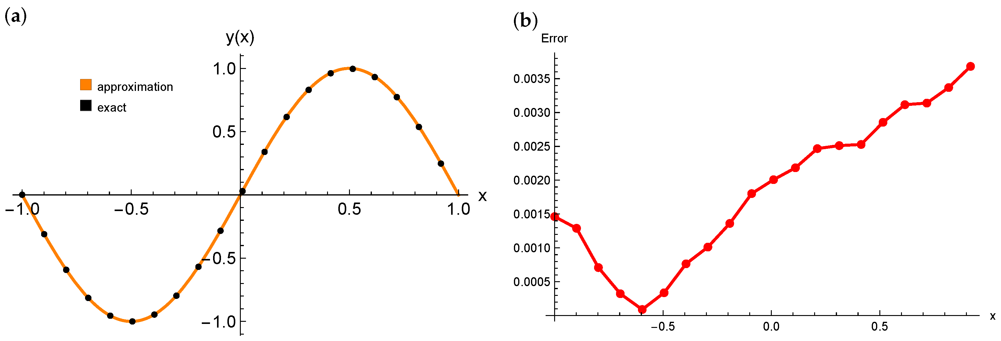
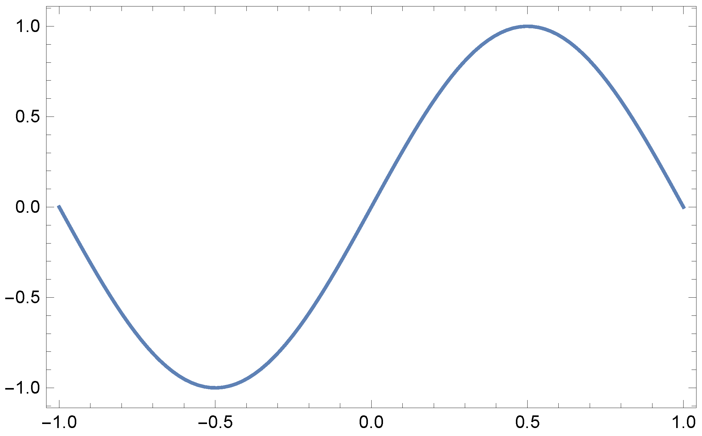
Figure 2 compares the PINNs solution with the exact solution, showcasing the network’s ability to closely match the theoretical result. The close alignment between the predicted and exact solutions confirms the robustness of PINNs for this class of problems. A plot of the absolute error as a function of x reveals that the error is expected to be minimal across the domain.

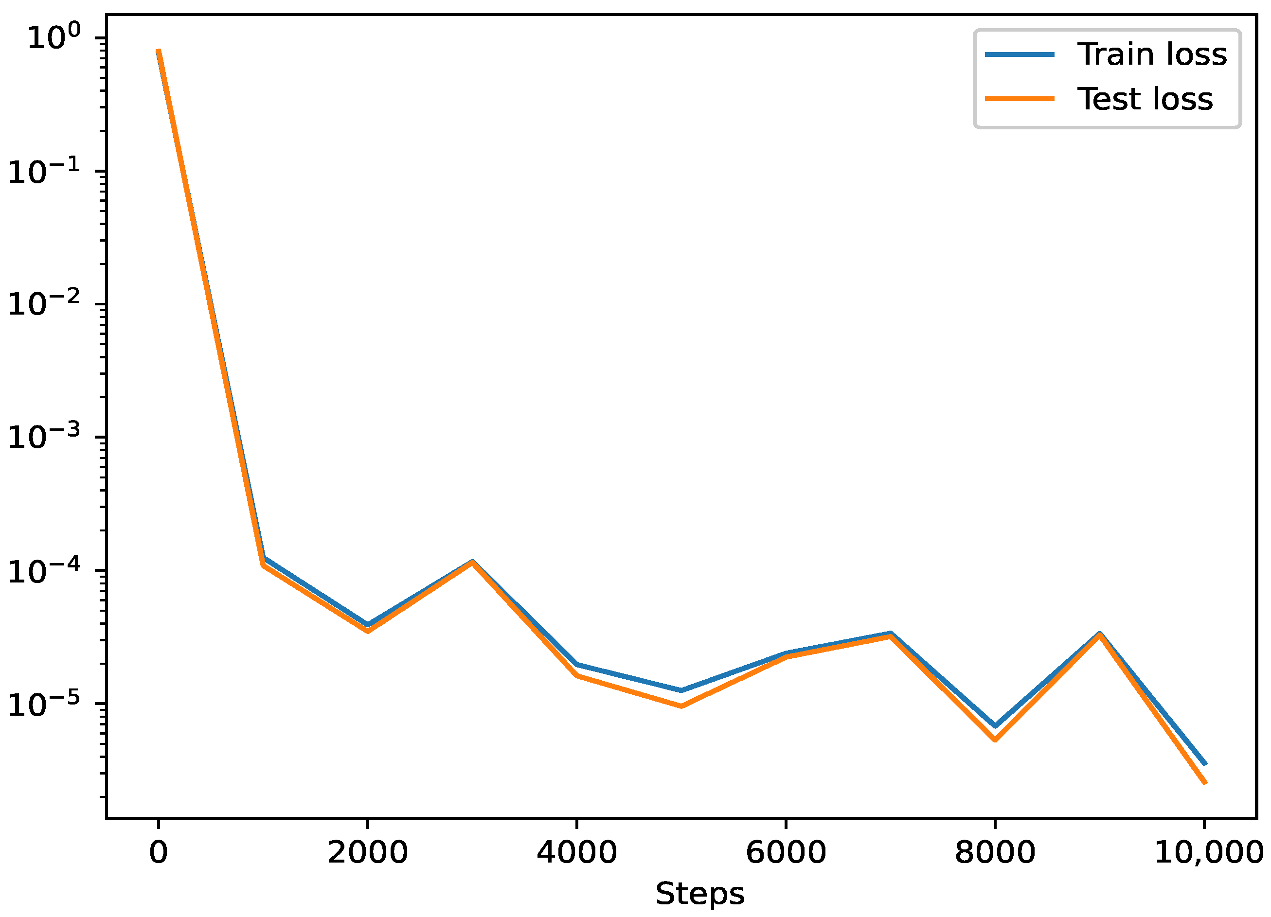
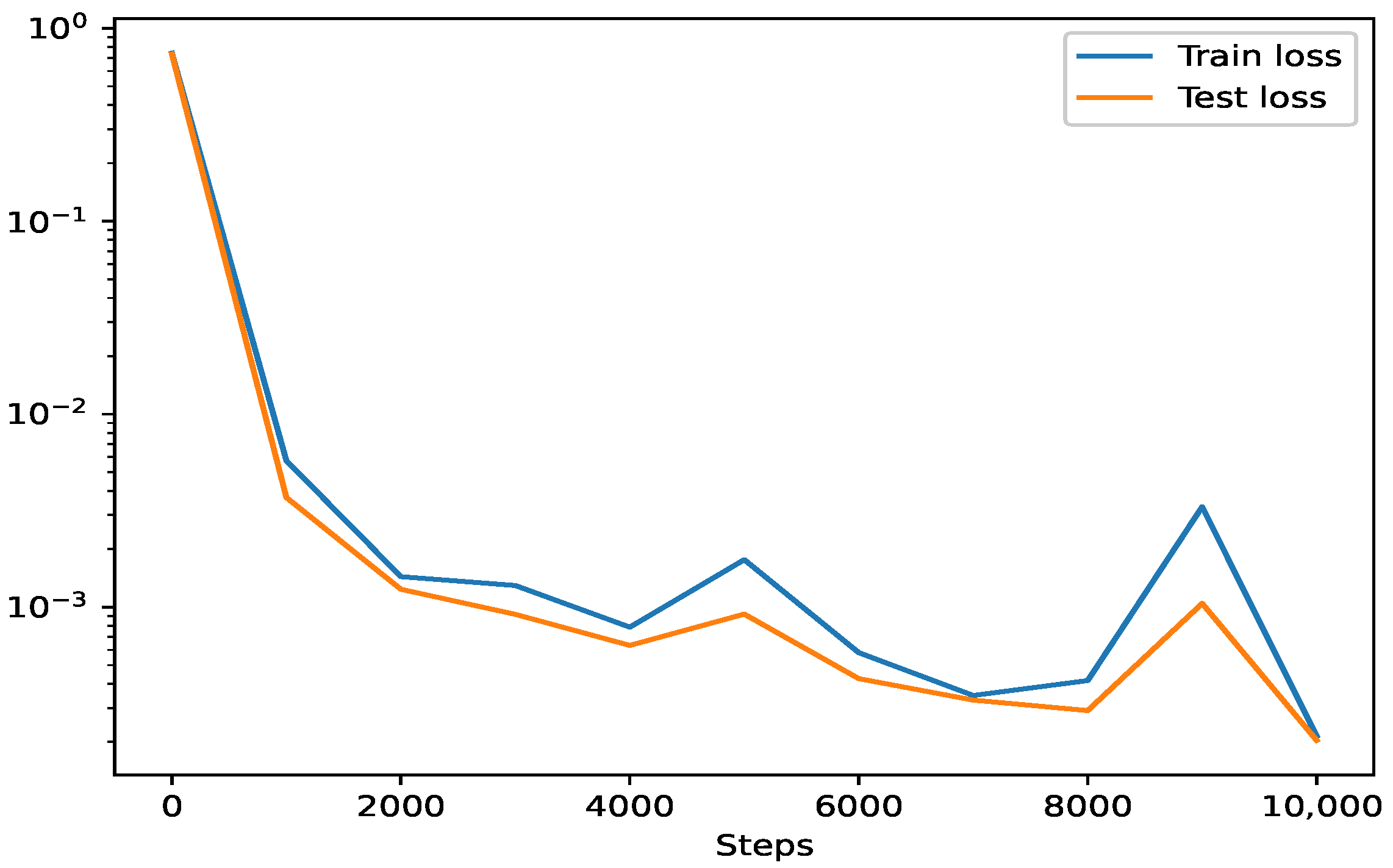
The train loss and test loss during the process of solving Equation (2) is shown in Figure 3. It can be seen that the training loss and test loss exhibit a strong correlation, with both decreasing sharply in early steps before stabilizing. The minimal gap between training and test loss highlights the model’s balanced capacity.

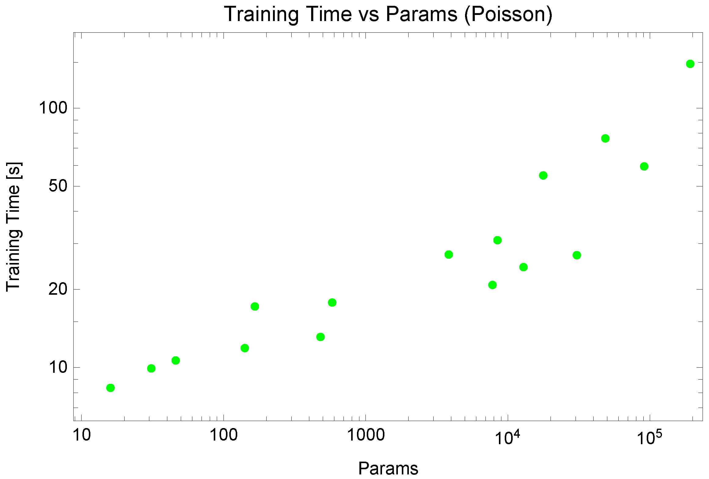
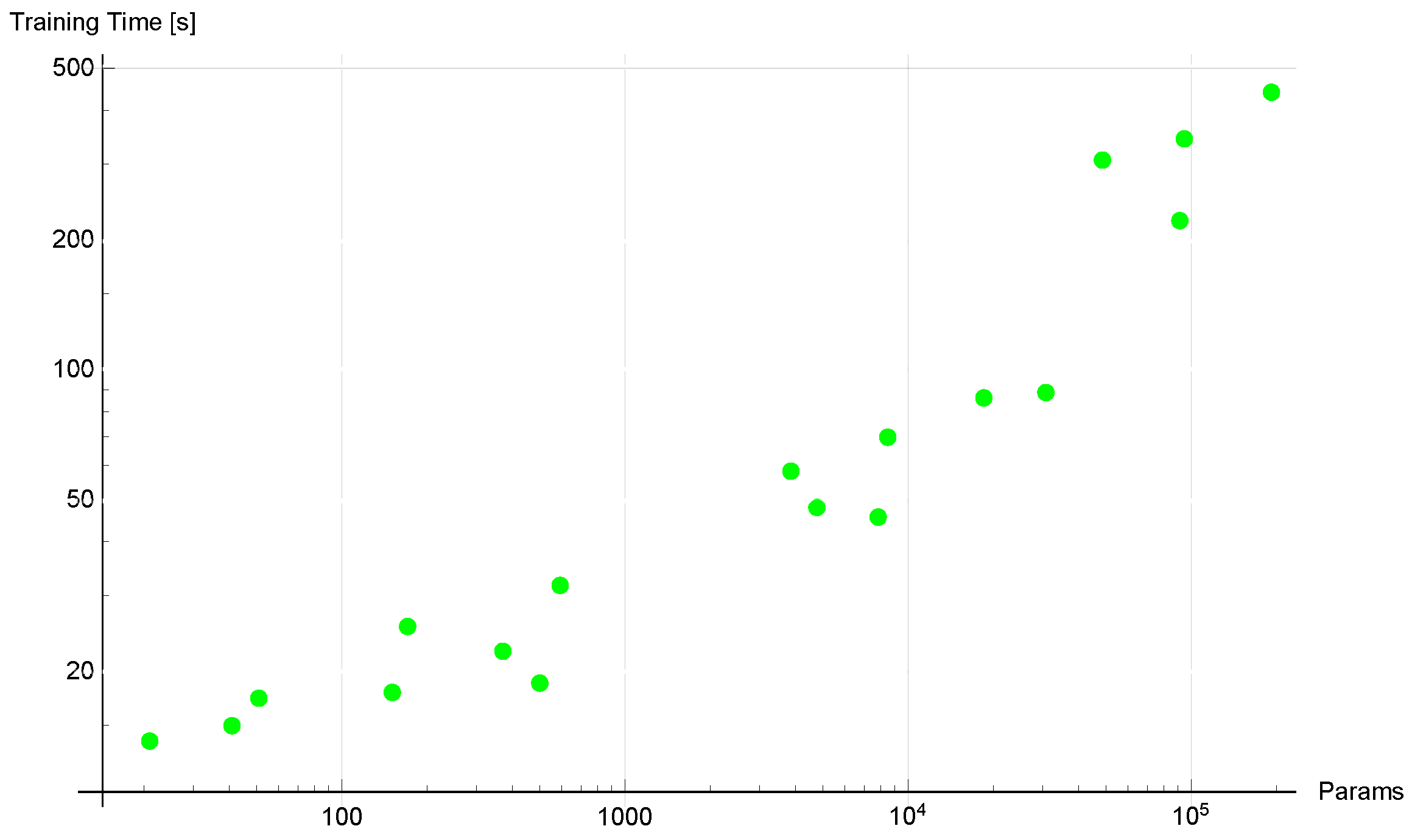
The influence of the number of hidden layers and neurons on the mean and maximum errors was also investigated. These errors were computed on a uniform test grid of dimension 100, independent of the training data. In all experiments, 200 collocation points and $10,000$ iterations were used. The last column in

Table 2. Performance of different hyperparameter combinations for Poisson equation.

Neurons	Hidden Layers	Mean Error	Max Error	Training Time [s]	Params
5	1	0.0000962	0.0004039	8.35	16
10	1	0.0002057	0.0004992	9.92	31
5	2	0.0000971	0.0002125	10.65	46
10	2	0.0002535	0.0007126	11.88	141
20	2	0.0000545	0.0001862	13.12	481
50	4	0.0012889	0.0023040	20.81	7801
100	4	0.0033755	0.0063511	27.10	30,601
5	6	0.0000933	0.0002061	17.19	166
10	6	0.0013967	0.0028064	17.80	581
50	6	0.0042395	0.0137589	24.37	12,901
20	10	0.0132887	0.0235891	27.25	3841
30	10	0.0041084	0.0084747	30.95	8461
100	10	0.0120098	0.0292455	59.57	91,201
30	20	0.0023960	0.0056850	54.97	17,761
50	20	0.0149564	0.0352005	76.35	48,601
100	20	0.0183402	0.0355639	147.95	192,201

(Params) refers to the total number of network parameters (weights and biases). The tests showed that the training time increases almost linearly with the number of parameters (correlation coefficient $\approx 0.95$). The lowest mean and maximum errors were obtained for moderately small architectures, e.g., $2\times 20$ (20 neurons, two hidden layers, $4.81\times {10}^2$ parameters). These networks achieved errors on the order of ${10}^{-4}$ with relatively short computation time (≈13 s). For very large architectures (e.g., $20\times 100$ with $192,201$ parameters), the results were significantly worse, with errors reaching the range of ${10}^{-2}$. This indicates optimization difficulties and instability of PINNs in this regime, likely due to the limited number of iterations (all tests used $10,000$ iterations). The best trade-offs between accuracy and training time are achieved by shallower and moderately wide networks, e.g., $2\times 20$ or $6\times 5$. Based on the data in Table 2, Figure 4 and Figure 5 illustrate the mean error as a function of the number of network parameters, as well as the computation time as a function of the number of parameters.

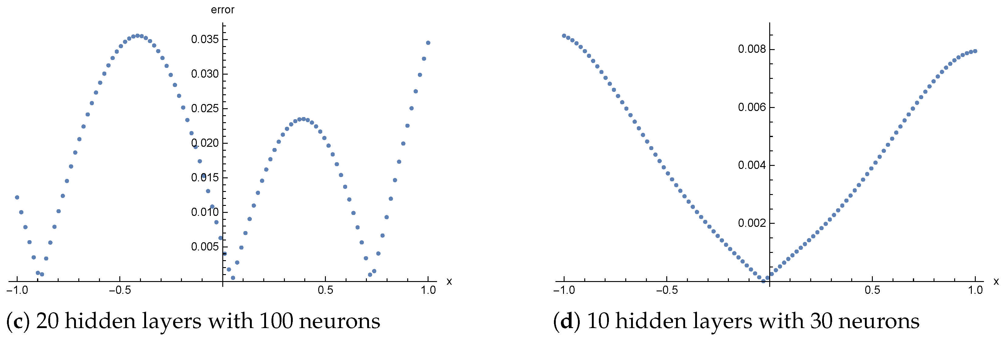
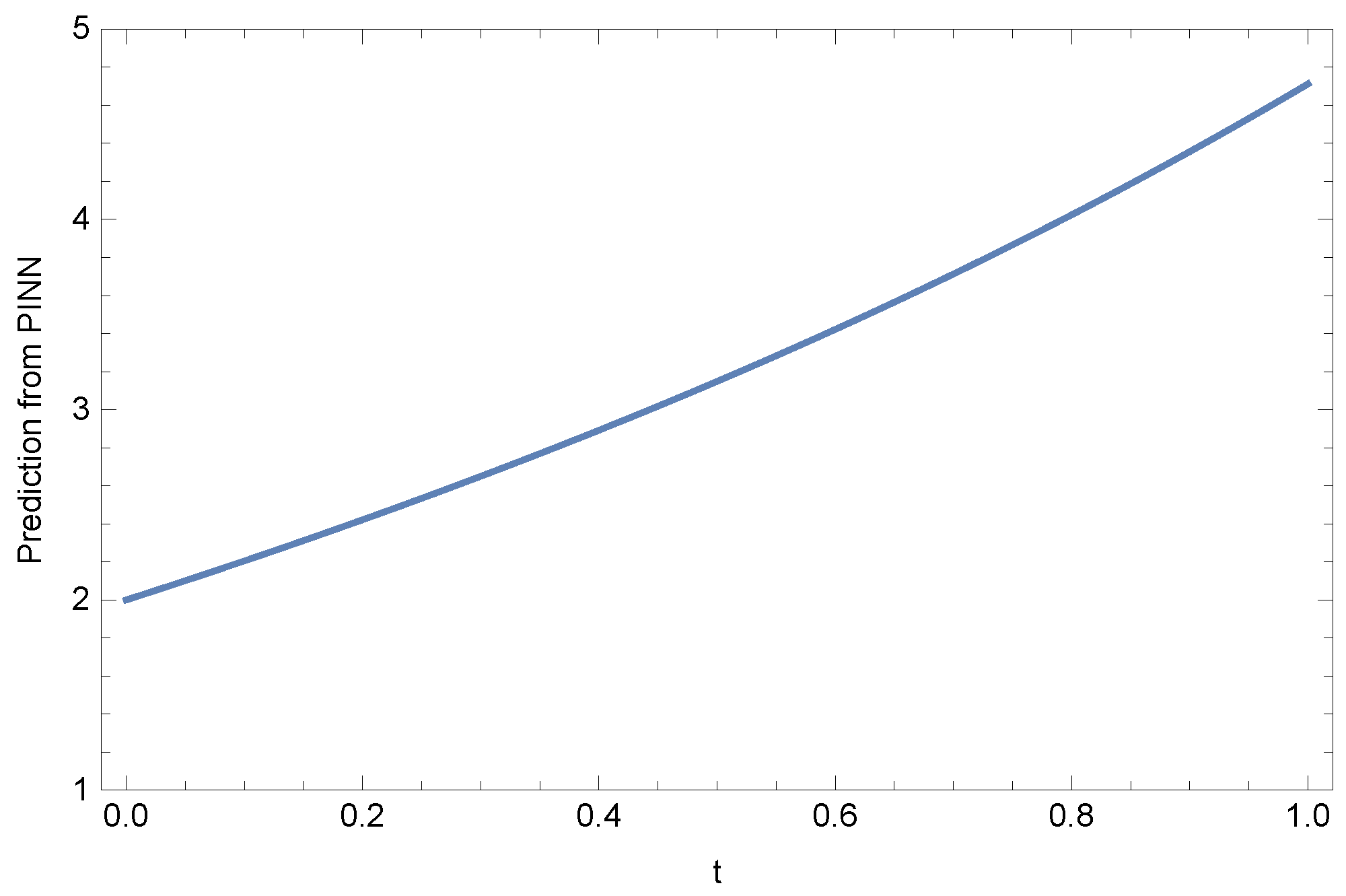
In Figure 6, the error distribution at the grid points is shown for four selected network architectures, while Figure 7 shows prediction from PINN for two hidden layers and 20 neurons.

The results, summarized in

Table 3. Mean and maximum error for different numbers of training points in the Poisson equation experiment.

Training Points	Mean Error	Max Error
100	0.0000069	0.0000126
500	0.0000030	0.0000067
1000	0.0000022	0.0000053
5000	0.0000013	0.0000037
10,000	0.0000011	0.0000022

, confirm the expected trend that the mean error decreases as the number of training points increases, thus providing numerical evidence for the theoretical convergence. We note, however, that simply increasing the number of training points is not sufficient by itself. To achieve stable convergence, it is also necessary to appropriately adjust the training procedure, in particular the number of iterations and the learning rate schedule of the Adam optimizer. Our experiments implement such a multi-stage training scheme, ensuring that the optimizer has the capacity to effectively use the additional information provided by more collocation points. In the cases of 5000 and 10,000 training points (compared to the other cases), the number of training iterations was significantly increased.

Additional experiments on the Poisson equation were conducted using several commonly employed activation functions, including ReLU, Sigmoid, sin, Swish, tanh, and ELU. The results are summarized in

Table 4. Mean and maximum error for different activation functions in the Poisson equation experiment.

Activation	Mean Error	Max Error
ReLU	0.6331564	0.9996860
Sigmoid	0.0000459	0.0000838
sin	0.0000770	0.0001597
Swish	0.0000285	0.0000698
tanh	0.0000158	0.0000494
ELU	0.0045412	0.0107337

. The comparison clearly shows that tanh yields the lowest errors among the tested functions, with Swish and Sigmoid also performing competitively well. In contrast, ReLU and ELU result in significantly larger prediction errors, confirming that smoother nonlinearities are more suitable for this PDE problem. These results justify our choice of tanh as the primary activation function in the paper, while also highlighting the potential of Swish and Sigmoid as alternatives in related applications.

3.2. Burgers’ Equation

Burgers’ equation is a fundamental partial differential equation (PDE) that combines nonlinear advection and diffusion, serving as a simplified model for fluid dynamics, shock waves, and traffic flow [33]. Burgers’ equation is a one-dimensional analog of the Navier–Stokes equations, making it a valuable tool for studying. It is given by the following:

$${\displaystyle \frac{\partial u}{\partial t}}+u{\displaystyle \frac{\partial u}{\partial x}}=\nu {\displaystyle \frac{{\partial }^{2}u}{\partial x^2}},a\le x\le b,t\ge 0$$

(3)

with boundary conditions and initial condition $u(a,t)=f\left(t\right),u(b,t)=g\left(t\right)$ and $u(x,0)=\varphi \left(x\right)$. In this case:

• u is the solution as a function of space and time, $u(x,t)$;
• $\nu$ is the viscosity coefficient which controls the smoothness of the solution;
• $f,g$ and $\varphi$ are known functions.

Burgers’ equation has its basis in the mathematical literature as shown by S.-S. Xie et al., who solved it using reproducing kernel function [34], and B. Inan et al., who solved it using implicit and fully implicit exponential finite difference methods [35]; even more extensive literature on Burgers’ equation can be seen in the work of M.P. Bonkile [36].

In this work we consider Equation (3) for $\nu =1$ with the initial condition

$$u(x,0)=sin\left(\pi x\right),0<x<1$$

and homogeneous boundary conditions

$$u(0,t)=u(1,t)=0,t>0.$$

This equation is solved by S. Kutluay et al. in [37]. They have used the explicit and exact-explicit finite difference methods to solve the equation with two different initial conditions. We explain the explicit and exact-explicit finite difference methods here and then compare the results through these methods with the physics-informed neural networks. First, we briefly describe these methods, and then we proceed with the comparison of the results.

3.2.1. Explicit Finite Difference Method

In this approach, the Burgers’ equation is discretized using a standard explicit scheme applied to the linear heat equation obtained via the Hopf–Cole transformation. The spatial domain $[0,1]$ is divided into N intervals with step size h, and the time domain is discretized with step size k. The finite difference approximation for the linear heat equation is given by the following:

$${\theta }_{i,j+1}=(1-2r){\theta }_{i,j}+r({\theta }_{i-1,j}+{\theta }_{i+1,j}),i=1,\dots ,N-1,$$

where $r={\displaystyle \frac{kv}{h^2}}$ and ${\theta }_{i,j}$ approximates the solution at grid point $(x_i,t_j)$. The boundary conditions are handled separately for $i=0$ and $i=N$. The stability condition for this method is $k\le {\displaystyle \frac{h^2}{2v}}$. Once the solution ${\theta }_{i,j}$ is computed, the Hopf–Cole transformation is applied to obtain the numerical solution for the Burgers’ equation:

$$u(x_i,t_j)=-{\displaystyle \frac{v}{h}}\left({\displaystyle \frac{{\theta }_{i+1,j}-{\theta }_{i-1,j}}{{\theta }_{i,j}}}\right).$$

This method is straightforward but requires careful attention to the stability constraint, especially for small values of viscosity $\nu$.

3.2.2. Exact-Explicit Finite Difference Method

This approach derives an exact solution to the finite difference scheme itself, rather than discretizing the continuous equation. The method assumes a product solution of the form ${\theta }_{i,j}=f_i{g}_j$, separating spatial ($f_i$) and temporal ($g_j$) components. The spatial part yields the following:

$$f_i=Bcos\left({\displaystyle \frac{is\pi }{N}}\right),s=0,1,2,...$$

while the temporal part satisfies the following:

$$g_j=A{\left(1-4r{sin}^2\left({\displaystyle \frac{s\pi }{2N}}\right)\right)}^j.$$

The complete solution combines these through superposition:

$${\theta }_{i,j}=\sum _{s=0}^{\infty }{D}_s{\left(1-4r{sin}^2\left({\displaystyle \frac{s\pi }{2N}}\right)\right)}^{j}cos\left({\displaystyle \frac{is\pi }{N}}\right).$$

The coefficients $D_s$ are determined from the initial condition using Fourier cosine series. Finally, the Hopf–Cole transformation converts this to the Burgers’ equation solution:

$$u(x_i,t_j)=2\pi v{\displaystyle \frac{{\sum }_{s=1}^{\infty }{D}_s\left(1-4r{sin}^2{\left(\frac{s\pi }{2N}\right)}^{j}ssin\left(s\pi x_i\right)\right)}{D_0+{\sum }_{s=1}^{\infty }{D}_s{\left(1-4r{sin}^2\left(\frac{s\pi }{2N}\right)\right)}^{j}cos\left(s\pi x_i\right)}}.$$

This method provides an exact solution to the discrete equations, converging to the Fourier solution as $h\to 0$.

3.2.3. Accuracy Comparison Between Classical Numerical Methods and PINNs

We have solved Equation (3) using PINNs and then compare the results with the results obtained from explicit, exact-explicit methods, and with exact solution [37]. The solutions are obtained using 200 training points and 10 layers of neurons, each with five neurons, while the activation function is tanh.

Table 5. Comparison of numerical solutions using explicit method, exact-explicit method, and PINNs with exact solution at $t=0.1$ and $v=1$.

x	Explicit [37]	Exact-Explicit [37]	PINNs	Exact Solution
0.1	0.10863	0.11048	0.11166	0.10954
0.2	0.20805	0.21159	0.21210	0.20979
0.3	0.28946	0.29435	0.29440	0.29190
0.4	0.34501	0.35080	0.35059	0.34792
0.5	0.36845	0.37458	0.37446	0.37158
0.6	0.35601	0.36189	0.36214	0.35905
0.7	0.30728	0.31231	0.31310	0.30991
0.8	0.22588	0.22955	0.23133	0.22782
0.9	0.11966	0.12160	0.12559	0.12069

shows a comparison of numerical solutions obtained using the explicit method, exact-explicit method, and PINNs with the exact solution at time $t=0.1$ and $\nu =1$. We can see that all methods closely follow the exact solution, but there are small differences. The PINNs method gives values that are very close to the exact solution, especially at points where x is around $0.5$.

A comparison of exact solution and approximate solutions is given in Figure 8. Figure 8a plots these solutions visually. The PINNs, Explicit, and Exact-Explicit solutions all follow the exact solution curve very well. However, the small differences are more noticeable in Figure 8b, which shows the absolute error between each method and the exact solution. The Explicit method has the largest error near $x=0.5$, while PINNs and Exact-Explicit methods have smaller and more consistent errors.

Figure 9 shows the training and testing loss of the PINNs model. Both the training and testing losses decrease quickly in the first few steps and continue to go down gradually. This suggests that the model is learning well and generalizing properly without overfitting.

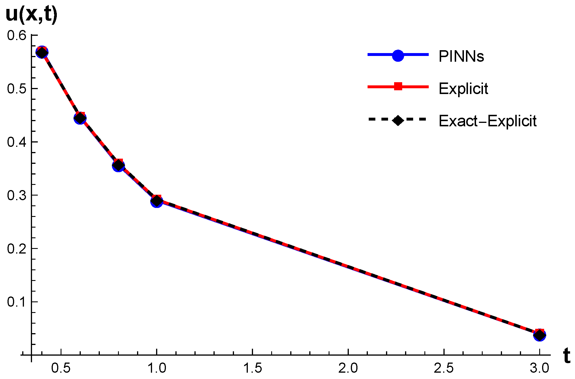
To further validate the performance of the physics-informed neural networks approach in solving Burgers’ equation, we investigated the evolution of the solution at a fixed spatial point $x=0.5$.

Table 6. Comparison of the numerical solutions with exact solution at different times for $v=0.1$.

x	t	Numerical Solution			Exact Solution
		Explicit [37]	Exact-Explicit [37]	PINNs
0.5	0.4	0.56911	0.56964	0.57055	0.56963
	0.6	0.44676	0.44721	0.44644	0.44721
	0.8	0.35888	0.35924	0.35721	0.35924
	1.0	0.29162	0.29192	0.29031	0.29192
	3.0	0.04017	0.04021	0.04003	0.04021

presents a comparison between the PINNs solution and traditional numerical methods (explicit and exact-explicit schemes) against the exact solution for various time values. It is evident from the table that the PINNs approach provides results with high accuracy, closely matching the exact solution.

As time progresses from $t=0.4$ to $t=3.0$, the solution $u(x,t)$ exhibits a smooth decay, which is characteristic of the dissipative nature of Burgers’ equation with viscosity $\nu =0.1$. This behavior is clearly illustrated in Figure 10, where the PINNs prediction aligns tightly with both explicit schemes and the exact solution.

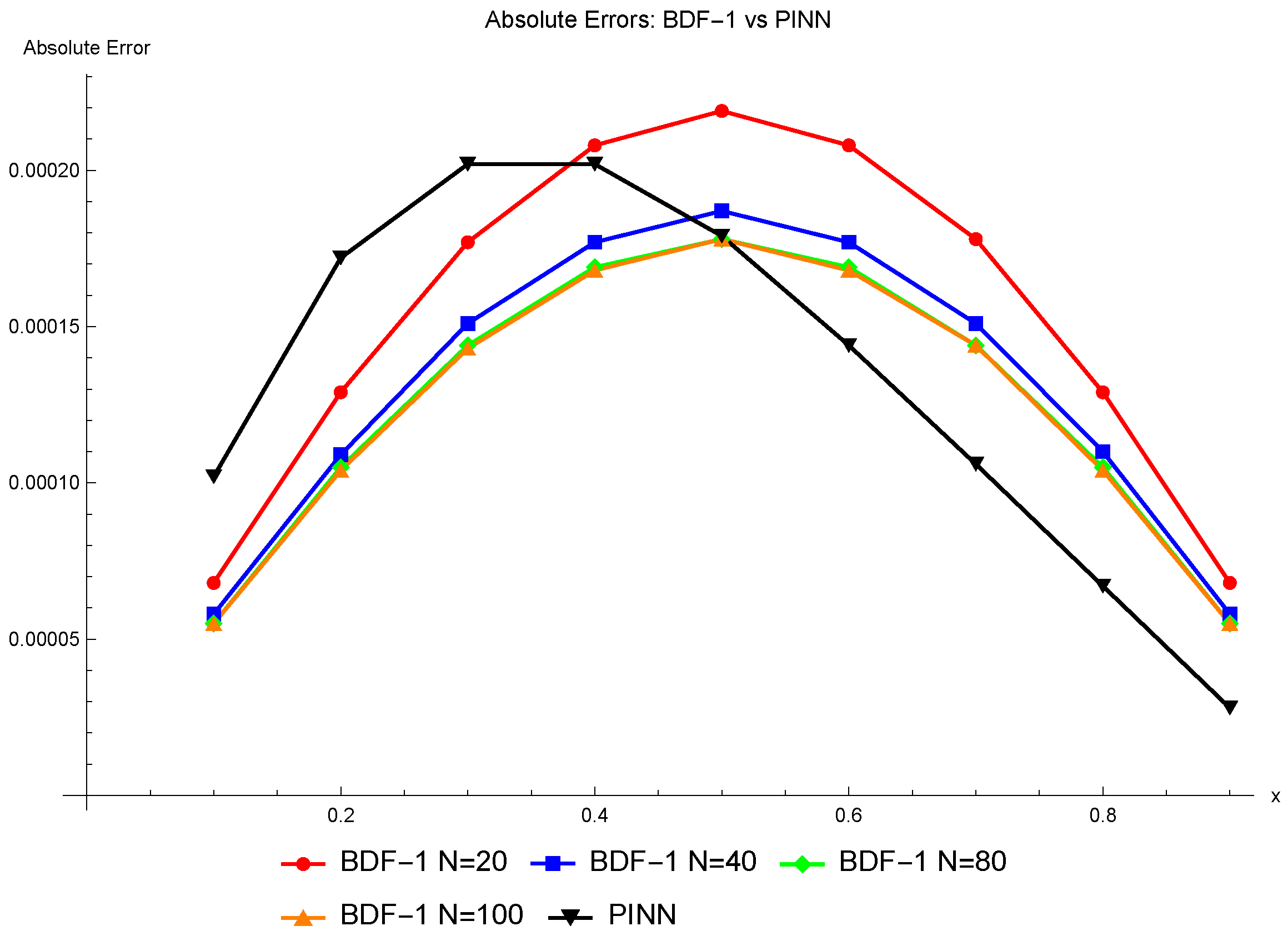
As part of the tests, a comparison was also conducted with another numerical method described in [38]. This method depends on the mesh density (parameter N).

Table 7. Comparison of the numerical solution (BDF-1) with the exact solution and PINN method at different space points for $t=0.5$.

x	$\mathit{N}=20$	$\mathit{N}=40$	$\mathit{N}=80$	$\mathit{N}=100$	Exact Solution	PINN
0.1	2.281 × 10−3	2.271 × 10−3	2.268 × 10−3	2.268 × 10−3	2.213 × 10−3	2.315 × 10−3
0.2	4.339 × 10−3	4.319 × 10−3	4.315 × 10−3	4.314 × 10−3	4.210 × 10−3	4.382 × 10−3
0.3	5.973 × 10−3	5.947 × 10−3	5.940 × 10−3	5.939 × 10−3	5.796 × 10−3	5.998 × 10−3
0.4	7.024 × 10−3	6.993 × 10−3	6.985 × 10−3	6.984 × 10−3	6.816 × 10−3	7.018 × 10−3
0.5	7.388 × 10−3	7.356 × 10−3	7.347 × 10−3	7.347 × 10−3	7.169 × 10−3	7.348 × 10−3
0.6	7.029 × 10−3	6.998 × 10−3	6.990 × 10−3	6.989 × 10−3	6.821 × 10−3	6.965 × 10−3
0.7	5.982 × 10−3	5.955 × 10−3	5.948 × 10−3	5.948 × 10−3	5.804 × 10−3	5.910 × 10−3
0.8	4.347 × 10−3	4.328 × 10−3	4.323 × 10−3	4.322 × 10−3	4.218 × 10−3	4.285 × 10−3
0.9	2.286 × 10−3	2.276 × 10−3	2.273 × 10−3	2.273 × 10−3	2.218 × 10−3	2.246 × 10−3

presents the values obtained with the referenced numerical method, the results from PINN, as well as the exact solutions. Figure 11 shows the error plots for the referenced method (for $N=20,40,80,100$) and for the PINN results at $t=0.5$. The errors of the PINN solution are comparable to those reported in [38]. However, it can be observed that for $x>0.5$, the errors obtained with PINN are smaller.

Another test involved examining how the weights in the loss function on the PDE and the initial–boundary conditions affected the obtained results. For this purpose, a set of several weights was assumed, and after training the model, the mean error computed on a $100\times 100$ grid was evaluated (see

Table 8. The effect of loss function weights on the mean and maximum error of the results.

Weights $({\mathit{\lambda }}_{\mathit{PDE}},{\mathit{\lambda }}_{\mathit{IC}},{\mathit{\lambda }}_{{\mathit{BC}}_{\mathit{left}}},{\mathit{\lambda }}_{{\mathit{BC}}_{\mathit{right}}})$	Mean Error	Max Error
(5.0, 1.0, 1.0, 1.0)	0.0126755	0.0766495
(1.0, 5.0, 1.0, 1.0)	0.00730921	0.0546295
(1.0, 1.0, 5.0, 5.0)	0.00579474	0.0411806
(10.0, 1.0, 1.0, 1.0)	0.0111069	0.103218
(1.0, 10.0, 10.0, 10.0)	0.00258062	0.0196944
(1.0, 5.0, 5.0, 5.0)	0.00197403	0.0177932

). In this test, the network architecture and hyperparameters were as follows: hidden layers: 5; neurons per layer: 10; Adam optimizer; collocation points inside domain: 200; boundary/initial condition points: 128; number of iterations: 10,000. It is also assumed that $x,t\in [0,1]$.

The weights assigned to individual components of the loss function have a moderate impact on the obtained errors. In particular, it can be clearly observed that when the weights for the initial–boundary conditions are several times larger than those for the PDE inside the domain, the resulting solution errors are significantly reduced.

The effect of the distribution of collocation points on the mean and max errors in the domain, computed on a $100\times 100$ grid, was also examined (see

Table 9. Effect of collocation point distribution type on the mean and maximum error.

Collocation Point Distribution Type	Mean Error	Max Error
uniform (equispaced grid)	0.00511845	0.0278437
pseudo (pseudorandom)	0.00418709	0.029266
LHS (Latin hypercube sampling)	0.00696592	0.0361623
Halton (Halton sequence)	0.00759538	0.0478001
Hammersley (Hammersley sequence)	0.00372326	0.0329703
Sobol (Sobol sequence)	0.00485239	0.0341695

). The impact of the number of collocation points inside domain on this error was also investigated (see

Table 10. Effect of the number of collocation points on the mean and maximum error.

Number of Collocation Points	Mean Error	Max Error	Time of Training Model [s]
50	0.00541526	0.0308579	25.12
100	0.00516718	0.0317111	28.76
500	0.00630318	0.0403584	31.06
1000	0.00418513	0.0254188	34.44
10,000	0.00140849	0.0123031	120.84

). In these tests, equal weights were used, while the settings of the remaining parameters and the network architecture are the same as in the previous test.

The differences in the obtained errors when changing the distribution of collocation points are minor. The smallest errors were obtained using the Hammersley method. When increasing the number of collocation points, the obtained errors were slightly smaller. For example, taking 10,000 points results in the max error $\approx 0.012$, while for 100 points it was ≈0.031. However, even with 50 points, the results are satisfactory. Increasing the number of collocation points only slightly reduces the errors while extending the computation time. Additionally, the training times of the model are provided in Table 10. Increasing the number of collocation points leads to longer computation times; however, the growth is not linearly proportional. For example, for 1000 collocation points, the computation time was 34 s, whereas for 10,000 points, the model required approximately 120 s to train.

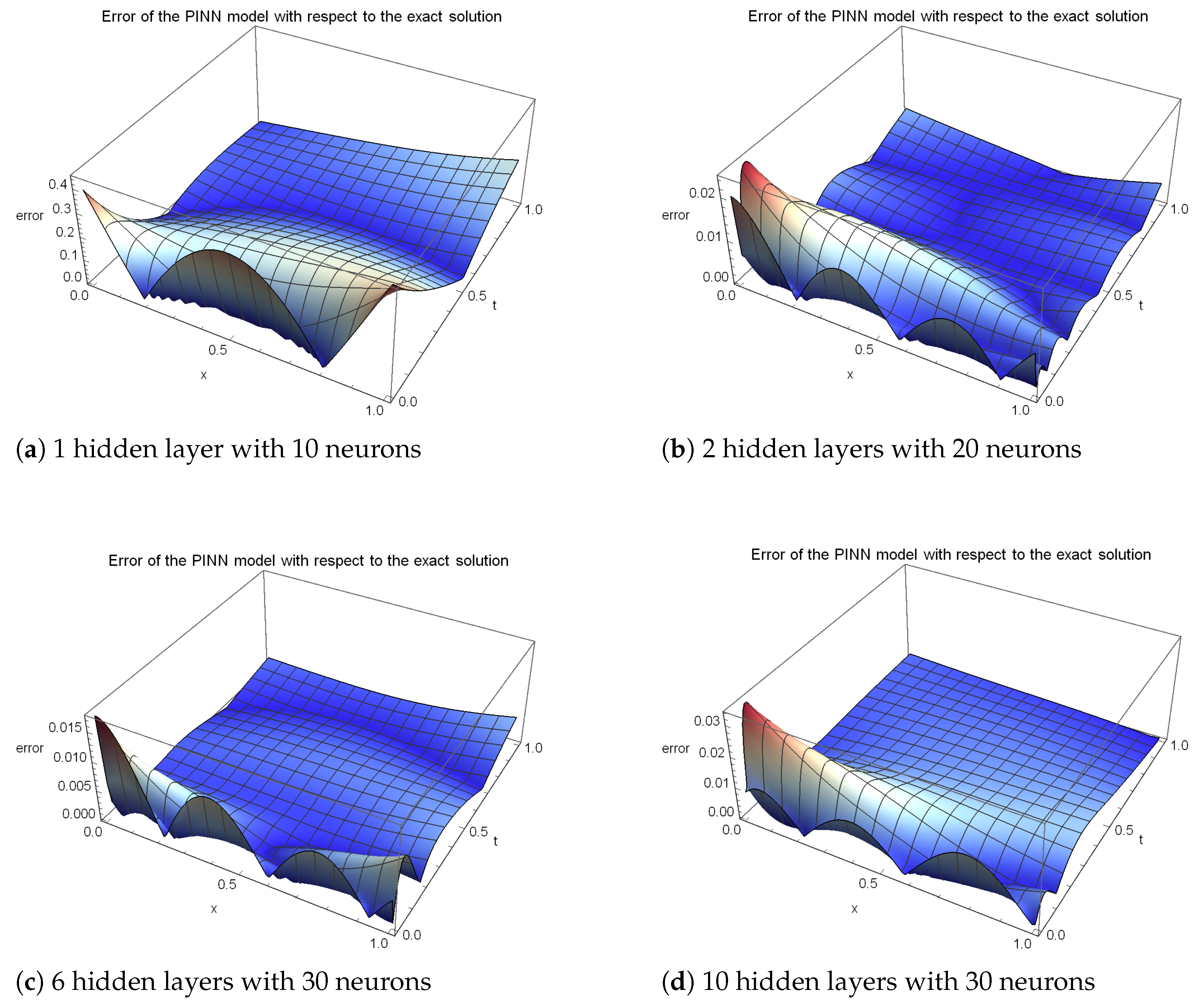
The final test conducted on this example was to examine the impact of the network architecture (the number of hidden layers and neurons per layer) on the obtained errors. The results of this test are shown in

Table 11. Performance of different hyperparameter combinations concerning number of hidden layers and neurons.

Neurons	Hidden Layers	Mean Error	Max Error	Training Time [s]	Params
5	1	0.0666834	0.436997	13.79	21
10	1	0.0969972	0.445789	14.97	41
5	2	0.0229704	0.147473	17.33	51
10	2	0.0037768	0.045616	17.88	151
20	2	0.0030077	0.024509	18.79	501
10	4	0.0044155	0.035810	22.28	371
50	4	0.0055573	0.029546	45.59	7851
100	4	0.0110681	0.020511	88.62	30,701
5	6	0.0141401	0.084471	25.42	171
10	6	0.0029999	0.018322	31.66	591
30	6	0.0018869	0.017416	48.00	4771
60	6	0.0119612	0.058198	86.14	18,541
20	10	0.0049465	0.024834	58.23	3861
30	10	0.0059858	0.033673	69.82	8491
100	10	0.0050738	0.059602	221.90	91,301
50	20	0.0052591	0.034503	306.45	48,651
70	20	0.0343433	0.0484721	343.27	94,711
100	20	0.0089822	0.0848633	440.17	192,301

. The last column in Table 11, named Params, refers to the total number of network parameters (the number of weights and biases). An insufficient number of hidden layers or neurons in the network is not enough for the model to provide satisfactory predictions. The mean and maximum errors for a single hidden layer are unsatisfactory, as are the errors for two hidden layers with five neurons. Moving from one to two layers yields the largest quality jump (e.g., with 10 neurons Mean Error drops $0.097$ to $0.0038$ at similar training time). The best results were obtained with six layers and 30 neurons. Increasing the number of hidden layers and neurons has a significant impact on the computation time. The training time grows almost linearly with the number of parameters (correlation $\approx 0.93$). Large and deep models may require significantly longer training time without a guaranteed improvement in error. The results indicate that some deeper yet still moderately wide models (e.g., $6\times 30$) are more efficient per parameter and per unit of time than very wide ones (e.g., $10\times 100$, $20\times 100$), which suffer from optimization difficulties. Based on the data in the Table, Figure 12 and Figure 13 show the mean error as a function of the number of network parameters, as well as the computation time as a function of the number of parameters. The solution obtained from PINN for best case is presented in Figure 14. Figure 15 shows the error distribution obtained from the PINN model for selected network architecture settings. The smallest errors were obtained with six hidden layers and 30 neurons (Figure 15c), while the largest errors occurred with one hidden layer and 10 neurons (Figure 15a).

The results demonstrate that physics-informed neural networks (PINNs) can effectively solve the Burgers’ equation with high accuracy as compared to traditional methods like the explicit and exact-explicit schemes. PINNs produced smaller approximation errors across most of the domain.

3.3. Volterra Integro-Differential Equation

Volterra integro-differential equations (VIDEs) are a class of functional equations that combine differential and integral operations on an unknown function. A standard form of a first-order VIDE is as follows:

$${\displaystyle \frac{d}{dt}}y\left(t\right)=f\left(t,y\left(t\right)\right)+{\int }_0^{t}K(t,s,y\left(s\right))ds,$$

where $K(t,s,y(s\left)\right)$ is a known kernel function, and f defines the local dynamics. VIDEs naturally arise in systems where the future state depends not only on the current state but also on the historical evolution of the system [39].

Volterra integro-differential equations appear in various scientific and engineering contexts such as population dynamics, heat transfer in materials with memory, neuroscience, finance, etc. A detailed analysis and overview on these models can be seen in the works [40,41]. Thus, these equations are crucial for modeling systems where historical data fundamentally influences future dynamics.

Traditional numerical techniques, such as quadrature methods, finite difference schemes, or collocation methods, often face difficulties due to high computational cost from evaluating the integral term at each time step, stability issues over long time intervals, and accuracy demands for capturing both differential and integral contributions. These challenges intensify for higher-order VIDEs due to the presence of multiple derivatives and their interactions with history-dependent terms. PINNs offer a modern approach by embedding the physical laws into the loss function of a neural network.

In this section we are going to solve a fourth order Volterra integro-differential equation using PINNs and then compare the results with a traditional numerical method where the same equation is solved using variational iteration method with collocation. First we will describe this method and see its convergence analysis and then compare the results through figures and tables. The equation is solved by Otaide et al. in their work on “Numerical treatment of linear Volterra integro differential equations using variational iteration algorithm with collocation” [42]. The equation is described as

$$\left\{\begin{array}{cc}\hfill & y^{\left(iv\right)}\left(t\right)=1+t-{\displaystyle \frac{t^2}{2}}-{\displaystyle \frac{t^3}{6}}+{\int }_0^t(t-s)y\left(s\right)ds,\hfill \\ \hfill & y\left(0\right)=2,y^{\prime }\left(0\right)=2,y^{″}\left(0\right)=1,y^{‴}\left(0\right)=1.\hfill \end{array}\right.$$

(4)

The exact solution for this problem is as follows:

$$y\left(t\right)=exp\left(t\right)+t+1.$$

In the work of Otaide et al. [42], the equation is solved using fourth-kind Chebyshev polynomials combined with the variational iteration method and a collocation technique, resulting in a hybrid approach that integrates variational iteration with collocation. The method is briefly described in Section 3.3.1.

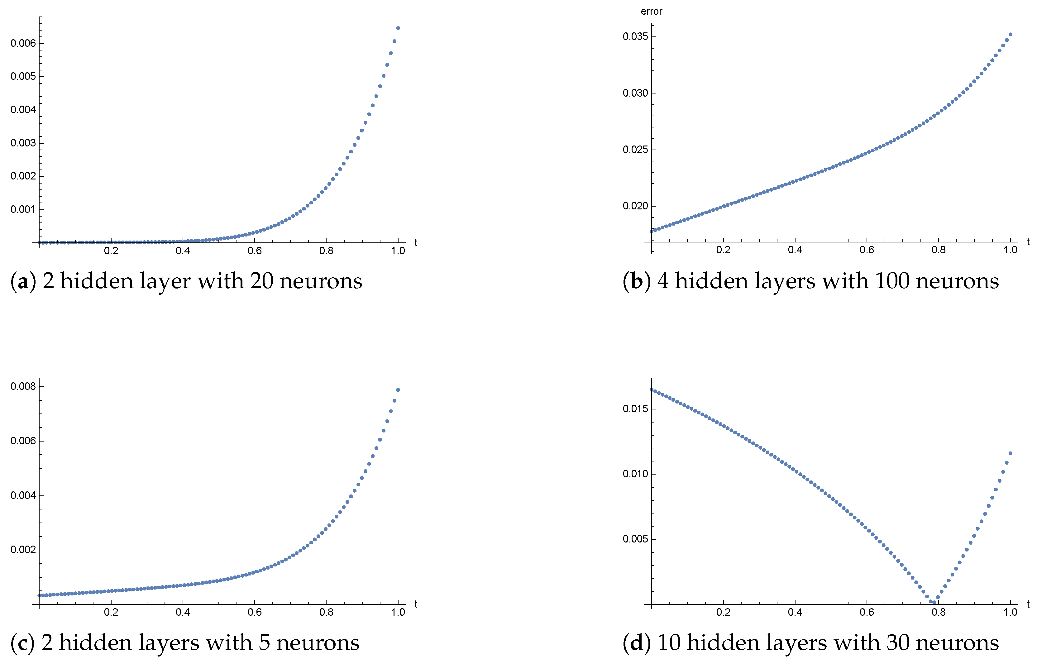
Before comparing the results obtained with PINNs to those from the method described in Section 3.3.1, computations were performed on various network architectures (see

Table 12. Performance of different hyperparameter combinations for VIDE.

Neurons	Hidden Layers	Mean Error	Max Error	Training Time [s]	Params
5	1	0.00111956	0.00684174	13.32	16
10	1	0.00102483	0.00675019	14.14	31
5	2	0.00174907	0.00788888	20.45	46
10	2	0.000961112	0.00644263	26.92	141
20	2	0.000949299	0.00646266	38.24	481
50	4	0.000996002	0.00644883	335.16	7801
100	4	0.0242298	0.0352155	706.06	30,601
5	6	0.00109214	0.00678214	129.42	166
10	6	0.00102154	0.00660905	314.78	581
50	6	0.000891232	0.00629672	663.80	12,901
20	10	0.0424468	0.0460251	1036.78	3841
30	10	0.00881867	0.016485	1168.29	8461
100	10	0.00157222	0.00746592	1870.17	91,201

). Similar to the previous examples, the lowest mean errors were achieved by moderate architectures: $2\times 20$ (Mean $=9.49\times {10}^{-4}$), $2\times 10$ (Mean $=9.61\times {10}^{-4}$), and $6\times 50$ (Mean $=8.91\times {10}^{-4}$). Analogous to the previously analyzed examples, Figure 16 presents the error distribution at the grid points for four sample cases from Table 12. The solution obtained with PINN using six hidden layers and 50 neurons is shown in Figure 17.

3.3.1. The Standard Variational Iteration Method Combined with Shifted Chebyshev Polynomials of the Fourth Kind

Consider a Volterra integro-differential equation of the form

$$y^{\left(n\right)}\left(t\right)=f\left(t\right)+{\int }_0^{t}K(t,s)y\left(s\right)ds,$$

(5)

where $y^{\left(n\right)}\left(t\right)$ is the unknown function, $f\left(t\right)$ is a known forcing term, and $K(t,s)$ is the kernel. The correction functional for Variational Iteration Method (VIM) is

$$y_{m+1}\left(t\right)=y_m\left(t\right)+{\int }_0^t\lambda \left(s\right)\left(y_m^{\left(n\right)}\left(s\right)-f\left(s\right)-{\int }_0^{s}K(s,\tau )y_m\left(\tau \right)d\tau \right)ds,$$

with $\lambda \left(s\right)$ as the Lagrange multiplier determined optimally using variational principles. The subscript m indicates the mth iteration, and $y_m\left(t\right)$ is considered as a restricted variation ($\delta y_m=0$) during the optimization.

To discretize the problem, we apply the standard collocation technique by choosing collocation points uniformly distributed over $[a,b]$

$$t_i=a+{\displaystyle \frac{(b-a)i}{N}},i=1,2,\dots ,N,$$

where N denotes the number of collocation points. This discretization converts the continuous problem into a system of algebraic equations.

For better approximation, we expand the solution using Chebyshev polynomials of the fourth kind $W_n\left(t\right)$, which are orthogonal with respect to the weight function

$$w\left(t\right)=\sqrt{{\displaystyle \frac{1-t}{1+t}}},t\in [-1,1].$$

These polynomials satisfy the recurrence relation

$$W_{n+1}\left(t\right)=2t{W}_n\left(t\right)-W_{n-1}\left(t\right),W_0\left(t\right)=1,W_1\left(t\right)=2t+1.$$

Chebyshev polynomials exhibit excellent approximation properties, such as rapid convergence and minimization of the maximum error.

To adapt Chebyshev polynomials to the interval $[0,1]$, we employ the shifted Chebyshev polynomials $W_n^{\ast }\left(t\right)$ defined by the following:

$$W_n^{\ast }\left(t\right)=W_n(2t-1),$$

with the following recurrence relation:

$$W_{n+1}^{\ast }\left(t\right)=2(2t-1)W_n^{\ast }\left(t\right)-W_{n-1}^{\ast }\left(t\right),W_0^{\ast }\left(t\right)=1,W_1^{\ast }\left(t\right)=4t-1.$$

These shifted polynomials retain the favorable properties of their unshifted counterparts while matching the domain of the problem. The hybrid method approximates the solution as

$$y_{m,N}\left(t\right)=\sum _{k=0}^{N-1}{c}_{k,N}{W}_k^{\ast }\left(t\right),$$

and iteratively refines it using

$$y_{m+1,N}\left(t\right)=\sum _{k=0}^{N-1}{c}_{k,N}{W}_k^{\ast }\left(t\right)+{\int }_0^t\lambda \left(s\right)\left({\displaystyle \frac{d^n{y}_{m,N}}{d{s}^n}}-f\left(s\right)-{\int }_0^{s}K(s,\tau )y_{m,N}\left(\tau \right)d\tau \right)ds,$$

where $c_{k,N}$ are coefficients to be determined.

3.3.2. Convergence of the Method

When solving a differential equation numerically using the iteration methods, it is important to prove that the method actually converges, i.e., the sequence of approximations $y_m\left(t\right)$ produced by the method will become closer and closer to the true solution as $m\to \infty$. This analysis—in this case—relies on the Banach’s Fixed-Point Theorem.

Theorem 5

Let X be a Banach space with norm $\parallel ·\parallel$, and let $\mathcal{F}:X\to X$ be the linear operator defined by the following:

$$\mathcal{F}\left[y\right]=y_{m,N}\left(t\right)+{\int }_0^t\lambda \left(s\right)\left({\displaystyle \frac{d^n{y}_m}{d{s}^n}}-f\left(s\right)-{\int }_0^{s}K(s,\tau )y_m\left(\tau \right)d\tau \right)ds,$$

where $y_{m,N}\left(t\right)={\sum }_{k=0}^{N-1}{c}_{k,N}{W}_k^{\ast }\left(t\right)$ is the approximate solution using shifted Chebyshev polynomials $W_k^{\ast }$. If $\mathcal{F}$ is a contraction, i.e., there exists $\zeta \in [0,1)$ such that

$$\parallel \mathcal{F}\left[y\right]-\mathcal{F}\left[\tilde{y}\right]\parallel \le \zeta \parallel y-\tilde{y}\parallel \forall y,\tilde{y}\in X,$$

then

1.

$\mathcal{F}$ has a unique fixed point $y^{\ast }\in X$.

2.

The sequence $\left\{y_{m,N}\right\}$ generated by $y_{m+1,N}=\mathcal{F}\left[y_{m,N}\right]$ converges to $y^{\ast }$ for any initial guess $y_{0,N}$.

Proof. 

By the Banach Fixed-Point Theorem, $\mathcal{F}$ has a unique fixed point $y^{\ast }$ since X is complete and $\mathcal{F}$ is a contraction. For $p>q\ge 1$, the triangle inequality and contraction property yield

$$\parallel y_p-y_q\parallel \le \sum _{k=q}^{p-1}\parallel y_{k+1}-y_k\parallel \le \left({\zeta }^q+\dots +{\zeta }^{p-1}\right)\parallel y_1-y_0\parallel .$$

The series converges as $\zeta <1$, so $\left\{y_{m,N}\right\}$ is Cauchy and thus convergent. At the fixed point $y^{\ast }$, the iteration reduces to

$$y^{\ast }\left(t\right)=y^{\ast }\left(t\right)+{\int }_0^t\lambda \left(s\right)\left({\displaystyle \frac{d^n{y}^{\ast }}{d{s}^n}}-f\left(s\right)-{\int }_0^{s}K(s,\tau )y^{\ast }\left(\tau \right)d\tau \right)ds,$$

implying ${\displaystyle \frac{d^n{y}^{\ast }}{d{t}^n}}=f\left(t\right)+{\int }_0^{t}K(t,\tau )y^{\ast }\left(\tau \right)d\tau$. Hence, $y^{\ast }$ solves the VIDE. □

Proposition 1.

According to Theorem 5, for the linear mapping $\mathcal{F}$ defined as the following:

$$\mathcal{F}\left[y\right]=y_{m,N}\left(t\right)+{\int }_0^t\lambda \left(t\right)(L{y}_m\left(t\right)+N\widetilde{y_m\left(t\right)}-g\left(t\right))dt$$

or equivalently

$$\mathcal{F}\left[y\right]=\sum _{m=0}^N{c}_{m,N}{W}_{m,N}^{\ast }\left(t\right)+{\int }_0^t\lambda \left(t\right)\left({\displaystyle \frac{d^{n}y}{d{s}^n}}-f\left(s\right)-{\int }_0^{t}K(s,t)y\left(t\right)dt\right)ds,$$

this is a necessary condition for the variational iteration approach to converge. The sequence $y_{n+1}=\mathcal{F}\left[y_n\right]$ converges to a fixed point of $\mathcal{F}$ which is also a solution of (5).

3.3.3. Comparison of Results

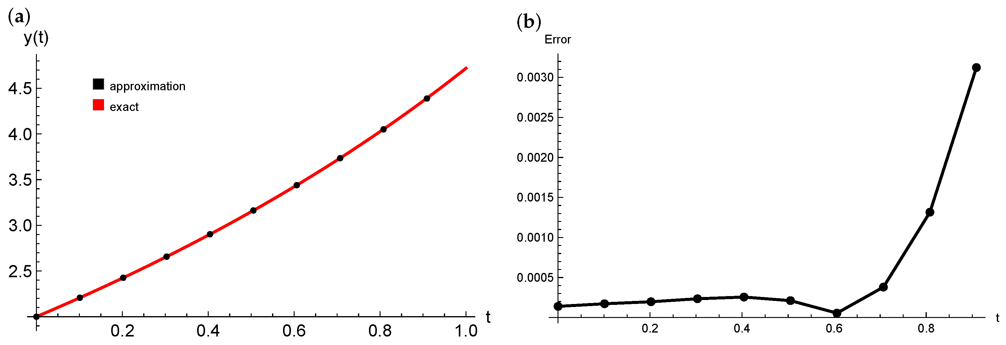
Now we show the comparison between results of Equation (5) solved through the standard variational iteration method in [42] and through PINNs. Solving Volterra integro-differential equations by PINNs, the integral term is approximated via numerical quadrature. Gaussian quadrature with a prescribed degree to approximate the integral was used. In Figure 18a the plot shows excellent agreement between the approximate solutions and the exact analytical solution (in case of PINNs) over the interval $t\in [0,1]$. Figure 18b illustrates the absolute error between the approximate and exact solutions, showing that the error remains minimal throughout the domain, with a slight increase near the upper boundary.

The results are obtained using 50 training points and three layers of neurons, each with eight neurons, while the activation function is tanh.

In

Table 13. Comparison of approximate and exact solutions.

t	Solutions [42]	PINNs	Exact Solution
0.0	2.00000	2.00014	2.00000
0.1	2.20517	2.20747	2.20730
0.2	2.42140	2.42609	2.42589
0.3	2.64986	2.65722	2.65699
0.4	2.89182	2.90216	2.90190
0.5	3.14867	3.16233	3.16212
0.6	3.42200	3.43931	3.43925
0.7	3.71440	3.73473	3.73511
0.8	4.03267	4.05036	4.05168
0.9	4.39798	4.38803	4.39115
1.0	4.87221	4.71233	4.71828

, we provide numerical values of the solution at selected time points. It compares the results from the variational iteration method [42], PINNs, and the exact solution. It can be seen that at $t=0.0$ both solutions perfectly match the exact solution. The solutions [42] are generally better than PINNs for $t\le 0.5$ while for larger t values PINNs unexpectedly outperform solutions [42].

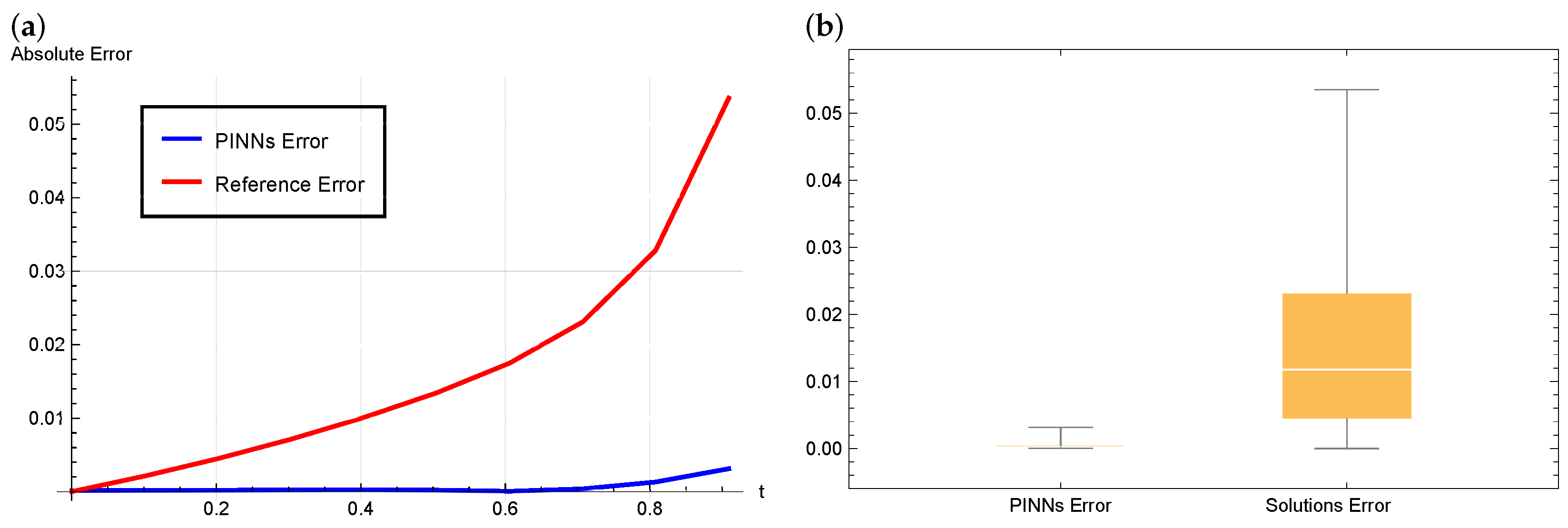
Comparing in terms of error metrics we can see that in

Table 14. Error metrics comparison between PINNs and solutions [42].

Metric	PINNs Error	Solutions [42] Error
Mean	0.000609	0.016428
Median	0.000223	0.011769
Standard Deviation	0.000953	0.016485
Mean Absolute Error	0.000609	0.016428
Root Mean Square Error	0.001090	0.022682

the mean and median errors for PINNs are an order of magnitude smaller than the reference solutions [42]. For example, PINNs’ mean error $0.000609$ is ∼27 times smaller than the reference error, i.e, $0.016428$. The standard deviation for PINNs is much lower, which testifies that it has more consistent performance as compared to the reference solutions [42].

In Figure 19, we give a comparative analysis of the absolute errors between the PINNs and the reference solutions [42]. In Figure 19a, the line plot shows that the PINNs approach consistently maintains a significantly lower error across the entire time interval compared to solutions [42]. The error for the reference method [42] grows steadily with time and reaches above $0.05$ near $t=0.9$, whereas the error for the PINNs solution remains very close to zero.

In Figure 19b, the boxplot provides a statistical summary of the error distributions. The median error and interquartile range for the PINNs is lower than those of reference solutions [42]. Moreover, the PINNs error exhibits minimal spread and lower maximum error.

These comparisons clearly demonstrate that the PINNs-based approach outperforms the traditional method in both average accuracy and robustness, making it a more reliable choice for solving these kind of Volterra integro-differential equations.

4. Conclusions

This work investigated the application of physics-informed neural networks (PINNs) to solve the Poisson equation, Burgers’ equation, and a fourth-order Volterra integro-differential equation. Comparative analysis with traditional numerical methods such as finite difference schemes and variational iteration techniques highlighted the flexibility and accuracy of PINNs, especially in scenarios where classical approaches encounter limitations. A systematic study of key hyperparameters—including the distribution of collocation points, network architecture, and activation functions—revealed their significant influence on both training efficiency and solution accuracy. Theoretical results further demonstrated that, for second-order linear elliptic and parabolic PDEs, PINN solutions converge strongly to the exact solution in the $C^0$ norm, and in the $H^1$ norm when boundary or initial conditions are enforced at all collocation points.

While the findings support the potential of PINNs as a viable alternative to conventional numerical solvers, challenges such as sensitivity to hyperparameter choices and high computational cost persist. All experiments were conducted using the DeepXDE library [43], which proved to be a reliable platform for model implementation and evaluation. Future work may focus on improving training strategies, automating hyperparameter tuning, and extending the framework to more complex or high-dimensional PDEs and inverse problems.

References

1. Raissi, M.; Perdikaris, P.; Karniadakis, G.E. Physics-informed neural networks: A deep learning framework for solving forward and inverse problems involving nonlinear partial differential equations. J. Comput. Phys. 2019, 378, 686–707. [Google Scholar] [CrossRef]
2. Raissi, M.; Perdikaris, P.; Karniadakis, G.E. Physics Informed Deep Learning (Part I): Data-driven Solutions of Nonlinear Partial Differential Equations. arXiv 2017, arXiv:1711.10561. [Google Scholar] [CrossRef]
3. Raissi, M.; Perdikaris, P.; Karniadakis, G.E. Physics Informed Deep Learning (Part II): Data-driven Discovery of Nonlinear Partial Differential Equations. arXiv 2017, arXiv:1711.10566. [Google Scholar] [CrossRef]
4. Cuomo, S.; Di Cola, V.S.; Giampaolo, F.; Rozza, G.; Raissi, M.; Piccialli, F. Scientific machine learning through physics–informed neural networks: Where we are and what’s next. J. Sci. Comput. 2022, 92, 88. [Google Scholar]
5. Brociek, R.; Pleszczyński, M. Differential Transform Method and Neural Network for Solving Variational Calculus Problems. Mathematics 2024, 12, 2182. [Google Scholar] [CrossRef]
6. Faroughi, S.A.; Pawar, N.M.; Fernandes, C.; Raissi, M.; Das, S.; Kalantari, N.K.; Kourosh Mahjour, S. Physics-Guided, Physics-Informed, and Physics-Encoded Neural Networks and Operators in Scientific Computing: Fluid and Solid Mechanics. J. Comput. Inf. Sci. Eng. 2024, 24, 040802. [Google Scholar] [CrossRef]
7. Usama, M.; Ma, R.; Hart, J.; Wojcik, M. Physics-Informed Neural Networks (PINNs)-Based Traffic State Estimation: An Application to Traffic Network. Algorithms 2022, 15, 447. [Google Scholar] [CrossRef]
8. Wang, S.; Wang, H.; Perdikaris, P. On the eigenvector bias of Fourier feature networks: From regression to solving multi-scale PDEs with physics-informed neural networks. Comput. Methods Appl. Mech. Eng. 2021, 384, 113938. [Google Scholar] [CrossRef]
9. Yuan, L.; Ni, Y.Q.; Deng, X.Y.; Hao, S. A-PINN: Auxiliary physics informed neural networks for forward and inverse problems of nonlinear integro-differential equations. J. Comput. Phys. 2022, 462, 111260. [Google Scholar] [CrossRef]
10. Xiang, Z.; Peng, W.; Liu, X.; Yao, W. Self-adaptive loss balanced Physics-informed neural networks. Neurocomputing 2022, 496, 11–34. [Google Scholar] [CrossRef]
11. Dwivedi, V.; Parashar, N.; Srinivasan, B. Distributed learning machines for solving forward and inverse problems in partial differential equations. Neurocomputing 2021, 420, 299–316. [Google Scholar] [CrossRef]
12. Lee, J. Anti-derivatives approximator for enhancing physics-informed neural networks. Comput. Methods Appl. Mech. Eng. 2024, 426, 117000. [Google Scholar] [CrossRef]
13. McClenny, L.D.; Braga-Neto, U.M. Self-adaptive physics-informed neural networks. J. Comput. Phys. 2023, 474, 111722. [Google Scholar] [CrossRef]
14. Brociek, R.; Pleszczyński, M. Differential Transform Method (DTM) and Physics-Informed Neural Networks (PINNs) in Solving Integral–Algebraic Equation Systems. Symmetry 2024, 16, 1619. [Google Scholar] [CrossRef]
15. Ren, Z.; Zhou, S.; Liu, D.; Liu, Q. Physics-Informed Neural Networks: A Review of Methodological Evolution, Theoretical Foundations, and Interdisciplinary Frontiers Toward Next-Generation Scientific Computing. Appl. Sci. 2025, 15, 92. [Google Scholar] [CrossRef]
16. Lawal, Z.K.; Yassin, H.; Lai, D.T.C.; Che Idris, A. Physics-Informed Neural Network (PINN) Evolution and Beyond: A Systematic Literature Review and Bibliometric Analysis. Big Data Cogn. Comput. 2022, 6, 140. [Google Scholar] [CrossRef]
17. Coutinho, E.J.R.; Dall’Aqua, M.; McClenny, L.; Zhong, M.; Braga-Neto, U.; Gildin, E. Physics-informed neural networks with adaptive localized artificial viscosity. J. Comput. Phys. 2023, 489, 112265. [Google Scholar] [CrossRef]
18. Diao, Y.; Yang, J.; Zhang, Y.; Zhang, D.; Du, Y. Solving multi-material problems in solid mechanics using physics-informed neural networks based on domain decomposition technology. Comput. Methods Appl. Mech. Eng. 2023, 413, 116120. [Google Scholar] [CrossRef]
19. Lazovskaya, T.; Malykhina, G.; Tarkhov, D. Physics-Based Neural Network Methods for Solving Parameterized Singular Perturbation Problem. Computation 2021, 9, 97. [Google Scholar] [CrossRef]
20. Jagtap, A.D.; Mao, Z.; Adams, N.; Karniadakis, G.E. Physics-informed neural networks for inverse problems in supersonic flows. J. Comput. Phys. 2022, 466, 111402. [Google Scholar] [CrossRef]
21. Hornik, K.; Stinchcombe, M.; White, H. Multilayer feedforward networks are universal approximators. Neural Netw. 1989, 2, 359–366. [Google Scholar] [CrossRef]
22. Baydin, A.G.; Pearlmutter, B.A.; Radul, A.A.; Siskind, J.M. Automatic differentiation in machine learning: A survey. J. Mach. Learn. Res. 2018, 18, 1–43. [Google Scholar]
23. Uddin, Z.; Ganga, S.; Asthana, R.; Ibrahim, W. Wavelets based physics informed neural networks to solve non-linear differential equations. Sci. Rep. 2023, 13, 2882. [Google Scholar] [CrossRef] [PubMed]
24. Shin, Y.; Darbon, J.; Karniadakis, G.E. On the convergence of physics informed neural networks for linear second-order elliptic and parabolic type PDEs. arXiv 2020, arXiv:2004.01806. [Google Scholar] [CrossRef]
25. Doumèche, N.; Biau, G.; Boyer, C. Convergence and error analysis of PINNs. arXiv 2023, arXiv:2305.01240. [Google Scholar] [CrossRef]
26. Yoo, J.; Lee, H. Robust error estimates of PINN in one-dimensional boundary value problems for linear elliptic equations. arXiv 2024, arXiv:2407.14051. [Google Scholar] [CrossRef]
27. De Ryck, T.; Mishra, S. Error analysis for physics-informed neural networks (PINNs) approximating Kolmogorov PDEs. Adv. Comput. Math. 2022, 48, 79. [Google Scholar] [CrossRef]
28. Kingma, D.P. Adam: A method for stochastic optimization. arXiv 2014, arXiv:1412.6980. [Google Scholar]
29. Holm, D.D. Applications of Poisson geometry to physical problems. Geom. Topol. Monogr. 2011, 17, 221–384. [Google Scholar]
30. Nolasco, C.; Jácome, N.; Hurtado-Lugo, N. Applications of the Poisson and diffusion equations to materials science. J. Phys. Conf. Ser. 2020, 1587, 012014. [Google Scholar]
31. Klopfenstein, R.; Wu, C. Computer solution of one-dimensional Poisson’s equation. IEEE Trans. Electron Devices 1975, 22, 329–333. [Google Scholar] [CrossRef]
32. Bhardwaj, S.; Gohel, H.; Namuduri, S. A Multiple-Input Deep Neural Network Architecture for Solution of One-Dimensional Poisson Equation. IEEE Antennas Wirel. Propag. Lett. 2019, 18, 2244–2248. [Google Scholar] [CrossRef]
33. Kraichnan, R.H. Lagrangian-history statistical theory for Burgers’ equation. Phys. Fluids 1968, 11, 265–277. [Google Scholar] [CrossRef]
34. Xie, S.S.; Heo, S.; Kim, S.; Woo, G.; Yi, S. Numerical solution of one-dimensional Burgers’ equation using reproducing kernel function. J. Comput. Appl. Math. 2008, 214, 417–434. [Google Scholar] [CrossRef]
35. Inan, B.; Bahadir, A.R. Numerical solution of the one-dimensional Burgers’ equation: Implicit and fully implicit exponential finite difference methods. Pramana 2013, 81, 547–556. [Google Scholar] [CrossRef]
36. Bonkile, M.P.; Awasthi, A.; Lakshmi, C.; Mukundan, V.; Aswin, V. A systematic literature review of Burgers’ equation with recent advances. Pramana 2018, 90, 69. [Google Scholar] [CrossRef]
37. Kutluay, S.; Bahadir, A.; Özdeş, A. Numerical solution of one-dimensional Burgers equation: Explicit and exact-explicit finite difference methods. J. Comput. Appl. Math. 1999, 103, 251–261. [Google Scholar] [CrossRef]
38. Mukundan, V.; Awasthi, A. Efficient numerical techniques for Burgers’ equation. Appl. Math. Comput. 2015, 262, 282–297. [Google Scholar] [CrossRef]
39. Brunner, H. Collocation Methods for Volterra Integral and Related Functional Differential Equations; Cambridge University Press: Cambridge, UK, 2004; Volume 15. [Google Scholar]
40. Volterra, V. Leçons sur la Théorie Mathématique de la Lutte pour la Vie; Gauthier Villars: Paris, France, 1931. [Google Scholar]
41. Joseph, D.D.; Preziosi, L. Heat waves. Rev. Mod. Phys. 1989, 61, 41. [Google Scholar] [CrossRef]
42. Otaide, I.J.; Oluwayemi, M.O. Numerical treatment of linear volterra integro differential equations using variational iteration algorithm with collocation. Partial. Differ. Equ. Appl. Math. 2024, 10, 100693. [Google Scholar] [CrossRef]
43. Lu, L.; Meng, X.; Mao, Z.; Karniadakis, G.E. DeepXDE: A deep learning library for solving differential equations. SIAM Rev. 2021, 63, 208–228. [Google Scholar] [CrossRef]
Figure 1. Schematic diagram of a physics-informed neural network.
Symmetry 17 01698 g001
Figure 2. Plots of the approximated and exact solution (a) and the absolute approximation error (b).
Symmetry 17 01698 g002
Figure 3. Train and test loss during solution of (2).
Symmetry 17 01698 g003
Figure 4. Mean error as a function of the number of network parameters (Poisson equation).
Symmetry 17 01698 g004
Figure 5. Training time as a function of the number of network parameters (Poisson equation).
Symmetry 17 01698 g005
Figure 6. Error distribution obtained from the PINN for selected hyperparameters concerning the number of hidden layers and neurons (Poisson equation).
Symmetry 17 01698 g006aSymmetry 17 01698 g006b
Figure 7. Prediction from PINN for 2 hidden layers and 20 neurons (Poisson equation).
Symmetry 17 01698 g007
Figure 8. Plots of the approximated and exact solution (a) and the absolute approximation error (b).
Symmetry 17 01698 g008
Figure 9. Train and test loss.
Symmetry 17 01698 g009
Figure 10. Comparison of solutions for different values of t and x = 0.5 .
Symmetry 17 01698 g010
Figure 11. Comparison of absolute errors of the BDF-1 method for different values of N with the PINN method as a function of the spatial coordinate x at t = 0.5 .
Symmetry 17 01698 g011
Figure 12. Mean error as a function of the number of network parameters (Burgers’ equation).
Symmetry 17 01698 g012
Figure 13. Training time as a function of the number of network parameters (Burgers’ equation).
Symmetry 17 01698 g013
Figure 14. Prediction from PINN for 6 hidden layers and 30 neurons (Burgers’ equation).
Symmetry 17 01698 g014
Figure 15. Error distribution obtained from the PINN for selected hyperparameters concerning the number of hidden layers and neurons (Burgers’ equation).
Symmetry 17 01698 g015
Figure 16. Error distribution obtained from the PINN for selected hyperparameters concerning the number of hidden layers and neurons (Volterra equation).
Symmetry 17 01698 g016
Figure 17. Prediction from PINN for 6 hidden layers and 50 neurons (VIDE).
Symmetry 17 01698 g017
Figure 18. Plots of the approximated and exact solution (a) and the absolute approximation error (b).
Symmetry 17 01698 g018
Figure 19. Illustration of comparative analysis of the absolute errors, (a) absolute error for the reference solution and that obtained with PINN; (b) boxplot of the statistical summary of the error distributions.
Symmetry 17 01698 g019