Article

On a Novel Iterative Algorithm in CAT(0) Spaces with Qualitative Analysis and Applications

1
Abdus Salam School of Mathematical Sciences, Government College University, Lahore 54000, Pakistan
2
Department of Mechanical Engineering Science, Faculty of Engineering and the Built Environment, University of Johannesburg, Johannesburg 2006, South Africa
3
Department of Medical Research, China Medical University, Taichung 406040, Taiwan
4
Department of Mathematics and Informatics, National University of Science and Technology Politehnica Bucharest, 060042 Bucharest, Romania
*
Author to whom correspondence should be addressed.
Symmetry 2025, 17(10), 1695; https://doi.org/10.3390/sym17101695
Submission received: 2 September 2025 / Revised: 3 October 2025 / Accepted: 7 October 2025 / Published: 9 October 2025

Abstract

This study presents a novel and efficient iterative scheme in the setting of CAT(0) spaces and investigates the convergence properties for a generalized class of mappings satisfying the Garcia–Falset property using the proposed iterative scheme. Strong and weak convergence results are established in CAT(0) spaces, generalizing many existing results in the literature. Furthermore, we discuss the stability and data dependence of the new iterative process. Numerical experiments include an analysis of error values, the number of iterations, and computational time, providing a comprehensive assessment of the method’s performance. Moreover, graphical comparisons demonstrate the efficiency and reliability of the approach. The obtained results are utilized in solving integral equations. Additionally, the paper concludes with a polynomiographic study of the newly introduced iterative process, in comparison with standard algorithms, such as Newton, Halley, or Kalantari’s B 4 iteration, emphasizing symmetry properties.
MSC:
47H09; 47H10; 54H25

1. Preliminaries and Introduction

Throughout this paper, F ( T ) denotes the set of fixed points associated with an operator T on an underlying space. Let us recall the basic definitions and known results.
Let ( X , d ) be a metric space. A geodesic path joining x X to y X is a mapping γ : [ 0 , l ] X , such that γ ( 0 ) = x , γ ( l ) = y and d γ ( t ) , γ ( t ) = t t , for all t , t [ 0 , l ] , where d ( x , y ) = l . The image of γ denoted by [ x , y ] is called a geodesic segment joining x and y. The space X is called geodesic space if every two points of X are joined by a geodesic and X is said to be uniquely geodesic if there is exactly one geodesic joining x and y for each x , y X . A subset Y X is said to be convex if Y contains every geodesic segment joining any two of its points.
A geodesic triangle Δ x 1 , x 2 , x 3 consists of three points x 1 , x 2 , x 3 in X called the vertices of Δ , and a geodesic segment between each pair of vertices called the edges of Δ . A comparison triangle for a geodesic triangle Δ x 1 , x 2 , x 3 in X is a triangle Δ ¯ x ¯ 1 , x ¯ 2 , x ¯ 3 in the Euclidean plane E 2 such that d E 2 x ¯ i , x ¯ j = d x i , x j , for i , j { 1 , 2 , 3 } . A geodesic space is called a C A T ( 0 ) space if all geodesic triangles satisfy the following comparison axiom.
Let Δ ¯ be a comparison triangle for a geodesic triangle Δ in X; then, Δ is said to satisfy the comparison axiom if for all x , y Δ and all comparison points x ¯ , y ¯ Δ ¯ , we have
d ( x , y ) d E 2 ( x ¯ , y ¯ ) .
The above inequality is known as C A T ( 0 ) inequality.
If x , y 1 , y 2 are points in a geodesic space and if y 0 is the midpoint of the segment y 1 , y 2 , that is d ( y 1 , y 0 ) = d ( y 0 , y 2 ) = 1 2 d ( y 1 , y 2 ) , then the following inequality
d 2 x , y 0 1 2 d 2 x , y 1 + 1 2 d 2 x , y 2 1 4 d 2 y 1 , y 2
is known as a midpoint inequality. A geodesic space is a C A T ( 0 ) space if and only if it satisfies the midpoint inequality [1].
Let { x n } be a bounded sequence in a C A T ( 0 ) space X. For x X , we define
r x , x n = lim sup n d x , x n .
The asymptotic radius of a given sequence { x n } , denoted by r { x n } , is given by
r { x n } = inf { r x , { x n } : x X } .
The asymptotic center of { x n } denoted by A { x n } is given by
A { x n } = { x X : r x , { x n } = r { x n } } .
In CAT(0) spaces, the asymptotic center is unique, which enables us to study the Δ –convergence, the analogue of the notion of weak convergence in Banach spaces.
Definition 1
([2]). A sequence { x n } in a C A T ( 0 ) space X is called Δ–convergent to x X . If for any subsequence { x n k } of { x n } , the point x is the unique asymptotic center of { x n k } , we write Δ lim n x n = x and call x the Δ–limit of { x n } .
It is known that every C A T ( 0 ) space has an Opial’s property for any given sequence { x n } in a C A T ( 0 ) space, such that { x n } is Δ –convergent to x. Then for any y X with x y , we have
lim sup n d ( x n , x ) < lim sup n d ( x n , y ) .
We now collect some elementary facts about C A T ( 0 ) spaces, which are needed in the sequel.
Lemma 1
([2]). Let ( X , d ) be a C A T ( 0 ) space.
1. 
Every bounded sequence in X always possesses a Δ–convergent subsequence.
2. 
If { x n } is a bounded sequence in a closed convex subset K of X, the asymptotic center of { x n } lies in K.
3. 
If { x n } is a bounded sequence with A ( { x n } ) = x and { x n k } is the subsequence of { x n } with A ( { x n k } ) = y , and { d ( x n , y ) } converges, then x = y .
Lemma 2
([2]). Let ( X , d ) be a C A T ( 0 ) space.
1. 
For any x , y X and t [ 0 , 1 ] , there is a unique point z [ x , y ] , such that
d ( x , z ) = t d ( x , y )
and
d ( y , z ) = ( 1 t ) d ( x , y ) ,
where the unique point z given above is denoted by ( 1 t ) x t y .
2. 
For any x , y , z X and t [ 0 , 1 ] , we have
d ( ( 1 t ) x t y , z ) ( 1 t ) d ( x , z ) + t d ( y , z ) .
In the framework of CAT(0) spaces, the symbol ⊕ is commonly used to denote the geodesic convex combination of two points. In other words, this symbol serves as the analogue of linear interpolation in Euclidean spaces, but adapted to the curved geometry of CAT(0) spaces, where geodesics replace straight lines.
Lemma 3
([3]). Let { α n } be a sequence in [ a , b ] , where a , b ( 0 , 1 ) . If the sequences { x n } , { y n } in the C A T ( 0 ) space satisfy lim sup n d ( x n , x ) r , lim sup n d ( y n , x ) r and
lim sup n d ( ( 1 α n ) x n α n y n , x ) r ,
for some r 0 , then we have
lim n d ( x n , y n ) = 0 .
Definition 2
([4]). A self-mapping T defined on a nonempty subset K of C A T ( 0 ) space X is said to satisfy condition ( I ) if there is a nondecreasing function g : [ 0 , ) [ 0 , ) with g ( 0 ) = 0 and g ( c ) > 0 , for all c > 0 , such that for any x K , we have
d ( x , T x ) g inf { d ( x , y ) : y F ( T ) } .
Let us recall that, a mapping T defined on a subset K of CAT(0) space is called Banach contraction if there exists a κ [ 0 , 1 ) , such that
d ( T x , T y ) κ d ( x , y ) ,
for all x , y K .
If we set κ = 1 in the above definition, then a mapping T is said to be nonexpansive. In 2008, Suzuki [5] introduced a more general class of mappings by relaxing the nonexpansive condition, and established both existence and convergence results for such mappings in the framework of Banach spaces.
Definition 3.
A self-mapping T defined on a nonempty subset K of C A T ( 0 ) space X is said to satisfy condition ( C ) if, for any x , y K , we have
1 2 d ( x , T x ) d ( x , y ) implies d ( T x , T y ) d ( x , y ) .
The mapping satisfying condition ( C ) is also called Suzuki generalized nonexpansive mapping. In [5], it was shown that a mapping satisfying condition ( C ) has the following property:
d ( x , T y ) 3 d ( x , T x ) + d ( x , y ) ,
for all x , y K .
In the case of nonexpansive mapping T, it is obvious to note that
d ( x , T y ) d ( x , T x ) + d ( x , y ) ,
for all x , y K .
Motivated by these fact, Garcia et al. [6] introduced a general class of mappings and obtained some fixed point results called the class of mapping with condition ( E ) .
Definition 4.
A mapping T defined on a nonempty subset K of C A T ( 0 ) space X is said to satisfy the Garcia–Falset property if there is μ 1 , such that
d ( x , T y ) μ d ( x , T x ) + d ( x , y ) ,
for all x , y K .
Thus, every nonexpansive mapping satisfies the Garcia–Falset property for μ = 1 , and a mapping with condition ( C ) also satisfies the Garcia–Falset property for μ = 3 .
Lemma 4.
Let T be a mapping satisfying the Garcia–Falset property defined on a nonempty subset K of C A T ( 0 ) space X. Then, F ( T ) is closed.
Lemma 5.
Let T be a mapping satisfying the Garcia–Falset property defined on nonempty subset K of C A T ( 0 ) space X. If F ( T ) , then T is quasi-nonexpansive. More precisely,
d ( x , T y ) d ( x , y ) ,
for all y K and x F ( T ) .
The theory of nonexpansive mappings forms a crucial part of nonlinear analysis, with a wide range of applications. It all started in 1965 when three mathematicians, Browder [7], Gohde [8], and Kirk [9], independently investigated important fixed point results for the class of nonexpansive mappings. Later, many researchers developed new classes of mappings to extend the existing results on nonexpansive mappings. In 1973, Kannan [10] introduced a class of mappings called Kannan mappings, which need not be continuous and are independent of the Banach contraction principle. In 1980, combining the notions of nonexpansive and Kannan mappings, Gregus [11] introduced the Reich nonexpansive mappings. Later, α -nonexpansive mappings, an extended class of generalized nonexpansive mappings, were introduced by Aoyama et al. [12], leading to several interesting fixed point results in this direction. In 2017, Pant and Shukla [13] considered a class of nonexpansive-type mappings known as generalized α -nonexpansive mappings. Recently, Pandey et al. [14] presented a significant extension of nonexpansive mappings, known as generalized α -Reich–Suzuki nonexpansive mappings, and showed that this class satisfies the Garcia–Falset property for μ = 3 + α 1 α . It is shown in [14] that this class of mappings is more general than Suzuki generalized nonexpansive mappings, and all the mappings discussed above fall into the class of generalized α -Reich–Suzuki nonexpansive mappings. Consequently, all these mappings belong to the class of mappings satisfying the Garcia–Falset property.
Similarly, Karapinar [15] introduced several classes of operators satisfying certain contractive conditions that generalize existing mappings with condition ( C ) , namely Reich–Suzuki–(C) (denoted RSC), Reich–Chatterjee–Suzuki– ( C ) (denoted RCSC), and Hardy–Rogers–Suzuki– ( C ) (denoted HRSC), which also satisfy the Garcia–Falset property with μ = 7 , μ = 9 , and μ = 15 , respectively. Moreover, the class of operators defined by Bejenaru and Postolache [16] satisfies the Garcia–Falset property with μ = 3 . In this way, many well-known nonexpansive-type mappings ultimately satisfy the Garcia–Falset property.
In nonlinear analysis, approximating the solutions of nonlinear operator equations and inclusions poses a significant research challenge, particularly when solving fixed point equations for which an analytic solution cannot be obtained. The Banach contraction principle not only guarantees the existence and uniqueness of solutions for fixed point equations involving contraction operators, but also provides one of the simplest constructive methods, known as the Picard iteration process, to approximate the solution [17]. Given an arbitrary initial guess x 0 in a closed subset K of a complete metric space X, a sequence x n can be constructed as follows:
x n + 1 = T x n ,
for all n N .
If the contraction operator T in the above processes is replaced with a nonexpansive mapping, the resulting sequence may fail to converge to the fixed point of T even if the fixed point is known.
To address this, various iterative procedures have been developed to approximate the fixed points of nonexpansive mappings and their different invariants. The foundational algorithm for nonexpansive mappings include one-step Mann iteration [18] given as follows. Let x 0 be an arbitrary point in a closed and convex subset K of a normed space X. Define a sequence { x n } in X by
x n + 1 = ( 1 α n ) x n + α n T x n ,
for all n N , where { α n } is a real sequence in [ 0 , 1 ] . The Mann iterative algorithm has certain limitations: it fails when a nonexpansive mapping is replaced by a pseudocontractive Lipschitzian mapping, highlighting the need for a modified iterative approach. To address this limitation, Ishikawa [19] defined a two-step iteration scheme as follows. Let x 0 be an arbitrary point in a closed and convex subset K of a normed space X. Define a sequence { x n } in X by
y n = ( 1 α n ) x n + α n T x n x n + 1 = ( 1 β n ) y n + β n T y n ,
for all n N , where { α n } and { β n } are real sequences in [ 0 , 1 ] .
Noor [20] introduced a three-step iterative process to improve the convergence behavior of the Ishikawa iterative scheme. Let x 0 be an arbitrary point in a closed and convex subset K of a normed space X. Define a three-step sequence { x n } in X by
z n = ( 1 α n ) x n + α n T x n y n = ( 1 β n ) x n + β n T z n x n + 1 = ( 1 γ n ) x n + γ n T y n ,
for all n N , where { α n } , { β n } and { γ n } are real sequences in [ 0 , 1 ] .
The focus of improving the convergence rate of fixed point iterative algorithms opened new avenues of developing iterative schemes, even in the cases where existing algorithms are already applicable to the given class of operators. In this direction, Abbas and Nazir [21] defined the iteration scheme
z n = ( 1 α n ) x n + α n T x n y n = ( 1 β n ) T x n + β n T z n x n + 1 = ( 1 γ n ) T z n + γ n T y n ,
for all n N , where { α n } , { β n } , and { γ n } are real sequences in [ 0 , 1 ] and x 0 is an arbitrary point in a convex subset K of a normed space X.
Sintunavarat and Pitea [22] introduced the S n iteration to approximate the fixed points of Berinde-type operators as follows:
z n = ( 1 α n ) x n + α n T x n y n = ( 1 β n ) x n + β n z n x n + 1 = ( 1 γ n ) T y n + γ n T z n ,
for all n N , where { α n } , { β n } , and { γ n } are real sequences in [ 0 , 1 ] and x 0 is an arbitrary point in a convex subset K of a normed space X.
Recently, Aftab et al. [23] developed a D * iterative procedure, given by
z n = T ( 1 α n ) x n + α n T x n y n = T ( 1 β n ) z n + β n T z n x n + 1 = T ( 1 γ n ) y n + γ n T y n ,
for all n N , where { α n } , { β n } , and { γ n } are real sequences in [ 0 , 1 ] and x 0 is an arbitrary point in a convex subset K of a normed space X.
Lamba and Panwar et al. [24] introduced Picard S * iterative algorithms, a four-step iterative scheme for approximating the fixed points of generalized nonexpansive mappings, as follows:
w n = ( 1 α n ) x n + α n T x n z n = ( 1 β n ) T x n + β n T w n y n = ( 1 γ n ) T x n + γ n T z n x n + 1 = T y n ,
for all n N , where { α n } , { β n } , and { γ n } are real sequences in [ 0 , 1 ] and x 0 is an arbitrary point in a convex subset K of a normed space X.
Recently, Jia et al. [25] proposed the Picard–Thakur hybrid iterative scheme, which is given as
w n = ( 1 α n ) x n + α n T x n z n = ( 1 β n ) w n + β n T w n y n = ( 1 γ n ) T w n + γ n T z n x n + 1 = T y n ,
for all n N , where { α n } , { β n } , and { γ n } are real sequences in [ 0 , 1 ] and x 0 is an arbitrary point in a convex subset K of a normed space X.
As mentioned earlier, CAT(0) spaces provide a flexible framework for studying geometric and topological properties, such as the convexity of sets and functions, and the convergence of sequences in a purely metric setting, without relying on vector operations. They broaden the scope of analysis beyond linear structures while retaining powerful geometric and analytic properties.
Motivated by these findings, we develop a novel iterative technique in the framework of CAT(0) spaces, designed to refine and generalize existing algorithms. Let T be a mapping defined on a nonempty subset K of a CAT(0) space, and let x 0 K be an arbitrary point. Define a sequence { x n } by
w n = T ( 1 α n ) x n α n T x n z n = T ( 1 β n ) w n β n T w n y n = T ( 1 γ n ) z n γ n T z n x n + 1 = T y n ,
for all n N , where { α n } , { β n } , and { γ n } are real sequences in [ 0 , 1 ] . The iteration scheme exhibits different characteristics based on the parameter values involved therein.
When all the parameters are set to zero or one, the iteration scheme reduces to repeated applications of the Picard iteration operator. With arbitrary parameter values, however, the scheme transforms into a novel formulation, distinct from existing methods in the current literature.
In this paper, we study strong and Δ –convergence results for a generalized class of mappings using the proposed iterative process. A comparative analysis with existing iterative methods demonstrates that the proposed method is more efficient and exhibits faster convergence for generalized contraction mappings. A stability theorem further guarantees the reliability of the new method. Moreover, our results are new even in the framework of Banach spaces, thereby generalizing several well-known convergence results in Banach spaces.

2. Approximation Results

In this section, we present several weak and strong convergence results for a new proposed iterative scheme (1) for the mappings satisfying Garcia–Falset property ( E ) in the framework of CAT(0) spaces. Throughout the section, we assume that a mapping T is defined on a nonempty closed convex subset K of CAT(0) space X and satisfies the Definition 4. Let the sequence x n be defined by (1).
Theorem 1.
If F ( T ) , then the lim n d x n , g exists, for all g F ( T ) .
Proof. 
Let g F ( T ) . We get
d w n , g = d T 1 α n x n α n T x n , g d 1 α n x n α n T x n , g 1 α n d x n , g + α n d T x n , g 1 α n d x n , g + α n d x n , g d x n , g .
On the other hand,
d z n , g = d T 1 β n w n β n T w n , g d 1 β n w n β n T w n , g 1 β n d w n , g + β n d T w n , g 1 β n d w n , g + β n d w n , g d w n , g .
Using similar arguments, we obtain
d y n , g = d T 1 γ n z n γ n T z n , g d 1 γ n z n γ n T z n , g 1 γ n d z n , g + γ n d T z n , g 1 γ n d z n , g + γ n d z n , g d z n , g .
Finally,
d x n + 1 , g = d T y n , g d y n , g d z n , g d w n , g d x n , g .
This shows that the sequence d x n , g is both bounded and non-increasing. Thus, the limit of the sequence lim n d x n , g exists. □
The following theorem provides the necessary and sufficient condition for the existence of a fixed point of a mapping T.
Theorem 2.
We have that F ( T ) if and only if the sequence x n is bounded and lim n d T x n , x n = 0 .
Proof. 
Suppose that lim n d x n , T x n = 0 and the sequence x n is bounded. We will show F ( T ) . For any g A x n , we have
r T g , x n = lim sup n d x n , T g lim sup n μ d T x n , x n + d x n , g = μ lim sup n d T x n , x n + lim sup n d x n , g = lim sup n d x n , g = r g , x n .
This implies that T g A { x n } . Since A { x n } consists of a single element. This follows that g F ( T ) .
Conversely, suppose that g F ( T ) . We show lim n d x n , T x n = 0 . By Theorem 1, x n is bounded and lim n d x n , g exists. Consider
ξ = lim n d x n , g .
Using Lemma 5, we have
d T x n , g d x n , g .
This implies
lim sup n d T x n , g lim sup n d x n , g = ξ .
From the proof of Theorem 1, we obtain
d w n , g d x n , g .
This gives
lim sup n d w n , g lim sup n d x n , g = ξ .
Again, from the proof of Theorem 1, we have
d x n + 1 , g d w n , g .
This implies
ξ = lim inf n d x n + 1 , g lim inf n d w n , g .
From (4) and (5), we obtain
ξ = lim n d w n , g .
Thus, we have
ξ = lim n d w n , g = lim n d T ( ( 1 α n ) x n α n T x n , g ) lim n d ( 1 α n ) x n α n T x n , g lim n ( 1 α n ) d ( x n , g ) + α n d ( T x n , g ) lim n ( 1 α n ) d ( x n , g ) + lim n d ( T x n , g ) ξ .
This leads to
lim n d ( 1 α n ) x n α n T x n , g = ξ .
From (2), (3), (6), and Lemma 3, we have
lim n d T x n , x n = 0 ,
which completes the proof. □
We now establish weak convergence result using Opial’s condition in CAT(0) space.
Theorem 3.
If F ( T ) , then x n is Δ–convergent to an element in F ( T ) .
Proof. 
Set ω ( x n ) = A ( { u n } ) , where union is taken over all subsequences of { x n } . If x ω ( x n ) , then there exists a subsequence { x n k } of { x n } such that A ( { x n k } ) = x .
By Theorem 2, { x n k } is bounded. Using Lemma 1 (i) and (ii), we have a subsequence { x n j } of { x n k } such that, for some y K ,
Δ lim j x n j = y .
It follows from Theorem 2 that y F ( T ) , and by Theorem 1, lim n d ( x n , y ) exists. Suppose that x y . Using Opial’s condition and uniqueness of asymptotic center, we get
lim sup n d x n , y = lim sup j d x n j , y < lim sup j d x n j , x lim sup k d x n k , x < lim sup k d x n k , y = lim sup n d x n , y ,
which is absurd. Therefore, x = y . To show that x is the asymptotic center of every subsequence of { x n } , let z ω ( x n ) since { x n k } is a subsequence of { x n } with A ( { x n k } ) = x , and lim n d ( x n , x ) exists. By Lemma 1 (iii), we have x = z . Therefore, { x n } is Δ –convergent to x F ( T ) . □
Now, we establish some strong convergence results using the underlying class of mappings in the setting of CAT(0) space.
Theorem 4.
If K is Δ–compact and F ( T ) , then { x n } strongly converges to an element in F ( T ) .
Proof. 
By Theorem 2, we have lim n d x n , T x n = 0 . Due to the compactness of K, we can find a subsequence x n j of x n , which is Δ –convergent to z K . Hence, we obtain
lim sup j d x n j , T z lim sup j μ d T x n j , x n j + d x n j , z .
On taking the limit as j , and the uniqueness of asymptotic center, we have T z = z . By Theorem 1, lim n d x n , z exists for any z F ( T ) . Therefore, x n converges strongly to z. □
Theorem 5.
If F ( T ) and lim inf n d x n , F ( T ) = 0 , then x n converges strongly to a fixed point of T.
Proof. 
Suppose { x n } converges strongly to g F ( T ) , then
lim inf n d ( x n , g ) = 0 .
It follows that
lim inf n d ( x n , F ( T ) ) = 0 .
Conversely, suppose that lim inf n d x n , F ( T ) = 0 . So, a subsequence { x n k } of { x n } and { x k } in F ( T ) exists such that
d x n k , x k < 1 2 k , for all k N .
On the other hand, we have
d x n k + 1 , x k d x n k , x k 1 2 k .
Now, using the triangle inequality
d x k + 1 , x k d x k + 1 , x n k + d x n k , x k 1 2 k + 1 2 k 1 2 k 1 0 , whenever k .
Hence, { x k } is a Cauchy sequence. Using Lemma 4, { x k } converges to g F ( T ) . Thus, we have
d ( x n k , g ) d ( x n k , x k ) + d ( x k , g ) .
This implies that { x n k } converges to g F ( T ) on taking limit as k . By Theorem 1, lim inf n d x n , g exists, for all g F ( T ) . Therefore, { x n } converges strongly to g F ( T ) . □
Theorem 6.
If F ( T ) and T satisfies condition ( I ) , then { x n } converges strongly to g F ( T ) .
Proof. 
By Theorem 1, lim n d ( x n , g ) exists for all g F ( T ) . So, lim n d ( x n , F ( T ) ) exists. Using Theorem 2, we have
lim n d ( x n , T x n ) = 0 .
Since T satisfies condition ( I ) , using the Definition 2, we get
d ( x n , T x n ) f d ( x n , F ( T ) ) .
It follows from (7) that
lim n f d ( x n , F ( T ) ) = 0 .
Since g is a nondecreasing function with f ( 0 ) = 0 and f ( c ) > 0 , for all c > 0 , from (8), we get
lim n ( d ( x n , F ( T ) ) ) = 0 .
By Theorem 5, the sequence { x n } converges strongly to g F ( T ) . □

3. Stability and Data Dependence

In general terms, an iterative scheme leading to a unique fixed point is regarded as stable if its convergence remains unaffected by the numerical inaccuracies that may arise at each step of the iteration. The concept of T-stability was originally put forward by Harder and Hicks [26], whose work represents a cornerstone in this field, providing definitions both in the setting of metric spaces and in that of normed spaces. It is also worth mentioning that the stability of iterative processes is an important point of interest (see [27], for instance, where it is studied for the Picard iteration).
Definition 5
([26]). Suppose that T is a given mapping and x n + 1 = f ( T , x n ) is an iterative process constructed with T and the past approximation x n , where f is a function which defines the iterative process, and the exact sequence { x n } converges to the fixed point g of a mapping T. An iterative sequence is called T-stable if for the perturbed sequence { y n } given by ϵ n = d ( y n + 1 , f ( T , y n ) ) , we have
lim n ϵ n = 0 if and only if lim n y n = g .
The following lemma will serve as a key tool in deriving the forthcoming results.
Lemma 6
([28]). Let { a n } and { c n } be non-negative real-number sequences satisfying
a n + 1 ( 1 b n ) a n + c n ,
with b n ( 0 , 1 ) , for all n N , n = 1 b n = and lim n c n b n = 0 . Then, lim n a n = 0 .
As a first step, the next theorem establishes the convergence of the new iterative process to a fixed point of T.
Theorem 7.
Let T be contraction mapping defined on a nonempty closed convex subset K of CAT(0) space X and { x n } an iteration scheme defined by (1). If n = 0 α n = or n = 0 β n = , then { x n } strongly converges to g F ( T ) .
Proof. 
First of all, we can say that
d w n , g = d T ( 1 α n ) x n α n T x n , g κ d ( 1 α n ) x n α n T x n , g κ { 1 α n d x n , g + α n d T x n , g } κ { 1 α n x n , g + α n κ x n , g } = κ { 1 α n ( 1 κ ) } d x n , g .
By proceeding in a similar way, we can assert that
d z n , g = d T ( 1 β n ) w n β n T w n , g κ d ( 1 β n ) w n β n T w n , g κ 1 β n d w n , g + β n d T w n , g κ 1 β n w n , g + β n κ w n , g = κ d w n , g κ 2 { 1 α n ( 1 κ ) } d x n , g .
Finally, we may state that
d y n , g = d T ( 1 γ n ) z n γ n T z n , g κ d ( 1 γ n ) z n γ n T z n , g κ 1 γ n d z n , g + γ n d T z n , g κ 1 γ n z n , g + γ n κ z n , g = κ d z n , g κ 3 { 1 α n ( 1 κ ) } d x n , g
and
d x n + 1 , g = d T y n , g κ d y n , g κ 4 1 α n ( 1 κ ) d x n , g .
Using the fact that 1 α n ( 1 κ ) < 1 and κ ( 0 , 1 ) , we obtain that
d x n + 1 , g κ 4 1 α n ( 1 κ ) d x n , g d x n , g κ 4 1 α n 1 ( 1 κ ) d x n 1 , g d x n 1 , g κ 4 1 α n 2 ( 1 κ ) d x n 2 , g d x 1 , g κ 4 1 α 0 ( 1 κ ) d x 0 , g .
This leads to
d x n + 1 , g κ 4 ( n + 1 ) d x 0 , g m = 0 n 1 α m ( 1 κ ) .
Clearly, 1 α m ( 1 κ ) < 1 . Moreover, 1 r e r , for all r ( 0 , 1 ) . Using these facts together, we have
d x n + 1 , g κ 4 ( n + 1 ) d x 0 , g e ( 1 κ ) m = 0 n α m .
This implies that lim n d x n , p = 0 . We can now conclude that { x n } strongly converges to g F ( T ) . □
Based on the preceding results, we are able to establish a statement regarding the stability of the employed iterative process.
Theorem 8.
Let T be a contraction defined on a nonempty closed convex subset K of CAT(0) space X and n = 0 α n = or n = 0 β n = . Then, the iterative process defined by (1) is T-stable.
Proof. 
We consider that the proposed iterative process is denoted as x n + 1 = f ( T , x n ) , which, by Theorem 7, converges to g F ( T ) . Let ϵ n = d ( x n + 1 , f ( T , x n ) ) . Suppose that lim n ϵ n = 0 , we can say that
d x n + 1 , g d x n + 1 , f ( T , x n ) + d f ( T , x n ) , g = ϵ n + d f ( T , x n ) , g ϵ n + κ 4 1 α n ( 1 κ ) d x n , g .
Since α n [ 0 , 1 ] and n = 0 α n = , by Lemma 6, lim n d ( x n , g ) = 0 .
Conversely, suppose that lim n x n = g . From the proof of Theorem 7, we have
ϵ n = d x n + 1 , f ( T , x n ) d x n + 1 , g + d f ( T , x n ) , g d x n + 1 , g + κ 4 1 α n ( 1 κ ) d x n , g .
This implies that lim n ϵ n = 0 . Therefore, the new iterative process is T-stable. □
Now, we present the data dependence results for our proposed iterative scheme for contraction mappings in the framework of CAT(0) spaces. To begin with, we provide a definition related to this concept.
Definition 6.
Let T and T ˜ be two mappings defined on a subset K of CAT(0) space. Then, T ˜ is said to be an approximate operator of T if there exists ϵ > 0 , such that
d ( T x , T ˜ x ) ϵ ,
for all x K .
We consider the iterative sequence { x ˜ n } for an operator T ˜ , where
w ˜ n = T ˜ ( 1 α n ) x ˜ n α n T ˜ x ˜ n z ˜ n = T ˜ ( 1 β n ) w ˜ n β n T ˜ w ˜ n y ˜ n = T ˜ ( 1 γ n ) z ˜ n γ n T ˜ z ˜ n x ˜ n + 1 = T ˜ y ˜ n ,
for all n N , where { α n } , { β n } , and { γ n } are real sequences in [ 0 , 1 ] .
It is worth noting that this concept is of particular interest, given that in practical implementations of algorithms, one often works with approximations, raising the question of how significantly these approximations affect the actual fixed point.
Theorem 9.
Let T be a contraction mapping defined on a nonempty closed convex subset of a CAT(0) space and T ˜ be an approximate map of T with maximum admissible errors ϵ > 0 . Suppose { x n } and { x ˜ n } are sequences defined by (1) and (9), respectively. If T g = g and T ˜ g ˜ = g ˜ , such that lim n x ˜ n = g ˜ , we have
d ( g , g ˜ ) κ 4 + κ 3 + κ 2 + κ + 1 1 κ 4 ϵ .
Proof. 
Using Definition 6, we get
d ( x n + 1 , x ˜ n + 1 ) d ( T y n , T y ˜ n ) + d ( T y ˜ n , T ˜ y ˜ n ) κ d ( y n , y ˜ n ) + ϵ .
On the other hand,
d ( y n , y ˜ n ) = d T ( 1 γ n ) z n γ n T z n , T ˜ ( 1 γ n ) z ˜ n γ n T ˜ z ˜ n κ d ( 1 γ n ) z n γ n T z n , ( 1 γ n ) z ˜ n γ n T ˜ z ˜ n + ϵ κ ( 1 γ n ) d ( z n , z ˜ n ) + γ n d ( T z n , T ˜ z ˜ n ) + ϵ κ [ ( 1 γ n ) + γ n κ ] d ( z n , z ˜ n ) + κ γ n ϵ + ϵ .
Similarly, we have
d ( z n , z ˜ n ) κ [ ( 1 β n ) + β n κ ] d ( w n , w ˜ n ) + κ β n ϵ + ϵ
and
d ( w n , w ˜ n ) κ [ ( 1 α n ) + α n κ ] d ( x n , x ˜ n ) + κ α n ϵ + ϵ .
Using step-by-step substitution, we obtain
d ( z n , z ˜ n ) κ 2 [ ( 1 β n ) + β n κ ] [ ( 1 α n ) + α n κ ] d ( x n , x ˜ n ) + κ 2 [ ( 1 β n ) + β n κ ] α n ϵ + κ [ ( 1 β n ) + β n κ ] ϵ + κ β n ϵ + ϵ .
Moreover,
d ( y n , y ˜ n ) κ 3 [ ( 1 γ n ) + γ n κ ] [ ( 1 β n ) + β n κ ] [ ( 1 α n ) + α n κ ] d ( x n , x ˜ n ) + κ 3 [ ( 1 γ n ) + γ n κ ] [ ( 1 β n ) + β n κ ] α n ϵ + κ 2 [ ( 1 γ n ) + γ n κ ] [ ( 1 β n ) + β n κ ] ϵ + κ 2 [ ( 1 γ n ) + γ n κ ] β n ϵ + [ ( 1 γ n ) + γ n κ ] ϵ + κ γ n ϵ + ϵ ,
and
d ( x n + 1 , x ˜ n + 1 ) κ d ( y n , y ˜ n ) + ϵ , κ 4 [ ( 1 γ n ) + γ n κ ] [ ( 1 β n ) + β n κ ] [ ( 1 α n ) + α n κ ] d ( x n , x ˜ n ) + κ 4 [ ( 1 γ n ) + γ n κ ] [ ( 1 β n ) + β n κ ] α n ϵ + κ 3 [ ( 1 γ n ) + γ n κ ] [ ( 1 β n ) + β n κ ] ϵ + κ 3 [ ( 1 γ n ) + γ n κ ] β n ϵ + κ [ ( 1 γ n ) + γ n κ ] ϵ + κ 2 γ n ϵ + κ ϵ + ϵ , κ 4 [ ( 1 γ n ) + γ n κ ] [ ( 1 β n ) + β n κ ] [ ( 1 α n ) + α n κ ] d ( x n , x ˜ n ) + κ 4 [ ( 1 γ n ) + γ n κ ] [ ( 1 β n ) + β n κ ] α n ϵ + κ 3 [ ( 1 γ n ) + γ n κ ] β n ϵ + κ 2 γ n ϵ + κ ϵ + ϵ .
We can write this as
d ( x n + 1 , x ˜ n + 1 ) A n d ( x n , x ˜ n ) + B n ϵ ,
where
A n = κ 4 [ ( 1 γ n ) + γ n κ ] [ ( 1 β n ) + β n κ ] [ ( 1 α n ) + α n κ ]
and
B n = κ 4 [ ( 1 γ n ) + γ n κ ] [ ( 1 β n ) + β n κ ] α n + κ 3 [ ( 1 γ n ) + γ n κ ] β n + κ 2 γ n + κ + 1 .
Since 0 < κ < 1 and γ n , β n , α n [ 0 , 1 ] , we get
A n κ 4 and B n κ 4 + κ 3 + κ 2 + κ + 1 .
Thus,
d ( x n + 1 , x ˜ n + 1 ) κ 4 d ( x n , x ˜ n ) + ( κ 4 + κ 3 + κ 2 + κ + 1 ) ϵ .
On taking the limit as n , we have
lim n d ( x n + 1 , x ˜ n + 1 ) lim n { κ 4 d ( x n , x ˜ n ) + ( κ 4 + κ 3 + κ 2 + κ + 1 ) ϵ } .
By Theorem 7, the fact that lim n x n + 1 = lim n x n = g and the continuity of the metric, we obtain
d ( g , g ˜ ) κ 4 d ( g , g ˜ ) + ( κ 4 + κ 3 + κ 2 + κ + 1 ) ϵ .
This leads to
d ( g , g ˜ ) κ 4 + κ 3 + κ 2 + κ + 1 1 κ 4 ϵ ,
which concludes the proof. □
Remark 1.
Note that, by imposing an additional condition such that lim n α n = 0 , in the above theorem, a much better estimate for upper bound for error in approximating g ˜ to g can be obtained as follows:
d ( g , g ˜ ) ϵ 1 κ .

4. Numerical Analysis

We begin by providing an example of a mapping that satisfies the García–Falset condition but does not satisfy Suzuki’s condition. This observation once again highlights the fact that not all mappings that meet condition ( E ) will automatically satisfy condition ( C ) , although the converse statement is indeed true. Furthermore, we point out that this mapping will be employed to carry out a numerical simulation, which will serve to illustrate that the newly introduced iterative process is more efficient, in terms of the number of iterations required, than previously used schemes.
Example 1.
Let K = [ 1 , 1 ] be a subset of X = R . We consider
T : K K , T x = x 3 , if x [ 1 , 0 ) x , if x [ 0 , 1 ] 1 3 0 , if x = 1 3 .
Clearly, 0 F ( T ) . For x = 1 3 and y = 1 , we have
1 2 d ( x , T x ) = 1 2 1 3 0 = 1 6 2 3 = 1 3 1 = d ( x , y ) ,
and
d ( T x , T y ) = 1 > 2 3 = d ( x , y ) .
The condition ( C ) is not satisfied. We illustrate that T satisfies the Garcia–Falset property. We discuss the different cases below:
(i) Suppose that x , y [ 1 , 0 ) . We have
d ( x , T y ) d ( x , T x ) + d ( T x , T y ) = d ( x , T x ) + 1 3 d ( x , y ) d ( x , T x ) + d ( x , y ) .
(ii) For x , y [ 0 , 1 ] 1 3 , we obtain
d ( x , T y ) d ( x , T x ) + d ( T x , T y ) = d ( x , T x ) + d ( x , y ) .
(iii) If x [ 1 , 0 ) and y [ 0 , 1 ] 1 3 , we have
d ( x , T y ) = | x y | | x | + | y | 4 3 | x | + | x y | = d ( x , T x ) + d ( x , y ) .
(iv) For x [ 1 , 0 ) and y = 1 3 , we can say
d ( x , T y ) = | x | 4 3 | x | + x 1 3 = d ( x , T x ) + d ( x , y ) .
(v) If x [ 0 , 1 ] 1 3 and y = 1 3 , we can state that
d ( x , T y ) = | x | 2 | x | + x 1 3 = d ( x , T x ) + d ( x , y ) .
This leads us to conclude that the operator T does not satisfy condition ( C ) , but it does satisfy condition ( E ) .
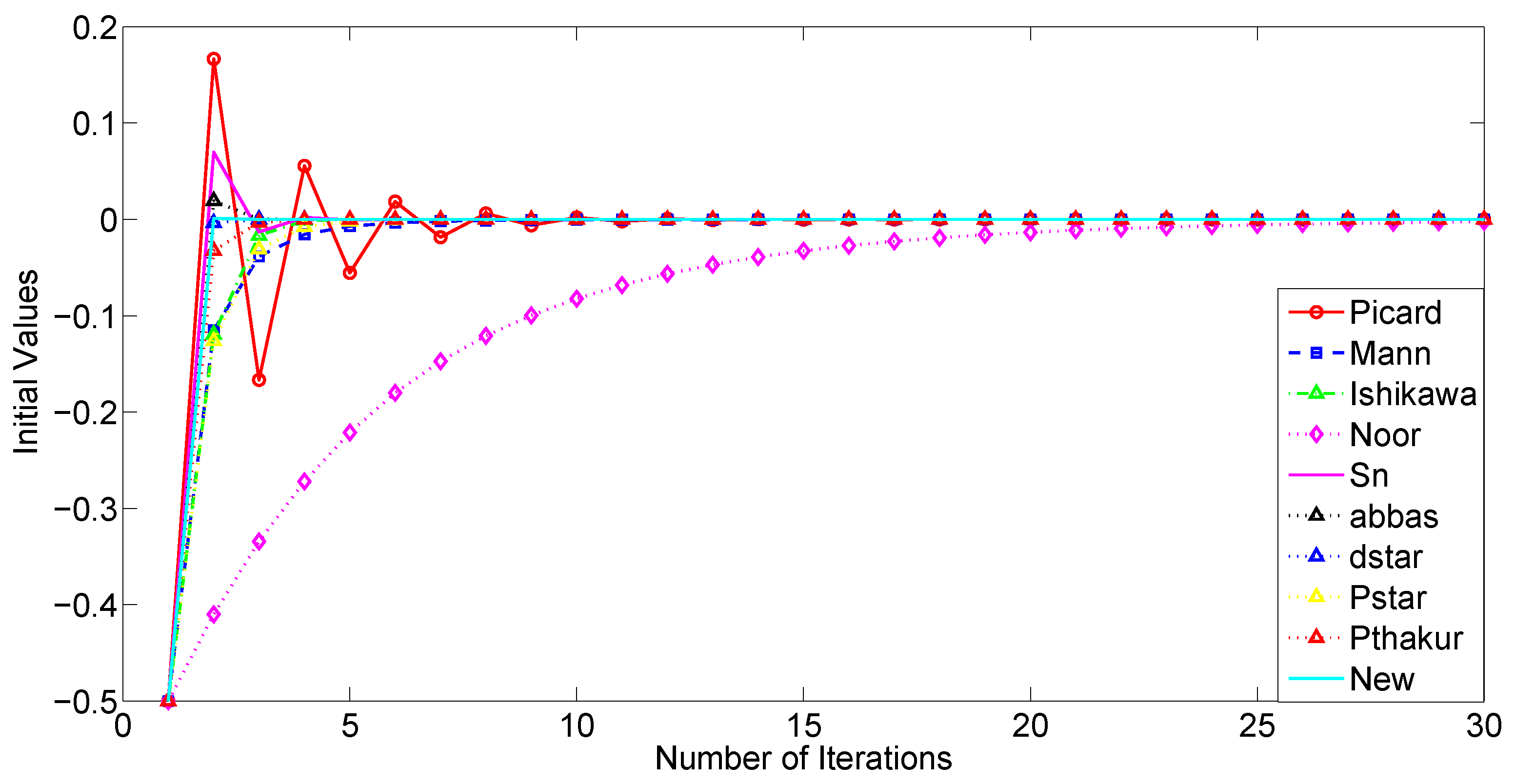
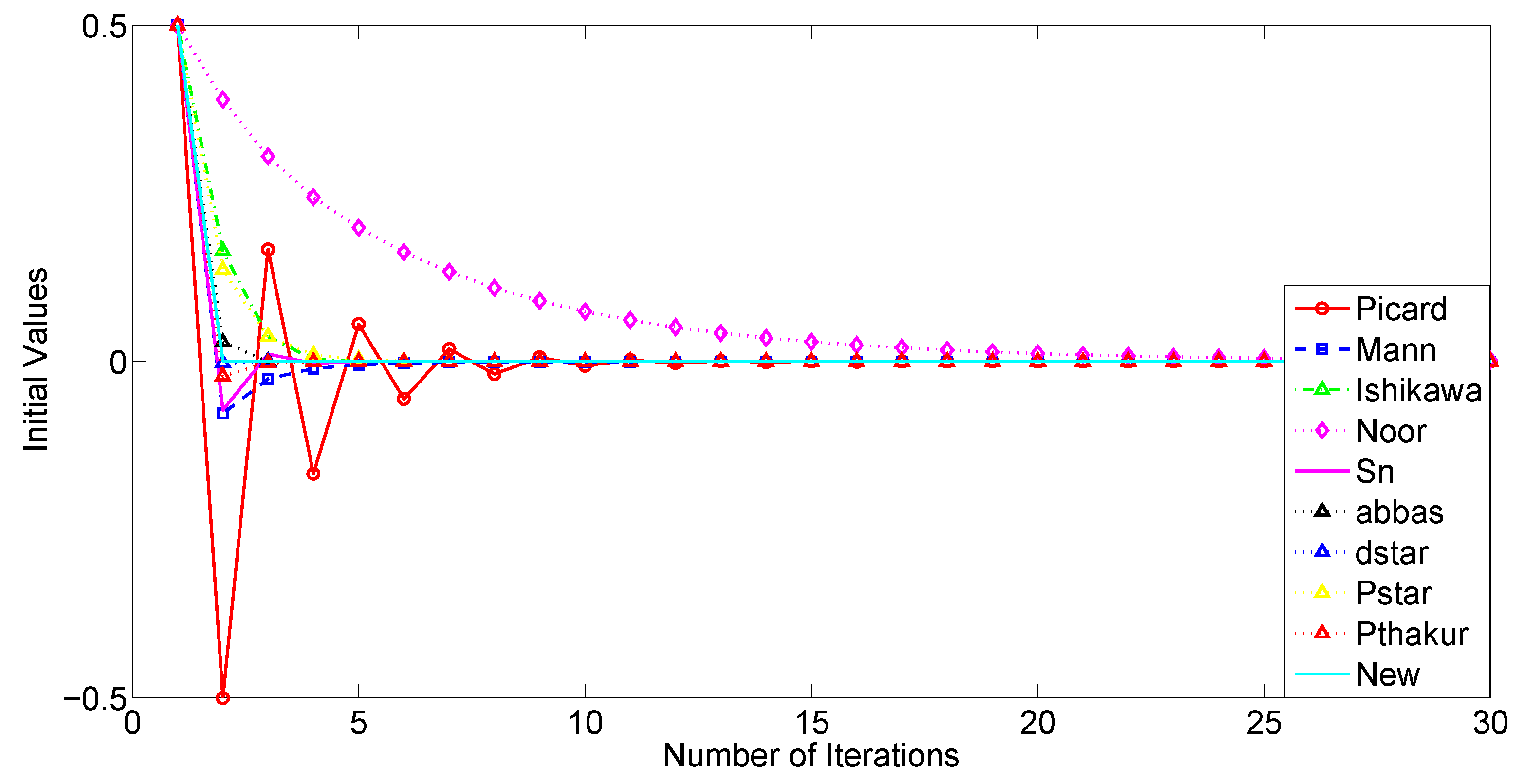
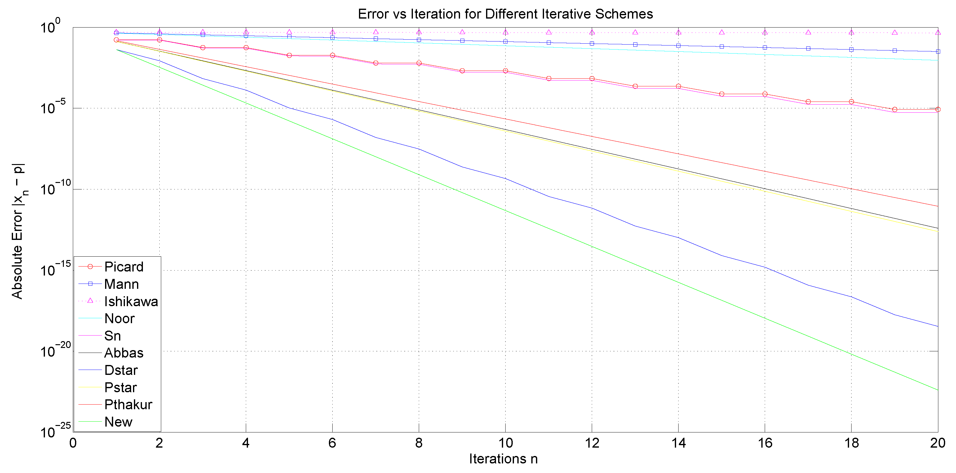
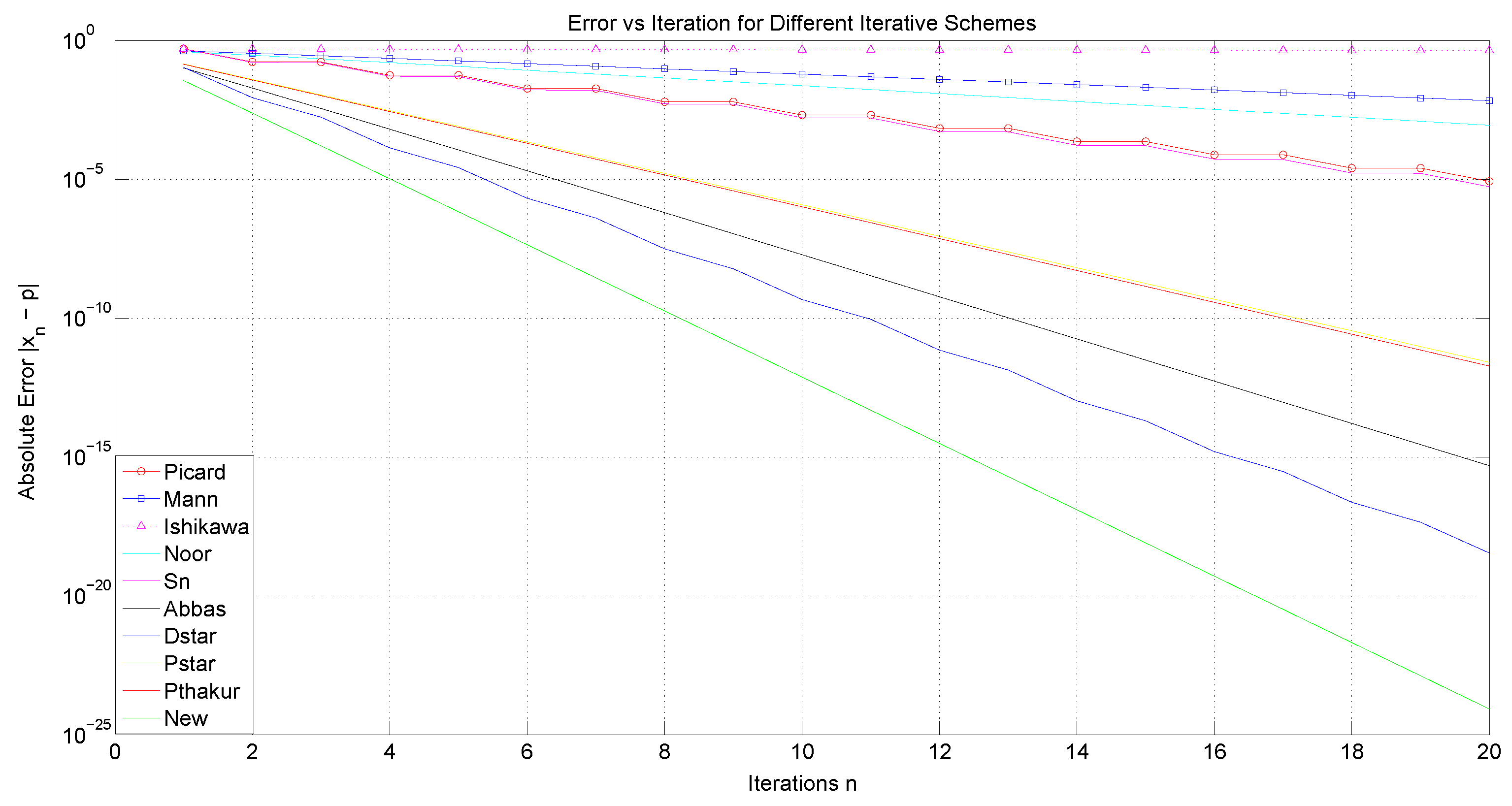
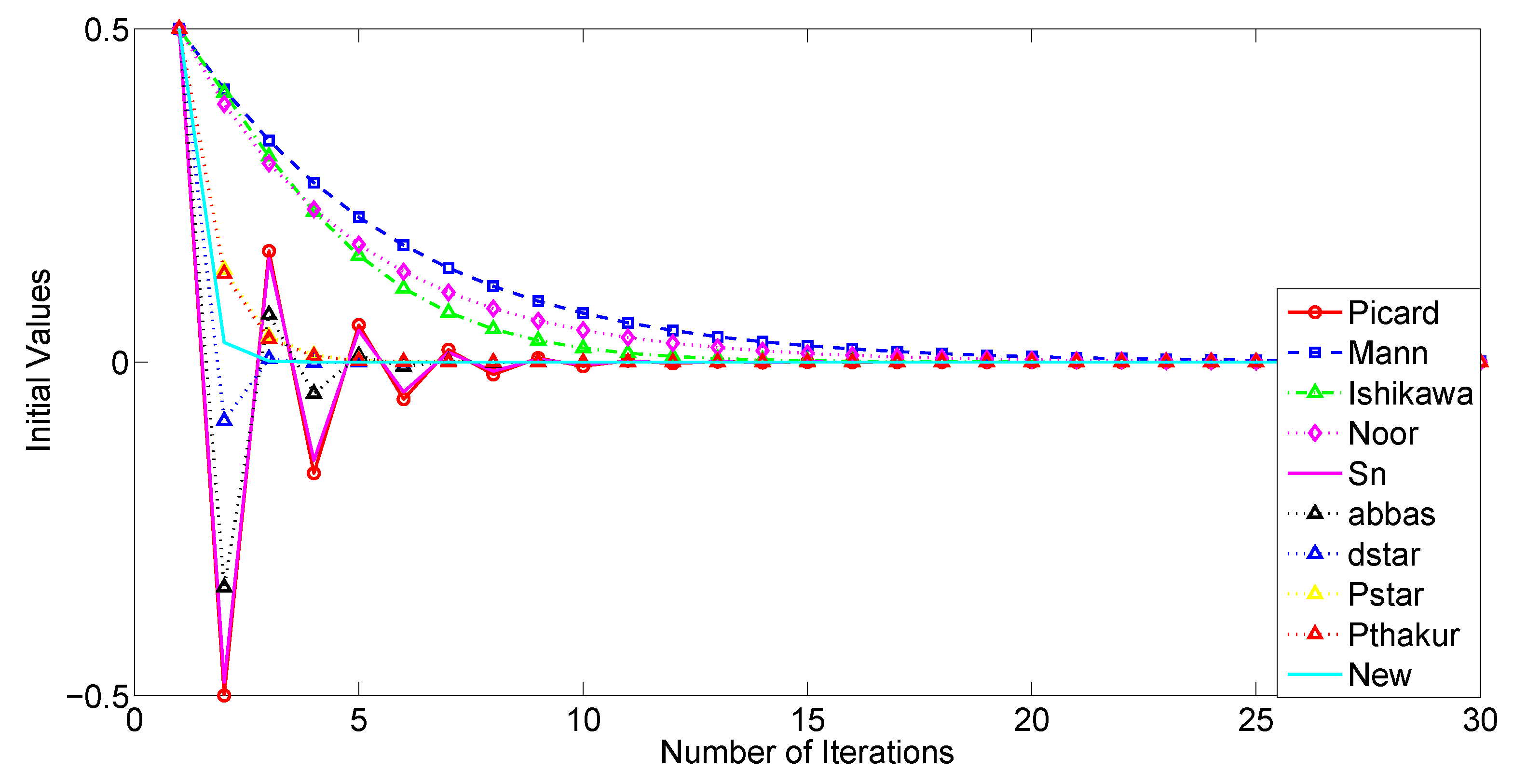
We now examine the convergence rates of several iteration processes, namely Picard, Mann, Ishikawa, Noor, Abbas, S n , D * , Picard S * , Picard–Thakur, and the new iteration (1) in the framework of Example 1 to compare their effectiveness and investigate the impact of different initial values on the convergence of these iteration schemes by varying the parameter α n , β n and γ n . Let p denote a fixed point of the mapping T. The stopping criterion is given by d ( x n , p ) < 10 12 .
As a starting point, our analysis will focus, on the one hand, on the convergence behavior of the iterative processes under consideration, and, on the other hand, on their computational aspects, such as execution time, the number of iterations required for convergence, and an estimation of the associated error. First, we shall use the sequences α n = n 10 n + 2 , β n = n ( 4 n + 11 ) 2 and γ n = n 7 n + 2 . Analogously to the preceding study, we will proceed by considering α n = 1 n + 1 , β n = n n + 2 and γ n = n 5 n + 2 .
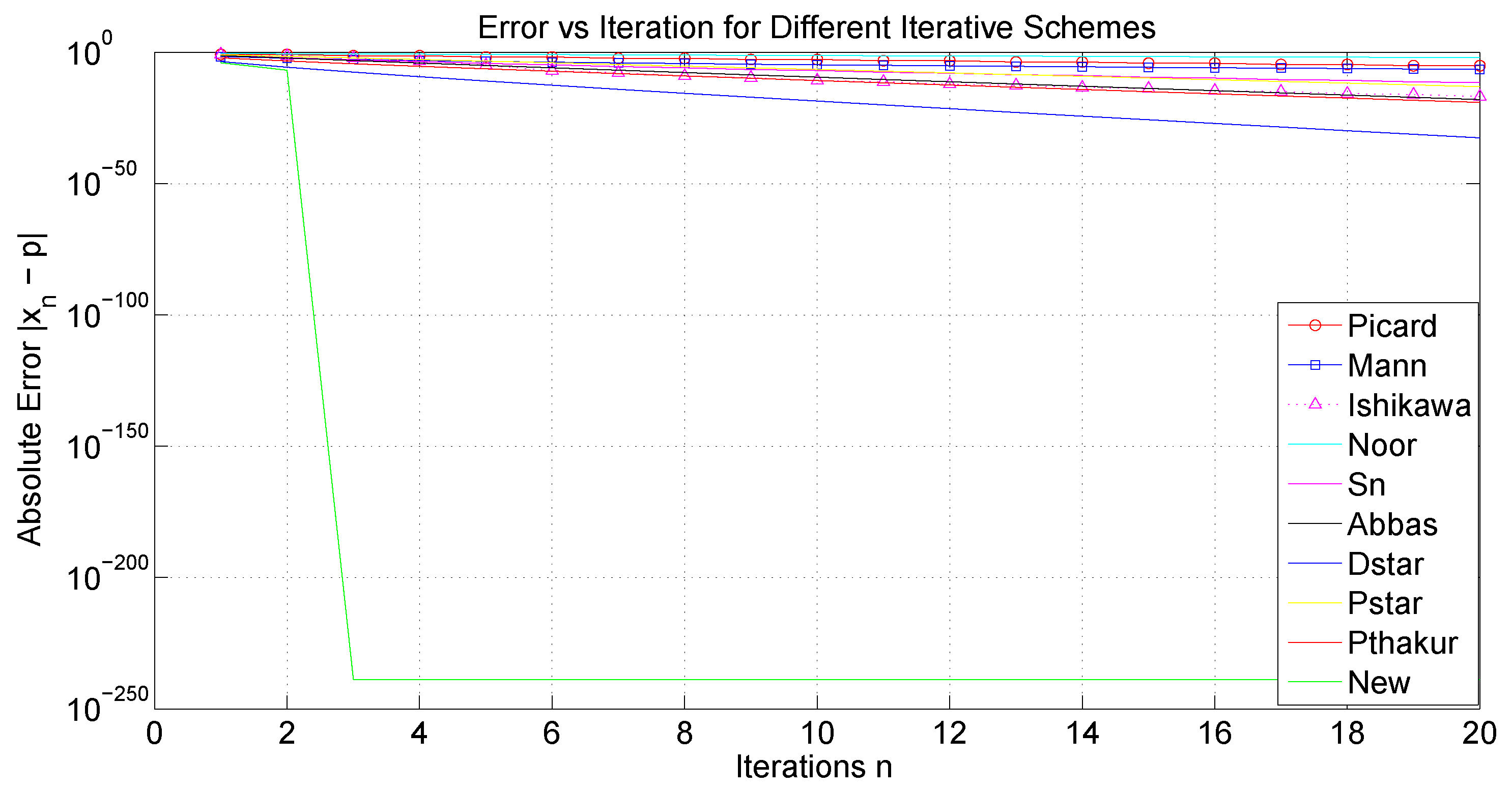
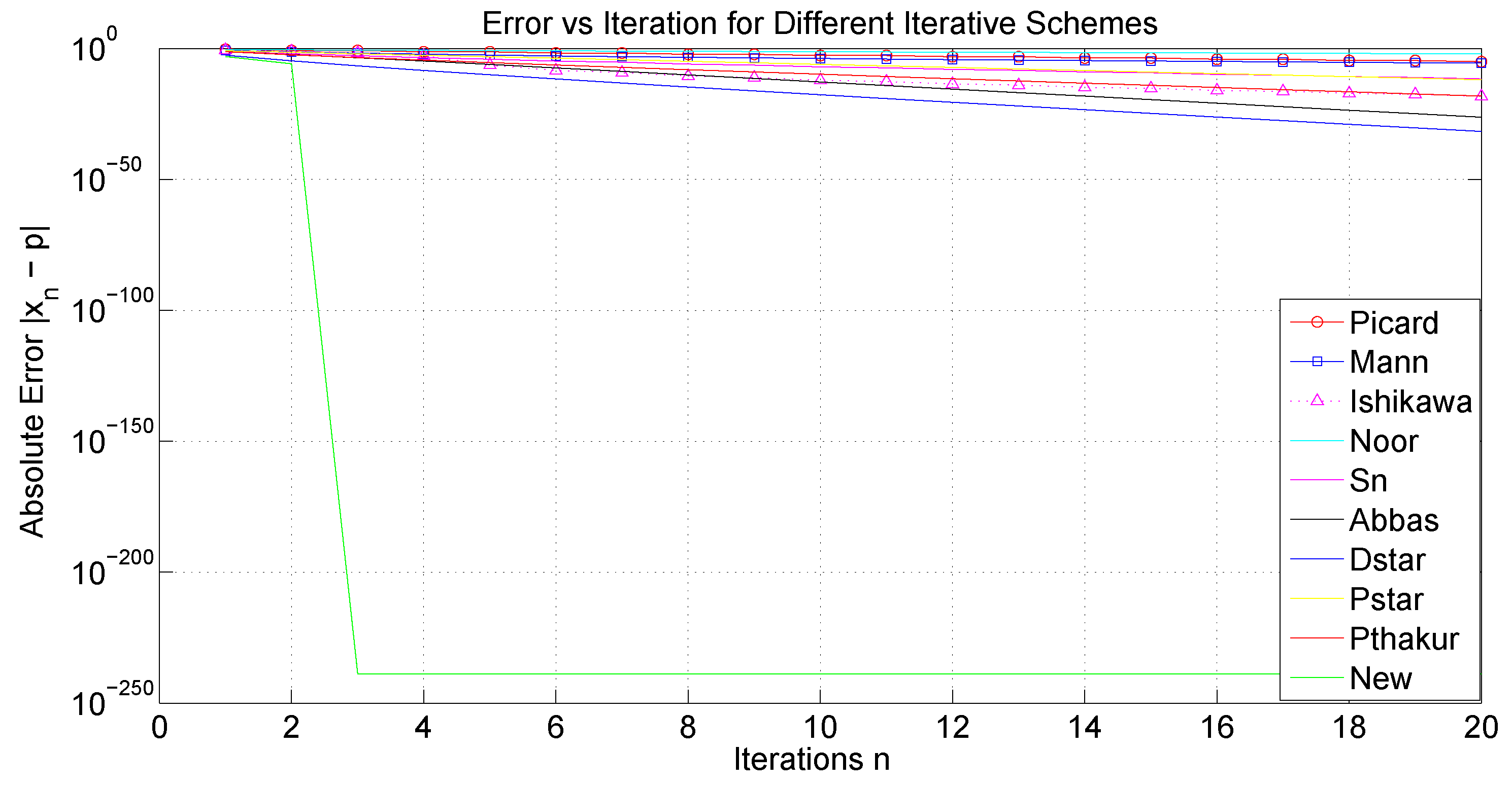
The tables and figures presented below illustrate a comprehensive comparison of the convergence behavior of the iterative schemes and demonstrate that, for different choices of parameters and initial guesses, our proposed iterative scheme (1) is more efficient and converges more rapidly to the fixed point of the mapping T. We have considered several choices of the initial point x 0 , as well as different sequences for { α n } , { β n } , and { γ n } , in order to emphasize that the efficiency of the proposed algorithm is not restricted to a single particular case. These variations indicate that the method remains effective under a wide range of parameter settings.
To strengthen the formulated conclusion, we emphasize the following points:
It is noteworthy that the three-step iterations, Abbas and D * , converge faster and are more efficient than the four-step iterations Picard S * and Picard–Thakur. This indicates that the convergence behavior of an iterative process is independent of the number of steps in which the process is defined.
Since the theoretical results were developed within the framework of CAT(0) spaces, we present a recently introduced example from the specialized literature, which also allows for a corresponding numerical simulation.
Example 2
([29]). Let us consider Poincaré half-plane
H = { x = ( x 1 , x 2 ) : x 1 , x 2 R , x 2 > 0 } ,
with the Poincaré metric
d ( x , y ) = 2 ln ( y 1 x 1 ) 2 + ( y 2 x 2 ) 2 + ( y 1 x 1 ) 2 + ( y 2 + x 2 ) 2 2 x 2 y 2 .
We consider the mapping
T : H H , T ( x 1 , x 2 ) = ( x 1 , x 2 ) .
Then, T is nonexpansive in connection with the hyperbolic distance d.
The goal here is to apply the iterative procedure (1) starting from a chosen initial estimate x 0 H to obtain the corresponding fixed point of T. To perform this, it is first necessary to have a clear understanding of how z = ( 1 t ) x t y can be computed exactly.
Given two points x = ( x 1 , x 2 ) , y = ( y 1 , y 2 ) H and a scalar t [ 0 , 1 ] , we aim to derive an explicit expression for z = ( 1 t ) x t y , i.e., the unique point on the geodesic segment between x and y, such that
d ( x , z ) = t d ( x , y ) .
According to [29], it has been proven that for two given points, x , y H and t ( 0 , 1 ) , one has
( 1 t ) x t y = ( p , x 2 1 t y 2 t ) , i f x 1 = y 1 = p ; a + R 1 λ 2 ( x , y , t ) 1 + λ 2 ( x , y , t ) , R 2 λ ( x , y , t ) 1 + λ 2 ( x , y , t ) , i f x 1 y 1 ,
where
a = ( y 1 2 + y 2 2 ) ( x 1 2 + x 2 2 ) 2 ( y 1 x 1 ) ,
R = ( y 1 x 1 ) 2 + ( y 2 x 2 ) 2 · ( y 1 x 1 ) 2 + ( y 2 + x 2 ) 2 2 | x 1 y 1 | ,
and
λ ( x , y , t ) = R + a x 1 x 2 1 t R + a y 1 y 2 t .
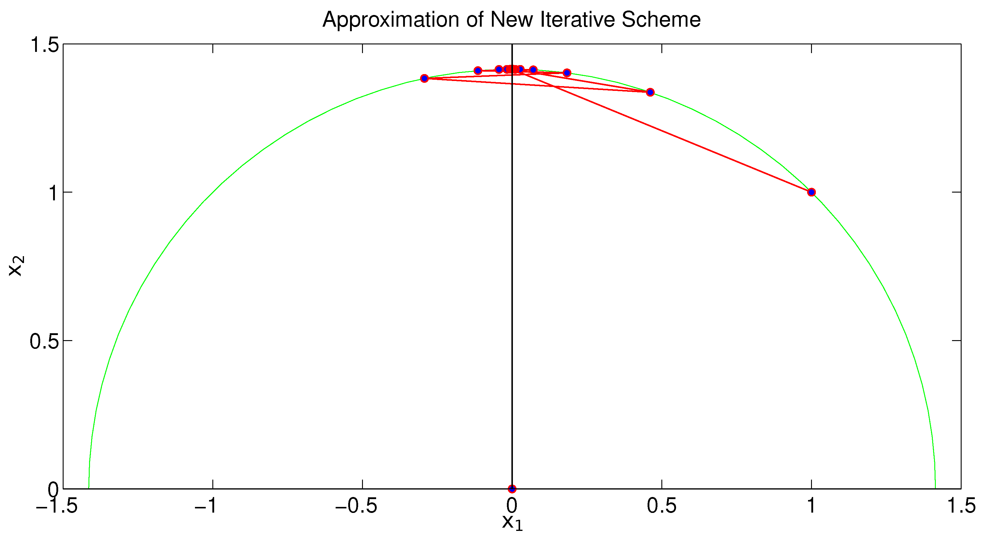
We now incorporate the formula derived above into the iterative scheme (1) to approximate the fixed point of the hyperbolic nonexpansive operator T. To illustrate this, we take the initial guess x 0 = ( 1 , 1 ) and set the permissible error to ε = 10 3 . The stopping condition for the algorithm is defined as d ( x n + 1 , x n ) < ε , where d denotes the Poincaré metric.
Figure 9 illustrates the approximate sequence { x n } from the initial guess to the computed solution. It is worth noting that the entire sequence lies on the geodesic connecting x 0 and x * (depicted as the green semicircle).

5. Application in Integral Equations

The theory of fixed points plays a central role in the study of integral equations, as it provides a powerful and unifying framework for establishing the existence, uniqueness, and stability of solutions. By reformulating integral equations as fixed point problems in appropriate functional spaces, one can apply a variety of fixed point theorems to analyze convergence properties and construct iterative methods. For instance, in [30], iterative numerical methods are developed to solve Fredholm–Hammerstein integral equations with modified arguments, highlighting the practical applicability of fixed point techniques in numerical analysis. In [31], the authors employ fixed point theory to perform a stability analysis of quadratic functional equations in quasi-Banach spaces, extending the reach of these methods beyond classical Banach spaces. A novel approach based on fixed points in F -bipolar metric spaces is proposed in [32], where Volterra integral equations are investigated from a fresh geometric perspective. The application of fixed point theorems to fractional boundary value problems in tempered sequence spaces is presented in [33], further illustrating the versatility of the method in dealing with infinite systems. Another recent contribution is [34], where the existence of solutions for Fredholm integral equations is established through a fixed point framework, underscoring the fundamental role of this theory in both the qualitative and quantitative study of integral equations. In what follows, we shall employ the proposed iterative process for solving a Fredholm integral equation.
Let C [ a , b ] be the space of all continuous functions equipped with a metric induced by the norm
x y = sup t [ a , b ] | x ( t ) y ( t ) | , x , y C [ a , b ] .
Consider the following Fredholm integral equation:
x ( t ) = ϕ ( t ) + a b K ( t , s ) f ( t , s , x ( s ) ) d s .
Suppose the following assumptions holds:
i.
Let ϕ : [ a , b ] R be continuous.
ii.
The kernal K : [ a , b ] 2 R is continuous and satisfies
| K ( t , s ) | 1 .
iii.
The function f : [ a , b ] 2 × R R is continuous and the following holds:
| f ( t , s , x ( s ) ) f ( t , s , y ( s ) ) | | x ( t ) y ( t ) | a b , t [ a , b ] .
Define the mapping T : C [ a , b ] C [ a , b ] by
T x ( t ) = ϕ ( t ) + a b K ( t , s ) f ( t , s , x ( s ) ) d s .
Theorem 10.
Under the above assumptions, the integral equation given by (10) has a solution and the sequence defined by (1) converges to the solution.
Proof. 
Using the assumptions, we get
| x ( t ) T y ( t ) | | x ( t ) T x ( t ) | + | T x ( t ) T y ( t ) | = | x ( t ) T x ( t ) | + | ϕ ( t ) + a b K ( t , s ) f ( t , s , x ( s ) ) d s ϕ ( t ) a b K ( t , s ) f ( t , s , y ( s ) ) d s | = | x ( t ) T x ( t ) | + a b K ( t , s ) f ( t , s , x ( s ) ) d s a b K ( t , s ) f ( t , s , y ( s ) ) d s | x ( t ) T x ( t ) | + a b | K ( t , s ) | | f ( t , s , x ( s ) ) f ( t , s , y ( s ) ) | d s | x ( t ) T x ( t ) | + a b | x ( t ) y ( t ) | b a d s | x ( t ) T x ( t ) | + | x ( t ) y ( t ) | .
By taking the supremum, we obtain
sup t [ a , b ] | x ( t ) T y ( t ) | sup t [ a , b ] | x ( t ) T x ( t ) | + sup t [ a , b ] | x ( t ) y ( t ) | ,
so
x T y   x T x + x y .
Therefore, mapping T satisfies condition ( E ) , with μ 1 . By Theorem 1, the sequence defined by (1) converges to the solution of integral Equation (10). □
Example 3.
Let C [ 0 , 1 ] be the space of all continuous functions with a metric defined as
x y = sup t [ a , b ] | x ( t ) y ( t ) | , x , y C [ 0 , 1 ] .
Consider the following first-order initial value problem:
x = t x ( t ) 2 t , x ( 0 ) = 0 .
The existence of a solution of (11) is equivalent to finding a fixed point of the integral operator, defined as
T x ( t ) = x ( 0 ) + 0 t s x ( s ) 2 s d s .
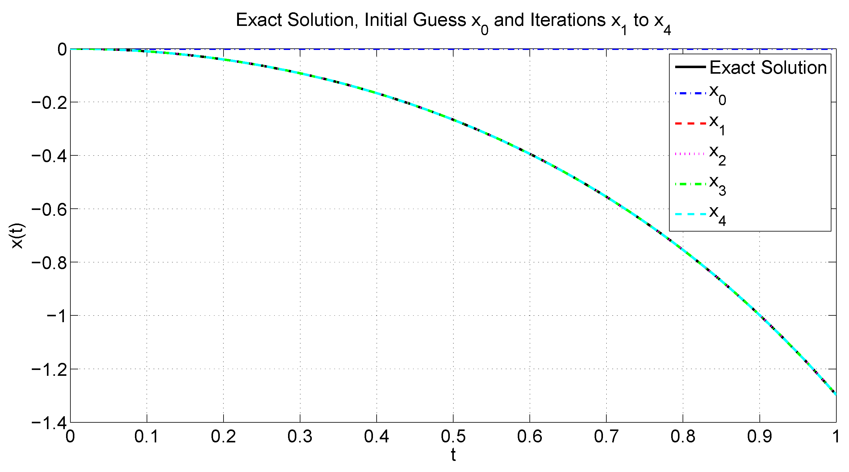
It can be easily shown that this operator satisfies the Garcia–Falset property and has a fixed point g ( t ) = 2 1 e t 2 2 in C [ 0 , 1 ] . By Theorem 10, the iterative algorithm (1) generated by T converges to g ( t ) . For the initial guess x 0 ( t ) = 0 and choices of parameters α n = 1 n + 1 , β n = n n + 2 and γ n = n 7 n + 2 . Figure 10 and Figure 11 compare the exact solution to the approximate solutions obtained using a new method. At first glance, the new solutions seem almost identical to the exact one. However, upon closer inspection, tiny differences become apparent. These small deviations indicate that while the new method is highly precise, there is a minimal numerical error involved. Despite this, the close agreement between the exact and new solutions demonstrates the effectiveness and reliability of the proposed approach, making it an appropriate method for solving such problems.

6. Comparison via Polynomiography

In this section, we shift our perspective and highlight an alternative application of the new iteration procedure. Consider a nonconstant polynomial p, defined on the closed unit disk D = z C : | z | 1 . According to the Maximum Modulus Principle, the largest value of the modulus, denoted by
p = max z D | p ( z ) |
is always attained at one or more points located on the boundary of D.
A significant contribution in this direction was made by Kalantari in [35], where he proposed a novel approach to the problem of maximizing the modulus of complex polynomials. Specifically, his work introduced a reformulation of the problem, first by expressing it as a fixed point problem and subsequently by reducing it to the search for roots of a suitably defined pseudo-polynomial. This methodological shift opened the way to new computational strategies, and it is grounded in the fundamental equivalence stated below.
Theorem 11
([35]). Let p ( z ) be a nonconstant polynomial on D = z C : | z | 1 . A point z * D is a local maximum of | p ( z ) | over D if and only if
z * = F ( z * ) ,
where
F ( z ) = p ( z ) p ( z ) / | p ( z ) p ( z ) | ,
meaning that it finds itself among the solutions of the zero-search problem
G ( z * ) = 0 ,
where
G ( z ) = p ( z ) | p ( z ) | z p ( z ) | p ( z ) | .
Further, we extend our analysis by combining the newly introduced iteration procedure with specific elements drawn from the so-called Basic Family of Iterations, suitably adapted to the sequence of functions { G n ( z ) } . More precisely, our focus will be on the first three members of the Basic Family, together with the associated sequences of iteration functions derived within the framework of the Maximum Modulus Principle (MMP):
( B 2   or   pseudo - Newton ) B 2 , n ( z ) = N n ( z ) = z G n ( z ) G n ( z ) ( B 3   or   pseudo - Halley ) B 3 , n ( z ) = H n ( z ) = z 2 G n ( z ) G n ( z ) 2 G n ( z ) 2 G n ( z ) G n ( z ) ( B 4 ) B 4 , n ( z ) = z 6 G n ( z ) 2 G n ( z ) 3 G n ( z ) G n ( z ) 2 G n ( z ) G n ( z ) 2 + 6 G n ( z ) 3 6 G n ( z ) G n ( z ) G n ( z ) .
If T n indicates any of the MMP iteration functions listed above, then the resulting New-MMP procedure is
w n = T n ( 1 α n ) x n + α n T n x n z n = T n ( 1 β n ) w n + β n T n w n y n = T n ( 1 γ n ) z n + γ n T n z n x n + 1 = T n y n ,
for all n 1 , where { α n } , { β n } , and { γ n } are real sequences in 0 , 1 .
Inspired by the fact that several recent studies suggest, based on polynomiographic applications, that the iterative process employed is more efficient (see, for instance, [36,37,38]), we now proceed with a more detailed analysis from this perspective. Our aim is to examine how these iterative schemes perform in practice and what insights can be gained from their visual representation. To set the stage for this discussion, we begin by clarifying several aspects related to the interpretation of the images presented in the following section.
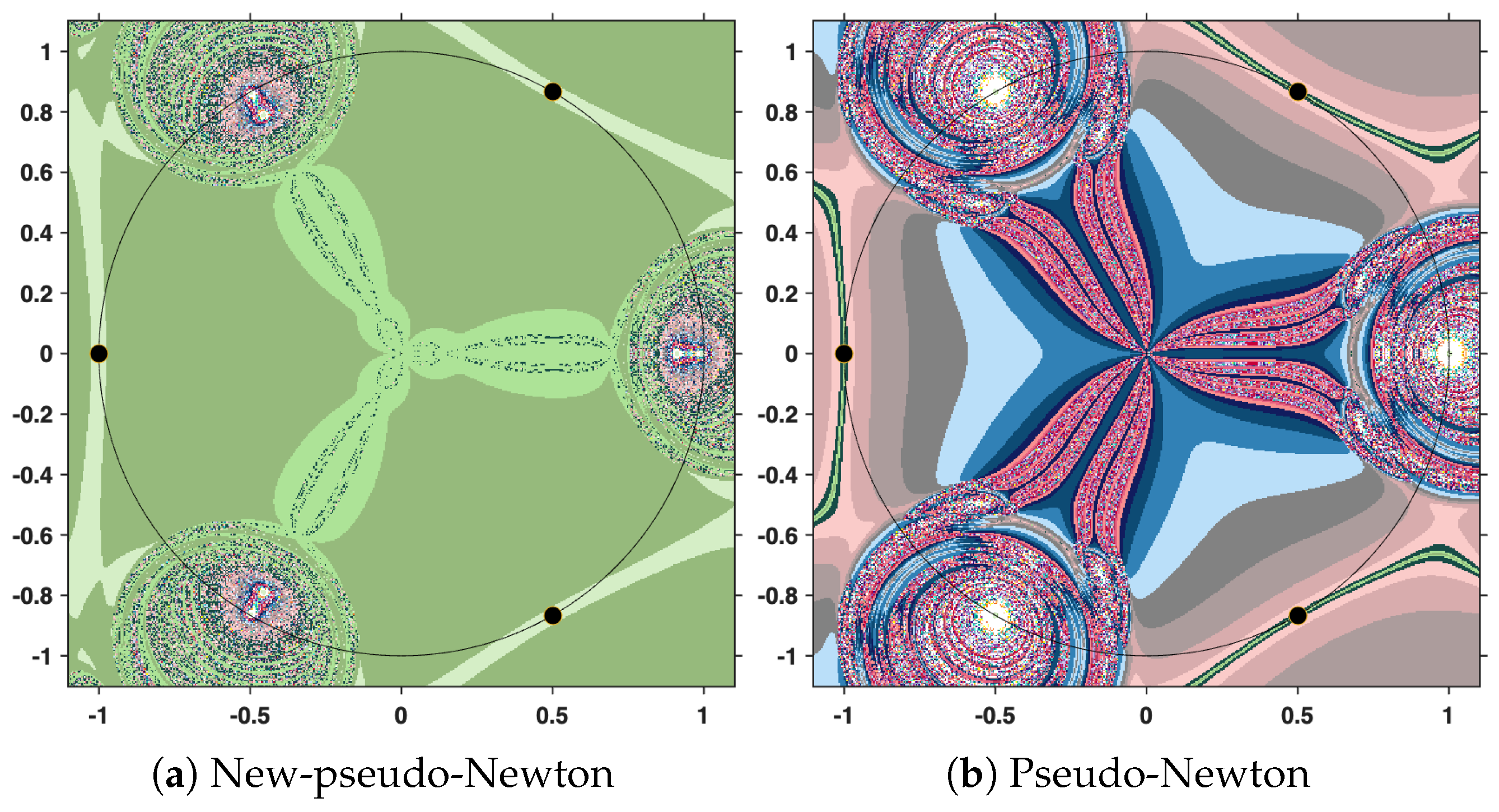
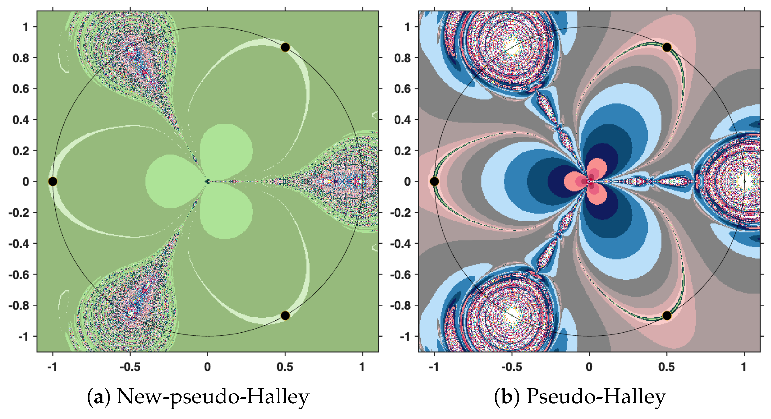
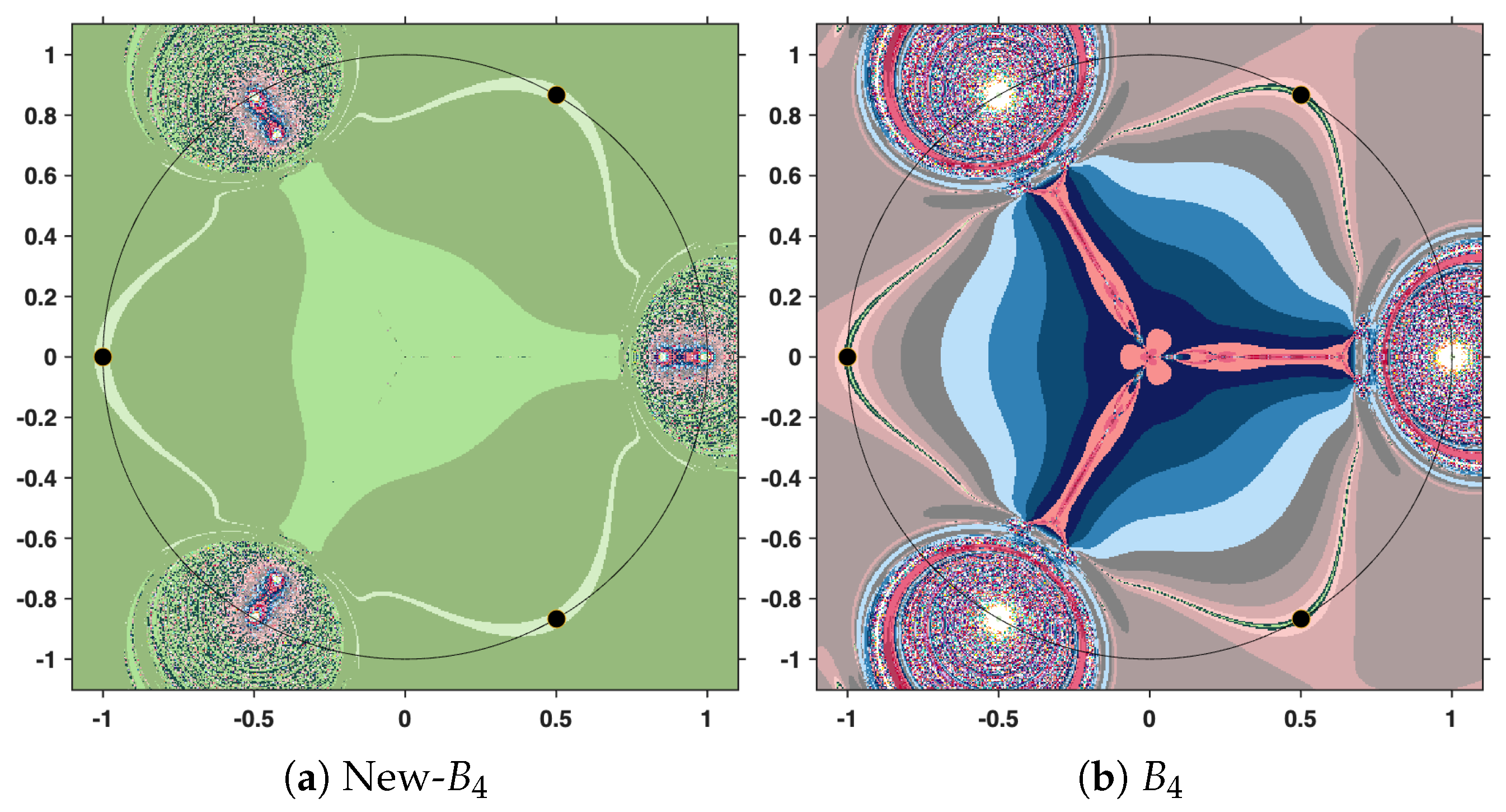
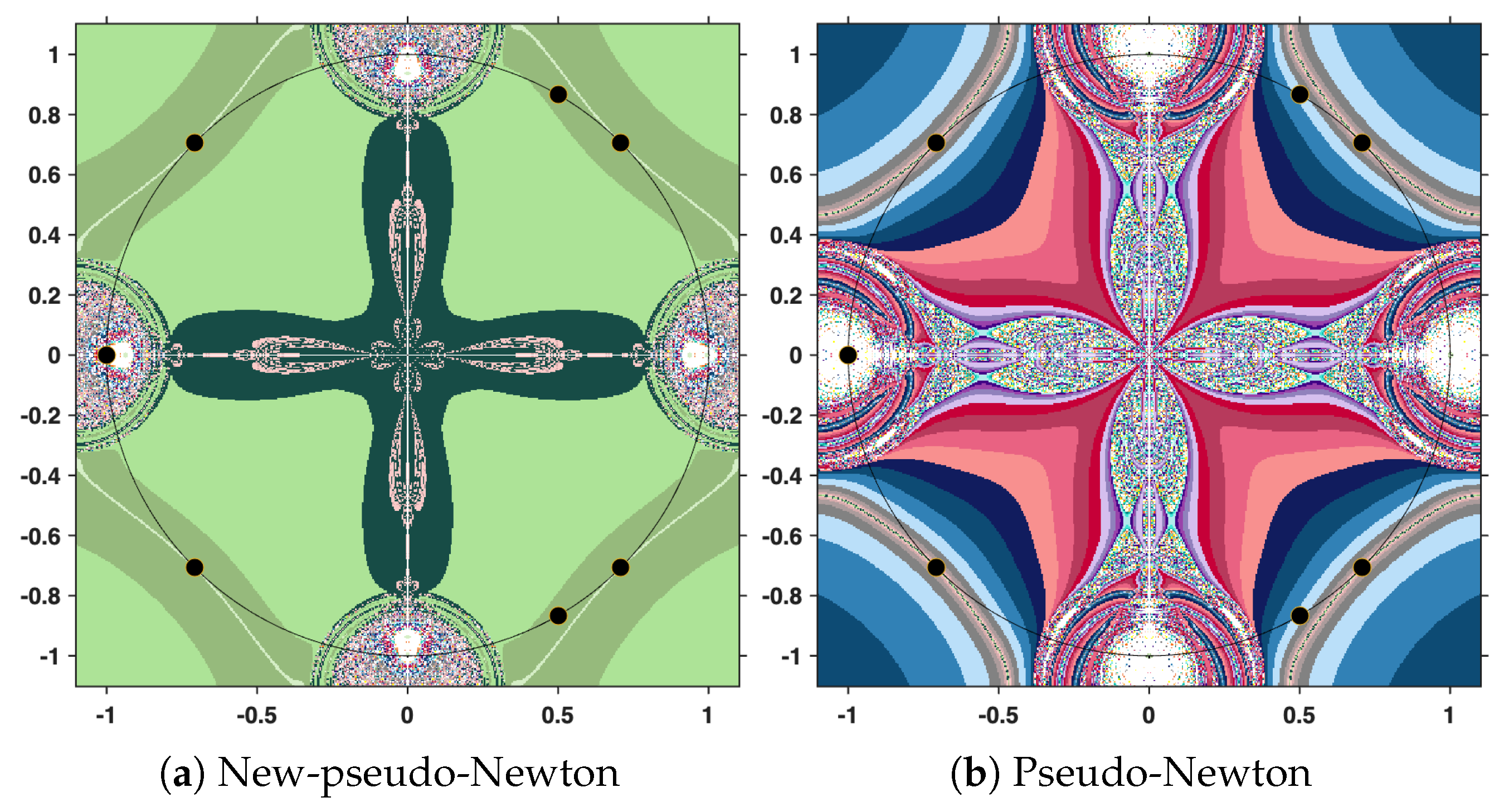
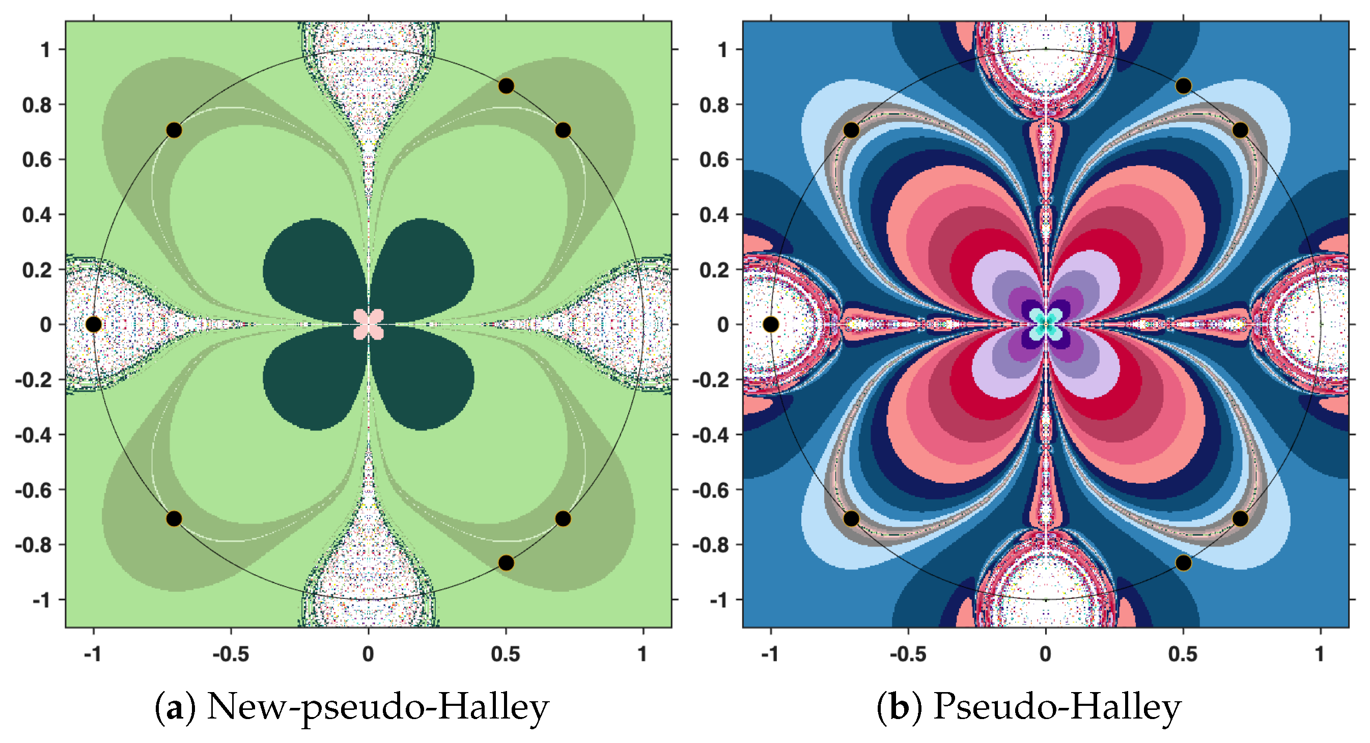
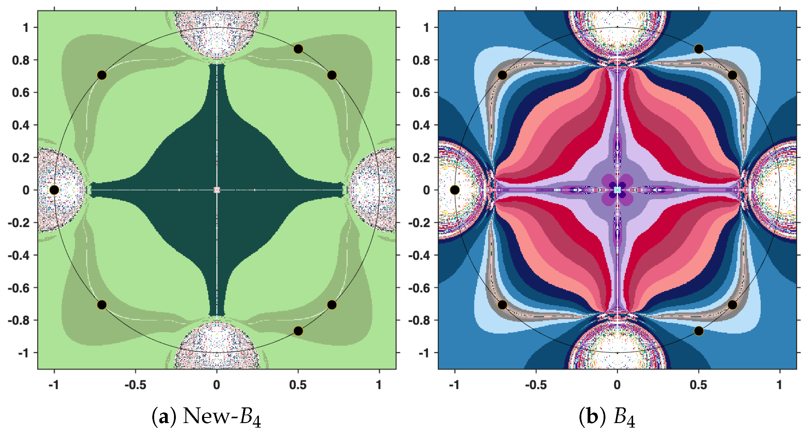
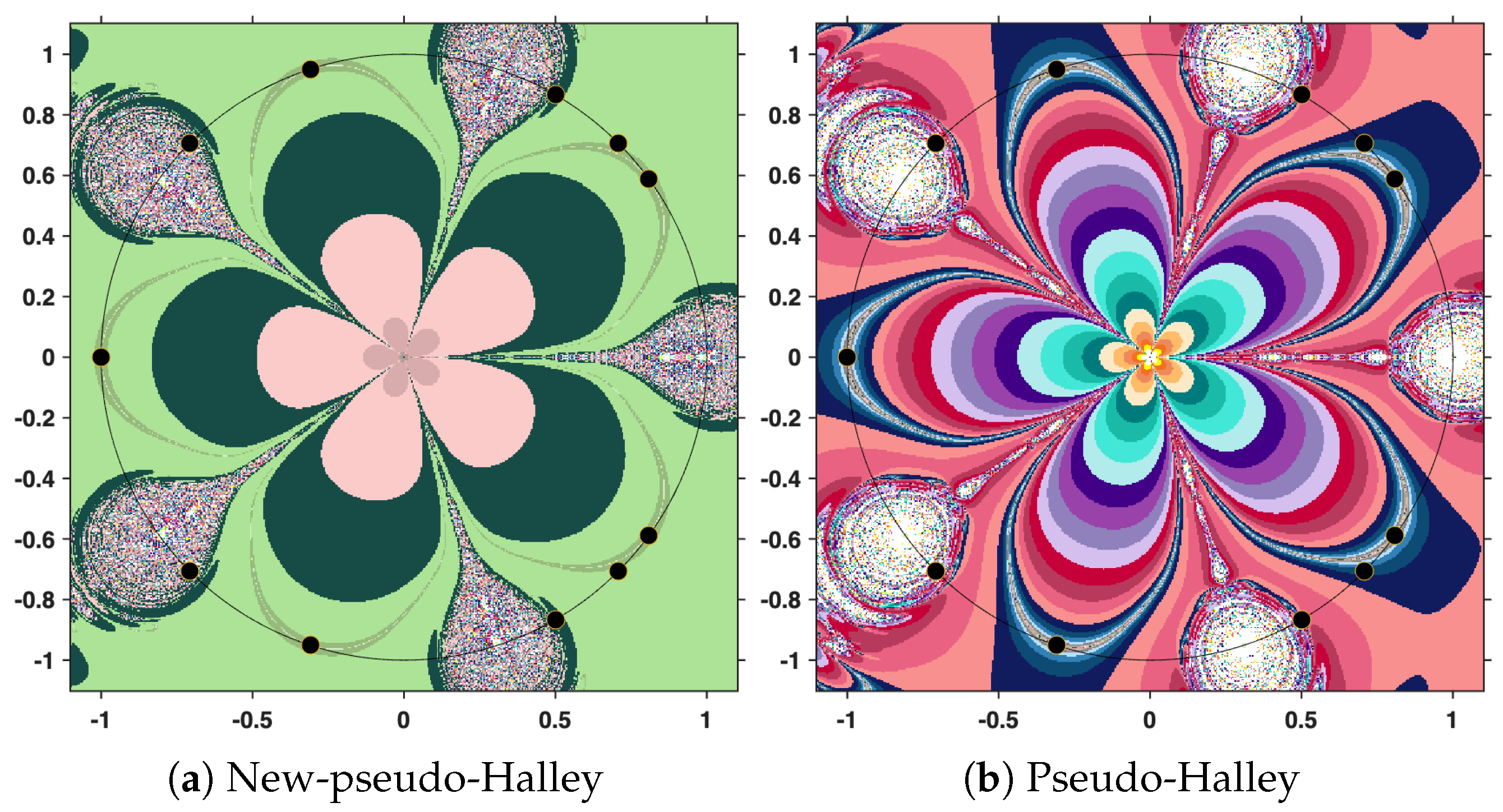
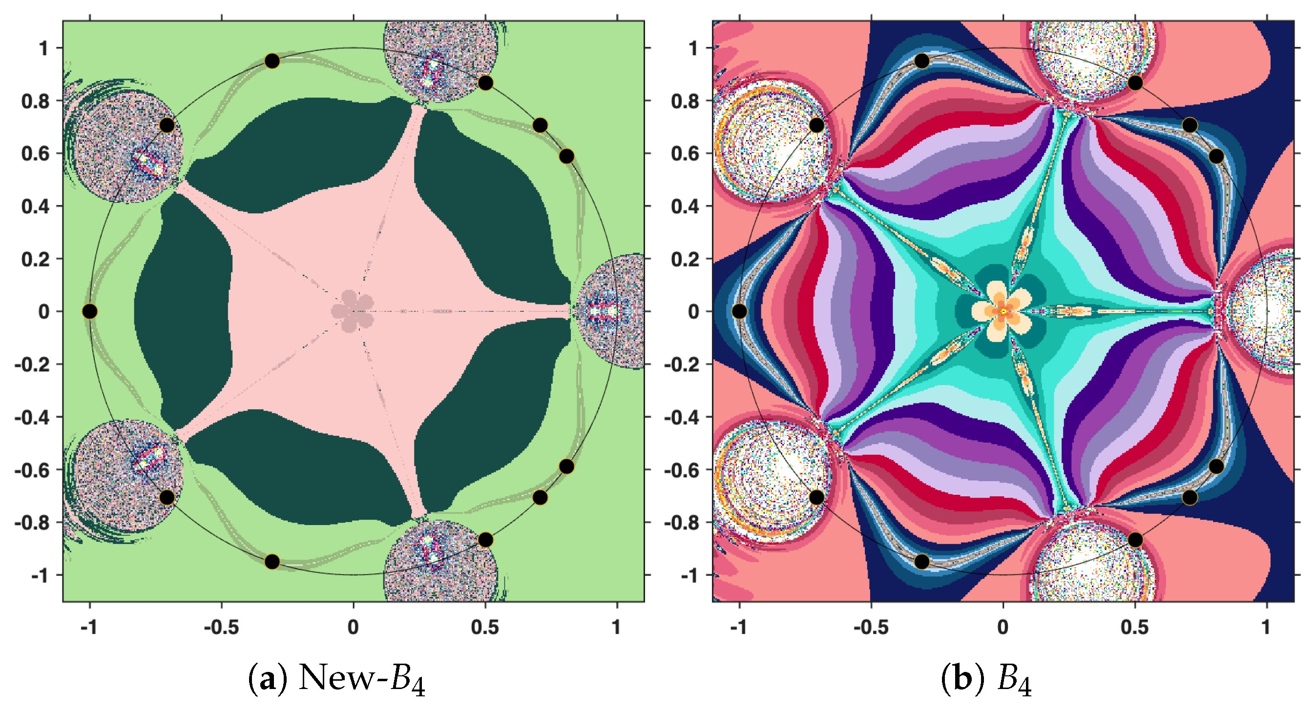
The output of the numerical algorithm is a colored picture (named polynomiograph), emphasizing the behavior of orbits. The black points indicate precisely the solutions, while white points mark the inefficient initial estimates. All the other colors in the color palette present information about a particular length of the orbit. There is an obvious difference in color intensity when comparing a procedure based on the new iteration with the corresponding standard procedure. More precisely, less intense colors indicate shorter orbits, hence a more efficient algorithm. For clarity, the legend of the colors used is shown in Figure 12.
In the subsequent analysis, we employ the New-MMP procedures in order to compute the maximum modulus of the complex polynomial p ( z ) = z 3 1 . For the sake of comparison, we also implement the classical MMP procedures, which are formulated on the basis of Picard iteration. The execution of these numerical algorithms requires, as a first step, the specification of the iteration step sizes. In our case, the parameters are set to α n = 1 3 , β n = 1 5 and γ n = 4 5 . It should be emphasized that this selection is purely arbitrary and does not rely on a particular theoretical justification; the purpose is simply to illustrate the performance of the methods under a fixed set of numerical values.
In addition to the step sizes, it is necessary to establish clear termination criteria for the iterative scheme. To this end, two stopping conditions are introduced. The first is a tolerance threshold for the error, which we set at ε = 10 4 . This ensures that the procedure terminates once two successive iterates in the orbit become sufficiently close, thus providing a guarantee of numerical accuracy. The second condition is a maximal number of iterations, fixed at K = 31 . This serves as a safeguard against divergence or excessively long computations, preventing the algorithm from running indefinitely.
Therefore, the iterative construction will be terminated as soon as at least one of these conditions is satisfied: either the distance between two consecutive elements of the orbit falls below the prescribed tolerance, or the orbit has been extended to the limit of 31 iterations. In this way, the process balances both accuracy and computational efficiency, while allowing a fair comparison between the New-MMP and the classical MMP procedures. The resulting polynomiographs are pictured in Figure 13, Figure 14 and Figure 15.
This time, we employ the same parameters, the same stopping criterion, and the same maximum number of iterations as in the previous experiment. However, instead of the cubic polynomial, we now consider the complex polynomial p ( z ) = z 4 1 . The purpose of this change is to examine how the methods perform when applied to a polynomial of higher degree, while maintaining identical computational settings. The resulting polynomiographs are pictured in Figure 16, Figure 17 and Figure 18.
Finally, under the same conditions specified above, but this time considering the complex polynomial p ( z ) = z 5 1 , we obtain the graphical results shown in Figure 19, Figure 20 and Figure 21.
To strengthen the efficiency of the newly introduced iterative process, we will present an objective method of analysis in the case of using the polynomial p ( z ) = z 5 1 , by employing an indicator which we will denote as PD(10). This indicator measures the percentage of the considered domain for which the iterative sequence reaches an approximation error smaller than 10 4 within at most 10 iterations. The results are presented in Table 13.
It should be emphasized that the better performance presented in Table 13 is evaluated specifically for an approximation error of 10 4 within the first 10 iterations, the choice of the maximum number of iterations being arbitrary. While this comparison is limited to these parameters, the results still illustrate the method’s overall efficiency and robustness compared to classical iterative methods.

7. Conclusions

With a focus on investigating convergence results within the framework of spaces with nonlinear structures, we propose a novel iterative scheme for approximating the fixed points of a class of mappings satisfying Garcia–Falset property. Using this new method, we establish several existence and convergence results that extend and unify known results from linear spaces to nonlinear CAT(0) spaces. We also analyze the stability and data dependence of the proposed iterative scheme. Furthermore, numerical experiments, including an analysis of error values, computational time, and the number of iterations, show that our approach is more effective and achieves a quicker error reduction in the initial steps compared to classical iterative schemes. These results are observed within the first few steps and provide an indication of the method’s practical efficiency, without making claims about the full convergence behavior. Finally, we apply the new results to the solution of an integral equation and explore the newly introduced iterative process from the perspective of polynomiography. As a natural continuation of the present work, one may undertake a rigorous analysis of the newly introduced iterative process within the broader framework of hyperbolic spaces. Such an investigation could parallel, for instance, the approach in [39], where convergence properties are examined, or that in [40], where stability and data dependence are addressed for a three-step iterative scheme.

Author Contributions

Conceptualization, M.K., M.A. and C.C.; software, M.K. and C.C.; validation, M.A. and C.C.; formal analysis, C.C.; writing—original draft preparation, M.K.; writing—review and editing, M.K., M.A. and C.C.; supervision, M.A. All authors have read and agreed to the published version of the manuscript.

Funding

This work was supported by a grant from the National Program for Research of the National Association of Technical Universities—GNAC ARUT 2023.

Data Availability Statement

The original contributions presented in this study are included in the article. Further inquiries can be directed to the corresponding author.

Conflicts of Interest

The authors declare no conflicts of interest.

References

  1. Bridson, M.R.; Haefliger, A. Metric Spaces of Non-Positive Curvature; Springer: Berlin/Heidelberg, Germany, 1999. [Google Scholar]
  2. Dhompongsa, S.; Panyanak, B. On Δ-convergence theorems in CAT(0) spaces. Comput. Math. Appl. 2008, 56, 2572–2579. [Google Scholar] [CrossRef]
  3. Laowang, W.; Panyanak, B. Approximating fixed points of nonexpansive nonself mappings in CAT(0) spaces. Fixed Point Theory Appl. 2009, 2010, 367274. [Google Scholar] [CrossRef]
  4. Senter, H.F.; Dotson, W.G. Approximating fixed points of nonexpansive mappings. Proc. Am. Math. Soc. 1974, 44, 375–380. [Google Scholar] [CrossRef]
  5. Suzuki, T. Fixed point theorems and convergence theorems for some generalized nonexpansive mappings. J. Math. Anal. Appl. 2008, 340, 1088–1095. [Google Scholar] [CrossRef]
  6. García-Falset, J.; Llorens-Fuster, E.; Suzuki, T. Fixed point theory for a class of generalized nonexpansive mappings. J. Math. Anal. Appl. 2011, 375, 185–195. [Google Scholar] [CrossRef]
  7. Browder, F.E. Fixed-point theorems for noncompact mappings in Hilbert space. Proc. Natl. Acad. Sci. USA 1965, 53, 1272–1276. [Google Scholar] [CrossRef]
  8. Göhde, D. Zum Prinzip der kontraktiven Abbildung. Math. Nachr. 1965, 30, 251–258. [Google Scholar] [CrossRef]
  9. Kirk, W.A. A fixed point theorem for mappings which do not increase distances. Am. Math. Mon. 1965, 72, 1004–1006. [Google Scholar] [CrossRef]
  10. Kannan, R. Fixed point theorems in reflexive Banach spaces. Proc. Am. Math. Soc. 1973, 38, 111–118. [Google Scholar] [CrossRef]
  11. Gregus, M. A fixed point theorem in Banach spaces. Boll. Un. Mat. Ital. 1980, 17, 193–198. [Google Scholar]
  12. Aoyama, K.; Kohsaka, F. Fixed point theorem for α-nonexpansive mappings in Banach spaces. Nonlinear Anal. 2011, 74, 4387–4391. [Google Scholar] [CrossRef]
  13. Pant, R.; Shukla, R. Approximating fixed points of generalized α-nonexpansive mappings in Banach spaces. Numer. Funct. Anal. Optim. 2017, 38, 248–266. [Google Scholar] [CrossRef]
  14. Pandey, R.; Pant, R.; Rakocevic, V.; Shukla, R. Approximating fixed points of a general class of nonexpansive mappings in Banach spaces with applications. Results Math. 2019, 74, 7. [Google Scholar] [CrossRef]
  15. Karapinar, E. Remarks on Suzuki (C)-condition. In Dynamical Systems and Methods; Springer: New York, NY, USA, 2012; pp. 221–229. [Google Scholar]
  16. Bejenaru, A.; Postolache, M. A unifying approach for some nonexpansiveness conditions on modular vector spaces. Nonlinear Anal. Model. Control 2020, 25, 827–845. [Google Scholar] [CrossRef]
  17. Picard, É. Mémoire sur la théorie des équations aux dérivées partielles et la méthode des approximations successives. J. Math. Pure Appl. 1890, 6, 145–210. [Google Scholar]
  18. Mann, W.R. Mean value methods in iteration. Proc. Am. Math. Soc. 1953, 4, 506–510. [Google Scholar] [CrossRef]
  19. Ishikawa, S. Fixed points by a new iteration method. Proc. Am. Math. Soc. 1974, 44, 147–150. [Google Scholar] [CrossRef]
  20. Noor, M.A. New approximation schemes for general variational inequalities. J. Math. Anal. Appl. 2000, 251, 217–229. [Google Scholar] [CrossRef]
  21. Abbas, M.; Nazir, T. A new faster iteration process applied to constrained minimization and feasibility problems. Mat. Vesn. 2014, 66, 223–234. [Google Scholar]
  22. Sintunavarat, W.; Pitea, A. On a new iteration scheme for numerical reckoning fixed points of Berinde mappings with convergence analysis. J. Nonlinear Sci. Appl. 2016, 9, 2553–2562. [Google Scholar] [CrossRef]
  23. Hussain, A.; Ali, D.; Albargi, A.H. On assessing convergence and stability of a novel iterative method for fixed-point problems. AIMS Math. 2025, 10, 15333–15357. [Google Scholar] [CrossRef]
  24. Lamba, P.; Panwar, A. A Picard S* iterative algorithm for approximating fixed points of generalized α-nonexpansive mappings. J. Math. Comput. Sci. 2021, 11, 2874–2892. [Google Scholar] [CrossRef]
  25. Jia, J.; Zhang, X.; Li, Y.; Wang, Z. Strong convergence of a new hybrid iterative scheme for nonexpansive mappings and applications. J. Funct. Spaces 2022, 2022, 4855173. [Google Scholar]
  26. Harder, A.M. Fixed Point Theory and Stability Results for Fixed Point Iteration Procedures. Ph.D. Thesis, University of Missouri-Rolla, Rolla, MO, USA, 1987. [Google Scholar]
  27. Haghi, R.H.; Postolache, M.; Rezapour, S. On T-stability of the Picard iteration for generalized φ-contraction mappings. Abstr. Appl. Anal. 2012, 2012, 658971. [Google Scholar] [CrossRef]
  28. Weng, X. Fixed point iteration for local strictly pseudo-contractive mapping. Proc. Am. Math. Soc. 1991, 113, 727–731. [Google Scholar] [CrossRef]
  29. Bejenaru, A.; Ciobanescu, C. Common Fixed Points of Operators with Property (E) in CAT(0) Spaces. Mathematics 2022, 10, 433. [Google Scholar] [CrossRef]
  30. Micula, S. Iterative Numerical Methods for a Fredholm–Hammerstein Integral Equation with Modified Argument. Symmetry 2023, 15, 66. [Google Scholar] [CrossRef]
  31. Tamilvanan, K.; Özger, F.; Mohiuddine, S.A.; Ahmad, N.; Kabeto, M.J. Fixed Point Technique: Stability Analysis of Quadratic Functional Equation in Various Quasi-Banach Spaces. J. Math. 2025, 2025, 689441. [Google Scholar] [CrossRef]
  32. Alharbi, M.H.; Ahmad, J. A fresh look at Volterra integral equations: A fixed point approach in F-bipolar metric spaces. AIMS Math. 2025, 10, 8926–8945. [Google Scholar] [CrossRef]
  33. Haque, I.; Ali, J.; Mursaleen, M. Existence of solutions for an infinite system of Hilfer fractional boundary value problems in tempered sequence spaces. Alex. Eng. J. 2023, 65, 575–583. [Google Scholar] [CrossRef]
  34. Özger, F.; Temizer Ersoy, M.; Ödemiş Özger, Z. Existence of Solutions: Investigating Fredholm Integral Equations via a Fixed-Point Theorem. Axioms 2024, 13, 261. [Google Scholar] [CrossRef]
  35. Kalantari, B. A necessary and sufficient condition for local maxima of polynomial modulus over unit disc. arXiv 2016, arXiv:1605.00621. [Google Scholar] [CrossRef]
  36. Ciobanescu, C. On Sn iteration for fixed points of (E)-operators with numerical analysis and polynomiography. Mathematics 2025, 13, 2625. [Google Scholar] [CrossRef]
  37. Usurelu, G.I.; Bejenaru, A.; Postolache, M. Newton-like methods and polynomiographic visualization of modified Thakur processes. Int. J. Comput. Math. 2021, 98, 1049–1068. [Google Scholar] [CrossRef]
  38. Usurelu, G.I.; Postolache, M. Algorithm for generalized hybrid operators with numerical analysis and applications. J. Nonlinear Var. Anal. 2022, 6, 255–277. [Google Scholar] [CrossRef]
  39. Calineata, C.; Ciobanescu, C. Convergence theorems for operators with condition (E) in hyperbolic spaces. U. Politeh. Buch. Ser. A 2022, 84, 9–18. [Google Scholar]
  40. Bejenaru, A.; Calineata, C.; Ciobanescu, C.; Postolache, M. Qualitative study of a three-step iteration procedure in W-hyperbolic spaces. J. Appl. Math. Comput. 2025, 71, 6095–6118. [Google Scholar] [CrossRef]
Figure 1. Graphical comparison of different methods for the initial guess x 0 = 0.5 and the parameters α n = n 10 n + 2 , β n = n ( 4 n + 11 ) 2 , γ n = n 7 n + 2 .
Symmetry 17 01695 g001
Figure 2. Graphical comparison of different methods for the initial guess x 0 = 0.5 with parameters α n = n 10 n + 2 , β n = n ( 4 n + 11 ) 2 , and γ n = n 7 n + 2 .
Symmetry 17 01695 g002
Figure 3. Graphical comparison of different methods for the initial guess x 0 = 0.5 with parameters α n = 1 n + 1 , β n = n n + 2 , and γ n = n 5 n + 2 .
Symmetry 17 01695 g003
Figure 4. Graphical comparison of different methods for the initial guess x 0 = 0.5 with parameters α n = 1 n + 1 , β n = n n + 2 , and γ n = n 5 n + 2 .
Symmetry 17 01695 g004
Figure 5. Graphical representation of error values over iterations for various methods with the initial guess x 0 = 0.5 and parameters α n = n 10 n + 2 , β n = n ( 4 n + 11 ) 2 , γ n = n 7 n + 2 .
Symmetry 17 01695 g005
Figure 6. Graphical error values over iterations of various methods for the initial guess x 0 = 0.5 with parameters α n = n 10 n + 2 , β n = n ( 4 n + 11 ) 2 , and γ n = n 7 n + 2 .
Symmetry 17 01695 g006
Figure 7. Graphical representation of error versus iterations for different methods with the initial guess x 0 = 0.5 and parameters α n = 1 n + 1 , β n = n n + 2 , and γ n = n 5 n + 2 .
Symmetry 17 01695 g007
Figure 8. Graphical representation of error versus iterations for different methods with the initial guess x 0 = 0.5 and parameters α n = 1 n + 1 , β n = n n + 2 , and γ n = n 5 n + 2 .
Symmetry 17 01695 g008
Figure 9. The approximation sequence for the initial estimation x 0 = ( 1 , 1 ) .
Symmetry 17 01695 g009
Figure 10. Convergence of iterative algorithms to exact solution.
Symmetry 17 01695 g010
Figure 11. Error estimation.
Symmetry 17 01695 g011
Figure 12. Color map used in the examples.
Symmetry 17 01695 g012
Figure 13. Polynomiographs for New-pseudo-Newton and standard pseudo-Newton iterations.
Symmetry 17 01695 g013
Figure 14. Polynomiographs for New-pseudo-Halley and standard pseudo-Halley iterations.
Symmetry 17 01695 g014
Figure 15. Polynomiographs for New– B 4 and standard B 4 iterations.
Symmetry 17 01695 g015
Figure 16. Polynomiographs for New-pseudo-Newton and standard pseudo-Newton iterations.
Symmetry 17 01695 g016
Figure 17. Polynomiographs for New-pseudo-Halley and standard pseudo-Halley iterations.
Symmetry 17 01695 g017
Figure 18. Polynomiographs for New– B 4 and standard B 4 iterations.
Symmetry 17 01695 g018
Figure 19. Polynomiographs for New-pseudo-Newton and standard pseudo-Newton iterations.
Symmetry 17 01695 g019
Figure 20. Polynomiographs for New-pseudo-Halley and standard pseudo-Halley iterations.
Symmetry 17 01695 g020
Figure 21. Polynomiographs for New– B 4 and standard B 4 iterations.
Symmetry 17 01695 g021
Table 1. Numerical comparison of different methods for the initial guess x 0 = 0.5 and the parameters α n = n 10 n + 2 , β n = n ( 4 n + 11 ) 2 , γ n = n 7 n + 2 .
IterationPicardMannIshikawaNoor S n Abbas D * Picard S * Picard ThakurNew
1−0.5−0.5−0.5−0.5−0.5−0.5−0.5−0.5−0.5−0.5
20.16667−0.43939−0.49642−0.416820.16404−0.127430.040234−0.12501−0.14633−0.040234
3−0.16667−0.38447−0.49278−0.34446−0.15988−0.032061−0.0079932−0.030804−0.042637−0.0031947
40.055556−0.33565−0.48929−0.283330.052359−0.00801170.00063051−0.0075309−0.012396−0.000252
5−0.055556−0.29262−0.48601−0.23237−0.050953−0.0019935−0.00012302−0.0018321−0.0035988−1.9804 × 10 5
60.018519−0.25486−0.48293−0.190180.016676−0.000494619.6448 × 10 6 −0.00044419−0.0010439−1.5527 × 10 6
7−0.018519−0.22182−0.48007−0.15543−0.016218−0.00012246−1.8673 × 10 6 −0.00010743−0.0003026−1.2155 × 10 7
80.0061728−0.19297−0.47739−0.126890.0053065−3.0272 × 10 5 1.4602 × 10 7 −2.5934 × 10 5 −8.7675 × 10 5 −9.505 × 10 9
9−0.0061728−0.1678−0.47488−0.10349−0.0051591−7.4739 × 10 6 −2.8156 × 10 8 −6.2515 × 10 6 −2.5394 × 10 5 −7.4271 × 10 10
100.0020576−0.14586−0.47252−0.084350.0016877−1.8434 × 10 6 2.1988 × 10 9 −1.5051 × 10 6 −7.3529 × 10 6 −5.8002 × 10 11
11−0.0020576−0.12676−0.47031−0.068708−0.0016405−4.5431 × 10 7 −4.2289 × 10 10 −3.6203 × 10 7 −2.1286 × 10 6 −4.5278 × 10 12
120.00068587−0.11014−0.46822−0.055940.00053662−1.1189 × 10 7 3.3001 × 10 11 −8.7006 × 10 8 −6.1608 × 10 7 −3.5333 × 10 13
13−0.00068587−0.095675−0.46624−0.045525−0.00052155−2.754 × 10 8 −6.3362 × 10 12 −2.0896 × 10 8 −1.7828 × 10 7 −2.7566 × 10 14
140.00022862−0.083098−0.46436−0.0370350.00017059−6.7753 × 10 9 4.9423 × 10 13 −5.0154 × 10 9 −5.1586 × 10 8 −2.1502 × 10 15
15−0.00022862−0.072164−0.46258−0.030119−0.00016578−1.6661 × 10 9 −9.4778 × 10 14 −1.2032 × 10 9 −1.4924 × 10 8 −1.6769 × 10 16
167.6208 × 10 5 −0.062661−0.46089−0.0244885.4222 × 10 5 −4.0956 × 10 10 7.3907 × 10 15 −2.885 × 10 10 −4.3174 × 10 9 −1.3076 × 10 17
17−7.6208 × 10 5 −0.054403−0.45927−0.019905−5.2691 × 10 5 −1.0065 × 10 10 −1.416 × 10 15 −6.9149 × 10 11 −1.2488 × 10 9 −1.0195 × 10 18
182.5403 × 10 5 −0.047229−0.45772−0.0161761.7233 × 10 5 −2.4725 × 10 11 1.104 × 10 16 −1.6568 × 10 11 −3.6121 × 10 10 −7.9487 × 10 20
19−2.5403 × 10 5 −0.040998−0.45624−0.013143−1.6745 × 10 5 −6.0725 × 10 12 −2.1137 × 10 17 −3.9684 × 10 12 −1.0447 × 10 10 −6.1967 × 10 21
208.4675 × 10 6 −0.035585−0.454818−0.0106775.4765 × 10 6 −1.4911 × 10 12 1.6477 × 10 18 −9.5024 × 10 13 −3.0212 × 10 11 −4.8305 × 10 22
Table 2. Numerical comparison of different methods for the initial guess x 0 = 0.5 with parameters α n = n 10 n + 2 , β n = n ( 4 n + 11 ) 2 , and γ n = n 7 n + 2 .
IterationPicardMannIshikawaNoor S n Abbas D * Picard  S * Picard ThakurNew
10.50.50.50.50.50.50.50.50.50.5
2−0.50.409090.494960.37563−0.48820.09455−0.101520.13890.136170.033839
30.166670.332390.489880.278140.159980.0173560.00806080.0382490.0368260.0022409
4−0.166670.269070.485010.20434−0.155770.0031354−0.00158340.0104840.00992270.00014673
50.0555560.217330.480450.149370.0509940.000560780.000124440.0028650.00266779.5426 × 10 6
6−0.0555560.175270.47620.10881−0.0496069.9615 × 10 5 −2.4169 × 10 5 0.000781420.000716176.1781 × 10 7
70.0185190.141190.472240.0790680.0162331.7608 × 10 5 1.892 × 10 6 0.000212820.000192063.9872 × 10 8
8−0.0185190.113640.468550.057341−0.0157843.1006 × 10 6 −3.6546 × 10 7 5.7895 × 10 5 5.1468 × 10 5 2.5672 × 10 9
90.00617280.0914040.465110.0415210.00516395.4441 × 10 7 2.8556 × 10 8 1.5736 × 10 5 1.3784 × 10 5 1.65 × 10 10
10−0.00617280.0734820.461880.030027−0.00501999.5361 × 10 8 −5.4984 × 10 9 4.2742 × 10 6 3.6897 × 10 6 1.059 × 10 11
110.00205760.0590480.458850.0216930.00164211.6672 × 10 8 4.2922 × 10 10 1.1603 × 10 6 9.8732 × 10 7 6.7891 × 10 13
12−0.00205760.0474320.4560.015658−0.00159612.9099 × 10 9 −8.2473 × 10 11 3.1482 × 10 7 2.6411 × 10 7 4.3484 × 10 14
130.000685870.0380890.453310.0112930.000522065.072 × 10 10 6.4343 × 10 12 8.5384 × 10 8 7.0631 × 10 8 2.783 × 10 15
14−0.000685870.0305790.450760.00814−0.000507388.8301 × 10 11 −1.2346 × 10 12 2.3149 × 10 8 1.8885 × 10 8 1.7799 × 10 16
150.000228620.0245430.448340.00586380.000165951.5357 × 10 11 9.6283 × 10 14 6.2743 × 10 9 5.0483 × 10 9 1.1378 × 10 17
16−0.000228620.0196950.446040.0042221−0.000161272.6685 × 10 12 −1.8455 × 10 14 1.7001 × 10 9 1.3493 × 10 9 7.2695 × 10 19
177.6208 × 10 5 0.0158020.443850.00303865.2744 × 10 5 4.6331 × 10 13 1.4389 × 10 15 4.6056 × 10 10 3.6058 × 10 10 4.6426 × 10 20
18−7.6208 × 10 5 0.0126760.441760.002186−5.1254 × 10 5 8.0385 × 10 14 −2.7559 × 10 16 1.2474 × 10 10 9.6348 × 10 11 2.9639 × 10 21
192.5403 × 10 5 0.0101680.439770.00157211.6762 × 10 5 1.3938 × 10 14 2.1485 × 10 17 3.3778 × 10 11 2.5742 × 10 11 1.8916 × 10 22
20−2.5403 × 10 5 0.00815420.437850.0011302−1.6288 × 10 5 2.4154 × 10 15 −4.1123 × 10 18 9.1451 × 10 12 6.8767 × 10 12 1.2069 × 10 23
Table 3. Numerical comparison of different methods for the initial guess x 0 = 0.5 with parameters α n = 1 n + 1 , β n = n n + 2 , and γ n = n 5 n + 2 .
IterationPicardMannIshikawaNoor S n Abbas D * Picard S * Picard ThakurNew
1−0.5−0.5−0.5−0.5−0.5−0.5−0.5−0.5−0.5−0.5
20.16667−0.1151−0.11932−0.410040.069682−0.056893−0.0035315−0.12623−0.0323380.0011772
3−0.16667−0.038367−0.016625−0.33432−0.012935−0.0064372−4.648 × 10 5 −0.031061−0.00289660
40.055556−0.015489−0.0012241−0.272040.0021267−0.00074336−8.3986 × 10 7 −0.0075052−0.000300080
5−0.055556−0.0070579−3.2408 × 10 5 −0.22122−0.00060933−8.8108 × 10 5 −1.8482 × 10 8 −0.0017883−3.3926 × 10 5 0
60.018519−0.00350112.9886 × 10 7 −0.180120.00011189−1.0716 × 10 5 −4.6606 × 10 10 −0.00042134−4.0697 × 10 6 0
7−0.018519−0.0018507−4.1908 × 10 8 −0.14732−4.0348 × 10 5 −1.335 × 10 6 −1.2997 × 10 11 −9.8351 × 10 5 −5.0982 × 10 7 0
80.0061728−0.00102812.5171 × 10 9 −0.120947.9828 × 10 6 −1.6994 × 10 7 −3.9179 × 10 13 −2.2777 × 10 5 −6.604 × 10 8 0
9−0.0061728−0.00059464−5.9652 × 10 10 −0.09961−3.3237 × 10 6 −2.2059 × 10 8 −1.2569 × 10 14 −5.2391 × 10 6 −8.7866 × 10 9 0
100.0020576−0.000355585.6569 × 10 11 −0.0822716.9386 × 10 7 −2.9139 × 10 9 −4.2436 × 10 16 −1.1979 × 10 6 −1.1952 × 10 9 0
11−0.0020576−0.00021872−1.746 × 10 11 −0.068116−3.1916 × 10 7 −3.9103 × 10 10 −1.4955 × 10 17 −2.7248 × 10 7 −1.6563 × 10 10 0
120.00068587−0.000137842.1005 × 10 12 −0.0565196.9399 × 10 8 −5.3228 × 10 11 −5.4659 × 10 19 −6.1686 × 10 8 −2.3323 × 10 11 0
13−0.00068587−8.8719 × 10 5 −7.6518 × 10 13 −0.046985−3.4368 × 10 8 −7.3403 × 10 12 −2.0617 × 10 20 −1.3906 × 10 8 −3.3303 × 10 12 0
140.00022862−5.8176 × 10 5 1.0703 × 10 13 −0.0391277.7174 × 10 9 −1.0243 × 10 12 −7.9941 × 10 22 −3.123 × 10 9 −4.8141 × 10 13 0
15−0.00022862−3.8784 × 10 5 −4.3776 × 10 14 −0.032634−4.0472 × 10 9 −1.445 × 10 13 −3.1759 × 10 23 −6.9891 × 10 10 −7.0357 × 10 14 0
167.6208 × 10 5 −2.6242 × 10 5 6.8049 × 10 15 −0.0272569.3288 × 10 10 −2.0589 × 10 14 −1.2894 × 10 24 −1.5591 × 10 10 −1.0384 × 10 14 0
17−7.6208 × 10 5 −1.7995 × 10 5 −3.0344 × 10 15 −0.022794−5.1226 × 10 10 −2.9609 × 10 15 −5.3372 × 10 26 −3.468 × 10 11 −1.5463 × 10 15 0
182.5403 × 10 5 −1.2491 × 10 5 5.1032 × 10 16 −0.0190841.2068 × 10 10 −4.2945 × 10 16 −2.2484 × 10 27 −7.6928 × 10 12 −2.3214 × 10 16 0
19−2.5403 × 10 5 −8.7666 × 10 6 −2.4342 × 10 16 −0.015995−6.8827 × 10 11 −6.2787 × 10 17 −9.6239 × 10 29 −1.7021 × 10 12 −3.5111 × 10 17 0
208.4675 × 10 6 −6.2159 × 10 6 4.3526 × 10 17 −0.013421.6517 × 10 11 −9.2479 × 10 18 −4.1797 × 10 30 −3.7574 × 10 13 −5.3471 × 10 18 0
Table 4. Numerical comparison of different methods for the initial guess x 0 = 0.5 with parameters α n = 1 n + 1 , β n = n n + 2 , and γ n = n 5 n + 2 .
IterationPicardMannIshikawaNoor S n Abbas D * Picard S * Picard ThakurNew
10.50.50.50.50.50.50.50.50.50.5
2−0.50000000−0.077350000.164680000.38922000−0.072163000.03991300−0.002373300.13651−0.021732000.00079110
30.16667000−0.025783000.037119000.305050000.010995000.00246960−3.1236 × 10 5 0.036871−0.001946600
4−0.16667000−0.010409000.003611800.24419000−0.002637200.00013425−5.6441 × 10 7 0.0098549−0.000201660
50.05555600−0.00474310−8.7749 × 10 7 0.198970000.000460946.7390 × 10 6 −1.2420 × 10 8 0.0026138−2.2799 × 10 5 0
6−0.05555600−0.002352808.0922 × 10 9 0.16263000−0.000150433.2191 × 10 7 −3.1321 × 10 10 0.0006891−2.7349 × 10 6 0
70.01851900−0.00124370−1.1347 × 10 9 0.133300002.8769 × 10 5 1.4909 × 10 8 −8.7345 × 10 12 0.00018079−3.4262 × 10 7 0
8−0.01851900−0.000690946.8153 × 10 11 0.10954000−1.1229 × 10 5 6.7757 × 10 10 −2.6330 × 10 13 4.724 × 10 5 −4.4380 × 10 8 0
90.00617280−0.00039961−1.6152 × 10 11 0.090221002.2866 × 10 6 3.0454 × 10 11 −8.4467 × 10 15 1.2301 × 10 5 −5.9049 × 10 9 0
10−0.00617280−0.000238961.5317 × 10 12 0.07446200−1.0048 × 10 6 1.3608 × 10 12 −2.8518 × 10 16 3.1937 × 10 6 −8.0320 × 10 10 0
110.00205760−0.00014699−4.7276 × 10 13 0.061571002.1434 × 10 7 6.0658 × 10 14 −1.0050 × 10 17 8.2702 × 10 7 −1.1131 × 10 10 0
12−0.00205760−9.2630 × 10 5 5.6874 × 10 14 0.05099700−1.0256 × 10 7 2.7040 × 10 15 −3.6732 × 10 19 2.1366 × 10 7 −1.5674 × 10 11 0
130.00068587−5.9622 × 10 5 −2.0718 × 10 14 0.042303002.2682 × 10 8 1.2074 × 10 16 −1.3855 × 10 20 5.5088 × 10 8 −2.2380 × 10 12 0
14−0.00068587−3.9096 × 10 5 2.8980 × 10 15 0.03514100−1.1579 × 10 8 5.4067 × 10 18 −5.3723 × 10 22 1.4177 × 10 8 −3.2352 × 10 13 0
150.00022862−2.6064 × 10 5 −1.1853 × 10 15 0.029229002.6359 × 10 9 2.4296 × 10 19 −2.1343 × 10 23 3.6423 × 10 9 −4.7280 × 10 14 0
16−0.00022862−1.7635 × 10 5 1.8425 × 10 16 0.02434000−1.4161 × 10 9 1.0963 × 10 20 −8.6649 × 10 25 9.3436 × 10 10 −6.9784 × 10 15 0
170.00007621−1.2093 × 10 5 −8.2160 × 10 17 0.020291003.3015 × 10 10 4.9682 × 10 22 −3.5868 × 10 26 2.3935 × 10 10 −1.0392 × 10 15 0
18−0.00007621−8.3940 × 10 6 1.3818 × 10 17 0.01693200−1.8492 × 10 10 2.2619 × 10 23 −1.5110 × 10 27 6.1236 × 10 11 −1.5601 × 10 16 0
190.00002540−5.8914 × 10 6 −6.5910 × 10 18 0.014143004.3984 × 10 11 1.0347 × 10 24 −6.4675 × 10 29 1.5648 × 10 11 −2.3592 × 10 17 0
20−0.00002540−4.1773 × 10 6 1.1785 × 10 18 0.01182300−2.5506 × 10 11 4.7554 × 10 26 −2.8089 × 10 30 3.9942 × 10 12 −3.5934 × 10 18 0
Table 5. Iterations and time to convergence of different methods for initial guess x 0 = 0.5 and parameters α n = n 10 n + 2 , β n = n ( 4 n + 11 ) 2 , γ n = n 7 n + 2 .
MethodNumber of IterationsTime (s)
Picard490.0012740
Mann1900.0037868
Ishikawa0.1050508
Noor1300.0021922
S n 470.0008904
Abbas200.0004502
D * 130.0003421
Picard S * 200.0005154
Picard Thakur220.0005288
New110.0003354
Table 6. Iterations and time to convergence of different methods for initial guess x 0 = 0.5 and parameters α n = n 10 n + 2 , β n = n ( 4 n + 11 ) 2 , γ n = n 7 n + 2 .
MethodNumber of IterationsTime (s)
Picard500.0004007
Mann1220.0009522
Ishikawa0.0971926
Noor820.0013470
S n 480.0008951
Abbas160.0003666
D * 140.0003595
Picard S * 210.0005311
Picard Thakur210.0005043
New100.0003099
Table 7. Iterations and time to convergence of different methods for initial guess x 0 = 0.5 and parameters α = 1 n + 1 , β = n n + 2 , γ = n 5 n + 2 .
MethodNumber of IterationsTime (s)
Picard490.0004285
Mann790.0007187
Ishikawa120.0001575
Noor1670.0028808
S n 210.0003957
Abbas130.0002592
D * 60.0001612
Picard S * 190.0004085
Picard Thakur120.0002665
New30.0001231
Table 8. Iterations and time for initial guess x 0 = 0.5 and parameters α n = 1 n + 1 , β n = n n + 2 , γ n = n 5 n + 2 .
MethodNumber of IterationsTime (s)
Picard500.0005135
Mann910.0007647
Ishikawa100.0001367
Noor1620.0023488
S n 220.0003932
Abbas100.0002075
D * 70.0001774
Picard S * 210.0004405
Picard Thakur130.0002752
New30.0001226
Table 9. Numerical error values over iterations of various methods for the initial guess x 0 = 0.5 with parameters α n = n 10 n + 2 , β n = n ( 4 n + 11 ) 2 , and γ n = n 7 n + 2 .
IterationErr_PicardErr_MannErr_IshikawaErr_NoorErr_ S n Err_AbbasErr_ D * Err_ P * Err_PThakurErr_New
11.667 × 10 1 4.444 × 10 1 4.971 × 10 1 4.260 × 10 1 1.645 × 10 1 1.316 × 10 1 4.169 × 10 2 1.296 × 10 1 1.481 × 10 1 4.169 × 10 2
21.667 × 10 1 3.906 × 10 1 4.936 × 10 1 3.552 × 10 1 1.606 × 10 1 3.354 × 10 2 8.465 × 10 3 3.241 × 10 2 4.333 × 10 2 3.355 × 10 3
35.556 × 10 2 3.418 × 10 1 4.899 × 10 1 2.935 × 10 1 5.264 × 10 2 8.439 × 10 3 6.721 × 10 4 7.987 × 10 3 1.262 × 10 2 2.664 × 10 4
45.556 × 10 2 2.984 × 10 1 4.865 × 10 1 2.414 × 10 1 5.126 × 10 2 2.109 × 10 3 1.320 × 10 4 1.953 × 10 3 3.6703 × 10 3 2.101 × 10 5
51.852 × 10 2 2.601 × 10 1 4.832 × 10 1 1.980 × 10 1 1.678 × 10 2 5.248 × 10 4 1.038 × 10 5 4.750 × 10 4 1.066 × 10 3 1.651 × 10 6
61.852 × 10 2 2.265 × 10 1 4.802 × 10 1 1.620 × 10 1 1.632 × 10 2 1.302 × 10 4 2.015 × 10 6 1.152 × 10 4 3.091 × 10 4 1.295 × 10 7
76.173 × 10 3 1.972 × 10 1 4.773 × 10 1 1.324 × 10 1 5.342 × 10 3 3.223 × 10 5 1.578 × 10 7 2.785 × 10 5 8.960 × 10 5 1.013 × 10 8
86.173 × 10 3 1.715 × 10 1 4.747 × 10 1 1.081 × 10 1 5.194 × 10 3 7.968 × 10 6 3.047 × 10 8 6.724 × 10 6 2.596 × 10 5 7.926 × 10 10
92.058 × 10 3 1.492 × 10 1 4.721 × 10 1 8.818 × 10 2 1.699 × 10 3 1.967 × 10 6 2.381 × 10 9 1.621 × 10 6 7.519 × 10 6 6.193 × 10 11
102.058 × 10 3 1.297 × 10 1 4.698 × 10 1 7.187 × 10 2 1.652 × 10 3 4.852 × 10 7 4.585 × 10 10 3.902 × 10 7 2.177 × 10 6 4.837 × 10 12
116.859 × 10 4 1.127 × 10 1 4.676 × 10 1 5.854 × 10 2 5.404 × 10 4 1.196 × 10 7 3.579 × 10 11 9.387 × 10 8 6.303 × 10 7 3.776 × 10 13
126.859 × 10 4 9.790 × 10 2 4.655 × 10 1 4.766 × 10 2 5.252 × 10 4 2.945 × 10 8 6.877 × 10 12 2.256 × 10 8 1.824 × 10 7 2.946 × 10 14
132.286 × 10 4 8.504 × 10 2 4.636 × 10 1 3.879 × 10 2 1.718 × 10 4 7.249 × 10 9 5.365 × 10 13 5.418 × 10 9 5.279 × 10 8 2.299 × 10 15
142.286 × 10 4 7.386 × 10 2 4.617 × 10 1 3.156 × 10 2 1.670 × 10 4 1.783 × 10 9 1.029 × 10 13 1.300 × 10 9 1.527 × 10 8 1.793 × 10 16
157.621 × 10 5 6.415 × 10 2 4.599 × 10 1 2.566 × 10 2 5.461 × 10 5 4.386 × 10 10 8.029 × 10 15 3.120 × 10 10 4.419 × 10 9 1.398 × 10 17
167.621 × 10 5 5.570 × 10 2 4.582 × 10 1 2.087 × 10 2 5.307 × 10 5 1.078 × 10 10 1.539 × 10 15 7.480 × 10 11 1.278 × 10 9 1.090 × 10 18
172.540 × 10 5 4.836 × 10 2 4.566 × 10 1 1.696 × 10 2 1.736 × 10 5 2.649 × 10 11 1.200 × 10 16 1.793 × 10 11 3.698 × 10 10 8.502 × 10 20
182.540 × 10 5 4.198 × 10 2 4.551 × 10 1 1.378 × 10 2 1.687 × 10 5 6.508 × 10 12 2.298 × 10 17 4.296 × 10 12 1.070 × 10 10 6.628 × 10 21
198.468 × 10 6 3.644 × 10 2 4.536 × 10 1 1.120 × 10 2 5.516 × 10 6 1.598 × 10 12 1.792 × 10 18 1.029 × 10 12 3.093 × 10 11 5.167 × 10 22
208.468 × 10 6 3.163 × 10 2 4.522 × 10 1 9.097 × 10 3 5.360 × 10 6 3.925 × 10 13 3.429 × 10 19 2.464 × 10 13 8.946 × 10 12 4.028 × 10 23
Table 10. Numerical error values over iterations of various methods for the initial guess x 0 = 0.5 with parameters α n = n 10 n + 2 , β n = n ( 4 n + 11 ) 2 , and γ n = n 7 n + 2 .
IterationErr_PicardErr_MannErr_IshikawaErr_NoorErr_ S n Err_AbbasErr_ D * Err_ P * Err_PThakurErr_New
15.000 × 10 1 4.167 × 10 1 4.959 × 10 1 3.893 × 10 1 4.904 × 10 1 1.017 × 10 1 1.074 × 10 1 1.420 × 10 1 1.388 × 10 1 3.579 × 10 2
21.667 × 10 1 3.409 × 10 1 4.909 × 10 1 2.925 × 10 1 1.609 × 10 1 1.924 × 10 2 8.640 × 10 3 3.944 × 10 2 3.779 × 10 2 2.423 × 10 3
31.667 × 10 1 2.770 × 10 1 4.859 × 10 1 2.166 × 10 1 1.568 × 10 1 3.532 × 10 3 1.717 × 10 3 1.086 × 10 2 1.022 × 10 2 1.604 × 10 4
45.556 × 10 2 2.242 × 10 1 4.811 × 10 1 1.591 × 10 1 5.135 × 10 2 6.381 × 10 4 1.354 × 10 4 2.977 × 10 3 2.754 × 10 3 1.050 × 10 5
55.556 × 10 2 1.811 × 10 1 4.765 × 10 1 1.163 × 10 1 4.998 × 10 2 1.141 × 10 4 2.642 × 10 5 8.136 × 10 4 7.403 × 10 4 6.831 × 10 7
61.852 × 10 2 1.461 × 10 1 4.723 × 10 1 8.473 × 10 2 1.636 × 10 2 2.027 × 10 5 2.071 × 10 6 2.219 × 10 4 1.987 × 10 4 4.423 × 10 8
71.852 × 10 2 1.177 × 10 1 4.684 × 10 1 6.157 × 10 2 1.591 × 10 2 3.583 × 10 6 4.010 × 10 7 6.043 × 10 5 5.330 × 10 5 2.854 × 10 9
86.173 × 10 3 9.470 × 10 2 4.647 × 10 1 4.465 × 10 2 5.205 × 10 3 6.309 × 10 7 3.136 × 10 8 1.644 × 10 5 1.428 × 10 5 1.838 × 10 10
96.173 × 10 3 7.617 × 10 2 4.613 × 10 1 3.233 × 10 2 5.060 × 10 3 1.108 × 10 7 6.047 × 10 9 4.468 × 10 6 3.825 × 10 6 1.181 × 10 11
102.058 × 10 3 6.123 × 10 2 4.581 × 10 1 2.338 × 10 2 1.655 × 10 3 1.940 × 10 8 4.722 × 10 10 1.214 × 10 6 1.024 × 10 6 7.581 × 10 13
112.058 × 10 3 4.921 × 10 2 4.551 × 10 1 1.689 × 10 2 1.609 × 10 3 3.392 × 10 9 9.082 × 10 11 3.295 × 10 7 2.740 × 10 7 4.860 × 10 14
126.859 × 10 4 3.953 × 10 2 4.523 × 10 1 1.219 × 10 2 5.263 × 10 4 5.921 × 10 10 7.088 × 10 12 8.940 × 10 8 7.329 × 10 8 3.113 × 10 15
136.859 × 10 4 3.174 × 10 2 4.496 × 10 1 8.794 × 10 3 5.115 × 10 4 1.032 × 10 10 1.361 × 10 12 2.425 × 10 8 1.960 × 10 8 1.992 × 10 16
142.286 × 10 4 2.548 × 10 2 4.471 × 10 1 6.338 × 10 3 1.673 × 10 4 1.797 × 10 11 1.061 × 10 13 6.573 × 10 9 5.241 × 10 9 1.274 × 10 17
152.286 × 10 4 2.045 × 10 2 4.447 × 10 1 4.566 × 10 3 1.626 × 10 4 3.125 × 10 12 2.036 × 10 14 1.782 × 10 9 1.401 × 10 9 8.145 × 10 19
167.620 × 10 5 1.641 × 10 2 4.424 × 10 1 3.288 × 10 3 5.318 × 10 5 5.430 × 10 13 1.587 × 10 15 4.827 × 10 10 3.744 × 10 10 5.204 × 10 20
177.620 × 10 5 1.317 × 10 2 4.402 × 10 1 2.366 × 10 3 5.168 × 10 5 9.428 × 10 14 3.041 × 10 16 1.308 × 10 10 1.001 × 10 10 3.323 × 10 21
182.540 × 10 5 1.056 × 10 2 4.382 × 10 1 1.702 × 10 3 1.690 × 10 5 1.636 × 10 14 2.371 × 10 17 3.542 × 10 11 2.674 × 10 11 2.122 × 10 22
192.540 × 10 5 8.472 × 10 3 4.362 × 10 1 1.224 × 10 3 1.642 × 10 5 2.836 × 10 15 4.540 × 10 18 9.592 × 10 12 7.143 × 10 12 1.354 × 10 23
208.468 × 10 6 6.795 × 10 3 4.343 × 10 1 8.801 × 10 4 5.371 × 10 6 4.915 × 10 16 3.539 × 10 19 2.597 × 10 12 1.908 × 10 12 8.640 × 10 25
Table 11. Numerical error versus iterations for different methods with the initial guess x 0 = 0.5 and parameters α n = 1 n + 1 , β n = n n + 2 , and γ n = n 5 n + 2 .
IterationErr_PicardErr_MannErr_IshikawaErr_NoorErr_ S n Err_AbbasErr_ D * Err_ P * Err_PThakur  Err_New
11.667 × 10 1 2.8595 × 10 2 2.0582 × 10 1 4.1877 × 10 1 6.6457 × 10 2 6.3734 × 10 2 3.5109 × 10 4 1.3201 × 10 1 8.4836 × 10 3   1.1703 × 10 4
21.667 × 10 1 6.5827 × 10 3 4.9116 × 10 2 3.4342 × 10 1 9.5914 × 10 3 7.2520 × 10 3 2.4798 × 10 6 3.3327 × 10 2 5.4868 × 10 4   1.8516 × 10 7
35.556 × 10 2 2.1942 × 10 3 6.8437 × 10 3 2.8000 × 10 1 1.4614 × 10 3 8.2053 × 10 4 3.2638 × 10 8 8.2005 × 10 3 4.9148 × 10 5 1.3751 × 10 239
45.556 × 10 2 8.8584 × 10 4 5.0387 × 10 4 2.2785 × 10 1 3.5053 × 10 4 9.4754 × 10 5 5.8973 × 10 10 1.9815 × 10 3 5.0915 × 10 6 1.3751 × 10 239
51.852 × 10 2 4.0365 × 10 4 1.3340 × 10 5 1.8528 × 10 1 6.1266 × 10 5 1.1231 × 10 5 1.2978 × 10 11 4.7214 × 10 4 5.7563 × 10 7 1.3751 × 10 239
61.852 × 10 2 2.0023 × 10 4 1.2302 × 10 7 1.5086 × 10 1 1.9994 × 10 5 1.3660 × 10 6 3.2726 × 10 13 1.1124 × 10 4 6.9051 × 10 8 1.3751 × 10 239
76.173 × 10 3 1.0584 × 10 4 1.7251 × 10 8 1.2338 × 10 1 3.8238 × 10 6 1.7017 × 10 7 9.1264 × 10 15 2.5966 × 10 5 8.6503 × 10 9 1.3751 × 10 239
86.173 × 10 3 5.8800 × 10 5 1.0361 × 10 9 1.0129 × 10 1 1.4925 × 10 6 2.1662 × 10 8 2.7511 × 10 16 6.0135 × 10 6 1.1205 × 10 9 1.3751 × 10 239
92.0576 × 10 3 3.4008 × 10 5 2.4555 × 10 10 8.3428 × 10 2 3.0392 × 10 7 2.8118 × 10 9 8.8257 × 10 18 1.3832 × 10 6 1.4908 × 10 10 1.3751 × 10 239
102.0576 × 10 3 2.0336 × 10 5 2.3286 × 10 11 6.8905 × 10 2 1.3355 × 10 7 3.7142 × 10 10 2.9798 × 10 19 3.1628 × 10 7 2.0279 × 10 11 1.3751 × 10 239
116.8587 × 10 4 1.2509 × 10 5 7.1872 × 10 12 5.7050 × 10 2 2.8490 × 10 8 4.9843 × 10 11 1.0501 × 10 20 7.1938 × 10 8 2.8103 × 10 12 1.3751 × 10 239
126.8587 × 10 4 7.8830 × 10 6 8.6465 × 10 13 4.7337 × 10 2 1.3632 × 10 8 6.7849 × 10 12 3.8380 × 10 22 1.6286 × 10 8 3.9573 × 10 13 1.3751 × 10 239
132.2862 × 10 4 5.0739 × 10 6 3.1498 × 10 13 3.9352 × 10 2 3.0148 × 10 9 9.3565 × 10 13 1.4477 × 10 23 3.6715 × 10 9 5.6506 × 10 14 1.3751 × 10 239
142.2862 × 10 4 3.3272 × 10 6 4.4058 × 10 14 3.2771 × 10 2 1.5390 × 10 9 1.3057 × 10 13 5.6133 × 10 25 8.2452 × 10 10 8.1682 × 10 15 1.3751 × 10 239
157.6208 × 10 5 2.2181 × 10 6 1.8020 × 10 14 2.7332 × 10 2 3.5035 × 10 10 1.8419 × 10 14 2.2301 × 10 26 1.8452 × 10 10 1.1938 × 10 15 1.3751 × 10 239
167.6208 × 10 5 1.5008 × 10 6 2.8012 × 10 15 2.2828 × 10 2 1.8823 × 10 10 2.6244 × 10 15 9.0537 × 10 28 4.1164 × 10 11 1.7619 × 10 16 1.3751 × 10 239
172.5403 × 10 5 1.0292 × 10 6 1.2491 × 10 15 1.9091 × 10 2 4.3882 × 10 11 3.7741 × 10 16 3.7477 × 10 29 9.1560 × 10 12 2.6237 × 10 17 1.3751 × 10 239
182.5403 × 10 5 7.1435 × 10 7 2.1007 × 10 16 1.5984 × 10 2 2.4579 × 10 11 5.4741 × 10 17 1.5788 × 10 30 2.0310 × 10 12 3.9388 × 10 18 1.3751 × 10 239
198.4675 × 10 6 5.0137 × 10 7 1.0020 × 10 16 1.3397 × 10 2 5.8461 × 10 12 8.0033 × 10 18 6.7577 × 10 32 4.4939 × 10 13 5.9574 × 10 19 1.3751 × 10 239
208.4675 × 10 6 3.5549 × 10 7 1.7917 × 10 17 1.1240 × 10 2 3.3901 × 10 12 1.1788 × 10 18 2.9349 × 10 33 9.9202 × 10 14 9.0725 × 10 20 1.3751 × 10 239
Table 12. Numerical error versus iterations for different methods with the initial guess x 0 = 0.5 and parameters α n = 1 n + 1 , β n = n n + 2 , and γ n = n 5 n + 2 .
IterationErr_PicardErr_MannErr_IshikawaErr_NoorErr_ S n Err_AbbasErr_ D * Err_ P * Err_PThakur  Err_New
15.000 × 10 1 2.0711 × 10 1 2.5118 × 10 1 3.9269 × 10 1 6.8782 × 10 2 5.8853 × 10 2 2.5428 × 10 3 1.4014 × 10 1 6.1444 × 10 2   8.4761 × 10 4
21.667 × 10 1 4.7676 × 10 2 8.2729 × 10 2 3.0568 × 10 1 9.5857 × 10 3 4.6979 × 10 3 1.7960 × 10 5 3.8261 × 10 2 3.9739 × 10 3   1.3411 × 10 6
31.667 × 10 1 1.5892 × 10 2 1.8647 × 10 2 2.3958 × 10 1 1.7794 × 10 3 2.9069 × 10 4 2.3638 × 10 7 1.0334 × 10 2 3.5596 × 10 4 1.3751 × 10 239
45.556 × 10 2 6.4158 × 10 3 1.8144 × 10 3 1.9178 × 10 1 2.9255 × 10 4 1.5802 × 10 5 4.2712 × 10 9 2.7620 × 10 3 3.6876 × 10 5 1.3751 × 10 239
55.556 × 10 2 2.9235 × 10 3 4.4082 × 10 7 1.5627 × 10 1 8.3822 × 10 5 7.9321 × 10 7 9.3991 × 10 11 7.3257 × 10 4 4.1691 × 10 6 1.3751 × 10 239
61.852 × 10 2 1.4502 × 10 3 4.0652 × 10 9 1.2773 × 10 1 1.5393 × 10 5 3.7890 × 10 8 2.3702 × 10 12 1.9313 × 10 4 5.0011 × 10 7 1.3751 × 10 239
71.852 × 10 2 7.6656 × 10 4 5.7004 × 10 10 1.0469 × 10 1 5.5505 × 10 6 1.7549 × 10 9 6.6099 × 10 14 5.0670 × 10 5 6.2651 × 10 8 1.3751 × 10 239
86.1728 × 10 3 4.2587 × 10 4 3.4238 × 10 11 8.6029 × 10 2 1.0981 × 10 6 7.9754 × 10 11 1.9925 × 10 15 1.3240 × 10 5 8.1154 × 10 9 1.3751 × 10 239
96.1728 × 10 3 2.4631 × 10 4 8.1141 × 10 12 7.0857 × 10 2 4.5723 × 10 7 3.5846 × 10 12 6.3921 × 10 17 3.4477 × 10 6 1.0798 × 10 9 1.3751 × 10 239
102.0576 × 10 3 1.4729 × 10 4 7.6947 × 10 13 5.8481 × 10 2 9.5450 × 10 8 1.6017 × 10 13 2.1582 × 10 18 8.9510 × 10 7 1.4687 × 10 10 1.3751 × 10 239
112.0576 × 10 3 9.0597 × 10 5 2.3750 × 10 13 4.8356 × 10 2 4.3906 × 10 8 7.1398 × 10 15 7.6054 × 10 20 2.3179 × 10 7 2.0354 × 10 11 1.3751 × 10 239
126.8587 × 10 4 5.7094 × 10 5 2.8572 × 10 14 4.0052 × 10 2 9.5469 × 10 9 3.1828 × 10 16 2.7797 × 10 21 5.9884 × 10 8 2.8661 × 10 12 1.3751 × 10 239
136.8587 × 10 4 3.6749 × 10 5 1.0408 × 10 14 3.3224 × 10 2 4.7279 × 10 9 1.4212 × 10 17 1.0485 × 10 22 1.5440 × 10 8 4.0925 × 10 13 1.3751 × 10 239
142.2862 × 10 4 2.4097 × 10 5 1.4559 × 10 15 2.7599 × 10 2 1.0616 × 10 9 6.3639 × 10 19 4.0655 × 10 24 3.9734 × 10 9 5.9160 × 10 14 1.3751 × 10 239
152.2862 × 10 4 1.6065 × 10 5 5.9545 × 10 16 2.2956 × 10 2 5.5674 × 10 10 2.8598 × 10 20 1.6152 × 10 25 1.0208 × 10 9 8.6460 × 10 15 1.3751 × 10 239
167.6208 × 10 5 1.0870 × 10 5 9.2563 × 10 17 1.9116 × 10 2 1.2833 × 10 10 1.2904 × 10 21 6.5573 × 10 27 2.6187 × 10 10 1.2761 × 10 15 1.3751 × 10 239
177.6208 × 10 5 7.4538 × 10 6 4.1275 × 10 17 1.5936 × 10 2 7.0468 × 10 11 5.8478 × 10 23 2.7143 × 10 28 6.7084 × 10 11 1.9002 × 10 16 1.3751 × 10 239
182.5403 × 10 5 5.1738 × 10 6 6.9416 × 10 18 1.3298 × 10 2 1.6601 × 10 11 2.6624 × 10 24 1.1435 × 10 29 1.7163 × 10 11 2.8527 × 10 17 1.3751 × 10 239
192.5403 × 10 5 3.6312 × 10 6 3.3111 × 10 18 1.1108 × 10 2 9.4681 × 10 12 1.2179 × 10 25 4.8944 × 10 31 4.3857 × 10 12 4.3147 × 10 18 1.3751 × 10 239
208.4675 × 10 6 2.5747 × 10 6 5.9206 × 10 19 9.2859 × 10 3 2.2721 × 10 12 5.5973 × 10 27 2.1256 × 10 32 1.1195 × 10 12 6.5709 × 10 19 1.3751 × 10 239
Table 13. Analysis of the PD(10) indicator.
ProcedurePD(10)
Pseudo-Newton4.23
Pseudo-Halley3.29
B 4 2.91
New-pseudo-Newton96.17
New-pseudo-Halley93.28
New- B 4 96.48
Disclaimer/Publisher’s Note: The statements, opinions and data contained in all publications are solely those of the individual author(s) and contributor(s) and not of MDPI and/or the editor(s). MDPI and/or the editor(s) disclaim responsibility for any injury to people or property resulting from any ideas, methods, instructions or products referred to in the content.