Abstract
Finite element analysis (FEA)-based computational fluid dynamics (CFD) simulations are essential in biomedical engineering for studying haemodynamics, yet their high computational cost limits large-scale parametric studies. This paper presents a comparative analysis of FEA and surrogate modelling techniques applied to renal artery haemodynamics. The aortic–renal bifurcation strongly influences renal perfusion, affecting conditions such as hypertension, infarction, and transplant rejection. This study evaluates GPU-accelerated voxel simulations (Ansys 2024 R2 Discovery), 2D and 3D FEA simulations (COMSOL Multiphysics 6.3), finite volume CFD (Ansys 2020 R2 Fluent), and deep neural networks (DNNs) as surrogate models. Branching angles and blood pressure were systematically varied, and their effects on velocity, pressure, and turbulent kinetic energy were assessed in a time-dependent framework. Fluent provided accurate baseline results, while COMSOL 2D gave sufficient accuracy with much lower runtimes. In contrast, COMSOL 3D required over 160 times longer, making it prohibitive. Surrogate models trained on 6500 or more FEA-derived samples achieved high predictive accuracy (R2 > 0.98 for velocity and pressure), balancing training cost and result quality. Cost analysis showed surrogate models become advantageous after 76–93 simulations. Symmetry is expressed in balancing model fidelity and computational efficiency, providing a resource-effective methodology with broad potential in vascular applications.
1. Introduction
The cost of calculation is fundamental in computational modelling and simulation, as it directly affects the efficiency of solving complex problems. Longer calculation times can yield higher precision using finer meshes, smaller time steps, or more detailed physics, but they also demand more computational resources and can become impractical. Striking an optimal balance between accuracy and computational cost is essential: overly simplified models may miss critical behaviour, while precise simulations can consume time and resources disproportionate to their added value. Identifying this optimum often involves evaluating the sensitivity of results to model resolution and determining the point where additional precision yields diminishing returns relative to the increased calculation time.
Solving complex, mathematically intractable problems requires balancing the asymmetric demands between the problem’s expectations (e.g., accuracy) and the computational resources available (e.g., time and space), and this balancing act creates a form of symmetry in the solution [1]. Soft computing methods help achieve this symmetry by providing flexible, approximate approaches that trade off some precision for practical feasibility, enabling effective solutions where exact methods fail [2,3,4].
Computational fluid dynamics (CFD) simulations, while highly accurate in modelling fluid flows, come with significant computational costs due to the complexity of solving equations. Data-driven regression models provide an alternative by acting as surrogate models, capable of approximating CFD outcomes without the need for full-scale simulation. This makes them incredibly valuable for tasks such as sensitivity analysis, design optimisation, and uncertainty quantification, where numerous CFD simulations might otherwise be required. By learning the input–output relationships from pre-existing CFD datasets, these regression models can provide rapid predictions, enabling real-time decision-making in engineering applications. Additionally, regression models are particularly useful for exploring the impact of varying boundary conditions, geometric configurations, or material properties on fluid dynamics outcomes, thus significantly reducing computational expenses while retaining acceptable levels of accuracy [5,6].
These methods can be utilised in medical research [7] or surgery planning. Our previous research [8] is a good example where the renal artery branching was studied using CFD. During this research, the computation time was the main obstacle; producing enough data points with adequate accuracy and in a reasonable time was quite the challenge. We assume that several researchers are facing the same problem, and a methodology guideline would be of high usefulness. This paper focuses on renal artery branching, but these methods can be applied to any circulatory problem.
Circulatory diseases are a major cause of death in developed countries, with hypertension greatly impacting patient outcomes. Hypertension is frequently associated with renal conditions and renal artery stenosis. Additionally, renal infarction—a critical complication—often arises from circulatory disturbances [9]. The rejection of transplanted kidneys poses serious risks and is associated with elevated mortality rates. Importantly, renal perfusion pressure directly affects renal function, thereby serving as a crucial factor in transplant rejection. The relationship between blood pressure and renal artery branching angles and other geometric features has been demonstrated [10,11].
In our previous research [8], we analysed the effect of the angle at which the renal artery branches from the aorta on the haemodynamic characteristics influence renal function, utilising numerical flow simulations. The results indicated a range of optimal renal artery branching angles correlating with favourable haemodynamic values: a range of 58° to 88° was deemed optimal for pressure, flow velocity, and volumetric flow rates, while angles between 55° and 78° were optimal for turbulent kinetic energy.
Notably, our approach diverges from traditional mathematical models by identifying a range of angles rather than a specific optimal angle as a single number. A comparison with established models revealed that, according to the Murray model [12], the optimal angle is identified as 81°. In comparison, the HK model [13] suggests 59°, both values aligning closely within the identified optimal range. This suggests that the ideal renal artery branching angle could indeed be best conceptualised as a range, especially relevant in assessing the remaining kidney in living donors.
There are several modelling techniques to decrease computation time greatly, while the decrease in precision is small. A promising approach is utilising GPU for calculations [14] and using voxel-based segmentation of the geometry instead of the finite element mesh. Another simplifying step is using a 2D model, which retains proper precision if the fluid dynamics variables are not very dependent on one of the spatial axes.
A different and elegant solution would be using data-driven regression models, substituting the entire finite element analysis and avoiding the need to solve partial differential equations entirely. Data-driven regression models are computational tools designed to capture relationships between input (descriptor) and output (dependent) variables. Unlike analytical regression methods that rely on predefined equations based on physical or theoretical laws, data-driven regression models are built purely on observed data, allowing them to identify complex, non-linear, and multivariate relationships that may be difficult to find or express analytically. These models rely on statistical or machine learning methods to analyse and learn patterns within data, creating predictive frameworks for understanding input–output relationships. Their versatility lies in their ability to handle diverse datasets, whether structured or unstructured, while delivering insights that are interpretable or optimised for prediction accuracy [15,16].
Recent advances highlight the growing role of machine learning as surrogates for CFD models to overcome computational barriers. Rygiel et al. introduced an active learning strategy for cardiovascular flows that reduced the required number of CFD simulations by nearly 50% [17], while Jnini et al. developed a physics-informed DeepONet surrogate enforcing mass conservation and achieving high accuracy with limited training data [18]. A systematic overview by Wang et al. categorised ML-based CFD approaches into data-driven surrogates, physics-informed frameworks, and solver accelerations [19]. Surrogate models have also been applied to external aerodynamics using graph-based architectures [20], and polypropylene reactors through hybrid CFD–ML workflows [21]. These recent studies show the usefulness of surrogate modelling in reducing computational costs while maintaining predictive reliability, aligning with the goals of this research.
The application of data-driven regression models in CFD begins with the generation of training data, which involves running a series of CFD simulations across a well-defined range of input conditions. These inputs could include variables such as flow velocities, geometric dimensions, or thermal properties, while outputs may involve key performance indicators like drag coefficients, pressure distributions, or temperature fields. The data is then pre-processed, normalised, and sometimes subjected to dimensionality reduction techniques to manage complexity and improve model efficiency. Once a dataset is prepared, machine learning algorithms are employed to train regression models, mapping the inputs to desired outputs. After validation on test datasets, these models can predict CFD outcomes for new conditions almost instantaneously. This predictive capability makes them ideal for iterative processes like optimisation and real-time system monitoring. Furthermore, as new CFD simulation data becomes available, regression models can be retrained to maintain their relevance and accuracy, ensuring their effectiveness in a dynamic simulation environment [22].
Polynomial regression, decision tree regression, support vector regression (SVR), and neural network regression are versatile techniques widely used for predictive modelling, including applications in computational fluid dynamics (CFD) and other complex systems. Polynomial regression extends the concept of linear regression by fitting non-linear relationships through polynomial terms, making it suitable for datasets with smooth, curved trends. However, it is prone to overfitting when higher-degree polynomials are used, particularly with noisy or sparse data [23,24,25]. Decision tree regressors, on the other hand, split the data into decision nodes based on thresholds in the features, recursively partitioning the space to minimise variance within each region. Despite their use in regression, the output of DTRs are technically discrete values derived from the partitioning, where each region (leaf) corresponds to a specific output value. These models are interpretable and effective at capturing non-linear dependencies but may overfit [26,27,28]. SVR offers a different approach by employing a margin of tolerance around the predicted values and minimising errors outside this margin. Using kernel functions such as radial basis functions or polynomials, SVR can handle non-linear relationships effectively, making it a robust choice for high-dimensional, noisy datasets with limited samples [29,30,31]. Neural network regressors represent the most advanced option among these methods, utilising layers of interconnected neurons to learn complex, high-dimensional relationships between inputs and outputs. Neural networks, particularly deep learning models, excel in capturing intricate patterns in large datasets and are increasingly used for tasks like CFD simulations, where physics-informed neural networks can approximate solutions to fluid mechanics problems [6,32,33]. Each of these regression methods has distinct strengths, with polynomial regression offering simplicity and interpretability; decision trees excelling in structured datasets; SVR balancing robustness and precision; and neural networks providing unmatched flexibility for high-dimensional, non-linear problems. Their choice depends on the specific dataset, the complexity of the relationships being modelled, and computational constraints.
This paper provides an aid for researchers when building surrogate models and optimising simulations with computation time in focus, while keeping precision in mind. Our results suggest that DNN surrogates may reproduce CFD outputs with reasonable accuracy and with orders-of-magnitude reductions in computational time, supporting efficient analysis across large design spaces.
2. Materials and Methods
In this study, we present a comparison of haemodynamic simulations in renal artery bifurcations. We investigate high-fidelity CFD models implemented in Ansys Fluent, COMSOL (2D and 3D), and GPU-accelerated voxel simulations in Ansys Discovery. To overcome computational costs for extensive parametric sweeps, we train deep neural network (DNN) surrogate models using both PyTorch 2.8 and COMSOL Multiphysics 6.3’s built-in DNN tools. The models predict time-dependent outputs—velocity, pressure, and turbulent kinetic energy—as functions of branching angles, blood pressure, and time steps.
In our previous work [8], we utilised ANSYS 2020 R2 Fluent software, conducting simulations based on a model of the renal artery and its environment. The models were idealised based on measurements. Several geometric differences could distort the results in real models based on radiology imaging [34]. Moreover, the model is created in a way that its dimensions can be used as variable parameters.
In our previous research, the left renal artery angle was varied in ten-degree increments while maintaining the right renal artery angle constant. The simulation series focused on the determination of the proposed optimal angulation range. The methodology shows ample potential for development, as advancements in technology, new software applications, and mathematical methodologies. The already published data will be used as a reference in this study. The results after modelling simplifications and surrogate models will be compared to the results gained from our previous work.
The examined methods were the voxel-based GPU-accelerated calculation of Ansys Discovery, 2D model calculation in COMSOL Multiphysics, and two different neural networks used as surrogate models. One model was COMSOL’s native deep neural network, and another was developed by our research team.
2.1. Simulation in ANSYS Discovery
ANSYS Discovery uses a GPU-accelerated simulation engine that leverages voxel-based meshing to rapidly compute physics simulations. Instead of generating traditional finite element meshes, Discovery discretises the geometry into a regular 3D grid of voxels (volumetric pixels), which simplifies and speeds up the setup and computation process. This voxel-based approach is parallelizable, making it ideal for execution on modern GPUs. By using GPU computing, Discovery achieves near real-time simulation feedback, enabling users to quickly explore multiple design scenarios and iterate faster with immediate visual insights into structural, thermal, and fluid behaviour.
In this study, using Ansys Discovery, a parametric model of the aorta and the renal arteries was used. The branching angles were given as a variable. Thus, there was no need to build new models for every branching angle, and the simulation series could be run in one batch. As Discovery does not allow transient simulations, the inlet velocity could not be given as a curve, as was performed with Ansys Fluent. As the maximum outlet values were inspected in every analysis, the peak velocity value was used on the inlet, which was found to be 0.4 m/s. The aorta and renal artery outlets were pressure outlets.
2.2. Simulation in COMSOL Multiphysics
To reduce calculation time, a good practice is to simplify the geometry. A very effective method is to use a 2D model. In a planar (2D) model, COMSOL Multiphysics discretises the geometry into a mesh of 2D elements. COMSOL supports laminar and turbulent flows in 2D, using appropriate turbulent models. This planar approach allows for efficient simulation of flow behaviour in geometries where the third dimension is negligible or symmetrical.
A spatial simulation would require computational resources that are a multiple of those needed for a planar simulation. Due to these constraints, we estimate its expected runtime based on geometric and numerical considerations. In a 2D simulation, each variable is defined over a surface using two coordinates, whereas in 3D, the same variables span a volume with three coordinates. Consequently, the number of degrees of freedom increases significantly. Assuming the runtime in 2D is denoted by x, the corresponding 3D runtime can be approximated by multiplying x by either or , depending on the dimensional scaling model used. Alternatively, if we consider the number of elements to grow from x2 in 2D to x3 in 3D, the computational load increases even more substantially. The estimated runtime for a 3D simulation can be roughly expressed as a function of the 2D runtime x, for example, or in a more general form as .
This calculation method is highly speculative; thus, it is validated by running a 3D and 2D simulation with only one set of parameters and with identical settings to compare the computational times. Moreover, the element count is much higher in 3D than in 2D, further increasing the calculation time. The ratio of these computational times allows us to generalise for simulation series, either by parametric sweep or design of experiment table generation for surrogate model training.
It is important to note, however, that while 2D simulations can yield accurate results in scenarios where the third spatial dimension is negligible, they become insufficient when three-dimensional effects are significant. In such cases, generating a data file with similar resolution becomes unrealistic due to prohibitive computational demands.
The ratio between the artery opening lengths in the 2D model was the same as the opening surface ratios in the 3D model. In the COMSOL simulations, a blood model with 1060 kg/m3 density and 0.003 Pa·s viscosity was used; the material model was simplified to be Newtonian, just as in every simulation in this study. This simplification can be performed, as non-Newtonian behaviour is not that marked at high shear rates [35]. However, in simulations that focus on vascular wall shear stress, non-Newtonian models will be more appropriate [36].
The simulation was time-dependent, with 25 time steps with a strict length of 0.025 s, giving a total time window of 0.6 s. Finer time-discretising was tested in our previous research, and it was found that 25 time steps are precise enough; using more time steps would heavily increase the calculation time without adding notable precision.
The vascular wall was treated as a no-slip boundary. The aorta and renal artery outlets are pressure outlets. The inlet boundary on the aorta was a velocity–time curve of a cardiac cycle [11,37]. Figure 1 shows the inlet velocity curve.
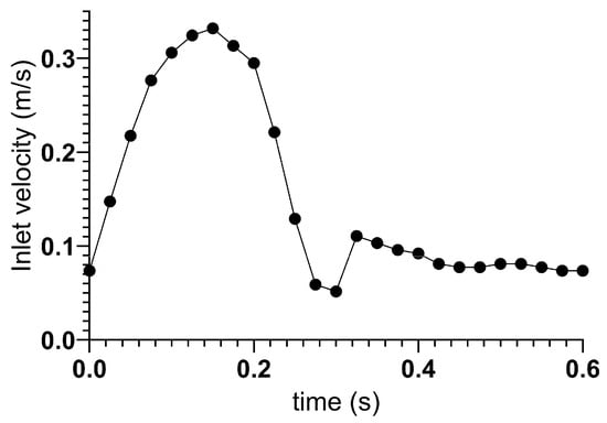
Figure 1.
The velocity curve used as the aorta inlet boundary condition.
The blood flow was modelled as incompressible and governed by the Reynolds-Averaged Navier–Stokes (RANS) equations. Conservation of mass was enforced through the continuity equation, while momentum conservation followed the Navier–Stokes equations in which the stress tensor included both molecular and turbulent viscosity. Turbulence was modelled using the realisable k-ε model, which solves additional transport equations for the turbulent kinetic energy (k) and its dissipation rate (ε) [38,39]. The model relates turbulent viscosity to k and ε, with coefficients that adapt dynamically to the local strain rate. This improves stability and predictive accuracy compared to the standard k-ε model, especially in flows with strong curvature and separation.
Different numerical solvers were applied depending on the platform. In COMSOL Multiphysics, the generalised-α time-stepping scheme was employed with second-order accuracy, and the linear systems were solved using the Generalised Minimum Residual (GMRES) iterative method. In Ansys Fluent, a second-order implicit time integration method was used together with the coupled pressure–velocity scheme. Ansys Discovery employed a GPU-accelerated lattice-Boltzmann-based solver, which enables rapid voxel-based flow computations but at reduced fidelity compared with finite element or finite volume approaches.
This combination allowed for benchmarking across platforms: Fluent provided the reference solution with high accuracy, COMSOL offered flexible finite element formulations in both 2D and 3D, and Discovery enabled accelerated prototyping.
For both 2D and 3D COMSOL simulations, the discretisation of fluids was increased to the second order to facilitate convergence.
In the 2D model, an unstructured tetrahedral mesh was generated with element sizes ranging from 0.063 mm to 2.23 mm, a maximum growth rate of 1.2, and a curvature factor of 0.3. Edge refinement was applied along the walls and boundaries, with element sizes between 0.00955 mm and 0.828 mm, while corner refinement enforced a minimum angle of 240° between boundaries to maintain the smoothness of curved walls. Five inflation layers were added at the walls with a stretching factor of 1.2. The resulting finite element mesh contained 6288 elements.
For the 3D model, an unstructured tetrahedral mesh was also used, with element sizes ranging from 0.137 mm to 1.27 mm, a maximum growth rate of 1.2, and a curvature factor of 0.3. Face refinement was applied to boundaries and walls, with element sizes between 0.00488 mm and 1.27 mm at the boundaries, and between 0.00685 mm and 0.446 mm at the walls. Corner refinement again enforced a minimum angle of 240° between surfaces, ensuring smooth curvature representation. Five boundary layers were applied with a stretching factor of 1.2. The final mesh consisted of 2,228,651 elements, which is approximately 354 times larger than the 2D case. Figure 2 shows the dimensioned 3D and 2D models and the 3D and 2D meshes on panels (a), (b), (c), and (d), respectively.
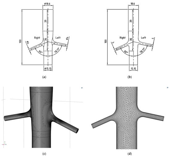
Figure 2.
Three- (a) and two-dimensional (b) models based on angiography measurements and three- (c) and two-dimensional (d) meshes in COMSOL Multiphysics.
2.3. Grid Study
For both 2D and 3D meshes, a mesh refinement study was performed following the Richardson extrapolation and Grid Convergence Index (GCI) methodology recommended by ASME. Three systematically refined meshes (M1–M3) with a refinement ratio r = 1.4 were employed. The quantity of interest was the peak velocity magnitude at the renal outlet.
The observed order of convergence p was computed as follows:
where , , and denote the velocity values obtained on the coarse, medium, and fine meshes, respectively.
The Richardson extrapolated value was estimated as follows:
The relative difference between the fine and medium meshes was calculated as follows:
Finally, the Grid Convergence Index between the fine and medium meshes was evaluated as follows:
with a safety factor of = 1.25.
A mesh refinement study was carried out for both 2D and 3D simulations. In 2D, the observed order of convergence was p = 3.09, while in 3D it was p = 3.17, both consistent with the theoretical expectation for quadratic elements. Richardson extrapolation gave values of = (2D) and = 0.4221 (3D). The fine-to-medium mesh differences were small—0.364% and 0.076%, respectively—with corresponding GCI values of 0.25% and 0.049%. These results confirm that both the 2D and 3D models are sufficiently refined, and the peak velocity magnitudes can be considered mesh independent.
In our previous study, volume flow rate, velocity magnitude, turbulent kinetic energy, and total pressure were measured. The primary focus of this study is not the flow characteristics of the renal artery, but the differences and similarities of the calculation methods; thus, they are demonstrated through only velocity curves to keep the paper concise.
2.4. Deep Neural Network Training in PyTorch
Surrogate modelling with deep neural networks (DNNs) was introduced to overcome the computational difficulties of repeated CFD evaluations. Four sets of design of experiment (DOE) data were produced with an increasing number of parameter combinations in order to evaluate the data requirements of the deep neural network (DNN) functions. The DOE tables consist of 1300, 2925, 6500, 13,975, and 83,075 lines. The calculation times are measured and extrapolated for 3D. Thus, the cost of calculation for the DNN training can be evaluated.
As an aspect of comparison, a fully connected Deep Feedforward Neural Network (DFNN) [33] was used as a supervised learning technique with Rectified Linear Unit (ReLu) activation function. The DFNN was tuned to obtain reliable predictions while avoiding overfitting. One of them will be shown below.
Depending on the dataset, training was carried out to determine the most accurate values of optimal pressure, flow velocity, and turbulent kinetic energy on the given interval of renal artery branching angles separately, meaning that simulations were performed for these target values uniquely and the DFNN was trained on these unique datasets one by one, so the output layer consists of 1 neuron.
To create the DFNN, the PyTorch 2.8. package of Python 3 was applied, which is often used to define neural networks. Based on the simulations, the input layer had 5 nodes as follows: left-side renal artery angulation (Ang_L [°]); right-side renal artery angulation (Ang_R [°]); systolic blood pressure (Sys [mmHg]); diastolic blood pressure (Dia [mmHg]); and time (t [s]), which was normalised by Min–Max scaling in the preprocessing phase. The dataset was segmented into training 80% and testing 20% subsets, and 10% of the training set was determined as validation data.
The model was trained with a batch size of 64 and a 0.001 training rate. To reduce the training time, an early stop criterion was also tested, which seemed at first sight an advantageous expansion of the network but worked well only on a few of the datasets, so in the final form, it was removed from the code. As an optimiser, the generally used Adaptive Moment Estimation (Adam) optimiser was chosen, while the Loss function was defined as Mean Squared Error (MSE).
During tuning, more structures of DFNN were tested to find the one that best fits the evaluations. The modifications were tested on the number of used neurons, the number of hidden layers, the dropout rate, and the learning rate. These results were evaluated based on the average value of the Coefficient of Determination, and the lowest value of resulted from a dataset that contains the results of simulating the velocity in the artery. The average of was calculated based on the groups inside the dataset. Based on the renal artery branching angles (Ang_L [°] column of the dataset), it was possible to create groups that represent one cardiac cycle at the given angle. These grouped values from simulation and prediction were compared to obtain the unique values for each group. Each model was trained through 100 epochs for equal comparison.
2.5. Deep Neural Network Training in COMSOL Multiphysics
COMSOL Multiphysics 6.3 has a built-in DNN training feature, which was used to train the models based on the design of experiment (DOE) data produced by simulation series. For each output parameter, a different DOE table was created; thus, a separate DNN model was trained for each parameter. The structure of the models was the same as the previous method, with the same input and output nodes. In the DOE table, the quantities of interest were velocity magnitude, pressure, and turbulent kinetic energy for both left- and right-side renal artery outlets, giving a total of 6 quantities of interest. The input parameters were the same as in the previous method: branching angles of the left and right renal arteries; the systolic and diastolic blood pressures; and time, which was determined by time steps taken by the solver.
Just like in the previous method, 10% of the training set was determined as validation data. The model was trained with a batch size of 128 and a 0.001 training rate. In COMSOL, lower batch size seriously slowed the calculation and produced higher losses. The default 512 batch size gave very high fluctuations in the loss rates, so the 128 batch size was selected as it seemed to be an optimal value. The optimiser (ADAM) and Loss function (MSE) were also the same. The structure of the networks was 5-256-128-64-64-1, based on the results of the previous method. The most important difference between the methods was the epoch count. While the PyTorch method was functional with only 200 epochs, in COMSOL, 5000 epochs were required. This difference affects the calculation times, as shown in the results.
3. Results
The Fluent simulations yielded a range of optimal branching angles for the renal artery, consistently aligning with previous findings while providing new insights into dynamic factors. It was noted that the new method produces results similar to prior approaches; however, it captures additional dynamic effects that may influence outcomes in cases of suboptimal angle branches.
3.1. Simulation Results in ANSYS Discovery
The simulations performed with Ansys 2024 R2 Discovery software took significantly less time than those performed with Ansys Fluent. Ansys Fluent works with a fine tetrahedral mesh and uses a turbulence model, and we ran a transient simulation. The running time per simulation was approximately 1.5 h, with a minimum preparation time of 30 min. Ansys Discovery applies voxel-based calculations, and transient simulations cannot be run, nor can turbulence models be applied. Thus, dynamic effects cannot be evaluated. Figure 3 shows the presumed laminar flow in the inspected area; streamlines are coloured based on velocity in Ansys Discovery software.
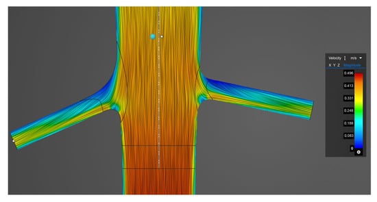
Figure 3.
Streamlines coloured based on velocity in the vicinity of the renal artery branching in Ansys Discovery software.
The benefit of using Ansys Discovery was that the simulation runtime was only around 1 min, preparation was minimal, the model was parametric, the branching angle could be specified as a variable, and thus the entire simulation series could be run at once.
The pressure and velocity values are shown as a function of the branching angle in Figure 4. The figure compares the results of the Ansys Fluent and Ansys Discovery software.
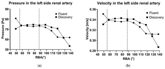
Figure 4.
Maximum pressure (a) and flow velocity (b) in the factor of the renal artery branching angle in Ansys 2020 R2 Fluent and Ansys 2024 R2 Discovery software.
In both methods, the optimal angle range can be observed, the boundaries of which are marked with an orange dotted line. However, at small branch angles, the two pieces of software gave contradictory results, which can be explained by dynamic effects that Discovery does not take into account.
3.2. Simulation Results in COMSOL Multiphysics
In COMSOL, to extrapolate 2D calculation times to 3D accurately, a single 3D simulation was performed. The calculation took 18.995 h to complete. A 2D simulation with the same parameters, but without parametric sweep or surrogate training, was performed, and the calculation time was found to be 0.118 h. This is a marked difference; the ratio between them is 160.9. This difference is a lot higher than previously speculated, so the or formula should not be used. Instead, we use the ratio to estimate 3D calculation times. The calculation times of the simulations performed in COMSOL are shown in Table 1.

Table 1.
Measured and estimated calculation times of COMSOL Multiphysics simulations.
The results of the 2D calculations show some inaccuracy, as predicted. In Figure 5, it is shown in both panels that the velocity values are lower than expected. In panel (a), the velocity values are presented during a heart cycle. The COMSOL 2D results are similar in the systolic phase but markedly different in the diastolic phase. In panel (b), the maximum velocity values are presented as a factor of the renal artery angulation. The lower velocities given by COMSOL 2D simulations can be seen, but the curve has similar characteristics to the curve produced by Fluent.
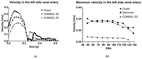
Figure 5.
Pressure (a) and flow velocity (b) in the factor of the renal artery branching angle in Fluent and Discovery software.
The results given by the 3D calculation in COMSOL are also different, even though the settings are identical, and the same 3D model was imported. In Figure 5, panel (a), the velocity results are higher than the Fluent results.
3.3. Deep Neural Network Training Results in PyTorch
To assess the results of the DNN training R2, the coefficient of determination is frequently used [40,41]. The values to compare simulation and prediction are presented in Table 2.
Table 2.
results of different DFNN structures with changing dropout rates through 100 epochs.
As a comparison, some tests were carried out on the vL dataset with a 0.003 training rate, but the training went chaotic, as shown in Figure 6, panel (b). Thus, the training rate was kept at 0.001.
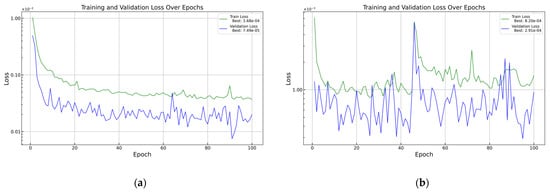
Figure 6.
Training curves for vL with different training rates: (a) 0.001 training rate and (b) 0.003 training rate.
These investigations show that if we want to train the model with these datasets, the most usable versions, depending on the dropout rate, are the 128-64-32-16 setup for 0 dropout, the 128-64-32-32 setup for 0.1 dropout, and the 256-128-64-64 setup for 0.2 dropout. The optimal structure for a 0.1 dropout rate could be chosen as 256-128-64-32, but it has produced wider . The results showed that a lower dropout rate may provide higher training success, but it must be mentioned that leaving the dropout rate out of the DFNN, overfitting can appear with higher probability. To prevent the system from co-adapting too much, it is necessary to use a dropout rate [42,43], which was chosen as 0.2 in our case because higher rates showed underfitting instead of overfitting during the tuning. The network was tested for higher dropout rates in some cases, but these results were not included in the table. The training success will be presented in Table 3 as a comparison. As a visualisation in Figure 7, velocity losses during the 200 epochs will be presented.
Table 3.
Performance of 256-128-64-64 setup with 0.2 dropout rate, 0.001 learning rate, and 200 epochs, trained in PyTorch.
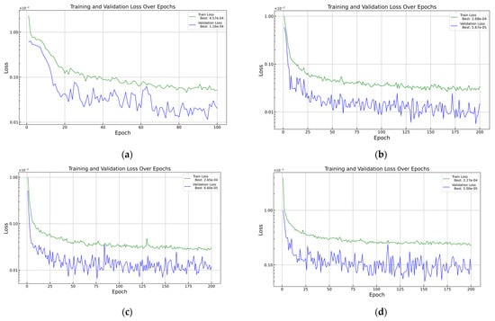
Figure 7.
Loss function in PyTorch using (a) 1 300, (b) 2 925, (c) 6 500, and (d) 13 975 samples.
In Table 3, two contradictions are visible. For the pressure predictions, the loss values are relatively high compared to the other values and the expert’s opinion. Despite these losses, the values are near 1, which means the model works well and is reliable. Compared to this, the losses for kinetic energy are enormously low, but the reliability of the model is widely scattered. The conclusion is possibly that the training samples are not enough for proper predictions. By increasing the number of samples, the pressure and velocity predictions did not change significantly, but the predictions for kinetic energy became better. Based on this, the outcomes for the later tests with higher training sample numbers were expected to be better. Because the 6500-sample case seems similar in reliability to the 13,975-sample case, but requires fewer sources, the velocity, pressure, and kinetic energy predictions are shown for visualisation and for a better overview at the same angle.
In Figure 8 panel (a), the velocity predictions for the left side renal artery can be seen in comparison with the original curve. These are relatively accurate, as the model was tuned on the velocity datasets. In panel (b), the predicted and original turbulent kinetic energy values are presented.
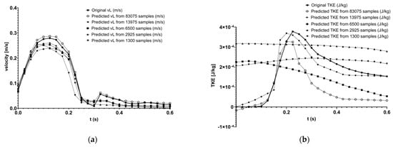
Figure 8.
Original and predicted velocity (a), and TKE (b) curve comparison in PyTorch using different sample counts.
3.4. Deep Neural Network Training Results in COMSOL Multiphysics
The COMSOL DNN training results are presented in Table 4. Increasing the sample count decreases losses only minimally, and interestingly, for the highest sample count, the losses are higher than for the previous two models. The R2 values, however, show a marked change; the values get closer to 1 at higher sample counts.
Table 4.
Training results of COMSOL DNN models with different sample sizes, 128 batch size, 0.001 learning rate, and 5000 epochs.
The COMSOL Loss functions are presented in Figure 9. The loss curves have high fluctuation; however, this seems higher than it really is because of the log scale on the y-axis. It is apparent that the more samples are used, the higher the fluctuation is, thanks to the same absolute batch size and thus decreasing batch–sample ratio.
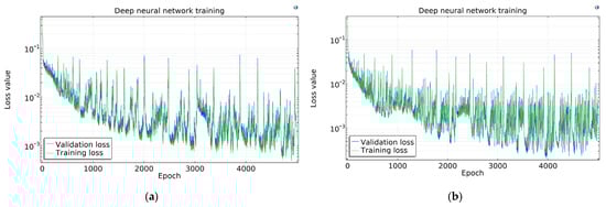
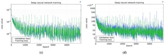
Figure 9.
Loss function in COMSOL using (a) 1300, (b) 2925, (c) 6500, and (d) 13,975 samples.
Figure 10 shows the original and predicted velocity, and TKE curves in COMSOL for each sample size in panels (a) and (b), respectively. It is apparent that on the velocity diagram, the 1300 sample curve does not follow the original curve adequately; the 2925 sample curve is much closer, the one produced using 6500 is even better, but the 13,975-sample curve does not become any better. The TKE values, however, show a very low similarity to the original curve even for 13,975 samples.
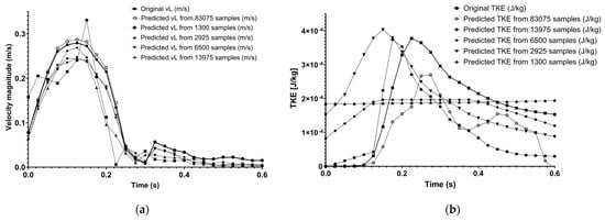
Figure 10.
Original and predicted velocity (a), and TKE (b) curve comparison in COMSOL using different sample counts.
4. Discussion
This study presents a comparative analysis of various computational approaches for simulating haemodynamics in the renal arteries, focusing on balancing simulation accuracy and computational cost. Three main computational fluid dynamics (CFD) frameworks—ANSYS Fluent, COMSOL Multiphysics (2D and 3D), and ANSYS Discovery—along with data-driven deep neural network (DNN) surrogate models, were investigated.
Among the physics-based simulations, ANSYS Fluent yielded results most consistent with those found in the literature [44], particularly during the systolic phase of the cardiac cycle. Despite lower absolute velocity values—which may be attributed to inlet conditions or inherent differences in solver settings—Fluent’s high fidelity supports its validity in assessing the haemodynamic effects of renal artery geometry. Thus, in this study, the Fluent results are used as the baseline, as they were previously published and shown to be sufficiently accurate and consistent with measured data [44].
Comparatively, COMSOL’s 2D model demonstrated reasonable agreement during the systolic phase, although inaccuracy was observed in the diastolic phase. This discrepancy is tolerable given the diastolic phase’s reduced significance in assessing peak flow phenomena.
As seen in Figure 5, panel (a), the COMSOL 3D model revealed unexpectedly higher velocity predictions than Fluent despite identical geometries and settings, likely originating from mesh density differences or solver-specific turbulence modelling. Importantly, computational costs in 3D were dramatically higher, with runtimes exceeding those in 2D by a factor of over 160. This finding underscores the critical importance of model dimensionality in simulation planning.
To address high computational demands, surrogate models using DNNs were implemented. With adequate training (≥6500 samples), DNNs predicted velocity and pressure with high R2 values (>0.98), providing rapid inference at negligible computational cost. Interestingly, turbulent kinetic energy (TKE) predictions showed low loss values but inconsistent reliability, indicating that larger datasets or more tailored network architectures might be required.
It is important to note that the inaccuracy of FEA or DNN models is within the measurement inaccuracy limits. For example, ultrasonic Doppler measurements [45] produce rather fuzzy diagrams than a precise curve, and even MR measurements have some deviation [46].
The results suggest that 6500 samples represent a reasonable compromise, achieving similar reliability to 13,975-sample models while requiring less training time and fewer computational resources. Oddly, the losses increased when training an 83,075-sample model. In Figure 11, the time cost–quality relations are demonstrated. These results suggest that increasing sample count beyond 6500 does not obtain better results, and oddly, for the COMSOL DNN, the losses are even higher. The velocity losses are similar for COMSOL and PyTorch DNN, pressure is markedly better in the case of COMSOL DNN, and TKE is more precise in PyTorch DNN. In the aspect of the prediction curve fitting the original, PyTorch is assumed to be better, as most R2 values are close to 1 above a certain sample count, whereas COMSOL R2 values are around 1 for only velocity diagrams.
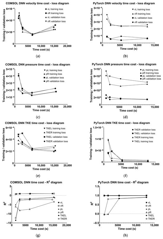
Figure 11.
Time cost–loss diagrams in COMSOL for (a) velocity, (c) pressure, and (e) turbulent kinetic energy; time cost–loss diagrams in PyTorch for (b) velocity, (d) pressure, and (f) turbulent kinetic energy, and time cost–R2 diagrams in (g) COMSOL and (h) in PyTorch.
In addition to velocity, turbulent kinetic energy (TKE) was also compared between CFD and DNN predictions. The results indicate that while the DNN initially struggled to reproduce TKE with limited training data, its accuracy improved as the dataset size increased. This behaviour is consistent with the higher complexity of turbulent flow fields, which typically require larger datasets to capture small-scale variations.
The inclusion of TKE highlights both the potential and the current limitations of surrogate modelling: whereas velocity can be predicted accurately even with smaller training sets, more data are required to obtain robust predictions for turbulence-related quantities. The other solution for accurate turbulence prediction would be to use physics informed DNN models, just like Wang et al. and Raissi et al. did [5,6].
In extrapolated 3D simulations, where each sample requires magnitudes more time, this reduction translates to significant savings. Accordingly, surrogate models become particularly valuable when exploring extensive parameter spaces, enabling surgical planning, real-time assessment, or app-based predictive tools using COMSOL App Builder.
An important question is posed: after how many simulations does training a neural network-based surrogate model become more cost-effective than performing additional FEA analyses? The total simulation + train time for the 6500 sample DNN model for all six parameters was 32,085 s for PyTorch and 39,560 s for COMSOL. If we compare these results to 3D simulation, which took 68,383 s for a single case, the cost effectiveness is obvious. But, for the 2D simulation, the cost-effectiveness calculation makes more sense. A single case simulation took 425 s without the preparation times. If we only calculate the computation time, the DNNs become cost-effective after 93 for COMSOL and 76 for PyTorch. So, these models are worth using if at least that amount of surgical planning is to be expected, for example. However, it is important to note that preparation times add up to the single case times, so these ratios are probably less in reality.
5. Conclusions
In conclusion, while high-fidelity simulations like those in Fluent remain indispensable for baseline validation, 2D simplifications and machine learning approaches offer robust, efficient alternatives. The findings offer a transferable methodology for other vascular regions (e.g., coronary arteries, cerebral vessels, or aneurysm studies), providing a powerful foundation for diagnostic, therapeutic, and planning applications. Future work should focus on refining surrogate model generalizability and incorporating more physiological variables, enabling even broader clinical and engineering integration. Short-term goals include optimising simulation and mathematical methods, refining previous findings, and assessing previously unexamined factors. The tangible outcome would be the establishment of an operational rule base that could immediately enable predictions related to the haemodynamic and physiological characteristics of the renal artery geometry without requiring further simulations. Long-term goals encompass developing additional rule bases applicable in various fields, thereby opening new avenues for diagnostics and surgical planning.
Author Contributions
Conceptualisation, D.C.; methodology, D.C. and A.K.; software, D.C., A.K., and Á.F.; validation, D.C.; formal analysis, D.C. and A.K.; investigation, D.C. and A.K.; resources, Á.F. and G.V.; data curation, D.C. and A.K.; writing—original draft preparation, D.C., T.S., and A.K.; writing—review and editing, D.C. and G.V.; visualisation, D.C. and A.K.; supervision, G.V., project administration, D.C. and G.V.; funding acquisition, D.C. and G.V. All authors have read and agreed to the published version of the manuscript.
Funding
This research was funded by the National Research, Development and Innovation Office, Hungary, under the University Research Scholarship Programme 2024-2.1.1-EKÖP. The APC was funded by the Faculty of Engineering at the University of Pécs, Hungary, within the framework of the ‘Call for Grant for Publication (3.0)’.
Data Availability Statement
The raw data supporting the conclusions of this article will be made available by the authors upon request.
Acknowledgments
The authors express their gratitude to their colleagues at the Department of Mechanical Engineering, FEIT, University of Pécs, for their support and encouragement. The authors acknowledge the support from SciEngineer regarding COMSOL. Special thanks to Balázs Szentei and the IT group of FEIT, University of Pécs, for the help in software acquisition.
Conflicts of Interest
Author Árpád Forberger was employed by the company SciEngineer. The remaining authors declare that the research was conducted in the absence of any commercial or financial relationships that could be construed as a potential conflict of interest.
References
- Kóczy, L.T. Symmetry or Asymmetry? Complex Problems and Solutions by Computational Intelligence and Soft Computing. Symmetry 2022, 14, 1839. [Google Scholar] [CrossRef]
- Kóczy, L.T. Fuzziness and Computational Intelligence: Dealing with Complexity and Accuracy. Soft Comput. 2006, 10, 178–184. [Google Scholar] [CrossRef]
- Kóczy, L.T.; Botzheim, J.; Gedeon, T.D. Fuzzy Models and Interpolation. In Forging New Frontiers: Fuzzy Pioneers I. Studies in Fuzziness and Soft Computing; Nikravesh, M., Kacprzyk, J., Zadeh, L.A., Eds.; Springer: Berlin/Heidelberg, Germany, 2007; Volume 217. [Google Scholar] [CrossRef]
- Kóczy, L.T.; Földesi, P.; Tüű-Szabó, B. Enhanced Discrete Bacterial Memetic Evolutionary Algorithm—An Efficacious Metaheuristic for the Traveling Salesman Optimization. Inf. Sci. 2018, 460–461, 389–400. [Google Scholar] [CrossRef]
- Duraisamy, K.; Iaccarino, G.; Xiao, H. Annual Review of Fluid Mechanics Turbulence Modeling in the Age of Data. Annu. Rev. Fluid Mech. 2019, 51, 357–377. [Google Scholar] [CrossRef]
- Raissi, M.; Yazdani, A.; Karniadakis, G.E. Hidden Fluid Mechanics: A Navier-Stokes Informed Deep Learning Framework for Assimilating Flow Visualization Data. arXiv 2018, arXiv:1808.04327. [Google Scholar] [CrossRef]
- Mugdha, S.B.S.; Uddin, M.; Das, H. A Comprehensive Approach to Heart Disease Analysis Using Machine Learning Algorithms. Int. J. Autom. Smart Technol. 2024, 14, 1–11. [Google Scholar] [CrossRef]
- Csonka, D.; Kalmár Nagy, K.; Szakály, P.; Szukits, S.; Bogner, P.; Koller, A.; Kun, S.; Wittmann, I.; Háber, I.E.; Horváth, I.G. Optimal Renal Artery-Aorta Angulation Revealed by Flow Simulation. Kidney Blood Press Res. 2023, 48, 249–259. [Google Scholar] [CrossRef]
- Kwak, B.R.; Bäck, M.; Bochaton-Piallat, M.L.; Caligiuri, G.; Daemen, M.J.A.P.; Davies, P.F.; Hoefer, I.E.; Holvoet, P.; Jo, H.; Krams, R.; et al. Biomechanical Factors in Atherosclerosis: Mechanisms and Clinical Implications. Eur. Heart J. 2014, 35, 3013–3020. [Google Scholar] [CrossRef]
- Schoenberg, S.O.; Bock, M.; Kallinowski, F.; Just, A. Correlation of Hemodynamic Impact and Morphologic Degree of Renal Artery Stenosis in a Canine Model. J. Am. Soc. Nephrol. 2000, 11, 2190–2198. [Google Scholar] [CrossRef]
- Sabbah, H.N.; Hawkins, E.T.; Stein, P.D. Flow Separation in the Renal Arteries. Arteriosclerosis 1984, 4, 28–33. [Google Scholar] [CrossRef]
- Murray, C.D. The Physiological Principle of Minimum Work Applied to the Angle of Branching of Arteries. J. Gen. Physiol. 1926, 9, 835–841. [Google Scholar] [CrossRef]
- Huo, Y.; Finet, G.; Lefevre, T.; Louvard, Y.; Moussa, I.; Kassab, G.S. Which Diameter and Angle Rule Provides Optimal Flow Patterns in a Coronary Bifurcation? J. Biomech. 2012, 45, 1273–1279. [Google Scholar] [CrossRef]
- ANZAI, Y.; TAGAWA, T.; SHIBATA, H. Numerical Simulation of Solid-Gas-Liquid Multiphase Flow on GPU. Int. J. Microgravity Sci. Appl. 2022, 39, 390102. [Google Scholar] [CrossRef]
- Brunton, S.L.; Noack, B.R.; Koumoutsakos, P. Annual Review of Fluid Mechanics Machine Learning for Fluid Mechanics. Annu. Rev. Fluid Mech. 2019, 52, 477–508. [Google Scholar] [CrossRef]
- Bishop, C.M. Pattern Recognition and Machine Learning; Jordan, M., Kleinberg, J., Schölkopf, B., Eds.; Springer: Berlin/Heidelberg, Germany, 2006; Volume 4, p. 738. [Google Scholar] [CrossRef]
- Rygiel, P.; Suk, J.; Yeung, K.K.; Brune, C.; Wolterink, J.M. Active Learning for Deep Learning-Based Hemodynamic Parameter Estimation. arXiv 2025, arXiv:2503.03453. [Google Scholar] [CrossRef]
- Jnini, A.; Goordoyal, H.; Dave, S.; Vella, F.; Fraser, K.H.; Korobenko, A. Physics-Constrained DeepONet for Surrogate CFD Models: A Curved Backward-Facing Step Case. arXiv 2025, arXiv:2503.11196. [Google Scholar]
- Wang, H.; Cao, Y.; Huang, Z.; Liu, Y.; Hu, P.; Luo, X.; Song, Z.; Zhao, W.; Liu, J.; Sun, J.; et al. Recent Advances on Machine Learning for Computational Fluid Dynamics: A Survey. arXiv 2024, arXiv:2408.12171. [Google Scholar] [CrossRef]
- Roznowicz, D.; Stabile, G.; Demo, N.; Fransos, D.; Rozza, G. Large-Scale Graph-Machine-Learning Surrogate Models for 3D-Flowfield Prediction in External Aerodynamics. Adv. Model. Simul. Eng. Sci. 2024, 11, 6. [Google Scholar] [CrossRef]
- Venier, C.; Urrutia, R.; Yao, J.; Ghasem, N. Combining CFD and AI/ML Modeling to Improve the Performance of Polypropylene Fluidized Bed Reactors. Fluids 2024, 9, 298. [Google Scholar] [CrossRef]
- Wang, J.; Wu, J.; Xiao, H. A Physics-Informed Machine Learning Approach of Improving RANS Predicted Reynolds Stresses. In Proceedings of the 55th AIAA Aerospace Sciences Meeting, Grapevine, TX, USA, 9–13 January 2017. [Google Scholar] [CrossRef]
- Hastie, T.; Tibshirani, R.; Friedman, J. The Elements of Statistical Learning; Springer Science & Business Media: New York, NY, USA, 2009. [Google Scholar] [CrossRef]
- Draper, N.R.; Smith, H. Applied Regression Analysis; Wiley: Hoboken, NJ, USA, 1998; pp. 1–716. [Google Scholar] [CrossRef]
- Montgomery, D.C.; Peck, E.A.; Vining, G.G. Introducing To Linear Regression Analysis, 5th ed.; John Wiley & Sons: Hoboken, NJ, USA, 2012; p. 642. [Google Scholar]
- Breiman, L.; Friedman, J.H.; Olshen, R.A.; Stone, C.J. Classification and Regression Trees; Chapman and Hall: New York, NY, USA, 2017; pp. 1–358. [Google Scholar] [CrossRef]
- Friedman, J.H. Greedy Function Approximation: A Gradient Boosting Machine. Ann. Stat. 2001, 29, 1189–1232. [Google Scholar] [CrossRef]
- Salzberg, S.L. C4.5: Programs for Machine Learning by J. Ross Quinlan. Morgan Kaufmann Publishers, Inc., 1993. Mach. Learn. 1994, 16, 235–240. [Google Scholar] [CrossRef]
- Smola, A.J.; Schölkopf, B. A Tutorial on Support Vector Regression. Stat. Comput. 2004, 14, 199–222. [Google Scholar] [CrossRef]
- Vapnik, V.N. The Nature of Statistical Learning Theory; Springer: New York, NY, USA, 1995. [Google Scholar] [CrossRef]
- Chang, C.C.; Lin, C.J. LIBSVM: A Library for Support Vector Machines. ACM Trans. Intell. Syst. Technol. 2011, 2, 1–27. [Google Scholar] [CrossRef]
- Goodfellow, I.; Bengio, Y.; Courville, A. Deep Learning; MIT Press: Cambridge, MA, USA, 2016. [Google Scholar]
- Hornik, K.; Stinchcombe, M.; White, H. Multilayer Feedforward Networks Are Universal Approximators. Neural Netw. 1989, 2, 359–366. [Google Scholar] [CrossRef]
- O’Flynn, P.M.; O’Sullivan, G.; Pandit, A.S. Geometric Variability of the Abdominal Aorta and Its Major Peripheral Branches. Ann. Biomed. Eng. 2010, 38, 824–840. [Google Scholar] [CrossRef]
- Liu, H.; Lan, L.; Abrigo, J.; Ip, H.L.; Soo, Y.; Zheng, D.; Wong, K.S.; Wang, D.; Shi, L.; Leung, T.W.; et al. Comparison of Newtonian and Non-Newtonian Fluid Models in Blood Flow Simulation in Patients With Intracranial Arterial Stenosis. Front. Physiol. 2021, 12, 718540. [Google Scholar] [CrossRef]
- Xiang, J.; Tremmel, M.; Kolega, J.; Levy, E.I.; Natarajan, S.K.; Meng, H. Newtonian Viscosity Model Could Overestimate Wall Shear Stress in Intracranial Aneurysm Domes and Underestimate Rupture Risk. J. Neurointerv. Surg. 2012, 4, 351–357. [Google Scholar] [CrossRef]
- Javadzadegan, A.; Simmons, A.; Barber, T. Spiral Blood Flow in Aorta–Renal Bifurcation Models. Comput. Methods Biomech. Biomed. Eng. 2015, 19, 964–976. [Google Scholar] [CrossRef]
- Shih, T.H.; Liou, W.W.; Shabbir, A.; Yang, Z.; Zhu, J. A New K-ϵ Eddy Viscosity Model for High Reynolds Number Turbulent Flows. Comput. Fluids 1995, 24, 227–238. [Google Scholar] [CrossRef]
- Fluent Thoery Guide Ansys Fluent Theory Guide; ANSYS Inc.: Canonsburg, PA, USA, 2013; Volume 15317, pp. 724–746.
- Dzięcioł, J.; Sas, W. Perspective on the Application of Machine Learning Algorithms for Flow Parameter Estimation in Recycled Concrete Aggregate. Materials 2023, 16, 1500. [Google Scholar] [CrossRef]
- Varone, G.; Ieracitano, C.; Çiftçioğlu, A.Ö.; Hussain, T.; Gogate, M.; Dashtipour, K.; Al-Tamimi, B.N.; Almoamari, H.; Akkurt, I.; Hussain, A. A Novel Hierarchical Extreme Machine-Learning-Based Approach for Linear Attenuation Coefficient Forecasting. Entropy 2023, 25, 253. [Google Scholar] [CrossRef] [PubMed]
- Hinton, G.E.; Srivastava, N.; Krizhevsky, A.; Sutskever, I.; Salakhutdinov, R.R. Improving Neural Networks by Preventing Co-Adaptation of Feature Detectors. arXiv 2012, arXiv:1207.0580. [Google Scholar] [CrossRef]
- Srivastava, N.; Hinton, G.; Krizhevsky, A.; Sutskever, I.; Salakhutdinov, R. Dropout: A Simple Way to Prevent Neural Networks from Overfitting. J. Mach. Learn. Res. 2014, 15, 1929–1958. [Google Scholar]
- Maier, S.E.; Scheidegger, M.B.; Liu, K.; Schneider, E.; Bellinger, A.; Boesiger, P. Renal Artery Velocity Mapping with MR Imaging. J. Magn. Reson. Imaging 1995, 5, 669–676. [Google Scholar] [CrossRef]
- Yamamoto, T.; Ogasawara, Y.; Kimura, A.; Tanaka, H.; Hiramatsu, O.; Tsujioka, K.; Lever, M.J.; Parker, K.H.; Jones, C.J.H.; Caro, C.G.; et al. Blood Velocity Profiles in the Human Renal Artery by Doppler Ultrasound and Their Relationship to Atherosclerosis. Arter. Thromb. Vasc. Biol. 1996, 16, 172–177. [Google Scholar] [CrossRef]
- Keegan, J.; Patel, H.C.; Simpson, R.M.; Mohiaddin, R.H.; Firmin, D.N. Inter-Study Reproducibility of Interleaved Spiral Phase Velocity Mapping of Renal Artery Haemodynamics. J. Cardiovasc. Magn. Reson. 2015, 17, 8. [Google Scholar] [CrossRef]
Disclaimer/Publisher’s Note: The statements, opinions and data contained in all publications are solely those of the individual author(s) and contributor(s) and not of MDPI and/or the editor(s). MDPI and/or the editor(s) disclaim responsibility for any injury to people or property resulting from any ideas, methods, instructions or products referred to in the content. |
© 2025 by the authors. Licensee MDPI, Basel, Switzerland. This article is an open access article distributed under the terms and conditions of the Creative Commons Attribution (CC BY) license (https://creativecommons.org/licenses/by/4.0/).