EP-REx: Evidence-Preserving Receptive-Field Expansion for Efficient Crack Segmentation

Abstract

Crack segmentation plays a vital role in ensuring structural safety, yet practical deployment on resource-limited platforms demands models that balance accuracy with efficiency. While high-accuracy models often rely on computationally heavy designs to expand their receptive fields, recent lightweight approaches typically delay this expansion to the deepest, low-resolution layers to maintain efficiency. This design choice leaves long-range context underutilized, where fine-grained evidence is most intact. In this paper, we propose an evidence-preserving receptive-field expansion network, which integrates a multi-scale dilated block to efficiently capture long-range context from the earliest stages and an input-guided gate that leverages grayscale conversion, average pooling, and gradient extraction to highlight crack evidence directly from raw inputs. Experiments on six benchmark datasets demonstrate that the proposed network achieves consistently higher accuracy under lightweight constraints. Each of the three proposed variants—Base, Small, and Tiny—outperforms its corresponding baselines with larger parameter counts, surpassing a total of 13 models. For example, the Base variant reduces parameters by 66% compared to the second-best CrackFormer II and floating-point operations by 53% on the Ceramic dataset, while still delivering superior accuracy. Pareto analyses further confirm that the proposed model establishes a superior accuracy–efficiency trade-off across parameters and floating-point operations.

1. Introduction

Crack segmentation is a core task for the automation of structural safety inspection and preventive maintenance in civil and architectural infrastructure [1]. Traditionally, such inspections are performed manually by human experts, a process that is often time-consuming, subjective, and hazardous [2]. Computer vision algorithms enable systematic and reproducible crack detection, reducing subjective variability in structural health monitoring [3]. Nevertheless, transitioning this technology from a controlled laboratory setting to practical, real-world applications introduces a critical trade-off between two conflicting goals [4]. On one hand, the safety-critical nature of inspection imposes stringent accuracy requirements [5]. On the other hand, for on-device processing on platforms such as drones or mobile robots, models should be extremely lightweight and computationally efficient [6]. These platforms operate under tight resource budgets, including limited battery life, memory, and processing power, which necessitates a design that minimizes computational cost while maintaining substantial accuracy to ensure swift, reliable, and continuous operation in the field [7]. Meeting these on-device constraints typically requires models with fewer than five million parameters and a computational cost of several hundred million floating-point operations (FLOPs) [8].

A central challenge in crack segmentation lies in acquiring sufficient global context, as the elongated and continuous nature of cracks requires a wide receptive field to distinguish them from background patterns and to preserve mask integrity [9]. Conventional approaches enlarge the receptive field by stacking convolutional layers. However, this strategy is computationally expensive and unsuitable for compact models. To satisfy efficiency requirements, recent lightweight crack segmentation models adopt depthwise or group convolutions, channel reduction, and slim encoder–decoder designs [10,11,12]. However, their strategy for receptive-field expansion is often limited, leaving long-range context underutilized in the early stages where fine-grained evidence is most intact. A typical example of this is confining dilated convolutions—an effective tool for receptive-field expansion—to the deepest, low-resolution layers to avoid computational cost and gridding artifacts at higher resolutions. This leads to a reliance on post-hoc refinements, such as attention or sharpening filters, to compensate for information that has already been lost, ultimately limiting accuracy under resource-constrained conditions.

In this work, we propose Evidence-Preserving Receptive-field Expansion network (EP-REx), a crack segmentation network designed to enlarge the receptive field efficiently under lightweight constraints. Conventional dilated convolutions provide a cost-effective way to extend context, but when applied with large dilation rates on high-resolution maps, they often introduce gridding artifacts and fail to capture fine details crucial for hairline cracks [13]. EP-REx addresses this limitation with a multi-scale dilated block (MSDB) of parallel dilated depthwise convolutions, where small dilation rates preserve local detail and larger rates capture broader context, collectively achieving a balanced receptive-field expansion at low cost. To further strengthen this process, EP-REx incorporates an input-guided gate (IG-Gate), which derives a parameter-free map from input intensity and gradient cues to modulate feature responses. This input-guided mechanism efficiently leverages raw-image cues to emphasize crack continuity, thereby complementing the dilated design and supporting more balanced receptive-field expansion. The main contributions of this work are summarized as follows:

• We propose EP-REx, a compact architecture that efficiently enlarges the receptive field to capture global context while simultaneously preserving the critical pixel-level evidence essential for crack segmentation, making it suitable for resource-constrained applications.
• We introduce a multi-scale block featuring parallel dilated depthwise convolutions. Our ablation studies validate that this design, which captures both broad context and fine details, is more effective than standard convolutional blocks for improving segmentation accuracy in a lightweight setting.
• We present IG-Gate, a parameter-free module that leverages raw input intensity and gradient cues to modulate feature responses. We demonstrate through ablation studies that this mechanism effectively enhances performance and works synergistically with our multi-scale block to better preserve critical pixel-level cues.

2. Related Work

A pivotal moment in neural network-based semantic segmentation was the introduction of fully convolutional network (FCN), one of the earliest widely adopted end-to-end frameworks for dense, pixel-wise prediction achieved by replacing final fully connected layers with convolutional ones [14]. This innovation allowed the network to process images of arbitrary sizes and produce a corresponding spatial map of predictions. Building upon this, the U-Net architecture introduced a symmetric encoder–decoder structure complemented by skip connections [15]. The encoder path progressively downsamples the input to capture high-level semantic context, while the decoder path gradually upsamples the feature maps to recover spatial resolution. Crucially, the skip connections bridge these two paths, allowing the decoder to reuse fine-grained feature maps from the encoder. This mechanism was shown to be highly effective for precise localization and has become a standard in different domains requiring the accurate delineation of fine-grained structures [16,17].

Subsequent works have further refined these foundational architectures. The DeepLab series, for instance, introduced atrous (dilated) convolutions and atrous spatial pyramid pooling (ASPP) to capture multi-scale context without sacrificing spatial resolution [18]. More recently, the paradigm has shifted towards transformer-based architectures, which excel at capturing long-range dependencies. SegFormer demonstrated that a hierarchical transformer encoder paired with a simple multi-layer perceptron decoder could achieve state-of-the-art performance efficiently [19]. The trend shifted towards hybrid models that combine the local feature extraction strengths of convolutional networks with the global context modeling of transformers, a popular strategy for improving segmentation accuracy in complex scenes [20,21,22].

While the accuracy of neural networks grew, their computational and memory demands often became prohibitive, creating a significant barrier to deployment on resource-constrained platforms such as mobile phones and embedded devices [23]. Specifically, traditional encoder–decoder architectures, such as FCN, often involve tens of millions of parameters and computational costs on the order of tens of giga FLOPs, as they rely heavily on standard convolutions, where every input channel is densely connected to every output channel [8,24]. This challenge spurred a dedicated research effort into creating efficient network designs that balance performance with computational cost [25]. A key innovation in this area was the use of depthwise separable convolutions, popularized by MobileNet [26]. This technique factorizes a standard convolution into two separate steps: a depthwise convolution that applies a single filter per input channel, followed by a pointwise convolution, which is a 1 × 1 convolution, to combine the outputs. This factorization drastically reduces the number of parameters and computations. ShuffleNet further optimized this concept by introducing pointwise group convolutions and a novel channel shuffle operation, which facilitates information flow between channel groups to maintain high accuracy while minimizing cost [24,27]. Beyond architectural innovations, model compression techniques have also become crucial. Methods including network pruning, which systematically identifies and removes unimportant weights or entire network connections post-training [28,29], and knowledge distillation, where a compact student model is trained to mimic the output of a larger, more powerful teacher model [30], have enabled the creation of highly efficient models without significant performance degradation.

This evolutionary trajectory has directly shaped the development of crack segmentation methods. Early efforts involved applying foundational architectures, such as FCNs [31,32] and U-Net [33], directly to the problem. These models supplanted traditional, often hand-engineered image processing methods [1,34] by demonstrating superior performance, robustness, and generalization across different surface types and imaging conditions. More recently, transformer-based modules have been employed to capture the long-range continuity of cracks [35]. Finally, the emphasis on lightweight and efficient architectures, exemplified by MobileNet and ShuffleNet [27], has motivated recent crack segmentation models such as RHACrackNet [10] and LMNet [36], which adapt these efficiency principles to enable real-time inspection in resource-constrained environments.

As the field matured, research focused on developing specialized architectures to address the unique challenges of crack detection, such as their fine-grained, elongated nature and the presence of complex background noise that can mimic crack-like features. To enhance feature representation, DeepCrack aggregated hierarchical features from all convolutional layers to create a richer, multi-scale understanding of the input [37], while others refined the information flow in skip connections using residual blocks and sharpening kernels to reduce the semantic gap between encoder and decoder features [9]. Attention mechanisms were widely adopted to help models focus on salient crack regions and suppress irrelevant background patterns [10,38]. More recently, transformers were integrated to capture the long-range dependencies inherent in crack structures. This began with hybrid models such as CrackFormer, which embedded self-attention modules into a convolutional framework [35], and evolved into powerful dual-encoder networks that combine the local feature extraction strengths of convolutional networks with the global context modeling of transformers [39,40,41].

Concurrently, the practical need for real-time, on-device inspection has intensified the focus on efficient design principles. Recent lightweight models often combine efficient backbones with specialized modules to maintain accuracy. For example, RHACrackNet [10] utilizes depthwise separable convolutions and residual connections for efficiency, while incorporating spatial and channel attention to preserve crack continuity. Similarly, CSNet [11] employs group convolutions with shuffling and also uses attention mechanisms, though it relies on DenseASPP for multi-scale processing, which can risk losing feature details at high dilation rates. More complex designs such as LMNet [36] use depthwise convolutions but add a suite of modules—including a trainable edge extractor and a feature-reconnection module—to explicitly compensate for information loss during downsampling and enhance feature representation. An active learning framework combining subset searching and weighted sampling was proposed to enhance efficiency and accuracy in crack detection [42]. A Faster R-CNN–based approach was developed to automatically identify and localize multiple seismic damage types in reinforced concrete columns from images [43].

A common drawback of conventional models is their limited ability to capture long-range context in the early stages, where fine-grained evidence is most intact. This limitation arises because, to avoid high computational costs and potential gridding artifacts, such models typically restrict large-rate dilated convolutions to their deepest, low-resolution layers [11,36]. As a result, they often rely on auxiliary modules, such as attention or feature-reconnection blocks, to compensate for this limited contextual view and to recover details lost during downsampling. This strategy was compensatory, since it fixed information loss only after it had already occurred. This motivated a different approach where a more efficient receptive field expansion is integrated directly into the feature extraction process from the outset.

3. Proposed Method

In this section, we present the proposed network for crack segmentation, designed to attain a favorable balance between segmentation accuracy and computational efficiency, as illustrated in Figure 1. We begin with the preliminaries, where we mathematically define the crack segmentation and outline the motivation of our architectural design. We then detail our solution, breaking it down into its key components: MSDB for feature extraction and a parameter-free IG-Gate for feature modulation.

3.1. Preliminaries

Let $\mathcal{X}={\mathbb{R}}^{H\times W\times 3}$ be the space of input RGB images and $\mathcal{Y}={\{0,1\}}^{H\times W}$ be the space of corresponding binary ground truth segmentation masks, where H and W denote the image height and width, respectively. For a given mask $M\in \mathcal{Y}$, a value of $M_{ij}=1$ at pixel coordinate $(i,j)$ indicates the presence of a crack, while $M_{ij}=0$ indicates the background. The objective of crack segmentation is to learn a function $\mathcal{F}:\mathcal{X}\to {[0,1]}^{H\times W}$ that approximates the true underlying mapping from an image $I\in \mathcal{X}$ to its mask $M\in \mathcal{Y}$. The function $\mathcal{F}$ is approximated by a neural network parameterized by a set of weights $\theta$. The network takes an image I as input and outputs a score map $P=\mathcal{F}(I;\theta )$, where each element $P_{ij}\in [0,1]$ represents the score that pixel $(i,j)$ belongs to a crack. The learning process aims to find the optimal parameters ${\theta }^{\ast }$ that minimize a chosen loss function $\mathcal{L}$ over a training dataset $\mathcal{D}={\left\{(I_n,M_n)\right\}}_{n=1}^N$, where N denotes the number of training samples as

$${\theta }^{\ast }=arg\underset{\theta }{min}{\displaystyle \frac{1}{N}}\sum _{n=1}^N\mathcal{L}(\mathcal{F}(I_n;\theta ),M_n).$$

(1)

In our study, the loss function $\mathcal{L}$ is defined as a hybrid Dice + CrossEntropy loss, formulated as

$$\mathcal{L}={\mathcal{L}}_{\mathrm{Dice}}+{\mathcal{L}}_{\mathrm{CE}},$$

(2)

where ${\mathcal{L}}_{\mathrm{CE}}$ is the standard pixel-wise cross-entropy loss and ${\mathcal{L}}_{\mathrm{Dice}}$ is the soft Dice loss that directly optimizes region overlap between the prediction P and ground truth M.

The effective approximation of the function $\mathcal{F}$ for crack segmentation requires addressing two competing demands. The first is the need for a global context, which involves capturing long-range spatial dependencies to maintain the continuity of elongated cracks. The second is the need to preserve local evidence, the fine-grained, pixel-level details such as subtle intensity changes that are crucial for detecting hairline cracks. Conventional methods for expanding the receptive field to capture global context, such as stacking a number of layers, can be computationally demanding for lightweight models. While efficient alternatives such as aggressive downsampling exist, they lead to a severe loss of spatial resolution, permanently destroying local evidence.

Dilated convolutions offer a more efficient way to enlarge the receptive field without downsampling. However, they introduce a new challenge as the sparse sampling problem. Using a single, large dilation rate on high-resolution feature maps can cause the sampling grid to miss the very fine-grained details that define hairline cracks, leading to fragmented predictions and gridding artifacts. These competing requirements create a fundamental dilemma, defining the core challenge as the need to efficiently expand the receptive field for global context without losing the local evidence necessary for precise detection. Our work is motivated by the need to resolve said context-evidence dilemma by leveraging the efficiency of dilated convolutions while mitigating their inherent drawbacks.

3.2. Proposed Architecture: Encoder Path

To address the problem defined above, we propose an encoder–decoder architecture, illustrated in Figure 1. The proposed model is specifically designed to tackle the conflicting requirements of context aggregation and evidence preservation through a dual-pronged strategy within its encoder. The encoder path consists of L stages. Let $X^{(l-1)}$ be the output feature map of the $(l-1)$-th stage. The operation at the l-th stage ($l=1,\dots ,L$) begins with feature extraction, where the input feature map is processed by a sequence of $N_b$ MSDBs. Let $X_{MSDB,0}^{\left(l\right)}=X^{(l-1)}$. Then, for $b=1,\dots ,N_b$, the features are sequentially refined as

$$X_{MSDB,b}^{\left(l\right)}={\mathcal{F}}_{MSDB,b}^{\left(l\right)}\left(X_{MSDB,b-1}^{\left(l\right)}\right),$$

(3)

where ${\mathcal{F}}_{MSDB,b}^{\left(l\right)}$ is the b-th MSDB in the stage. Let the final output of the MSDB sequence be $X_{MSDB}^{\left(l\right)}=X_{MSDB,N_b}^{\left(l\right)}$. Concurrently, IG-Gate generates a spatial attention score map, $G^{\left(l\right)}$, from the original input image I as

$$G^{\left(l\right)}={\mathcal{G}}_{IG}^{\left(l\right)}\left(I\right),$$

(4)

where ${\mathcal{G}}_{IG}^{\left(l\right)}$ denotes the function of IG-Gate at the l-th stage. The resulting score map modulates the extracted features via element-wise multiplication (⊙) as

$$X_{mod}^{\left(l\right)}=X_{MSDB}^{\left(l\right)}\odot G^{\left(l\right)}.$$

(5)

Finally, the modulated feature map is downsampled using a max-pooling operation, ${\mathcal{P}}_{max}(·)$, to produce the output for the current stage as

$$X^{\left(l\right)}={\mathcal{P}}_{max}\left(X_{mod}^{\left(l\right)}\right)$$

(6)

3.3. Multi-Scale Dilated Block (MSDB)

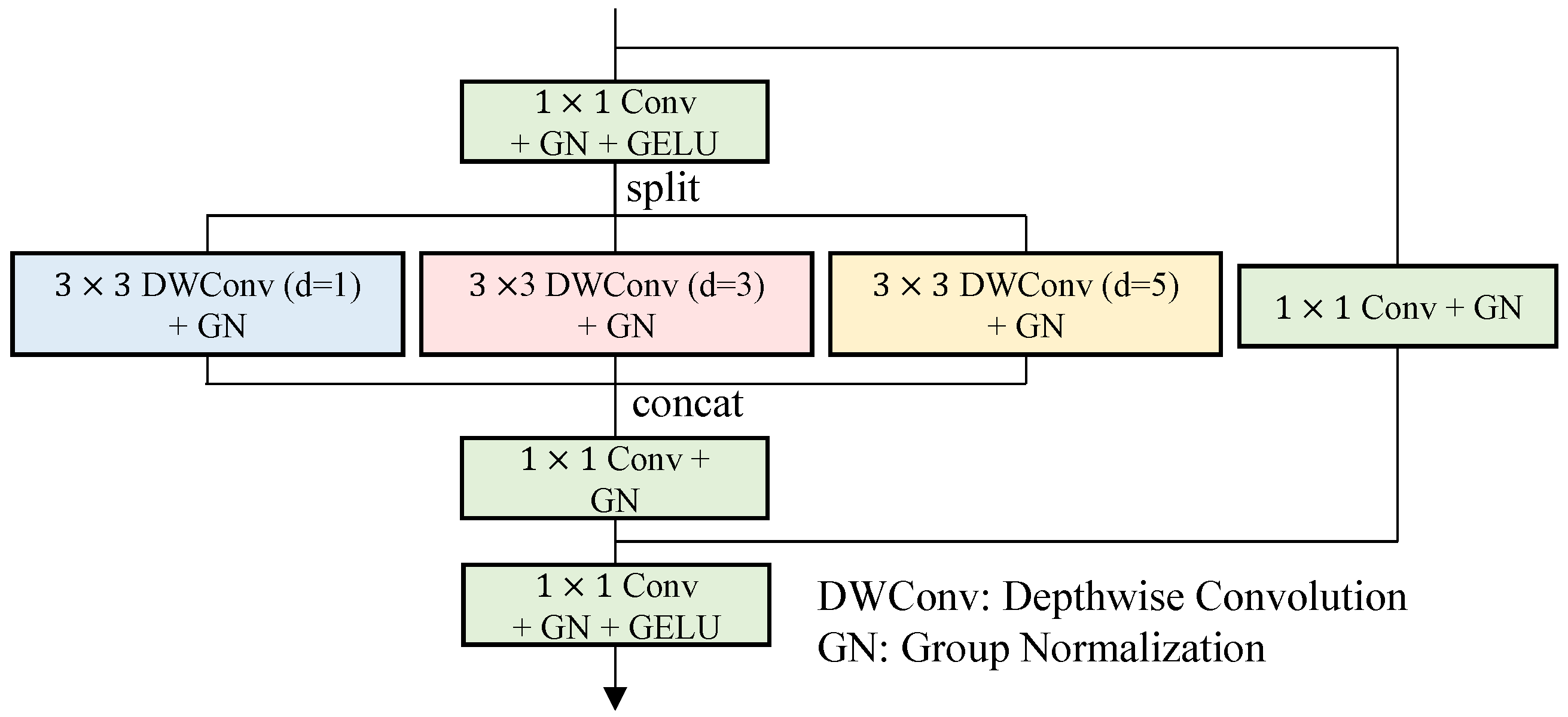
MSDB, depicted in Figure 2, is the core feature extractor in our encoder, designed to efficiently expand the receptive field.

MSDB achieves receptive field expansion by capturing multi-scale contextual information through parallel dilated convolutions, which mitigates the sparse sampling problem of using a single large dilation rate. Let the input to the block be a feature map $X_{in}\in {\mathbb{R}}^{H^{\prime }\times W^{\prime }\times C^{\prime }}$. First, a pointwise convolution (${\mathrm{Conv}}_{1\times 1}$) projects the input features, preparing them for multi-scale processing as

$$X_{proj}={\mathrm{Conv}}_{1\times 1,in}\left(X_{in}\right).$$

(7)

The projected feature map $X_{proj}$ is then fed into K parallel branches. In our implementation, $K=3$. Each branch $k\in \{1,\dots ,K\}$ applies a $3\times 3$ depthwise convolution with a different dilation rate $d_k$ as

$$X_k={\mathcal{F}}_{DW}^{d_k}\left(X_{proj}\right)\mathrm{for}k=1,2,3,$$

(8)

where the dilation rates are set to $d_1=1,d_2=3,d_3=5.$ The branch with a small dilation rate captures fine-grained local details, while branches with larger rates capture broader context. The feature maps from all branches are normalized, activated, and then concatenated along the channel dimension as

$$X_{cat}=[{\sigma }_{act}\left(\mathcal{N}\left(X_1\right)\right),{\sigma }_{act}\left(\mathcal{N}\left(X_2\right)\right),{\sigma }_{act}\left(\mathcal{N}\left(X_3\right)\right)].$$

(9)

Finally, another pointwise convolution (${\mathrm{Conv}}_{1\times 1,out}$) fuses the concatenated multi-scale features to produce $X_{fused}$ as

$$X_{fused}={\mathrm{Conv}}_{1\times 1,out}\left(X_{cat}\right).$$

(10)

To preserve the original information and stabilize training, a residual connection is applied. If the input and output channels differ, a $1\times 1$ projection is used to align dimensions as

$$X_{out}=X_{fused}+{\mathcal{P}}_{proj}\left(X_{in}\right),$$

(11)

where ${\mathcal{P}}_{proj}$ denotes either the identity mapping or a $1\times 1$ convolution for channel adjustment. While parallel dilated convolutions have been previously explored in generic semantic segmentation (e.g., DeepLabV3+ [18]), their use in crack segmentation has been rare and typically confined to the final encoder stage due to the sparse sampling issue. In contrast, we extend their application across all encoder stages and combine them with IG-Gate, enabling more effective receptive field expansion under lightweight constraints.

3.4. Input-Guided Gate (IG-Gate)

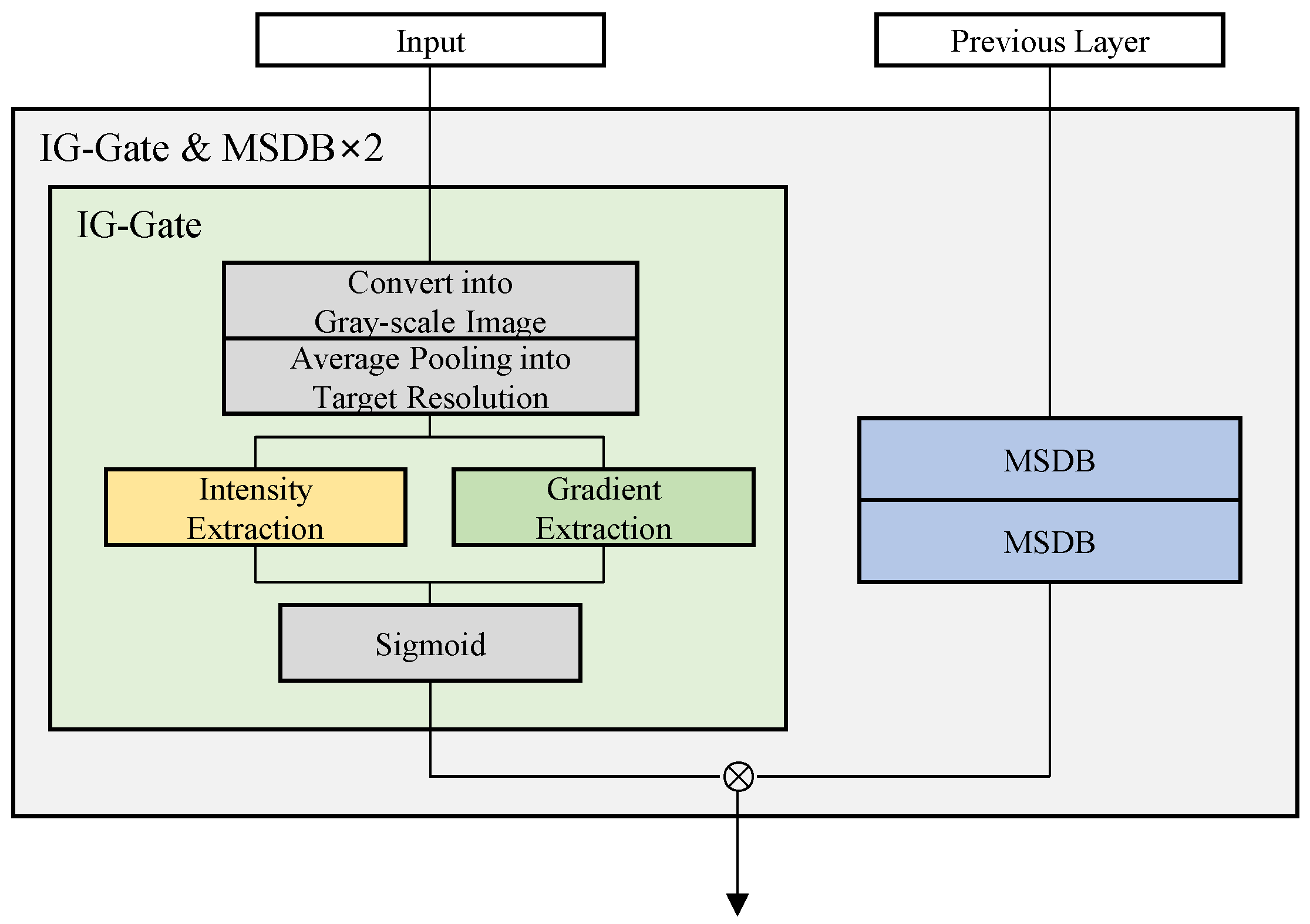
IG-Gate, illustrated in Figure 3, is a parameter-free module that generates a spatial attention score map directly from the original input image $I\in {\mathbb{R}}^{H\times W\times 3}$. The generated score map is used to modulate the features extracted by the MSDBs. To generate a gate $G^{\left(l\right)}$ for the l-th encoder stage with feature map resolution $H^{\prime }\times W^{\prime }$, the input image I is first converted to grayscale, $I_{gray}=\mathcal{T}\left(I\right)$, and downsampled to the target resolution as

$$I_{pool}={\mathcal{P}}_{avg}\left(I_{gray}\right)\in {\mathbb{R}}^{H^{\prime }\times W^{\prime }\times 1}.$$

(12)

From the pooled image, two fundamental low-level feature maps are extracted as a normalized intensity map $F_{int}$ and a gradient magnitude map $F_{grad}$. These cues are chosen because crack pixels are typically distinguished from the background by subtle intensity contrasts and edge-like gradient responses, making them the most decisive evidence for preserving hairline structures. The intensity map is computed by normalizing the pooled image $I_{pool}$ to have a zero mean and unit variance. Let $\mu$ and ${\sigma }^2$ be the mean and variance of $I_{pool}$ over its spatial dimensions. The normalized intensity map is then calculated as

$$F_{int}={\displaystyle \frac{I_{pool}-\mu }{\sqrt{{\sigma }^2+ϵ}}},$$

(13)

where $ϵ$ is a small constant for numerical stability. The gradient magnitude map is computed using Sobel filters. First, we compute the horizontal and vertical gradient components, $G_x$ and $G_y$, as

$$G_x=S_x\ast I_{pool},G_y=S_y\ast I_{pool}.$$

(14)

The gradient magnitude, $F_{grad}$, is then calculated as the L1 norm of these components as

$$F_{grad}=\left|G_x\right|+\left|G_y\right|,$$

(15)

where ∗ denotes the 2D convolution operation. The intensity and gradient maps provide complementary cues for crack evidence. Among possible fusion strategies, we adopt simple element-wise summation for its computational efficiency, yielding the combined score map S as

$$S=F_{int}+F_{grad}.$$

(16)

The map is then passed through a sigmoid function ${\sigma }_{sig}$ to produce the final single-channel spatial gate $G^{\left(l\right)}\in {[0,1]}^{H^{\prime }\times W^{\prime }\times 1}$ as

$$G^{\left(l\right)}={\sigma }_{sig}\left(S\right).$$

(17)

The gate $G^{\left(l\right)}$ is then used to modulate the feature map from the MSDBs, as previously defined in Equation (5). The gating mechanism allows the network to amplify features in regions with strong low-level evidence (high scores) and suppress features in background areas (low scores), effectively preserving critical information without adding learnable parameters.

3.5. Decoder Path and Final Prediction

The decoder path symmetrically recovers spatial resolution to produce the final segmentation map. Let $Y^{\left(l\right)}$ be the output of the l-th decoder stage. For stages $l=L-1,\dots ,1$, the process begins by upsampling the feature map from the deeper layer, $Y^{(l+1)}$, using a transposed convolution, ${\mathcal{U}}^{\left(l\right)}$ as

$$Y_{up}^{\left(l\right)}={\mathcal{U}}^{\left(l\right)}\left(Y^{(l+1)}\right).$$

(18)

Next, the upsampled feature map is concatenated with the corresponding modulated feature map $X_{mod}^{\left(l\right)}$ from the encoder via a skip connection as

$$Y_{cat}^{\left(l\right)}=[Y_{up}^{\left(l\right)},X_{mod}^{\left(l\right)}].$$

(19)

Finally, the fused feature map is passed through a decoding block, ${\mathcal{F}}_{Dec}^{\left(l\right)}$, to refine the features and produce the output for the current stage as

$$Y^{\left(l\right)}={\mathcal{F}}_{Dec}^{\left(l\right)}\left(Y_{cat}^{\left(l\right)}\right).$$

(20)

The final prediction map P is obtained from the output of the last decoder stage, $Y^{\left(1\right)}$, by applying a final $1\times 1$ convolution followed by a sigmoid activation as

$$P={\sigma }_{sig}\left({\mathrm{Conv}}_{1\times 1}\left(Y^{\left(1\right)}\right)\right).$$

(21)

The final operation maps the multi-channel feature map to a single-channel score map, where each pixel value represents the predicted score of belonging to a crack.

4. Experiments

In this section, we provide a comprehensive validation of our proposed EP-REx model. We begin by detailing the experimental setup, followed by quantitative comparisons against state-of-the-art models, a Pareto frontier analysis of the accuracy–efficiency trade-off, an ablation study on core components, and a qualitative analysis of the visual results.

4.1. Experimental Settings

To comprehensively evaluate our proposed method, we compared it against 13 state-of-the-art models covering various approaches in crack segmentation. These baselines were categorized into three groups based on their design objectives and architectures. Lightweight crack segmentation models. We evaluated recent lightweight architectures specifically designed for efficient crack detection. BLCDNet [44] employed biologically inspired mechanisms for contour detection, while CarNet [12] and RHACrackNet [10] proposed efficient CNN architectures for pavement crack detection. DSUNet [4] leveraged depthwise separable convolutions to reduce parameters, and LMNet [36] adopted a modular design for computational efficiency. For a comprehensive comparison, we included models that prioritized segmentation quality for crack detection. CrackFormer II [45] utilizes transformer architecture for pavement crack segmentation, CSNet [11] incorporates multi-scale context with attention mechanisms, and DECSNet [40] employs dual encoders with Haar wavelet-based high-low frequency attention. RSNet [9] extends the U-Net architecture with residual connections for both segmentation and severity assessment, while U-MPSC [46] targeted crack detection in metal pipes. In addition, we included general-purpose lightweight segmentation models to establish broader efficiency baselines. These models were retrained from scratch on the crack datasets with their output layers adapted for binary segmentation, ensuring consistency across comparisons. PIDNet [47] provided real-time semantic segmentation inspired by PID controllers, DSNet [48] introduced novel uses of atrous convolutions, and XYWNet [49] offered edge-detection capabilities through bio-inspired parallel pathways.

We performed comprehensive experiments to demonstrate the effectiveness of our proposed dual-path network. The training process consisted of 100 epochs with a batch size of 4. We utilized the AdamW optimizer configured with a learning rate of $1\times {10}^{-3}$, momentum parameter of 0.9, and weight decay of $1\times {10}^{-4}$. For the loss function, we employed a combination of Dice loss and cross-entropy loss. Our data augmentation strategy incorporated horizontal and vertical flipping along with random rotations at 90°, 180°, and 270° angles. For a thorough evaluation of our approach, we used six widely used public crack segmentation datasets: Ceramic [50], DeepCrack237 [37], Masonry [51], DeepCrack537 [37], CD [32], and CamCrack789 [52], as summarized in

Table 1. Detailed characteristics of crack segmentation datasets.

Dataset	Original Resolution	Input Resolution	# Images	Train/Val/Test
Ceramic [50]	$256\times 256\times 3$	$256\times 256\times 3$	100	60/20/20
DeepCrack237 [37]	$384\times 544\times 3$	$384\times 640\times 3$	237	142/47/48
Masonry [51]	$224\times 224\times 3$	$256\times 256\times 3$	240	144/48/48
DeepCrack537 [37]	$384\times 544\times 3$	$384\times 640\times 3$	537	316/105/106
CD [32]	236–$306\times 256$–$334\times 3$	$384\times 384\times 3$	776	466/155/155
CamCrack789 [52]	$480\times 640\times 3$	$384\times 512\times 3$	789	473/158/158

. These datasets collectively cover a wide range of crack morphologies and imaging conditions. Specifically, Ceramic contains surface-level cracks with relatively uniform textures, while Masonry features fine cracks embedded in highly structured brick backgrounds. DeepCrack237 and DeepCrack537 consist of elongated and connected cracks across concrete surfaces with variable widths and noise conditions. CD includes pavement cracks with diverse widths and irregular branching patterns, and CamCrack789 extends diversity further with high-resolution images of asphalt and road surfaces under varying lighting conditions. This diversity in crack morphology—ranging from hairline cracks to wide fractures, and from homogeneous to highly cluttered backgrounds—provided a challenging and comprehensive benchmark for evaluating the adaptability of the segmentation models. All datasets were split into training, validation, and test sets using a 6:2:2 ratio through random partitioning. To ensure statistical reliability, we repeated each experiment five times independently and report the averaged results. For evaluation, we measured segmentation accuracy using the Intersection-over-Union (IoU), and efficiency using the number of parameters (#Params) and FLOPs.

To systematically evaluate the accuracy–efficiency trade-off of our proposed architecture, we designed and experimented with three distinct variants: Base, Small, and Tiny. These variants were created by progressively reducing both the channel width, controlled by the number of initial feature channels, and the network depth, which was the number of MSDBs per stage. The specific configurations were as follows: The Base variant used 32 initial feature channels and employed a 1–2–2–2 configuration of MSDBs across the four encoder stages. The Small variant reduced the channel width to 28 initial feature channels and used a lighter 1–2–2–1 MSDB configuration, while the Tiny variant was the most compact, with 24 initial feature channels and a 1–1–2–1 MSDB configuration. These design choices allowed for a comprehensive analysis of how performance scaled with model size. Furthermore, paired t-tests were conducted to statistically validate the significance of the performance differences between our proposed models and other methods.

4.2. Experimental Results

The experimental results are organized according to our three model variants: Base, Small, and Tiny. For each variant, we present its IoU performance (

Table 2. IoU performance comparison of the Base model variant against several high-performance segmentation models across six benchmark datasets. Each score represents the average over five independent runs ± for standard deviation. The best results are marked in bold. A triangle (^⯆) indicates statistical significance at the 0.05 level based on paired t-tests against the proposed model.

Model Name	Ceramic	DeepCrack237	Masonry	DeepCrack537	CD	CamCrack789
Proposed (Base)	0.304 ± 0.024	0.793 ± 0.015	0.650 ± 0.017	0.768 ± 0.012	0.762 ± 0.006	0.726 ± 0.004
BLCDNet	0.256 ± 0.027⯆	0.767 ± 0.016⯆	0.579 ± 0.023⯆	0.742 ± 0.015⯆	0.727 ± 0.011⯆	0.710 ± 0.005⯆
CSNet	0.188 ± 0.027⯆	0.717 ± 0.013⯆	0.537 ± 0.008⯆	0.693 ± 0.015⯆	0.621 ± 0.004⯆	0.663 ± 0.005⯆
CarNet	0.254 ± 0.015⯆	0.772 ± 0.012⯆	0.595 ± 0.029⯆	0.740 ± 0.015⯆	0.708 ± 0.005⯆	0.712 ± 0.006⯆
CrackFormer II	0.285 ± 0.025	0.785 ± 0.017	0.632 ± 0.022	0.754 ± 0.015⯆	0.740 ± 0.004⯆	0.720 ± 0.008
DSNet	0.214 ± 0.018⯆	0.760 ± 0.019⯆	0.611 ± 0.023⯆	0.739 ± 0.016⯆	0.696 ± 0.003⯆	0.700 ± 0.003⯆
PIDNet	0.107 ± 0.015⯆	0.687 ± 0.052⯆	0.552 ± 0.049⯆	0.689 ± 0.017⯆	0.630 ± 0.007⯆	0.642 ± 0.011⯆
DSUNet	0.301 ± 0.037	0.779 ± 0.010	0.633 ± 0.023	0.751 ± 0.014⯆	0.749 ± 0.008⯆	0.716 ± 0.005⯆
RSNet	0.252 ± 0.013⯆	0.763 ± 0.018⯆	0.578 ± 0.011⯆	0.725 ± 0.013⯆	0.721 ± 0.011⯆	0.704 ± 0.002⯆
U-MPSC	0.235 ± 0.017⯆	0.683 ± 0.030⯆	0.529 ± 0.033⯆	0.617 ± 0.029⯆	0.682 ± 0.008⯆	0.499 ± 0.079⯆
DECSNet	0.265 ± 0.019	0.774 ± 0.013⯆	0.629 ± 0.015⯆	0.741 ± 0.017⯆	0.712 ± 0.006⯆	0.706 ± 0.005⯆

,

Table 3. IoU performance comparison of the Small model variant against a competing lightweight model across six benchmark datasets. Each score represents the average over five independent runs ± for standard deviation. The best results are marked in bold. A triangle (^⯆) indicates statistical significance at the 0.05 level based on paired t-tests against the proposed model.

Model Name	Ceramic	DeepCrack237	Masonry	DeepCrack537	CD	CamCrack789
Proposed (Small)	0.288 ± 0.026	0.788 ± 0.013	0.644 ± 0.016	0.766 ± 0.016	0.754 ± 0.003	0.725 ± 0.005
RHACrackNet	0.268 ± 0.023	0.770 ± 0.022⯆	0.626 ± 0.017⯆	0.746 ± 0.014⯆	0.734 ± 0.010⯆	0.722 ± 0.004

and

Table 4. IoU performance comparison of the Tiny model variant against competing highly compact models across six benchmark datasets. Each score represents the average over five independent runs ± for standard deviation. The best results are marked in bold. A triangle (^⯆) indicates statistical significance at the 0.05 level based on paired t-tests against the proposed model.

Model Name	Ceramic	DeepCrack237	Masonry	DeepCrack537	CD	CamCrack789
Proposed (Tiny)	0.285 ± 0.041	0.789 ± 0.014	0.643 ± 0.022	0.763 ± 0.015	0.755 ± 0.005	0.719 ± 0.006
LMNet	0.257 ± 0.026	0.782 ± 0.017	0.632 ± 0.023	0.753 ± 0.015⯆	0.739 ± 0.005⯆	0.715 ± 0.007
XYWNet	0.278 ± 0.020	0.777 ± 0.017⯆	0.625 ± 0.028⯆	0.754 ± 0.018⯆	0.737 ± 0.004⯆	0.716 ± 0.005

) and computational complexity (

Table 5. Computational complexity comparison of the Base model variant and larger models. #Params (in millions) remain constant across datasets. FLOPs (in billions) vary based on input dimensions: 256 × 256 for Ceramic/Masonry, 384 × 640 for DeepCrack237/DeepCrack537, 384 × 384 for CD, and 384 × 512 for CamCrack789.

Model	#Params (M)	FLOPs (B)
		Ceramic	DeepCrack237	Masonry	DeepCrack537	CD	CamCrack789
Proposed (Base)	1.71	18.95	71.07	18.95	71.07	42.64	56.85
BLCDNet	2.41	44.43	166.62	44.43	166.62	99.97	133.30
CSNet	3.18	6.46	24.24	6.46	24.24	14.54	19.39
CarNet	4.89	9.56	35.86	9.56	35.86	21.52	28.69
CrackFormer II	4.96	40.16	150.60	40.16	150.60	90.36	120.48
DSNet	6.55	13.91	52.12	13.91	52.12	31.28	41.70
PIDNet	7.62	2.95	11.04	2.95	11.04	6.63	8.83
DSUNet	11.59	45.20	169.26	45.20	169.26	101.60	135.43
RSNet	13.09	163.80	614.26	163.80	614.26	368.56	491.41
U-MPSC	36.07	132.63	497.37	132.63	497.37	298.42	397.90
DECSNet	47.41	19.61	73.54	19.61	73.54	44.12	58.83

,

Table 6. Computational complexity comparison of the Small model variant and larger models. #Params (in millions) remain constant across datasets. FLOPs (in billions) vary based on input dimensions: 256 × 256 for Ceramic/Masonry, 384 × 640 for DeepCrack237/DeepCrack537, 384 × 384 for CD, and 384 × 512 for CamCrack789.

Model	#Params (M)	FLOPs (B)
		Ceramic	DeepCrack237	Masonry	DeepCrack537	CD	CamCrack789
Proposed (Small)	0.99	12.80	47.99	12.80	47.99	28.79	38.39
RHACrackNet	1.67	4.52	16.94	4.52	16.94	10.16	13.55

and

Table 7. Computational complexity comparison of the Tiny model variant and larger models. #Params (in millions) remain constant across datasets. FLOPs (in billions) vary based on input dimensions: 256 × 256 for Ceramic/Masonry, 384 × 640 for DeepCrack237/DeepCrack537, 384 × 384 for CD, and 384 × 512 for CamCrack789.

Model	#Params (M)	FLOPs (B)
		Ceramic	DeepCrack237	Masonry	DeepCrack537	CD	CamCrack789
Proposed (Tiny)	0.69	8.12	30.45	8.12	30.45	18.27	24.36
LMNet	0.83	16.13	60.50	16.13	60.50	36.30	48.40
XYWNet	0.89	7.95	29.79	7.95	29.79	17.88	23.84

) in dedicated tables. Each variant was benchmarked against state-of-the-art models of a similar or larger scale, focusing on the trade-off between segmentation accuracy and efficiency.

Table 2 presents the IoU performance of our Base model against a broad range of state-of-the-art methods, including high-performance crack-specific and general-purpose segmentation models. The proposed Base model consistently achieved the highest IoU scores across all six datasets, demonstrating its superior accuracy. Specifically, it obtained an IoU of 0.304 on Ceramic, 0.793 on DeepCrack237, 0.650 on Masonry, 0.768 on DeepCrack537, 0.762 on CD, and 0.726 on CamCrack789. The performance gains were statistically significant ($p<0.05$) against the majority of competing models. Our model consistently outperformed its closest competitors, CrackFormer II and DSUNet. For instance, it achieved a notable +0.017 IoU improvement over DSUNet on the Masonry dataset.

Table 5 details the computational complexity of these models. Our Base model, with only 1.71 M parameters, was significantly more lightweight than all other models in this comparison group, as several competing models had over 4 M parameters (e.g., CrackFormer II and DSUNet) and some exceeded 10 M (e.g., RSNet and U-MPSC). In terms of FLOPs, our model was also highly efficient, requiring fewer computations than high-performing competitors such as CrackFormer II and DSUNet. While some models, such as CSNet and PIDNet, had lower FLOPs, their IoU scores were substantially lower, placing them at a much less favorable point on the accuracy–efficiency curve. These results demonstrated that our Base model achieved a favorable accuracy–efficiency trade-off, delivering consistently superior accuracy with substantially fewer parameters and FLOPs compared to existing methods, as confirmed across six diverse crack segmentation datasets.

To evaluate our architecture in a more resource-constrained setting, we compared our Small variant against RHACrackNet, a recent lightweight model. As shown in Table 3, the Proposed (Small) model surpassed RHACrackNet in IoU on all six datasets. The performance margins were statistically significant on the DeepCrack237, Masonry, DeepCrack537, and CD datasets, with improvements of +0.018, +0.018, +0.020 IoU, and +0.020 IoU, respectively. The complexity comparison in Table 6 revealed an interesting trade-off. Our Small model was more parameter-efficient, with only 0.99 M parameters compared to the 1.67 M of RHACrackNet. This highlighted the exceptional parameter efficiency of the proposed model, demonstrating that our architecture achieved higher accuracy with a significantly smaller memory footprint, which ultimately offered a better parameter-to-performance ratio. For applications where model storage was a primary constraint, our Small variant presented a more compelling option, although this advantage came with a trade-off in computational cost (12.80 B vs. 4.52 B FLOPs in Ceramic/Masonry).

In the category of highly compact models, we compared our Tiny model against two strong competitors, LMNet and XYWNet. The IoU results in Table 4 showed that our Tiny variant consistently achieved the best performance, outperforming both baselines on all six datasets. The improvements were statistically significant against XYWNet on four of the six datasets and against LMNet on the DeepCrack537 and CD datasets. From a complexity standpoint (Table 7), the Proposed (Tiny) model was the most efficient in this group. With only 0.69 M parameters, it was lighter than both LMNet (0.83 M) and XYWNet (0.89 M). Furthermore, its FLOPs (8.12 B) were nearly identical to the 7.95 B of XYWNet and less than half of the 16.13 B of LMNet on the Ceramic and Masonry. In summary, the Proposed (Tiny) model achieved the best accuracy–efficiency trade-off in its category by delivering the highest IoU scores while being the most parameter-efficient and maintaining a highly competitive computational cost.

4.3. Efficiency Analysis

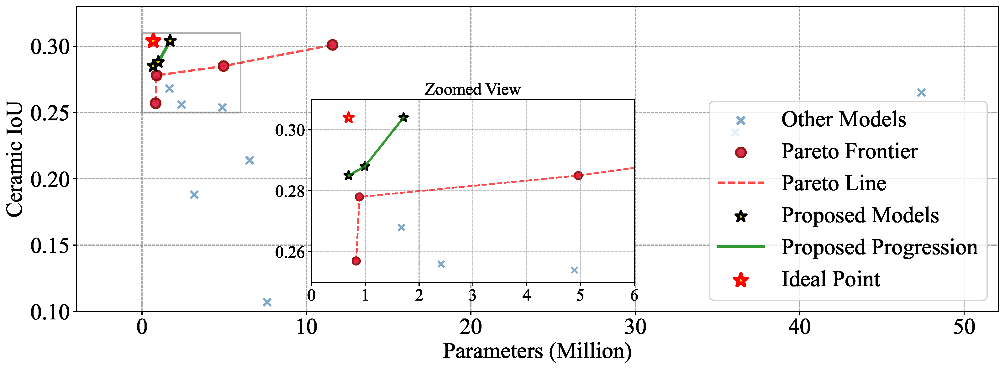
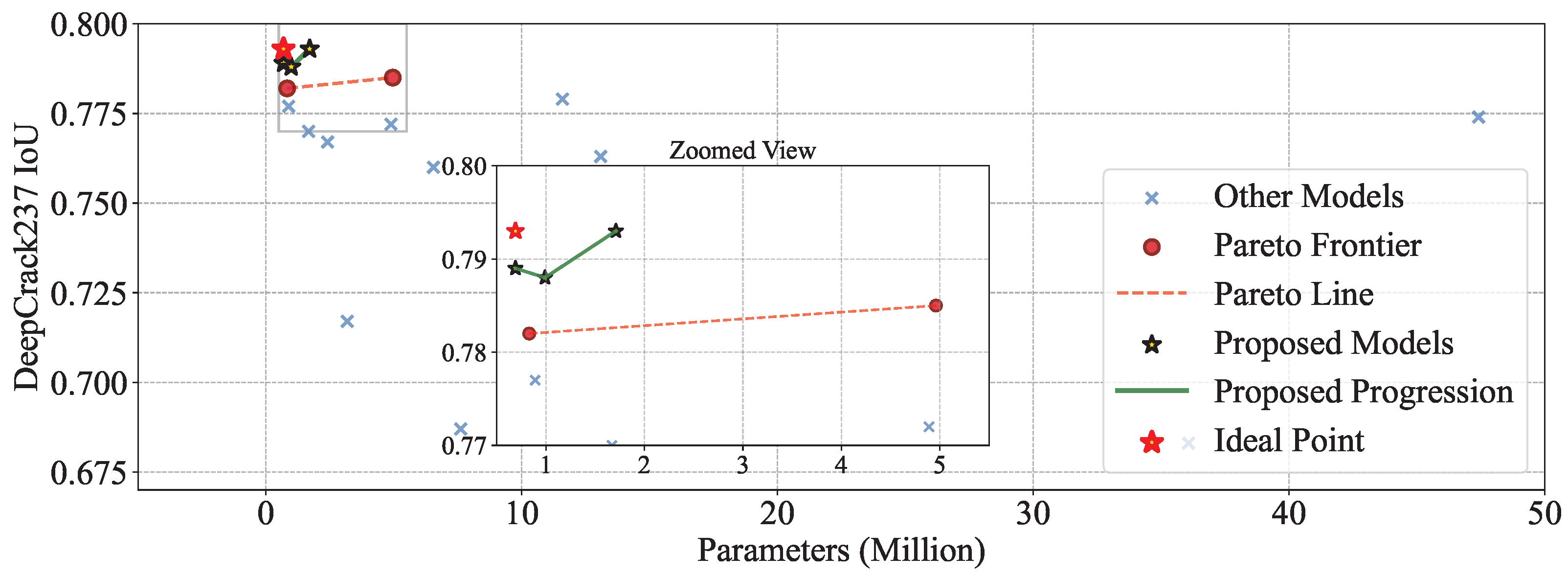
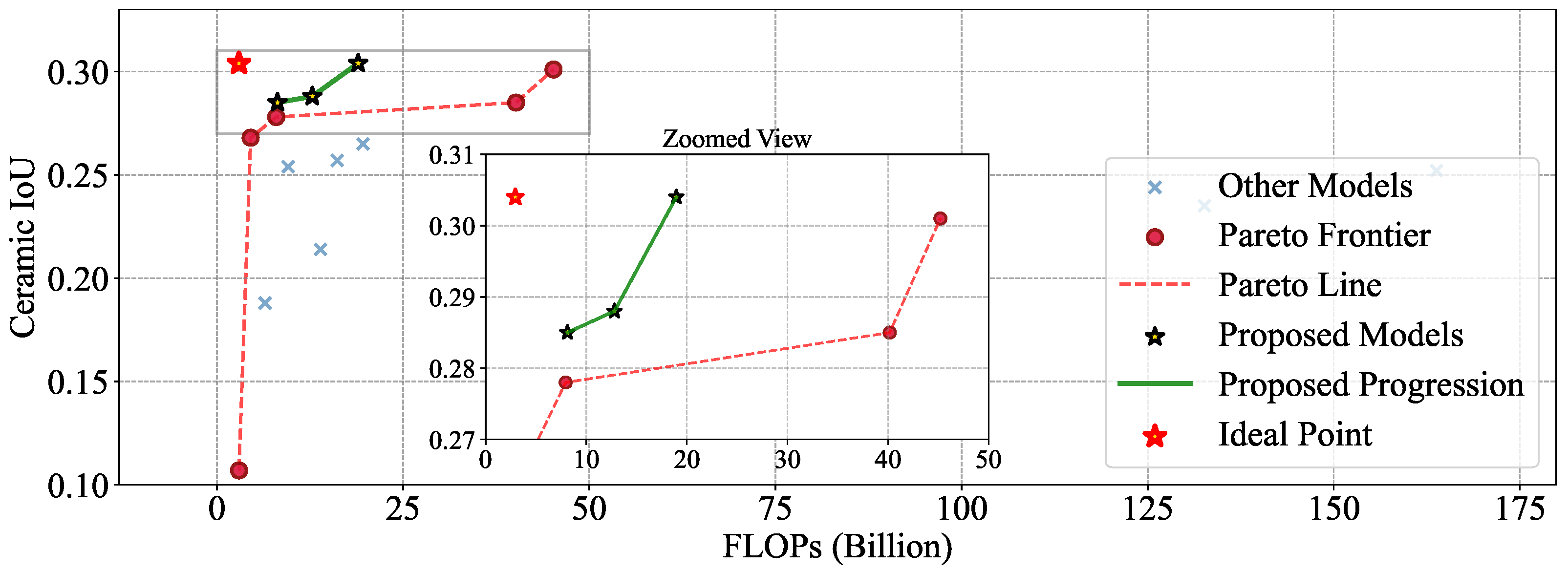
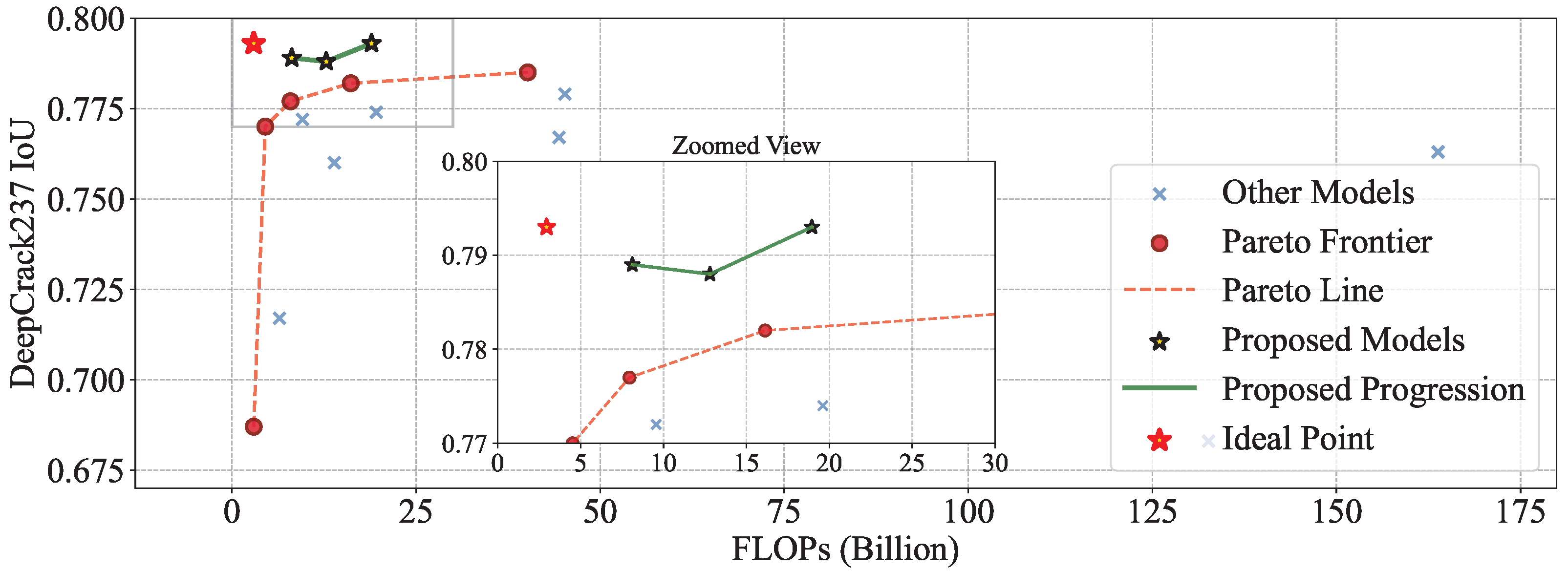
To demonstrate the practical applicability of our proposed method, we conducted a comprehensive efficiency analysis comparing model complexity against segmentation performance. Figure 4, Figure 5, Figure 6 and Figure 7 present Pareto frontier analysis for two representative datasets: Ceramic and DeepCrack237, examining trade-offs between #Params, computational cost (FLOPs), and IoU performance. The analysis revealed several key insights into the efficiency characteristics of crack segmentation models. Our proposed approach demonstrated superior efficiency across multiple scales, with our Base, Small, and Tiny variants (connected by the green line) achieving competitive performance while maintaining lower computational requirements compared to existing methods.

In the parameter efficiency analysis (Figure 4 and Figure 5), our method consistently outperformed competing approaches. On the Ceramic dataset, our Tiny variant achieved comparable performance to much larger models while using significantly fewer parameters. The progression from Tiny to Base variants showed a controlled trade-off between model complexity and performance, allowing practitioners to select the appropriate variant based on their computational constraints.

The computational efficiency analysis using FLOPs (Figure 6 and Figure 7) further validated the efficiency of our approach. The Pareto frontier analysis identified the best trade-off points among existing methods (circles and dashed line), while our proposed models consistently achieved better efficiency ratios. Notably, our Small and Tiny variants often achieved performance comparable to much more computationally expensive models, making them particularly suitable for resource-constrained applications.

The consistent efficiency advantages across both datasets demonstrated the generalizability of our approach. While some competing methods achieved higher peak performance, they did so at the cost of significantly increased computational requirements. Our method provided a more balanced solution, offering practitioners flexible options that maintained high accuracy while respecting computational constraints. This efficiency analysis underscored the practical value of our proposed method for real-world deployment scenarios where computational resources were limited, such as edge computing applications or real-time inspection systems.

4.4. Ablation Study

To validate the effectiveness of our two core components, MSDB and IG-Gate, we conducted a comprehensive ablation study. We evaluated four configurations on four distinct datasets: a baseline model with both modules disabled, and three variants with each module enabled individually and then jointly. The baseline model replaced the MSDBs with standard bottleneck blocks of a similar computational cost. The results, summarized in

Table 8. Ablation study of the MSDB and IG-Gate modules on four datasets. Adding both modules yields the best IoU across datasets. Values are mean ± standard deviation.

Modules		IoU
MSDB	IG-Gate	Ceramic	DeepCrack237	Masonry	DeepCrack537
✓	✓	0.295 ± 0.023	0.791 ± 0.014	0.650 ± 0.022	0.762 ± 0.011
✓	×	0.286 ± 0.007	0.786 ± 0.015	0.646 ± 0.016	0.762 ± 0.013
×	✓	0.291 ± 0.007	0.779 ± 0.009	0.617 ± 0.036	0.750 ± 0.022
×	×	0.266 ± 0.032	0.775 ± 0.015	0.632 ± 0.033	0.755 ± 0.017

, clearly demonstrated the individual and synergistic contributions of our proposed modules. The baseline model (×, ×) provided a solid performance foundation. Enabling MSDB alone (✓, ×) consistently improved the IoU over the baseline across most datasets, validating its effectiveness in expanding the receptive field and capturing better contextual features. Similarly, enabling IG-Gate alone (×, ✓) also showed a performance gain, particularly on the Ceramic and Masonry datasets, which highlighted its ability to preserve crucial low-level evidence that might otherwise have been lost. The full model configuration with both MSDB and IG-Gate enabled (✓, ✓) achieved the highest IoU on all four datasets. This superior performance underscored the synergistic relationship between the two components: MSDB efficiently expanded the receptive field for learning vital crack characteristics, and IG-Gate ensured that this process was guided by the most salient input evidence. This combination allowed the model to resolve the context–evidence dilemma more effectively than either component could alone, leading to more accurate and robust segmentation results.

To further clarify the contribution of each module, we provide a detailed comparison of computational complexity and accuracy in

Table 9. Computational complexity comparison for ablation study. #Params (in millions) remain constant across datasets. FLOPs (in billions) vary based on input dimensions: 256 × 256 for Ceramic/Masonry and 384 × 640 for DeepCrack237/DeepCrack537.

Model	#Params (M)	FLOPs (B)
		Ceramic	DeepCrack237	Masonry	DeepCrack537
Proposed	1.71	18.95	71.07	18.95	71.07
MSDB Only	1.71	18.95	71.07	18.95	71.07
IG-Gate Only	2.62	23.74	89.02	23.74	89.02
Baseline	2.62	23.74	89.02	23.74	89.02

. Replacing the residual bottlenecks of the baseline with MSDB reduced the parameter count from 2.62 M to 1.71 M and lowered FLOPs by about 20% (e.g., from 23.74 B to 18.95 B for $256\times 256$ inputs and from 89.02 B to 71.07 B for $384\times 640$ inputs) while also improving segmentation accuracy. In contrast, IG-Gate did not increase the parameters or FLOPs, since it is a parameter-free spatial gate. Its effectiveness is reflected in accuracy gains: when combined with MSDB, the IoU improved by +0.009 on Ceramic, +0.005 on DeepCrack237, and +0.004 on Masonry, without incurring additional computational cost. These results confirmed that the lightweightness of our model mainly originated from the replacement of residual bottlenecks with MSDB, while IG-Gate contributed complementary performance improvements at negligible overhead.

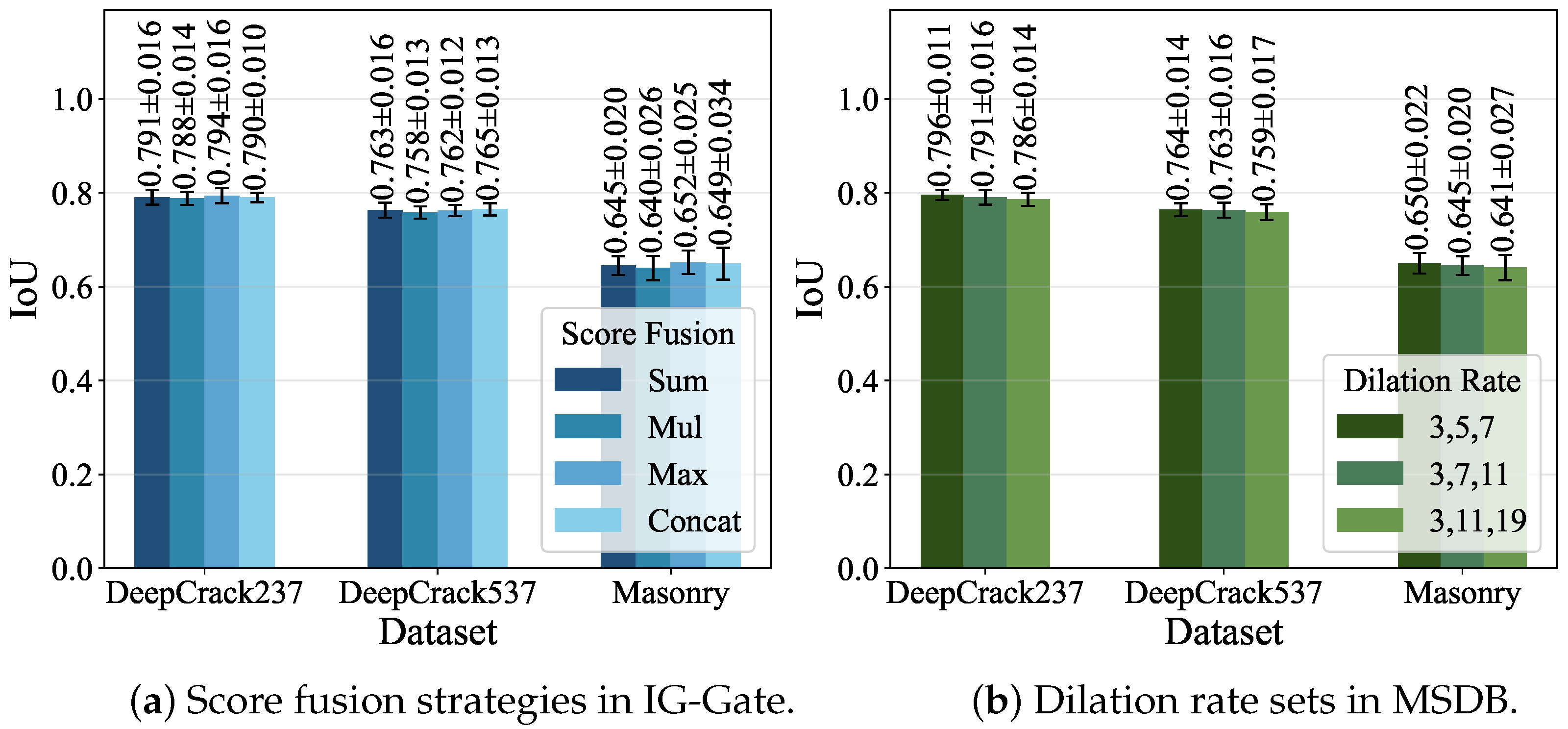
We further examined alternative fusion strategies for combining the normalized intensity and gradient maps in IG-Gate, as illustrated in Figure 8a. Specifically, we compared four strategies: (i) Sum, which directly added the two maps and applied the combined score to all channels; (ii) Mul, which multiplied the two maps to further emphasize overlapping strong responses; (iii) Max, which selected the maximum response at each pixel location; and (iv) Concat, where the feature channels were split in half, with the intensity map applied to the first half and the gradient map applied to the second half. The results, reported in Figure 8a, show minimal performance differences across the strategies. For example, on DeepCrack237, the IoU scores are 0.791, 0.788, 0.794, and 0.790 for Sum, Mul, Max, and Concat, respectively. Similar trends were observed on DeepCrack537 (0.763; 0.758; 0.762; 0.765) and Masonry (0.645; 0.640; 0.652; 0.649). Given the comparable performance, we adopted the Sum strategy, as it offered the simplest and most numerically stable implementation without incurring additional complexity.

Figure 8b shows the ablation study on different sets of dilation rates in MSDB. The set $1,3,5$ was empirically determined during the prototyping stage of our model and adopted in the main experiments. Although $1,2,3$ showed marginally higher performance (e.g., 0.796 vs. 0.791 IoU on DeepCrack237), the difference was not substantial. Interestingly, excessively large dilation gaps (e.g., $3,11,19$) degraded performance, suggesting that overly sparse sampling weakened the ability of the model to follow the continuity of elongated cracks. This implied that dilation rate selection should be treated as a tunable hyperparameter, and moderate expansions could better preserve crack structures.

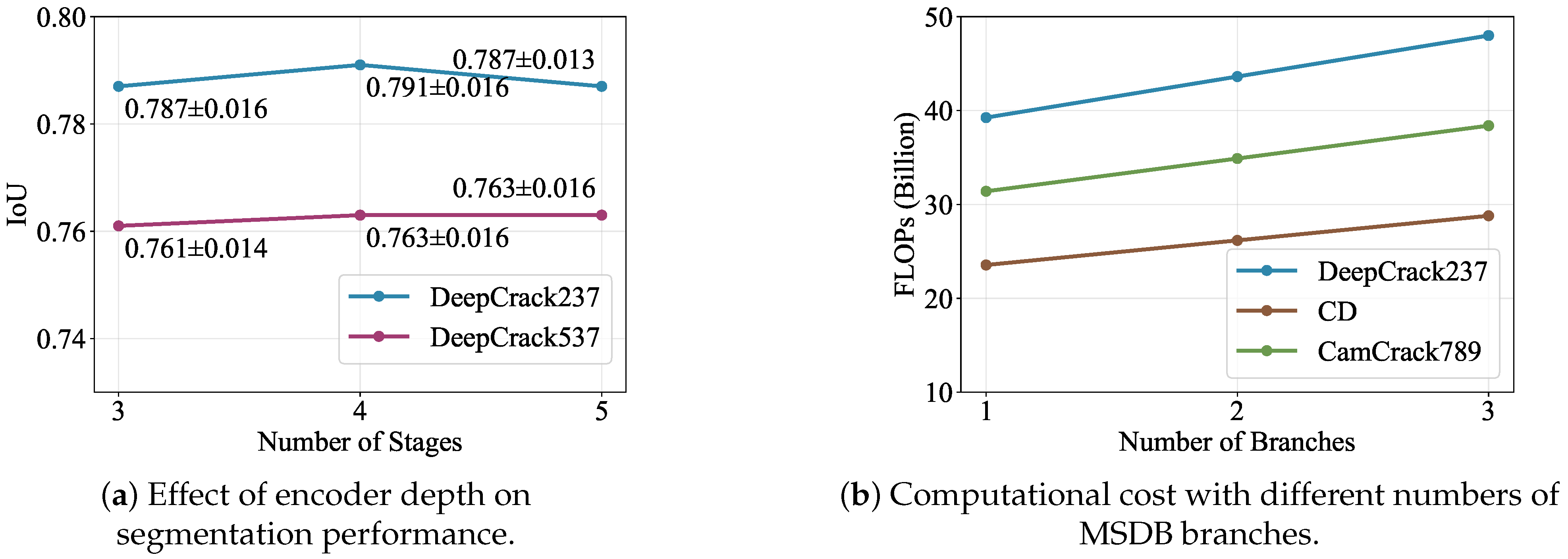
Figure 9a presents the hyperparameter analysis for the number of encoder stages, conducted on three representative datasets (DeepCrack237 and DeepCrack537). The results showed that performance improved when increasing the depth from three to four stages, with IoU rising from 0.787 to 0.791 on DeepCrack237 and from 0.761 to 0.763 on DeepCrack537. However, further increasing the depth to five stages did not yield additional gains and, in some cases, slightly degraded performance (e.g., DeepCrack237: 0.787). These results indicate that three max-pooling operations (i.e., four encoder stages) provided the most favorable trade-off, supporting our architectural choice. Unlike traditional crack segmentation architectures [36,45], which often rely on four or five downsampling operations to expand the receptive field at deeper layers, our study showed that such excessive downsampling did not consistently improve crack segmentation.

To further quantify the FLOPs increase caused by the parallel structure, we analyzed the effect of varying the number of MSDB branches in the Small version. As shown in Figure 9b, FLOPs increased almost linearly with the number of branches across datasets (DeepCrack237, CD, and CamCrack789), confirming that the parallel dilated convolution design was the primary contributor to the higher computational cost. Nevertheless, when compared with RHACrackNet, our model still required more FLOPs, suggesting that additional efficiency strategies beyond branch reduction were needed for further improvement.

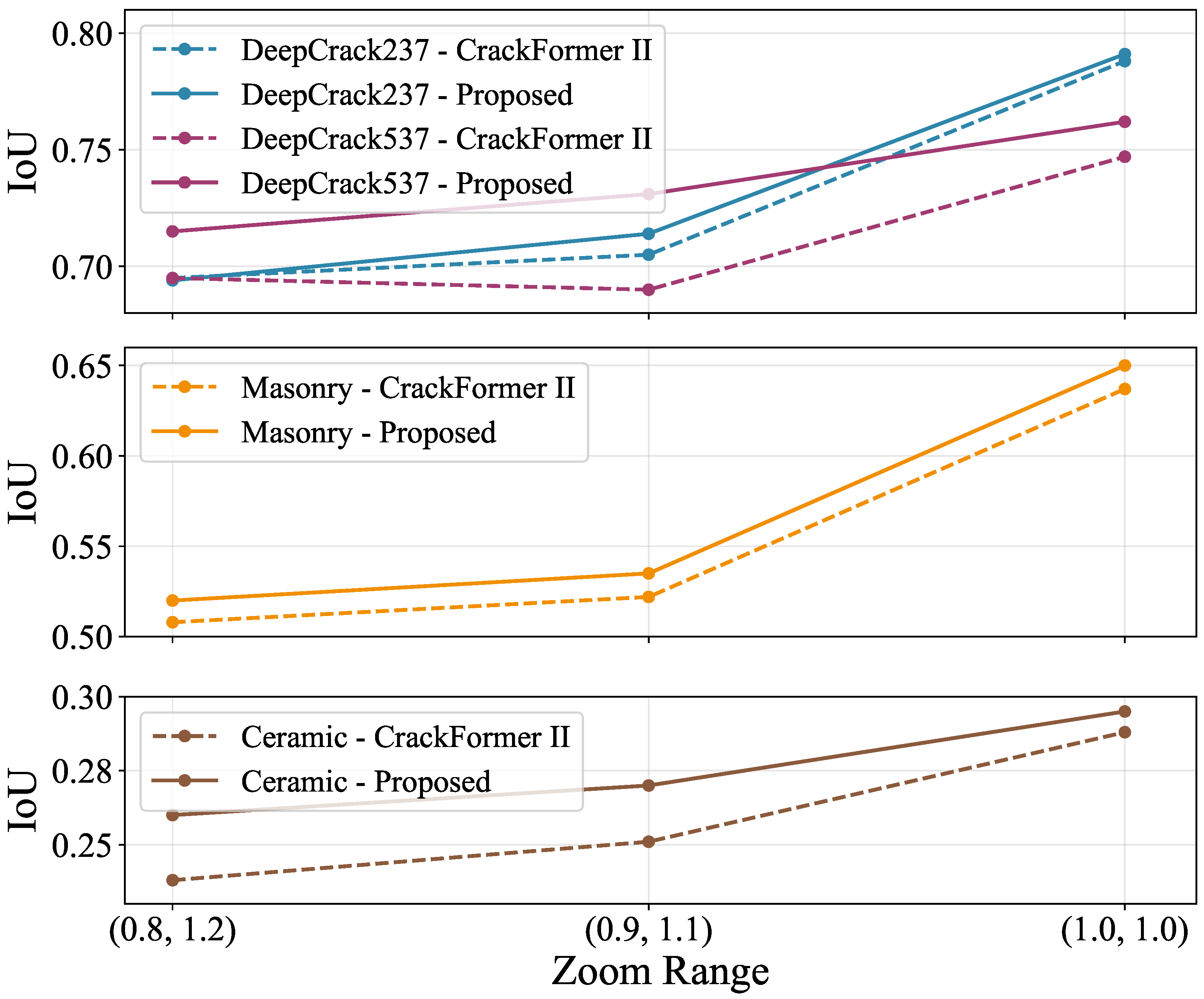
In real-world scenarios, such as UAV- or robot-based inspection, the distance between the imaging device and the target surface could vary substantially, which, in turn, can alter the apparent scale of cracks. To examine the robustness of our model under such conditions, we conducted an evaluation using random zoom augmentations at test time. Specifically, we compared the proposed model with CrackFormer II across three zoom ranges: $(0.8,1.2)$, $(0.9,1.1)$, and $(1.0,1.0)$, where a wider range represented more challenging scale variations. The results, illustrated in Figure 10, show that as the zoom range widened, both models experienced gradual IoU degradation. Nevertheless, the proposed model consistently exhibited a smaller performance drop compared to CrackFormer II across all datasets, highlighting its enhanced robustness against scale changes. This suggests that the combination of multi-scale receptive field expansion via MSDB and low-level guidance from IG-Gate enables our network to better preserve crack continuity, even when scale variations were present.

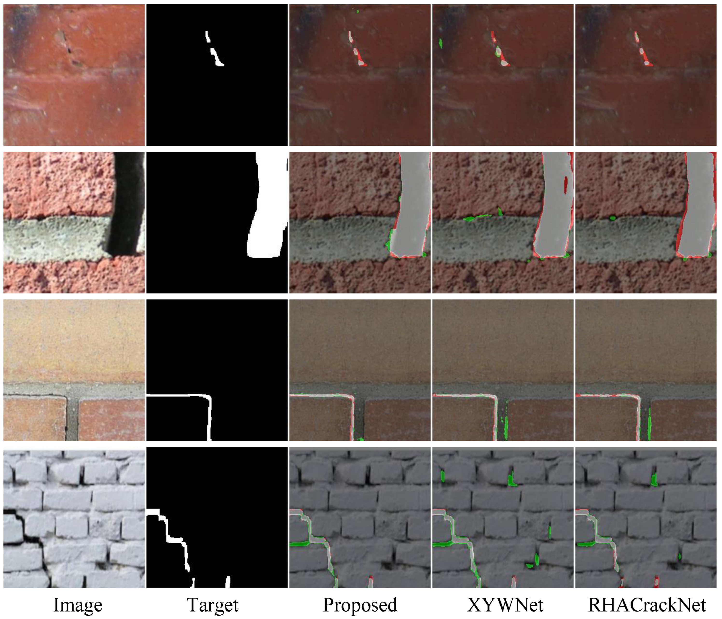
Figure 11 presents the qualitative results for the Masonry dataset. In challenging cases where brick seams or surface textures resembled cracks, existing lightweight models, such as XYWNet and RHACrackNet, often misclassified these patterns as cracks, leading to spurious detections. In contrast, the proposed EP-REx leveraged evidence-preserving gating to anchor receptive-field expansion on raw intensity and gradient cues, thereby suppressing crack-like background responses while maintaining the continuity of actual crack structures. This demonstrated the advantage of our evidence-preserving design in improving robustness against visually similar but irrelevant patterns.

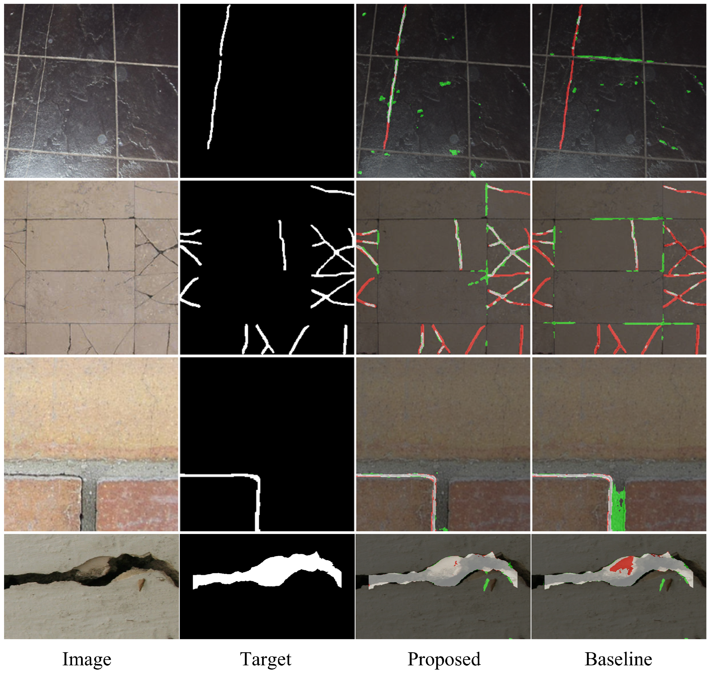
To further validate the contribution of MSDB and IG-Gate in expanding the receptive field, we provide qualitative comparisons in Figure 12. The baseline corresponds to the ablation setting in which both MSDB and IG-Gate were removed. In the first row, the baseline failed to capture fine cracks on dark tiles, whereas the proposed model detected them more continuously. In the second row, when handling complex branching cracks, the proposed model suppressed false positives and better preserved elongated structures. In the third row, for thin cracks on brick textures, the proposed model reduced background noise and maintained sharper boundaries. In the fourth row, which includes wide cracks with irregular shapes, the proposed model more accurately delineated crack regions with fewer missing parts. These comparisons demonstrate that MSDB and IG-Gate improved crack continuity and robustness across different scenarios.

5. Conclusions

In this paper, we present EP-REx, a crack segmentation network that combines multi-scale dilated depthwise convolutions with an input-guided gate to efficiently expand receptive fields while preserving critical evidence from the input. Through extensive experiments on six benchmark datasets, EP-REx consistently achieved the highest accuracy. Although our models do not yield the lowest FLOPs among compact baselines, they provide a balanced design between accuracy and computational cost. EP-REx achieves a balanced design, combining strong accuracy with computational efficiency.

Despite its favorable balanced accuracy–cost design, one limitation is the computational cost in terms of FLOPs. While our Small variant achieves superior accuracy and parameter efficiency compared to RHACrackNet, its FLOPs remain higher, partly due to the parallel dilated convolution structure in the MSDB. Although this design is central to achieving strong accuracy, future work should explore additional optimizations to further reduce computational overhead. Moreover, while EP-REx generally achieves higher segmentation accuracy than existing methods, in some cases, the improvement margin is modest (e.g., within 0.01–0.02 IoU), suggesting that practical gains may depend on the deployment scenario. In addition, our study adopted simple data augmentation strategies (e.g., flipping and rotation), and exploring morphology-oriented augmentations tailored to crack structures remains an important direction for future research. Finally, while EP-REx demonstrates favorable accuracy–efficiency characteristics, we acknowledge that real-world deployment tests on edge devices, such as drones or mobile robots, were not conducted in this study, and validating runtime performance on physical hardware remains an important direction for future research.

References

1. Zou, Q.; Cao, Y.; Li, Q.; Mao, Q.; Wang, S. CrackTree: Automatic crack detection from pavement images. Pattern Recognit. Lett. 2012, 33, 227–238. [Google Scholar] [CrossRef]
2. Zou, Q.; Zhang, Z.; Li, Q.; Qi, X.; Wang, Q.; Wang, S. Deepcrack: Learning hieraarchical convolutional features for crack detection. IEEE Trans. Image Process. 2018, 28, 1498–1512. [Google Scholar] [CrossRef]
3. Dong, C.Z.; Catbas, F.N. A review of computer vision–based structural health monitoring at local and global levels. Struct. Health Monit. 2021, 20, 692–743. [Google Scholar] [CrossRef]
4. Yu, Y.; Zhang, Y.; Yu, J.; Yue, J. Lightweight decoder U-net crack segmentation network based on depthwise separable convolution. Multimedia Syst. 2024, 30, 295. [Google Scholar] [CrossRef]
5. Wang, F.; Wang, Z.; Wu, X.; Wu, D.; Hu, H.; Liu, X.; Zhou, Y. E2S: A UAV-Based Levee Crack Segmentation Framework Using the Unsupervised Deblurring Technique. Remote Sens. 2025, 17, 935. [Google Scholar] [CrossRef]
6. Zhang, Y.; Xu, Y.; Martinez-Rau, L.S.; Vu, Q.N.P.; Oelmann, B.; Bader, S. On-Device Crack Segmentation for Edge Structural Health Monitoring. arXiv 2025, arXiv:2505.07915. [Google Scholar] [CrossRef]
7. Kim, Y.; Yi, S.; Ahn, H.; Hong, C.H. Accurate Crack Detection Based on Distributed Deep Learning for IoT Environment. Sensors 2023, 2, 858. [Google Scholar] [CrossRef] [PubMed]
8. Howard, A.; Sandler, M.; Chu, G.; Chen, L.C.; Chen, B.; Tan, M.; Wang, W.; Zhu, Y.; Pang, R.; Vasudevan, V.; et al. Searching for MobileNetV3. In Proceedings of the IEEE/CVF International Conference on Computer Vision (ICCV), Seoul, Republic of Korea, 27 October–2 November 2019. [Google Scholar]
9. Ali, L.; AlJassmi, H.; Swavaf, M.; Khan, W.; Alnajjar, F. RS-Net: Residual Sharp U-Net architecture for pavement crack segmentation and severity assessment. J. Big Data 2024, 11, 116. [Google Scholar] [CrossRef]
10. Zhu, G.; Liu, J.; Fan, Z.; Yuan, D.; Ma, P.; Wang, M.; Sheng, W.; Wang, K.C. A lightweight encoder–decoder network for automatic pavement crack detection. Comput.-Aided Civ. Infrastruct. Eng. 2024, 39, 1743–1765. [Google Scholar] [CrossRef]
11. Liang, J. CNN-based network with multi-scale context feature and attention mechanism for automatic pavement crack segmentation. Autom. Constr. 2024, 164, 105482. [Google Scholar] [CrossRef]
12. Li, K.; Yang, J.; Ma, S.; Wang, B.; Wang, S.; Tian, Y.; Qi, Z.; Tian, Y. Rethinking Lightweight Convolutional Neural Networks for Efficient and High-Quality Pavement Crack Detection. IEEE Trans. Intell. Transp. Syst. 2024, 25, 237–250. [Google Scholar] [CrossRef]
13. Wang, Z.; Ji, S. Smoothed Dilated Convolutions for Improved Dense Prediction. In Proceedings of the 24th ACM SIGKDD International Conference on Knowledge Discovery and Data Mining (KDD ’18), London, UK, 19–23 August 2018; pp. 2486–2495. [Google Scholar] [CrossRef]
14. Long, J.; Shelhamer, E.; Darrell, T. Fully convolutional networks for semantic segmentation. In Proceedings of the 2015 IEEE Conference on Computer Vision and Pattern Recognition (CVPR), Boston, MA, USA, 7–12 June 2015; pp. 3431–3440. [Google Scholar]
15. Ronneberger, O.; Fischer, P.; Brox, T. U-Net: Convolutional Networks for Biomedical Image Segmentation. In Proceedings of the Medical Image Computing and Computer-Assisted Intervention—MICCAI 2015, Munich, Germany, 5–9 October 2015; pp. 234–241. [Google Scholar] [CrossRef]
16. Duarte, K.T.; Gobbi, D.G.; Sidhu, A.S.; McCreary, C.R.; Saad, F.; Camicioli, R.; Smith, E.E.; Frayne, R. Segmenting white matter hyperintensities in brain magnetic resonance images using convolution neural networks. Pattern Recognit. Lett. 2023, 175, 90–94. [Google Scholar] [CrossRef]
17. Morita, D.; Kawarazaki, A.; Koimizu, J.; Tsujiko, S.; Soufi, M.; Otake, Y.; Sato, Y.; Numajiri, T. Automatic orbital segmentation using deep learning-based 2D U-net and accuracy evaluation: A retrospective study. J. Cranio Maxillofac. Surg. 2023, 51, 609–613. [Google Scholar] [CrossRef]
18. Chen, L.C.; Zhu, Y.; Papandreou, G.; Schroff, F.; Adam, H. Encoder-Decoder with Atrous Separable Convolution for Semantic Image Segmentation. In Proceedings of the European Conference on Computer Vision (ECCV 2018), Munich, Germany, 8–14 September 2018; pp. 833–851. [Google Scholar]
19. Xie, E.; Wang, W.; Yu, Z.; Anandkumar, A.; Alvarez, J.M.; Luo, P. SegFormer: Simple and efficient design for semantic segmentation with transformers. In Proceedings of the Advances in Neural Information Processing Systems 34, Virtual, 6–14 December 2021. [Google Scholar]
20. Li, T.; Cui, Z.; Zhang, H. Semantic segmentation feature fusion network based on transformer. Sci. Rep. 2025, 15, 6110. [Google Scholar] [CrossRef]
21. Fu, B.; Peng, Y.; He, J.; Tian, C.; Sun, X.; Wang, R. HmsU-Net: A hybrid multi-scale U-net based on a CNN and transformer for medical image segmentation. Comput. Biol. Med. 2024, 170, 108013. [Google Scholar] [CrossRef]
22. Heidari, M.; Kazerouni, A.; Soltany, M.; Azad, R.; Aghdam, E.K.; Cohen-Adad, J.; Merhof, D. HiFormer: Hierarchical Multi-Scale Representations Using Transformers for Medical Image Segmentation. In Proceedings of the 2023 IEEE Winter Conference on Applications of Computer Vision (WACV), Waikoloa, HI, USA, 2–7 January 2023; pp. 6202–6212. [Google Scholar]
23. Sze, V.; Chen, Y.H.; Yang, T.J.; Emer, J.S. Efficient Processing of Deep Neural Networks: A Tutorial and Survey. Proc. IEEE 2017, 105, 2295–2329. [Google Scholar] [CrossRef]
24. Ma, N.; Zhang, X.; Zheng, H.T.; Sun, J. ShuffleNet V2: Practical Guidelines for Efficient CNN Architecture Design. In Proceedings of the European Conference on Computer Vision (ECCV 2018), Munich, Germany, 8–14 September2018; pp. 122–138. [Google Scholar]
25. Tan, M.; Le, Q. EfficientNet: Rethinking Model Scaling for Convolutional Neural Networks. In Proceedings of the 36th International Conference on Machine Learning (ICML-19), Long Beach, CA, USA, 9–15 June 2019; Chaudhuri, K., Salakhutdinov, R., Eds.; Volume 97, pp. 6105–6114. [Google Scholar]
26. Howard, A.G.; Zhu, M.; Chen, B.; Kalenichenko, D.; Wang, W.; Weyand, T.; Andreetto, M.; Adam, H. Mobilenets: Efficient convolutional neural networks for mobile vision applications. arXiv 2017, arXiv:1704.04861. [Google Scholar] [CrossRef]
27. Zhang, X.; Zhou, X.; Lin, M.; Sun, J. ShuffleNet: An Extremely Efficient Convolutional Neural Network for Mobile Devices. In Proceedings of the 2018 IEEE/CVF Conference on Computer Vision and Pattern Recognition (CVPR), Salt Lake City, UT, USA, 18–22 June 2018; pp. 6848–6856. [Google Scholar]
28. Han, S.; Pool, J.; Tran, J.; Dally, W. Learning both Weights and Connections for Efficient Neural Networks. Adv. Neural. Inf. Process Syst. 2015, 28, 1135–1143. [Google Scholar]
29. Yang, C.; Zhao, P.; Li, Y.; Niu, W.; Guan, J.; Tang, H.; Qin, M.; Ren, B.; Lin, X.; Wang, Y.; et al. Pruning parameterization with bi-level optimization for efficient semantic segmentation on the edge. In Proceedings of the 2023 IEEE/CVF Conference on Computer Vision and Pattern Recognition (CVPR), Vancouver, BC, Canada, 18–22 June 2023; pp. 15402–15412. [Google Scholar]
30. Liu, Y.; Chen, K.; Liu, C.; Qin, Z.; Luo, Z.; Wang, J. Structured Knowledge Distillation for Semantic Segmentation. In Proceedings of the 2019 IEEE/CVF Conference on Computer Vision and Pattern Recognition (CVPR), Long Beach, CA, USA, 16–20 June 2019. [Google Scholar]
31. Dung, D.V.; Anh, L.D. Autonomous concrete crack detection using deep fully convolutional neural network. Autom. Constr. 2019, 99, 52–58. [Google Scholar] [CrossRef]
32. Yang, X.; Li, H.; Yu, Y.; Luo, X.; Huang, T.; Yang, X. Automatic Pixel-Level Crack Detection and Measurement Using Fully Convolutional Network. Comput.-Aided Civ. Infrastruct. Eng. 2018, 33, 1090–1109. [Google Scholar] [CrossRef]
33. Li, G.; Ma, B.; He, S.; Ren, X.; Liu, Q. Automatic Tunnel Crack Detection Based on U-Net and a Convolutional Neural Network with Alternately Updated Clique. Sensors 2020, 20, 717. [Google Scholar] [CrossRef] [PubMed]
34. Shi, Y.; Cui, L.; Qi, Z.; Meng, F.; Chen, Z. Automatic road crack detection using random structured forests. IEEE Trans. Intell. Transp. Syst. 2016, 17, 3434–3445. [Google Scholar] [CrossRef]
35. Liu, H.; Miao, X.; Mertz, C.; Xu, C.; Kong, H. CrackFormer: Transformer Network for Fine-Grained Crack Detection. In Proceedings of the 2021 IEEE/CVF International Conference on Computer Vision (ICCV), Virtual, 11–17 October 2021; pp. 3783–3792. [Google Scholar]
36. Al-maqtari, O.; Peng, B.; Al-Huda, Z.; Al-Malahi, A.; Maqtary, N. Lightweight Yet Effective: A Modular Approach to Crack Segmentation. IEEE Trans. Intell. Veh. 2024, 9, 7961–7972. [Google Scholar] [CrossRef]
37. Liu, Y.; Yao, J.; Lu, X.; Xie, R.; Li, L. DeepCrack: A deep hierarchical feature learning architecture for crack segmentation. Neurocomputing 2019, 338, 139–153. [Google Scholar] [CrossRef]
38. Yang, L.; Bai, S.; Liu, Y.; Yu, H. Multi-scale triple-attention network for pixelwise crack segmentation. Autom. Constr. 2023, 150, 104853. [Google Scholar] [CrossRef]
39. Xiang, C.; Guo, J.; Cao, R.; Deng, L. A crack-segmentation algorithm fusing transformers and convolutional neural networks for complex detection scenarios. Autom. Constr. 2023, 152, 104894. [Google Scholar] [CrossRef]
40. Zhang, J.; Zeng, Z.; Sharma, P.K.; Alfarraj, O.; Tolba, A.; Wang, J. A dual encoder crack segmentation network with Haar wavelet-based high–low frequency attention. Expert Syst. Appl. 2024, 256, 124950. [Google Scholar] [CrossRef]
41. Wang, J.; Zeng, Z.; Sharma, P.K.; Alfarraj, O.; Tolba, O.; Zhang, J.; Wang, A. Dual-path network combining CNN and transformer for pavement crack segmentation. Autom. Constr. 2024, 158, 105217. [Google Scholar] [CrossRef]
42. Xiang, Z.; He, X.; Zou, Y.; Jing, H. An active learning method for crack detection based on subset searching and weighted sampling. Struct. Health Monit. 2024, 23, 1184–1200. [Google Scholar] [CrossRef]
43. Xu, Y.; Wei, S.; Bao, Y.; Li, H. Automatic seismic damage identification of reinforced concrete columns from images by a region-based deep convolutional neural network. Struct. Control Health Monit. 2019, 26, e2313. [Google Scholar] [CrossRef]
44. Lin, C.; Zhang, Z.; Peng, J.; Li, F.; Pan, Y.; Zhang, Y. A lightweight contour detection network inspired by biology. Complex Intell. Syst. 2024, 10, 4275–4291. [Google Scholar] [CrossRef]
45. Liu, H.; Yang, J.; Miao, X.; Mertz, C.; Kong, H. CrackFormer Network for Pavement Crack Segmentation. IEEE Trans. Intell. Transp. Syst. 2023, 24, 9240–9252. [Google Scholar] [CrossRef]
46. Zhang, Z.; Wang, W.; Tian, X.; Luo, C.; Tan, J. Visual inspection system for crack defects in metal pipes. Multimedia Tools Appl. 2024, 83, 81877–81894. [Google Scholar] [CrossRef]
47. Xu, J.; Xiong, Z.; Bhattacharyya, S.P. PIDNet: A Real-Time Semantic Segmentation Network Inspired by PID Controllers. In Proceedings of the 2023 IEEE/CVF Conference on Computer Vision and Pattern Recognition (CVPR), Vancouver, BC, Canada, 18–22 June 2023; pp. 19529–19539. [Google Scholar]
48. Guo, Z.; Bian, L.; Wei, H.; Li, J.; Ni, H.; Huang, X. DSNet: A Novel Way to Use Atrous Convolutions in Semantic Segmentation. IEEE Trans. Circuits Syst. Video Technol. 2025, 35, 3679–3692. [Google Scholar] [CrossRef]
49. Pang, X.; Lin, C.; Li, F.; Pan, Y. Bio-inspired XYW parallel pathway edge detection network. Expert Syst. Appl. 2024, 237, 121649. [Google Scholar] [CrossRef]
50. Junior, G.S.; Ferreira, J.; Millán-Arias, C.; Daniel, R.; Junior, A.C.; Fernandes, B.J.T. Ceramic Cracks Segmentation with Deep Learning. Appl. Sci. Switz. 2021, 11, 6017. [Google Scholar] [CrossRef]
51. Dais, D.; Bal, İ.E.; Smyrou, E.; Sarhosis, V. Automatic crack classification and segmentation on masonry surfaces using convolutional neural networks and transfer learning. Autom. Constr. 2021, 125, 103606. [Google Scholar] [CrossRef]
52. Yang, F.; Zhang, L.; Yu, S.; Prokhorov, D.; Mei, X.; Ling, H. Feature Pyramid and Hierarchical Boosting Network for Pavement Crack Detection. IEEE Trans. Intell. Transp. Syst. 2020, 21, 1525–1535. [Google Scholar] [CrossRef]
Figure 1. Overall architecture of the proposed network. The encoder is constructed with IG-Gates and MSDBs interleaved with pooling layers, while the decoder recovers spatial resolution using transposed convolutions and decoding blocks.
Symmetry 17 01653 g001
Figure 2. Structure of MSDB. The input features are split into parallel branches of 3 × 3 depthwise convolutions with different dilation rates ( d = 1 , 3 , 5 ) . After normalization, the outputs are concatenated and fused through 1 × 1 convolutions, effectively expanding the receptive field at low cost.
Symmetry 17 01653 g002
Figure 3. Illustration of IG-Gate. The input image is first converted into a grayscale representation and pooled into the target resolution. Then, intensity and gradient features are extracted, normalized through a sigmoid function, and used as a spatial gate to modulate subsequent features.
Symmetry 17 01653 g003
Figure 4. Pareto analysis of IoU vs. #Params on the Ceramic dataset. Our proposed models (stars) establish a superior Pareto frontier compared to existing methods (circles connected by a dashed line). The yellow star with a red border marks the theoretical ideal point (minimum parameters and maximum IoU). The inset zooms into the high-performance region for detailed comparison.
Symmetry 17 01653 g004
Figure 5. Pareto analysis of IoU vs. #Params on the DeepCrack237 dataset. Our proposed models (stars) establish a superior Pareto frontier compared to existing methods (circles connected by a dashed line). The yellow star with a red border marks the theoretical ideal point (minimum parameters and maximum IoU). The inset zooms into the high-performance region for detailed comparison.
Symmetry 17 01653 g005
Figure 6. Pareto analysis of IoU vs. FLOPs on the Ceramic dataset. Our proposed models (stars) establish a superior Pareto frontier compared to existing methods (circles connected by a dashed line). The yellow star with a red border marks the theoretical ideal point (minimum FLOPs and maximum IoU). The inset zooms into the high-performance region for detailed comparison.
Symmetry 17 01653 g006
Figure 7. Pareto analysis of IoU vs. FLOPs on the DeepCrack237 dataset. Our proposed models (stars) establish a superior Pareto frontier compared to existing methods (circles connected by a dashed line). The yellow star with a red border marks the theoretical ideal point (minimum FLOPs and maximum IoU). The inset zooms into the high-performance region for detailed comparison.
Symmetry 17 01653 g007
Figure 8. Ablation studies: (a) IG-Gate fusion strategies and (b) MSDB dilation rate sets.
Symmetry 17 01653 g008
Figure 9. Ablation studies: (a) IoU performance with different encoder depths and (b) FLOPs with varying numbers of MSDB branches.
Symmetry 17 01653 g009
Figure 10. Performance comparison of the proposed model and CrackFormer II under different random zoom ranges. Wider ranges simulate larger-scale variations, as may occur in UAV- or device-based inspections. The proposed model shows smaller IoU drops, indicating stronger robustness to scale changes.
Symmetry 17 01653 g010
Figure 11. Qualitative comparison of segmentation outputs on the Masonry dataset. Compared to lightweight baselines XYWNet and RHACrackNet, the proposed EP-REx better suppresses crack-like background patterns (e.g., brick seams and surface textures) while preserving true crack structures. White denotes true positives, red denotes false negatives, and green denotes false negatives.
Symmetry 17 01653 g011
Figure 12. Qualitative comparison of segmentation results between the proposed model and the baseline in ablation. From left to right: input image, ground truth, proposed model, and baseline (IG-Gate and MSDB removed). White denotes true positives, red denotes false negatives, and green denotes false negatives. The proposed model detects cracks more continuously on dark tiles (row 1), suppresses false positives on branching cracks (row 2), reduces noise and sharpens boundaries on brick textures (row 3), and delineates wide irregular cracks more accurately (row 4).
Symmetry 17 01653 g012