Geometric Numerical Test via Collective Integrators: A Tool for Orbital and Attitude Propagation

Abstract

We propose a novel numerical test to evaluate the reliability of numerical propagations, leveraging the fiber bundle structure of phase space typically induced by Lie symmetries, though not exclusively. This geometric test simultaneously verifies two properties: (i) preservation of conservation principles, and (ii) faithfulness to the symmetry-induced fiber bundle structure. To generalize the approach to systems lacking inherent symmetries, we construct an associated collective system endowed with an artificial G-symmetry. The original system then emerges as the G-reduced version of this collective system. By integrating the collective system and monitoring G-fiber bundle conservation, our test quantifies numerical precision loss and detects geometric structure violations more effectively than classical integral-based checks. Numerical experiments demonstrate the superior performance of this method, particularly in long-term simulations of rigid body dynamics and perturbed Keplerian systems.

1. Introduction

Quantifying the error in numerical simulations is a critical yet non-trivial task. A standard diagnostic is to verify the conservation of classical invariants like energy or angular momentum. This paper uses geometrical tools to improve upon this approach, introducing a numerical test based on the conservation of the underlying fiber bundle structure of the phase space. In our examples, this geometric test proves to be a more sensitive and reliable error indicator than integral-based checks. Although the preservation of these indicators does not guarantee accuracy, their deviation unequivocally reveals deteriorating numerical performance. A comparative analysis with other classical error estimators, such as those based on different step sizes, is beyond the scope of this work and is left for future research.

We present a dual contribution: a geometric test for systems with symmetries, and a general framework extending this test to arbitrary ODEs, even those without conserved quantities. The method is most insightful for higher-dimensional systems, as 2D systems with integrals often lack the structural complexity to showcase its advantages over simple energy conservation.

Our work builds on two previous ideas: (i) the analysis of fiber bundle structures in KS-regularized Keplerian systems [1,2], where emergent G-symmetry [3,4,5] shares features with our framework; (ii) the formal concept of collective integrators for Lie–Poisson systems on ${\mathbb{R}}^3$ [6,7]. However, we diverge in scope and purpose by generalizing the framework beyond ${\mathbb{R}}^3$ and transforming collective structures into diagnostic tools for numerical validation rather than advancing geometric or symplectic integration methods [8].

Geometric Test

We do not deal with the conservation of Lie symmetries under discretizations like some methods from geometric integration [9,10,11]. Instead, we assess the validity of a numerical simulation employing the following methodology. We will consider a numerical integration of an initial value problem defined in the open domain $B\subset {\mathbb{R}}^n$ and given by

$$\dot{x}=f\left(x\right),x\in B,f\in {\mathcal{C}}^1\left(B\right).$$

(1)

Then, we distinguish two cases depending on whether system (1) is endowed with a continuous symmetry. In the first case, in addition to the conservation principles, we propose to check whether the numerical scheme preserves the symmetry-induced fiber bundle structure [12,13] of the phase space. Namely, if the symmetry of system (1) is given by the action of a Lie group G [12,13], for any two initial conditions in the same orbit ${\xi }_0^0={\xi }_0$ and ${\xi }_0^1=g\ast {\xi }_0$ with $g\in G$, the following holds:

$$g\ast \varphi (t,{\xi }_0)-\varphi (t,{\xi }_0^1)=0,$$

where $\varphi (t,{\xi }_0)$ is the solution of system (1) through ${\xi }_0$. Note that this condition goes beyond the conservation of the integrals associated with G: it checks if the phase between two initial conditions in the same orbit is conserved. Then, for a given numerical method applied to (1) $\tilde{\varphi }(t,{\xi }_0)$, we propose the following geometrical numerical test:

$$F(t,{\xi }_0)=0,F(t,{\xi }_0)={\displaystyle \frac{1}{\left(\genfrac{}{}{0pt}{}{s}{2}\right)}}\sum _{0\le i<j\le s}\parallel g_i^{-1}\tilde{\varphi }(t,{\xi }_0^i)-g_j^{-1}\tilde{\varphi }(t,{\xi }_0^j)\parallel ,$$

(2)

where $g_i\in G$ and $g_0$ is the identity element.

For systems lacking inherent symmetry, we construct an associated collective system, defined in a higher-dimensional space and endowed with an artificial G-symmetry, such that the original system emerges as its G-reduction. By integrating this collective system, we may then verify the preservation of the G-fiber bundle structure, generalizing the geometric test to arbitrary ODEs.

For the benefit of readers less familiar with the underlying geometrical framework, concise definitions of key concepts (e.g., fiber bundle, Lie symmetry, collective system) are provided in Appendix B.

2. Collective System of Differential Equations

In this section, we define a collective system of differential equations, which plays a central role in our research and can be thought of as the inverse idea of a reduced system. Additionally, we give our main theoretical results, which are closely related to Theorem 2.1 in [6]. However, how we employ these results is quite different from the previous literature.

Definition 1. 

Let us consider the open domain $E\subset {\mathbb{R}}^m$ and $\mathbf{f}$, a differentiable vector field defined on E. The following system

$$\dot{q}=\mathbf{f}\left(q\right),q\in E,\mathbf{f}\in {\mathcal{C}}^1\left(E\right),$$

(3)

is said to be a collective system of differential equations associated with (1) if the following conditions hold:

(i)

There exist a surjective map π and a topological space F satisfying that $(E,B,\pi ,F)$ is a fiber bundle, where B is the base space, E is the total space, and F is the fiber.

(ii)

There exists a set of global sections of π ($\pi \circ \sigma =I{d}_B$), which is a parametric family of maps ${\sigma }_{\alpha }:B\to E$, with $\alpha \in I\subset \mathbb{R}$.

(iii)

The flow of system (3) descends to (1); that is to say, the following diagram commutes:

where, $\Phi (t,q)$ and $\varphi (t,x)$ are the flows associated with systems (1) and (3), respectively. Then, for each initial condition $q_0$ and ${\xi }_0=\pi \left(q_0\right)$, we have $\pi (\Phi (t,q_0))=\varphi (t,{\xi }_0)$ for all times t where the corresponding flows are defined.

Moreover, whenever the bundle π projection is smooth, we say that (3) is the collective system smoothly associated with (1). Conversely, we may refer to (1) as the F-reduced system associated with (3). Symplectic reduction [14,15] provides examples of the above structures.

At first sight, the above definition refers to very exotic entities. However, in the following Section 3, we will show that any given system can be easily endowed with a collective system.

The following proposition generalizes Proposition 4.5 from [6].

Proposition 1. 

Let the pair $(E,\mathbf{f})$ be a collective system smoothly associated with (1). Any fiber-preserving numerical integrator $\tilde{\Phi }$ of the flow Φ descends to a numerical integrator ${\tilde{\varphi }}_0$ approximating ϕ with the same order of convergence. Moreover, if ${\sigma }_{\alpha }$ is a global section of π, and $\tilde{\Phi }$ is any numerical integrator of Φ, then $\tilde{\Phi }$ descends to a numerical integrator ${\tilde{\varphi }}_{\alpha }$ approximating ϕ with the same order of convergence.

Proof. 

We define a numerical integrator for system (1) utilizing the following map:

$${\tilde{\varphi }}_0:B\to B,{\tilde{\varphi }}_0\left(x\right):=\pi \left(\tilde{\Phi }\left(q\right)\right),q\in {\pi }^{-1}\left(x\right),$$

Since $\tilde{\Phi }$ is fiber-preserving, this definition provides a well-defined map. For a generic integrator (not fiber-preserving), ${\tilde{\varphi }}_{\alpha }$ is defined as

$${\tilde{\varphi }}_{\alpha }:B\to B,{\tilde{\varphi }}_{\alpha }\left(x\right):=\pi \left(\tilde{\Phi }\left({\sigma }_{\alpha }\left(x\right)\right)\right),$$

which also provides a well-defined map. In what follows, we drop the subindex in ${\tilde{\varphi }}_w$ to avoid repetition.

Moreover, since $\pi$ is surjective, $\tilde{\varphi }$ is defined for all $x\in B$, and we have that the map $\tilde{\Phi }$ descends to $\tilde{\varphi }$. It can be shown that $\tilde{\Phi }$ and $\tilde{\varphi }$ share the same order of convergence. Let us assume that $\tilde{\Phi }$ is an integrator of order k for $\Phi$:

$$\tilde{\Phi }(h,q)=\Phi (h,q)+\mathcal{O}\left(h^{k+1}\right).$$

Now, we project the left and right sides of the above equation through $\pi$:

$$\pi \left(\tilde{\Phi }(h,q)\right)=\pi (\Phi (h,q)+\mathcal{O}\left(h^{k+1}\right)),$$

which, taking into account that $\pi$ is smooth and the definition of $\tilde{\varphi }$, leads to

$$\tilde{\varphi }(h,x)=\varphi (h,x)+\mathcal{O}\left(h^{k+1}\right).$$

□

In what remains, we will pay special attention to the case in which the fiber F, appearing in Definition 1, is a compact Lie group G acting linearly on E, and $B=E/G$:

$$\psi :G\times E⟶E,(g,q)\to g·q.$$

Moreover, we will impose another crucial condition by assuming that $\Phi$ is G-invariant.

$${\Psi }_g^{-1}\circ \Phi \left(q\right)\circ {\Psi }_g=\Phi (g·q).$$

Thus, we are left with a smooth fiber bundle structure $(E,E/G,\pi ,G)$, and we are in the conditions of the theorems of Hilbert [16] and the extension of Weyl [17], which guarantee that, for the action of a compact Lie group, there exist finitely many polynomials ${\rho }_1,\dots ,{\rho }_k$ (Hilbert basis) generating the algebra of G-invariant functions. The Hilbert basis is not unique, and these polynomials may be chosen to be homogeneous of degrees greater than zero. Moreover, by Schwarz’s theorem [18], we have that any G-invariant smooth function can be constructed from a Hilbert basis. The orbit mapping

$$\rho :E\to \rho \left(E\right)\subset {\mathbb{R}}^k,\rho \left(e\right)=({\rho }_1\left(e\right),\dots ,{\rho }_k\left(e\right)),$$

(4)

is proper and separates the orbits of the action $\psi$; see [19]. Moreover, there is a well-posed map making the following diagram commutative:

(5)

The map $\tilde{\rho }$ is a homomorphism defined by $\tilde{\rho }\left(w\right):=\pi \left(x\right)$ for any $x\in {\rho }^{-1}\left(w\right)$. Therefore, we can take $\rho \left(E\right)$ as a model for the orbit space, which generically is a semi-algebraic variety.

Remark 1. 

At this point, the above Definition 1 allows us to explain our methodology. Namely, given a differential system with an initial condition ${\xi }_0$, we will associate a collective system, where we will perform the numerical simulation. For this purpose, we will lift ${\xi }_0$ to several initial conditions $\{q_0,q_0^1=g_1·q_0,\dots ,q_0^s=g_s·q_0^s\}\in {\pi }^{-1}\left({\xi }_0\right)$ in the same fiber, where $g_i\in G$. Our numerical test measures the G-invariance of the collective flow along the numerical integration; that is to say, we track the validity of the expression given in (2), where $g_0$ is the identity element of G, and $q_0^0=q_0$.

Proposition 2. 

In the context of Definition 1, we assume that the fiber $F=G$ is a compact Lie group acting linearly on E through the action ψ, the base space is given as $B=E/F$, and $\mathbf{f}$ is a G-invariant vector field. Moreover, we assume the integrator $\tilde{\Phi }$ is equivariant with respect to the linear map ${\psi }_g$ for all $g\in G$. Then, the integrator $\tilde{\Phi }$ is G-invariant.

Proof. 

Since $\tilde{\Phi }$ is equivariant with respect to ${\psi }_g$, we have

$${\psi }_g^{-1}\circ \tilde{\Phi }(h,\mathbf{f})\circ {\psi }_g=\tilde{\Phi }(h,{\psi }^{\ast }\left(\mathbf{f}\right)),\forall g\in G.$$

Moreover, $\mathbf{f}$ is G-invariant, which leads us to

$${\psi }_g^{-1}\circ \tilde{\Phi }(h,\mathbf{f})\circ {\psi }_g=\tilde{\Phi }(h,\mathbf{f}),$$

or equivalently

$${\psi }_g^{\ast }\tilde{\Phi }(h,\mathbf{f})=\tilde{\Phi }(h,\mathbf{f}),\forall g\in G.$$

Thus, $\tilde{\Phi }(h,\mathbf{f})$ is G-invariant. □

3. How Are Collective Systems Constructed?

There is no unique way of getting a collective system associated with a given one. Here, we provide the reader with two methods: the first is suited for arbitrary ODE and the second is aimed at equations in the Hamiltonian formalism.

3.1. Collective Systems for Arbitrary ODE

Without loss of generality, in system (1), we may assume that $n=3m$, with $m\in \mathbb{N}$. Otherwise, we add one or two fictitious variables $(q_{3m-1},q_{3m})$ with their corresponding trivial equations ${\dot{q}}_j=0$. In what follows, we will construct a collective system for the case $m=1$. For the cases $m\ge 2$, the variables are packed in 3-tuples, and the same construction is repeated m times. Namely, we are considering the system given by

$$\dot{x}=f\left(x\right),x\in B\subset {\mathbb{R}}^3,f\in {\mathcal{C}}^1\left(B\right).$$

(6)

Next, we will show that this system has an associated collective system defined in ${\mathbb{R}}^4$. We start by relating the phase spaces ${\mathbb{R}}^4$ and ${\mathbb{R}}^3$. For this aim, we employ quaternionic notation by identifying the associative division algebra of quaternions $\mathbb{H}$ with the four-dimensional real space through the usual correspondence:

$$\iota :{\mathbb{R}}^4⟶\mathbb{H},q^T=(q_1,q_2,q_3,q_4)\to q_1+q_2\mathbf{i}+q_3\mathbf{j}+q_4\mathbf{k}\in \mathbb{H}.$$

Now, we consider the following linear ${\mathbb{S}}^1$-action on ${\mathbb{R}}^4\equiv \mathbb{H}$ given by

$$\psi :{\mathbb{S}}^1\times \mathbb{H}⟶\mathbb{H},(\theta ,q)\to g_{\theta }\ast q,$$

where $g_{\theta }=cos\theta +sin\theta \mathbf{k}$. The orbit mapping 4 associated with $\psi$ reads as follows:

$$\rho :{\mathbb{R}}^4\to \rho \left({\mathbb{R}}^4\right)\subset {\mathbb{R}}^3,\rho \left(q\right)=\mathbf{Im}[\overline{q}\ast \mathbf{k}\ast q]=\left(2det[w,v],2v·w,\left({\left|v\right|}^2-{\left|w\right|}^2\right)\right),$$

where $v=(q_1,q_4)$ and $w=(q_2,q_3)$. The map $\rho$ is proper and separates the orbits of the action $\psi$. Moreover, in this case, we have that the corresponding commutative diagram (5) is given by $\tilde{\rho }=I{d}_{{\mathbb{R}}^3}$, $\rho =\pi$, and $\rho \left({\mathbb{R}}^4\right)\equiv {\mathbb{R}}^4/{\mathbb{S}}^1\equiv {\mathbb{R}}^3$.

Moreover, we may define a family of continuous right inverses of the projection map $\pi$ (and hence of the orbit map $\rho$), which will be useful in the construction of a collective system. Namely, we define ${\left\{{\delta }_{\theta }\right\}}_{\theta }$ as a $\theta$-parametric family of functions given by

$${\delta }_{\theta }:{\mathbb{R}}^3\to {\mathbb{R}}^4,x\to {\displaystyle \frac{1}{\sqrt{2}\zeta }}\left(s_{\theta }{\zeta }^2,x_1{c}_{\theta }+x_2{s}_{\theta },x_2{c}_{\theta }-x_1{s}_{\theta },c_{\theta }{\zeta }^2\right),{\delta }_{\theta }\left(0\right)=0,$$

(7)

being $\zeta =\sqrt{x_3+\sqrt{x_1^2+x_2^2+x_3^2}}$, $c_{\theta }=cos\theta$, and $s_{\theta }=sin\theta$. These maps are continuous on ${\mathbb{R}}^3$ and smooth on ${\mathbb{R}}^3-\left\{0\right\}$ for all $\theta$.

Therefore, taking into account the above elements, the 4-tuple $({\mathbb{R}}^4,{\mathbb{R}}^3,\pi ,{\mathbb{S}}^1)$ is a fiber bundle, which is the first step in the construction of the collective system. Now, we need to define a vector field on ${\mathbb{R}}^4$ whose flow descends to ${\mathbb{R}}^3$. For this purpose, we consider a solution of system (6) given by $x_t=\varphi (t,{\xi }_0)$, where $\varphi$ denotes the flow. Then, we may define a curve in ${\mathbb{R}}^4$ employing the composition $q_t:={\delta }_{\theta }\left(x_t\right)$, and we wonder whether $q\left(t\right)$ would satisfy a differential equation. In this regard, we differentiate $q\left(t\right)$ with respect to t:

$$\begin{array}{c}\begin{array}{cc}\hfill {\displaystyle \frac{d}{dt}}{q}_t=& d{\delta }_{\theta }\left(x_t\right){}^{\dot{}}x_t\hfill \\ \hfill =& d{\delta }_{\theta }\left(x_t\right)f\left(x_t\right)\hfill \\ \hfill =& d{\delta }_{\theta }\left(\pi \left({\delta }_0\left(x_t\right)\right)\right)f\left(\pi \left({\delta }_{\theta }\left(x_t\right)\right)\right)\hfill \\ \hfill =& d{\delta }_{\theta }\left(\pi \left(q_t\right)\right)f\left(\pi \left(q_t\right)\right),\hfill \end{array}\end{array}$$

(8)

which may be summarized as

$$\dot{q}={\mathbf{f}}_{\theta }\left(q\right),q\in {\mathbb{R}}^4,{\mathbf{f}}_{\theta }=D{\delta }_{\theta }\circ f\circ \pi \in {\mathcal{C}}^1\left({\mathbb{R}}^4\right).$$

(9)

Remark 2. 

The way in which the vector field ${\mathbf{f}}_{\theta }$ is defined depends on the choice of θ. However, all choices define a rotated version of the same vector field. In what follows, we will fix $\theta =0$ and drop the index for a cleaner notation.

Thus, we have proven the following theorem.

Theorem 1. 

System (9) is a collective system of differential equations associated with (6). More precisely, we have the following:

(i)

The 4-tupla $({\mathbb{R}}_0^4,{\mathbb{R}}_0^3,\pi ,{\mathbb{S}}^1)$ is a fiber bundle.

(ii)

Each function in the family $\{{\delta }_{\theta };\theta \in [0,2\pi )\}$ is a global section of the surjective map π. Namely, ${\delta }_{\theta }$ is a continuous right inverse of π

$$\pi \circ {\delta }_{\theta }=I{d}_{{\mathbb{R}}^3}.$$

(iii)

The flow $\Phi (t,q)$ of system (9) descends to the flow $\varphi (t,x)$ of (6); that is to say, the following diagram commutes:

Proof. 

(i)

The homeomorphism $\Gamma :{\mathbb{R}}_0^4={\pi }^{-1}\left({\mathbb{R}}_0^3\right)⟶{\mathbb{R}}_0^3\times [0,2\pi )$, defined as $\Gamma \left(q\right):=(\pi \left(q\right),arctan2(q_1,q_4))$, is a global trivialization of ${\mathbb{R}}_0^4$ over ${\mathbb{R}}_0^3$; that is to say, the following diagram commutes:

where ${\pi }_1$ is the projection on the first component of the product.

(ii)

A straightforward computation shows that the composition verifies $\pi \circ {\delta }_{\theta }=I{d}_{{\mathbb{R}}^3}.$

(iii)

It follows from the definition of the vector field $\mathbf{f}$.

□

Remark 3. 

Note that the action of the unitary complex numbers $U\left(1\right)$ on ${\mathbb{R}}^4\equiv {\mathbb{C}}^2$ is employed in [6] to generate a collective system for the free rigid body. This construction is an alternative to system (9).

3.2. Collective Hamiltonian Systems

As in the previous section, we restrict to the case of 3-DOF. For systems with more or fewer dimensions, we add fictitious variables or consider several copies of the 3-DOF system as required in each case. Then, we consider a Hamiltonian system defined in $(T^{\ast }{\mathbb{R}}_0^3,\omega )$, where $\omega$ is the standard symplectic form; that is to say, we fix $n=6$ and replace $x\in {\mathbb{R}}^3$ with $(x,y)\in T^{\ast }{\mathbb{R}}_0^3$, and a Hamiltonian function $\mathcal{H}:T^{\ast }{\mathbb{R}}_0^3⟶\mathbb{R}$. Thus, the differential system (1) becomes

$$(\dot{x},\dot{y})=({\mathcal{H}}_y,-{\mathcal{H}}_x)$$

(10)

We may obtain a collective Hamiltonian system for (10) by doubling the construction of the previous section. Precisely, we consider the linear ${\mathbb{S}}^1$-action on the standard symplectic space $(T^{\ast }{\mathbb{R}}_0^4\equiv {\mathbb{H}}_0\times \mathbb{H},\Omega )$ given by

$$\Psi :{\mathbb{S}}^1\times {\mathbb{H}}_0\times \mathbb{H}⟶{\mathbb{H}}_0\times \mathbb{H},(\theta ,(q,p))\to (g_{\theta }\ast q,g_{\theta }\ast p),$$

where $g_{\theta }=cos\theta +sin\theta \mathbf{k}$. This is a symplectic action with respect to $\Omega$. The momentum map reads as follows:

$$\Xi :T^{\ast }{\mathbb{H}}_0⟶\mathbb{R}(q,p)\to \Xi (q,p)=q_1{p}_4-p_1{q}_4+q_2{p}_3-p_2{q}_3.$$

(11)

In [3,4,5], this action was used to explain the Kustaanheimo–Stiefel ($\mathcal{KS}$) transformation connecting the harmonic oscillator and the Kepler system. The generating quadratic invariants for the $\Psi$ action are the following 16 polynomials:

$$\begin{array}{c}\begin{array}{cccc}\hfill & P_1=q_1{p}_4-p_1{q}_4+q_2{p}_3-p_2{q}_3,\hfill & & P_2=q_3{p}_4-q_4{p}_3+q_2{p}_1-q_1{p}_2,\hfill \\ & P_3=q_4{p}_2-q_2{p}_4+q_3{p}_1-q_1{p}_3,\hfill & & P_4=q_1{p}_4-p_1{q}_4-q_2{p}_3+p_2{q}_3,\hfill \\ & P_5=q_1{p}_1+q_2{p}_2+q_3{p}_3+q_4{p}_4,\hfill & & P_6=q_1{p}_1-q_2{p}_2-q_3{p}_3+q_4{p}_4,\hfill \\ & P_7=q_2{p}_4+p_2{q}_4-q_1{p}_3-p_1{q}_3,\hfill & & P_8=q_1{p}_2+p_1{q}_2+q_3{p}_4+p_3{q}_4,\hfill \\ & P_9={\displaystyle \frac{1}{2}}\left(q^2+p^2\right),\hfill & & P_{10}={\displaystyle \frac{1}{2}}\left(q^2-p^2\right),\hfill \\ & P_{11}={\displaystyle \frac{1}{2}}\left(\tilde{q}·q+\tilde{p}·p\right),\hfill & & P_{12}={\displaystyle \frac{1}{2}}\left(\tilde{q}·q-\tilde{p}·p\right),\hfill \\ & P_{13}=q_4{q}_2-q_1{q}_3+p_4{p}_2-p_1{p}_3,\hfill & & P_{14}=q_4{q}_2-q_1{q}_3-p_4{p}_2+p_1{p}_3,\hfill \\ & P_{15}=q_4{q}_3+q_1{q}_2+p_4{p}_3+p_1{p}_2,\hfill & & P_{16}=q_4{q}_3+q_1{q}_2-p_4{p}_3-p_1{p}_2,\hfill \end{array}\end{array}$$

(12)

where $\tilde{\mathbf{x}}=(x_1,-x_2,-x_3,x_4)$ and $\Xi =P_1$. However, following [5], we will employ an alternative formulation of the reduced space associated to $\Psi$. Precisely, we consider the quaternionic formulation of the $\mathcal{KS}$-map given in [20]:

$$\begin{array}{c}\begin{array}{cc}\hfill & \mathcal{KS}:T^{\ast }{\mathbb{H}}_0⟶\Sigma \subset T^{\ast }{\mathbb{H}}_0(q,p)\to \left(\overline{q}\ast \mathbf{k}\ast q,{\displaystyle \frac{\overline{q}\ast \mathbf{k}\ast p}{2\overline{q}\ast q}}\right).\hfill \end{array}\end{array}$$

(13)

The relation with the classic $\mathcal{KS}$ map is more evident after imposing $\Xi =0$ in the above quaternionic transformation and using the equivalent expression of (13) in terms of invariants:

$$\begin{array}{c}\begin{array}{cccccccc}\hfill {\xi }_0=& 0,\hfill & \hfill x_1=& P_{13}+P_{14},\hfill & \hfill x_2=& P_{15}+P_{16},\hfill & \hfill x_3=& P_{11}+P_{12},\hfill \\ \hfill y_0=& {\displaystyle \frac{1}{2}}{\displaystyle \frac{\Xi }{P_9+P_{10}}},\hfill & \hfill y_1=& {\displaystyle \frac{1}{2}}{\displaystyle \frac{P_7}{P_9+P_{10}}},\hfill & \hfill y_2=& {\displaystyle \frac{1}{2}}{\displaystyle \frac{P_8}{P_9+P_{10}}},\hfill & \hfill y_3=& {\displaystyle \frac{1}{2}}{\displaystyle \frac{P_6}{P_9+P_{10}}}.\hfill \end{array}\end{array}$$

(14)

A remarkable relation exists between the $\mathcal{KS}$ map and $\Psi$. Namely, each $S^1$-orbit associated with $\Psi$ is mapped to a single point by $\mathcal{KS}$. Furthermore, in [5], it was shown that, for each fixed value of the momentum map $\Xi =\xi$, the components $(x_1,x_2,x_3,y_1,y_2,y_3)$ of the $\mathcal{KS}$ map provide an alternative representation of the $\Psi$-reduced space. In more detail, the reduced space $N_{\xi }$ corresponding with $\Xi =\xi$ is the following six-dimensional Poisson manifold $(N_{\xi }\equiv T^{\ast }{\mathbb{R}}_0^3,{\{,\}}_{\xi })$, where the Poisson structure is given by

(15)

This Poisson structure is non-degenerate since the associated matrix has rank six. Thus, $(T^{\ast }{\mathbb{R}}_0^3,{\{,\}}_{\xi })$ is indeed a symplectic manifold. Note also that the denominator ${\left|x\right|}^3={(P_9+P_{10})}^3$ appearing in the above Poisson matrix is never zero. Moreover, for $\xi =0$, the Poisson structure ${\{,\}}_{\xi =0}$ corresponds with the standard symplectic form $\omega$ in $T^{\ast }{\mathbb{R}}_0^3$.

Therefore, considering the reduced space $N_{\xi =0}\equiv T^{\ast }{\mathbb{R}}_0^3$ corresponding with the fixed momentum $\xi =0$, and restricting to the hyper-manifold $M_{\xi =0}=\{(q,p)\in T^{\ast }{\mathbb{R}}_0^4:\Xi (q,p)=0\}$, we have the following surjective canonical map between $(M_{\xi =0},\Omega )$ and $(T^{\ast }{\mathbb{R}}_0^3,\omega )$

$$\Pi :(M_{\xi =0},\Omega )⟶(T^{\ast }{\mathbb{R}}_0^3,\omega ),(q,p)\to \left(\mathbf{Im}[\overline{q}\ast \mathbf{k}\ast q],\mathbf{Im}\left[{\displaystyle \frac{\overline{q}\ast \mathbf{k}\ast p}{2\overline{q}\ast q}}\right]\right),$$

where $\omega$ is the standard symplectic form and $\Omega$ is the restriction of the standard symplectic form to the manifold $M_{\xi =0}$.

Moreover, as in the previous section, there is a family of continuous right inverses of the projection map $\Pi$, which we employ to construct the collective Hamiltonian system. Namely, taking into account (7), we define ${\left\{{\Delta }_{\theta }\right\}}_{\theta }$ as a $\theta$-parametric family of functions given by

$${\Delta }_{\theta }:T^{\ast }{\mathbb{R}}_0^3\to M_{\xi =0},(x,y)\to ({\delta }_{\theta }\left(x\right),-2\mathbf{k}\ast {\delta }_{\theta }\left(x\right)\ast \mathbf{y}),$$

where $\mathbf{y}=0+y_1\mathbf{i}+y_2\mathbf{j}+y_3\mathbf{k}$ is the quaternion constructed out of the components of y. The maps $\Pi$ and ${\Delta }_{\theta }$ are extensions of the corresponding low-dimensional $\pi$ and ${\delta }_{\theta }$. A straightforward computation shows that they satisfy $\Pi \circ {\Delta }_{\theta }=I{d}_{T^{\ast }{\mathbb{R}}_0^3}$.

As in the previous section, the 4-tupla $(M_{\xi =0},T^{\ast }{\mathbb{R}}_0^3,\Pi ,{\mathbb{S}}^1)$ is a fiber bundle. In order to define a collective vector field on $M_{\xi =0}$ descending to $T^{\ast }{\mathbb{R}}_0^3$, we follow the same methodology as in the previous section. Therefore, we have

$$(\dot{q},\dot{p})={\mathbf{f}}_{\theta }(q,p),(q,p)\in M_{\xi =0},{\mathbf{f}}_{\theta }=D{\Delta }_{\theta }\circ f\circ \Pi \in {\mathcal{C}}^1\left(M_{\xi =0}\right).$$

(16)

Thus, we have proven the following theorem.

Theorem 2. 

System (16) is a collective system of differential equations associated with (10). More precisely, we have the following:

(i)

The 4-tupla $(M_{\xi =0},T^{\ast }{\mathbb{R}}_0^3,\Pi ,{\mathbb{S}}^1)$ is a fiber bundle.

(ii)

Each function in the family $\{{\Delta }_{\theta };\theta \in [0,2\pi )\}$ is a global section of the surjective map Π. Namely, ${\Delta }_{\theta }$ is a continuous right inverse of Π

$$\pi \circ {\Delta }_{\theta }=I{d}_{T^{\ast }{\mathbb{R}}_0^3}.$$

(iii)

The flow $\Phi (t,(q,p\left)\right)$ of system (9) descends to the flow $\varphi (t,(x,y\left)\right)$ of (6); that is to say, the following diagram commutes:

Proof. 

Analogous to Theorem 1. □

4. Geometric Numerical Test Examples

4.1. Numerical Experiments in ${\mathbb{R}}^3$

In this part, all systems are chosen to be integrable, and their explicit solutions are computed in terms of elemental functions in each case. Hence, we will be able to compare the evolution of the solution with the approximation given by a numerical integration, which allows us to assess in a precise way the effectivity of the geometric numerical test.

4.1.1. Example I: Linear Systems

This section uses three linear systems selected to induce significant numerical errors. In all of them, we employ the same initial condition ${\xi }_0=(1,1,100)$. Precisely, we consider

$$\begin{array}{c}\begin{array}{c}\hfill \dot{\xi }=X_i\left(\xi \right),i=1,2,3,\end{array}\end{array}$$

(17)

where $\xi ={(x,y,z)}^T$. Moreover, the vector fields are given by $X_i\left(\xi \right)=A_i\xi$, with $A_i$ the square matrices:

$$\begin{array}{cc}\hfill A_1& =\left[\begin{array}{ccc}{\displaystyle \frac{1}{2}}& -1& 0\\ {\displaystyle \frac{1}{2}}& -{\displaystyle \frac{1}{2}}& 0\\ 0& 0& -1\end{array}\right],A_2=\left[\begin{array}{ccc}{\displaystyle \frac{1}{10}}& -20& 0\\ 20& -{\displaystyle \frac{1}{10}}& 0\\ 0& 0& -1\end{array}\right],A_3=\left[\begin{array}{ccc}10& -1& 0\\ 1& -10& 0\\ 1& 1& 0\end{array}\right]\hfill \end{array}$$

The first system ($X_1$) represents a coupled oscillator with decay, where the non-normal coupling matrix produces non-orthogonal eigenvectors. This feature may lead to hidden transient dynamics, undetectable through eigenvalue analysis alone, hence potentially leading to significant inaccuracies in classical explicit numerical methods. The second system ($X_2$) combines high-frequency rotational components ($\omega =20$) with weak contraction ($\lambda =0.1$), creating a challenging multiscale problem. The rapid oscillations demand exceptionally small step sizes in explicit methods to maintain phase accuracy, while the large initial z-component tests the error control mechanisms of stiff solvers. The disparity between the fast rotational dynamics and slow decay rate makes this system particularly sensitive to numerical treatment. Finally, the system defined by $X_3$ exhibits extreme non-normality characterized by strongly coupled oscillatory modes in the x-y subspace ($\lambda \approx \pm 9.95i$) alongside a zero eigenvalue that induces algebraic growth in the z-component. The non-orthogonal eigenvector structure enables substantial transient growth before eventual decay, while the zero eigenvalue leads to continuous accumulation of numerical errors in the z-component. This combination makes $X_3$ especially demanding for numerical methods that assume monotonic error behavior.

Figure 1 compares the evolution of two quantities: the true numerical error (orange line) and the geometric test evaluating fiber bundle structure preservation (blue line). The simulations involve three components:

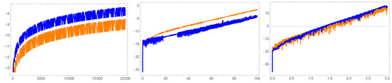
Figure 1. Comparisons of the actual error $E(t,{\xi }_0)$ (orange line) and the geometric numerical test $F(t,q_0)$ (blue line) in natural logarithmic scale. The initial condition is ${\xi }_0=(1,1,100)$. Moreover, the initial conditions in the collective system are $g_{\theta }\ast q_0$ with phase angle $\theta =\{0,{\displaystyle \frac{\pi }{3}},{\displaystyle \frac{2\pi }{3}},\pi ,{\displaystyle \frac{4\pi }{3}},{\displaystyle \frac{5\pi }{3}}\}$. From left to right, each panel corresponds to the systems $X_1$, $X_2$, and $X_3$, respectively.

(a)

The exact solution $s\left(t\right)$ from (A2), (A4), and (A6), depending on the system under consideration, with initial condition ${\xi }_0$;

(b)

The numerical solutions $\tilde{s}\left(t\right)$ of system (17) with the same ${\xi }_0$;

(c)

Several collective solutions ${\tilde{S}}_i\left(t\right)$ of systems (A3), (A5), and (A7) initialized at $g_{\theta }\ast q_0$ and lying on the same orbit.

We plot both the true error $E(t,{\xi }_0)=\parallel s\left(t\right)-\tilde{s}\left(t\right)\parallel$ and the structure-preservation metric $F(t,q_0)$ defined in (2) using logarithmic scaling. Each panel in Figure 1 corresponds to one of the linear systems: the left, center, and right plots depict results for $X_1$, $X_2$, and $X_3$, respectively. Figure 1 reveals that $F(t,q_0)$ tracks $E(t,{\xi }_0)$ with remarkable fidelity, exhibiting an approximately constant vertical offset. This demonstrates that $F(t,q_0)$ reliably quantifies the numerical precision loss during propagation, providing a practical diagnostic tool for geometric structure violation.

4.1.2. Example II: The Free Rigid Body

The free rigid body (FRB) system is completely integrable. The integrals are given by the conservation of the energy $\mathcal{H}$ and the angular momentum $\Pi$:

$$\begin{array}{c}\begin{array}{c}\hfill \mathcal{H}={\displaystyle \frac{1}{2}}\left({\displaystyle \frac{{\Pi }_1^2}{I_1}}+{\displaystyle \frac{{\Pi }_2^2}{I_2}}+{\displaystyle \frac{{\Pi }_3^2}{I_3}}\right),\Pi ={\displaystyle \frac{1}{2}}\left({\Pi }_1^2+{\Pi }_2^2+{\Pi }_3^2\right),\end{array}\end{array}$$

(18)

where $I_i$ are the principal moments of inertia. Hence, the equations of motion are given as

$${\Pi }_1^{\prime }=a_1{\Pi }_2{\Pi }_3,{\Pi }_2^{\prime }=a_2{\Pi }_1{\Pi }_3,{\Pi }_3^{\prime }=a_3{\Pi }_1{\Pi }_2,$$

where $a_1=\left(I_2-I_3\right)/\left(I_2{I}_3\right),a_2=\left(I_3-I_1\right)/\left(I_1{I}_3\right),a_3=\left(I_1-I_2\right)/\left(I_1{I}_2\right)$. Moreover, the equation of motion for the collective FRB system is readily obtained as a standard Hamiltonian system with two degrees of freedom, and Hamiltonian function

$$\tilde{\mathcal{H}}={\displaystyle \frac{1}{2}}\left({\displaystyle \frac{4{(q_3{q}_1-q_4{q}_2)}^2}{I_1}}+{\displaystyle \frac{4{(q_3{q}_4+q_1{q}_2)}^2}{I_2}}+{\displaystyle \frac{{\left(q_3^2-q_4^2-q_1^2+q_2^2\right)}^2}{I_3}}\right).$$

We provide the general solution of the FRB system following [21]. For this purpose, we define the alternative integrals

$$h_1=a_2{\Pi }_3^2-a_3{\Pi }_2^2,h_2=a_3{\Pi }_1^2-a_1{\Pi }_3^2,h_3=a_1{\Pi }_2^2-a_2{\Pi }_1^2.$$

(19)

Once the value of $h_i$ is fixed by the initial condition ${\Pi }^0=({\Pi }_1^0,{\Pi }_2^0,{\Pi }_3^0)$, we consider the following point belonging to the solution evaluated in a time $s=s_0$, which we will employ as the redefinition of the initial condition

$${\Pi }_1\left(s_0\right)={\Pi }_1^0=\sqrt{{\displaystyle \frac{h_3}{a_2}}},{\Pi }_2\left(s_0\right)={\Pi }_2^0=0,{\Pi }_3\left(s_0\right)={\Pi }_3^0=\sqrt{{\displaystyle \frac{h_1}{a_2}}}.$$

Then, we express the general solution in either two forms:

$$\begin{array}{c}\begin{array}{cc}\hfill & {\Pi }_1(s+s_0)=\phantom{-}\sqrt{\left|{\displaystyle \frac{h_3}{a_2}}\right|}\mathrm{cn}({\mu }_{1}s,k_{31}),{\Pi }_1(s+s_0)=\phantom{-}\sqrt{\left|{\displaystyle \frac{h_3}{a_2}}\right|}\mathrm{dn}({\mu }_{3}s,k_{13}),\phantom{ww}\hfill \\ & {\Pi }_2(s+s_0)=-\sqrt{\left|{\displaystyle \frac{h_3}{a_1}}\right|}\mathrm{sn}({\mu }_{1}s,k_{31}),{\Pi }_2(s+s_0)=-\sqrt{\left|{\displaystyle \frac{h_1}{a_3}}\right|}\mathrm{sn}({\mu }_{3}s,k_{13}),\phantom{ww}\hfill \\ & {\Pi }_3(s+s_0)=\phantom{-}\sqrt{\left|{\displaystyle \frac{h_1}{a_2}}\right|}\mathrm{dn}({\mu }_{1}s,k_{31}),{\Pi }_3(s+s_0)=\phantom{-}\sqrt{\left|{\displaystyle \frac{h_1}{a_2}}\right|}\mathrm{cn}({\mu }_{3}s,k_{13}),\phantom{ww}\hfill \end{array}\end{array}$$

(20)

where the elliptic modulus is given by

$$k_{ij}=\sqrt{\left|{\displaystyle \frac{a_i{h}_i}{a_j{h}_j}}\right|},{\mu }_i=\sqrt{|a_i{h}_i|}$$

and $k_{31}\in (0,1)$ iff $a_2{h}_2>0$; for the case $a_2{h}_2<0$, we have that $k_{13}\in (0,1)$.

Figure 2 presents a representative example from our numerical experiments. The plot demonstrates an excellent agreement between the actual error and the geometric numerical test. While different parameter values and initial conditions may introduce a constant vertical offset in some cases, the overall correspondence remains consistently strong across all tested configurations.

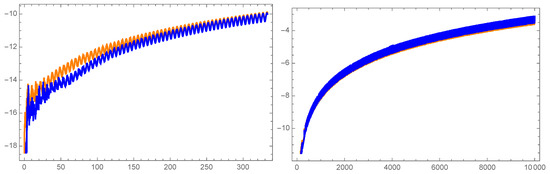
Figure 2. Comparisons of the actual error $E(t,{\Pi }_0)$ (orange line) and the geometric numerical test (blue line) $F(t,q_0)$ given in (2). Initial condition is ${\Pi }_0=(cos(11/10),0,sin(11/10))$. The geometric test is executed for four initial conditions in the collective system given by $q_0^i=g_{{\theta }_i}\ast q_0$ with phase angles ${\theta }_0=0$, ${\theta }_1=\pi /2$, ${\theta }_2=\pi /3$, and ${\theta }_3=5\pi /3$. From left to right, we propagate the numerical evaluations in the intervals $[0,325]$ and $[0,10.000]$, respectively.

As the free rigid body (FRB) system is completely integrable, its first integrals fully constrain the solution trajectories. Consequently, monitoring the conservation of these integrals provides a rigorous test for trajectory deviations in numerical simulations—a well-established diagnostic tool in Hamiltonian dynamics. Figure 3 displays the evolution of both energy and Casimir invariants during numerical integration. Notably, while these traditional invariants fail to capture the solution’s progressive degradation, the proposed geometric test closely tracks the true numerical error throughout the simulation.

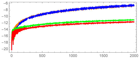
Figure 3. Comparison of the true numerical error $E(t,{\Pi }_0)$ (orange), geometric test $F(t,q_0)$ (blue), energy conservation (red), and Casimir invariant (green). Initial condition ${\Pi }_0=(cos(11/10),0,sin(11/10))$ with four collective initializations $q_0^i=g_{{\theta }_i}\ast q_0$ (${\theta }_i\in \{0,\pi /2,\pi /3,5\pi /3\}$). While the geometric test closely tracks the error evolution across the time interval $[0,2000]$, the traditional conserved quantities (energy and Casimir) remain insensitive to the numerical degradation.

Parameters are chosen to define a triaxial structure to ensure rich dynamics. The initial condition is near an unstable equilibrium, placing the system in a sensitive regime where numerical errors are amplified for clear quantification.

4.2. Geometric Numerical Test in Orbital Dynamics

Celestial mechanics have two fundamental integrable problems: the free rigid body and the Kepler system. We analyzed the first one in the previous section. Here, we consider the case of the unperturbed Kepler system and a perturbation breaking all the associated symmetries.

4.2.1. The Kepler System

It is well known that the Kepler system is maximally super-integrable with an associated Hamiltonian function given by

$${\mathcal{H}}_K={\displaystyle \frac{1}{2}}\left(p_x^2+p_y^2+p_z^2\right)-{\displaystyle \frac{\gamma }{\sqrt{x^2+y^2+z^2}}},$$

where we choose $\gamma =1$ without loss of generality. Besides the energy conservation, we will consider other integrals of motion, such as the angular momentum.

The symmetries of the Kepler system endow the phase space with a fiber bundle structure, and no collective system is needed to be assigned. In order to generate our geometric numerical test, we only need to keep track of the conservation of the fiber bundle structure associated with the G-symmetry. Our experiments consider the diagonal action of $G=SO\left(3\right)$ on the phase space. Thus, the gauge in (2) is given by $g_{\theta }=R(\theta ,\overrightarrow{v})\in SO\left(3\right)$, where $\theta$ and $\overrightarrow{v}$ are the angle and axis of the rotation.

Next, we compare our approach with the classical conservation of the energy and the components of the angular momentum, which are the integrals associated with the $SO\left(3\right)$-symmetry. Precisely, in Figure 4, we plot the energy variation, the conservation of the angular momentum vector modulus, and the geometric numerical test, which measures the conservation of the separation between two solutions of the Kepler system with initial conditions

$$I{C}_1=\{20,-10,-100,3/2000,-3/2000,3/2000\},I{C}_2=R\left({\displaystyle \frac{\pi }{3}},(1,1,1)\right)·I{C}_1.$$

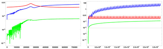
Figure 4. Comparisons of the energy variation (red line), modulus of the angular momentum vector (green line), and the geometric numerical test (blue line). From left to right, we considered 1 and 50 orbital periods, respectively. The initial condition is given by $\{{\xi }_0,y_0,z_0,{p_x}_0,{p_y}_0,{p_z}_0\}=\{20,-10,-100,3/2000,-3/2000,3/2000\}$ and the rotation angle is $\theta =\pi /3$.

In Figure 4 right, we simulate one orbital period, which shows a peak at the passage through the periapsis. The left figure simulates fifty orbital periods, where we observe a deviation in the geometric numerical test and the modulus of the angular momentum. At the same time, the energy remains unaltered, except for the periodic passage through the periapsis. This feature shows that the path described by the particle may be correct, but the position for each time is not. Otherwise, the separation of the initial conditions should be preserved. Notice that only the geometric test has the sensibility to reflect the secular separation between both solutions and their periodic passages through the periapsis. Moreover, the simulation degradation becomes clear for fifty orbital periods, as Figure 5 shows, where the configuration and momenta trajectories become thicker as they go through the periapsis.

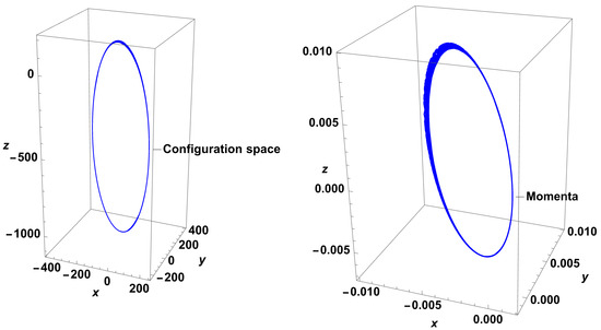
Figure 5. From left to right, we plot the positions and momenta for 50 orbital periods with initial condition $\{{\xi }_0,y_0,z_0,{p_x}_0,{p_y}_0,{p_z}_0\}=\{20,-10,-100,3/2000,-3/2000,3/2000\}$.

4.2.2. Perturbed Kepler System

In most common applications, Keplerian systems are endowed with perturbations destroying all the symmetries. In this case, the only possible test is the conservation of the energy unless we construct the collective system associated with the perturbed Keplerian system. Then, we also have the geometric numerical test proposed in this paper.

In this part, we consider the following perturbed Kepler Hamiltonian:

$$\mathcal{H}={\mathcal{H}}_K+ϵ\mathcal{P},$$

where the perturbation is given by

$$\begin{array}{c}\begin{array}{cc}\hfill \mathcal{P}=& -\omega (x{p}_y-y{p}_x)+b_1{x}^2+b_2{y}^2+b_3{z}^2+c_{1}xy+c_{2}xz+c_{3}yz+axyz.\hfill \end{array}\end{array}$$

(21)

Depending on the values of the parameters $\omega ,b_1,b_2,b_3,c_1,c_2,c_3,a\in \mathbb{R}$, we may obtain several well-known models (Stark, Zeeman, Lunar problem, artificial satellite, galactic tidal effects, etc.).

The collective system associated with this perturbed Keplerian family is again a Hamiltonian system defined in the cotangent bundle $T^{\ast }{\mathbb{R}}_0^4$, which we compute following Section 3.2. Precisely, it is given as the following perturbed harmonic oscillator in resonance 1:1:1:1, which matches the $KS$-regularization of the original Keplerian system:

$$\tilde{\mathcal{H}}={\mathcal{H}}_0+ϵ\tilde{\mathcal{P}},$$

where

$$\begin{array}{c}\begin{array}{cc}\hfill {\mathcal{H}}_0=& {\displaystyle \frac{1}{2}}\left(p_1^2+p_2^2+p_3^2+p_4^2+q_1^2+q_2^2+q_3^2+q_4^2\right),\hfill \\ \hfill \tilde{\mathcal{P}}=& 4\omega (rd-\delta p)+4M\left(4b_1{q}^2+4b_2{p}^2+b_3{m}^2+4c_{1}pq+2c_{2}mq+2c_{3}mp+4dmpq\right),\hfill \end{array}\end{array}$$

(22)

where $\mathbf{v}=(q_1,q_4)$, $\mathbf{w}=(q_2,q_3)$, $\mathbf{V}=(p_4,p_1)$, $\mathbf{W}=(p_3,p_2)$, and we introduce the following notation: $q=det[\mathbf{w},\mathbf{v}]$, $\delta =det[\mathbf{V},\mathbf{w}]+det[\mathbf{W},\mathbf{v}]$, $p=\mathbf{v}·\mathbf{w}$, $r=\mathbf{V}·\mathbf{v}+\mathbf{W}·\mathbf{w}$, $M={\parallel \mathbf{v}\parallel }^2+{\parallel \mathbf{w}\parallel }^2$, $\mu ={\parallel \mathbf{V}\parallel }^2+{\parallel \mathbf{W}\parallel }^2$, and $m={\parallel \mathbf{v}\parallel }^2-{\parallel \mathbf{w}\parallel }^2$.

The collective Hamiltonian $\tilde{\mathcal{H}}$ is endowed with the $S^1$-symmetry given by the action of the Hamiltonian flow associated to $\Xi =q_1{p}_4-p_1{q}_4+q_2{p}_3-p_2{q}_3$. Hence, the gauge $g_{\theta }$ employed in our simulations is given by the diagonal multiplication along the configuration and momenta spaces of the following matrix:

$$g_{\theta }=\left[\begin{array}{cccc}cos\theta & 0& 0& -sin\theta \\ 0& cos\theta & -sin\theta & 0\\ 0& sin\theta & cos\theta & 0\\ sin\theta & 0& 0& cos\theta \end{array}\right]$$

In our simulations, we consider the following values for the parameters:

$$\omega =b_1=b_2=1,b_3=31.3872,c_1=c_3=0,c_2=46.1969,d=-1429.57,ϵ=0.01.$$

These values were specifically tuned to obtain solutions for the non-linear equations involved. With these values, we could compute a $2\pi$-periodic orbit using the sub-harmonic Melnikov method. Precisely, the periodic orbit has initial conditions close to the following point in phase space:

$$(q_0,p_0)=\left({\displaystyle \frac{1}{40}}\left(-\sqrt{3}-1\right),0,{\displaystyle \frac{1}{4\sqrt{2}}},{\displaystyle \frac{\sqrt{3}}{8}},{\displaystyle \frac{1}{40}}\left(\sqrt{3}-1\right),-{\displaystyle \frac{1}{10\sqrt{2}}},{\displaystyle \frac{1}{4\sqrt{2}}},{\displaystyle \frac{1}{8}}\right).$$

A low-eccentricity orbit provides an astrodynamically relevant test case, offering a precise benchmark for evaluating long-term performance and phase-error detection.

First, we consider the original Hamiltonian system given by (21), and we simulated the above-mentioned periodic orbit until we observed that the numeric solution is no longer close to periodic behavior. In Figure 6, we show a numeric simulation of the descended flow for 1, 40, and 101 orbital periods. Notice that the numerical simulation is progressively worsening until it diverges after completing the orbital period 101.

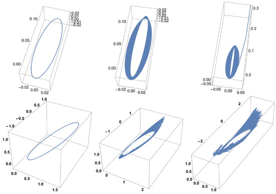
Figure 6. From left to right, we plot 1, 40, and 101 orbital periods of the periodic orbit associated with the perturbed Kepler system (21). The first row corresponds with the configuration space, and the second with the momenta.

Now, we consider the collective Hamiltonian system given by (22). Next, we compare the conservation of the energy, the integral $\Xi$, and the geometric numerical test. Figure 7 shows no significative differences for fewer than five orbital periods. However, after completing the five orbital periods, the geometric numerical test changes tendency with sustained growth, while the energy and the integral $\Xi$ remain almost constant. The images for 10 and 30 orbital periods show that the geometric numerical test detects how the errors are growing, in consonance with the simulations in the descended system given in Figure 6. Only after 101 orbital periods do energy and the integral $\Xi$ suddenly detect the anomalous behavior of the integration.

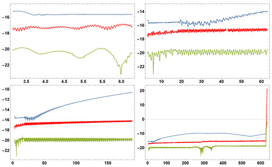
Figure 7. From left to right, we plot 1, 10, 30, and 101 orbital periods of the periodic orbit associated with the collective perturbed Kepler system (22). Gauge computed with $\theta =\pi /3$. Comparisons of the energy variation (red line), Casimir invariant (green line), and the geometric numerical test (blue line) are shown.

5. Conclusions and Future Work

This paper has introduced a novel geometric numerical test designed to evaluate the reliability of numerical simulations by monitoring the preservation of the fiber bundle structure inherent in a system’s phase space.

The efficacy of the proposed geometric test was demonstrated through extensive numerical experiments on both linear and nonlinear systems, including the free rigid body and perturbed Keplerian problems. In all cases, the test $F(t,q_0)$ proved to be a highly sensitive and reliable indicator of numerical error, often detecting precision loss and structural violations much earlier and more clearly than the conservation of classical invariants like energy or angular momentum. This confirms that preserving the underlying geometric structure is a more stringent and informative condition for numerical accuracy than the conservation of first integrals alone.

While this work establishes a framework for geometric numerical testing, several promising directions remain for future research: a comprehensive comparative analysis between our geometric test and established global error estimators (e.g., step-doubling methods). In addition, a direct, quantitative comparison of our geometric test’s performance on benchmark geometric integrators (e.g., variational/symplectic) versus classical methods is mandatory. Moreover, the method should be tested on a wider range of problems to further validate its generality and utility.

Appendix A.1. System X₁

The exact solution of the first system is

$$x\left(t\right)=cos{\displaystyle \frac{t}{2}}-sin{\displaystyle \frac{t}{2}},y\left(t\right)=cos{\displaystyle \frac{t}{2}},z\left(t\right)=100e^{-t}.$$

(A2)

The corresponding collective system on ${\mathbb{R}}_0^4$ is

$$\begin{array}{cc}\hfill {\dot{q}}_1& =0,\hfill \\ \hfill {\dot{q}}_2& ={\displaystyle \frac{-1}{2M{v}^3}}\left(q^{2}p+2p(p^2+v^4)+q(2p^2+2v^4-v^2{w}^2)\right),\hfill \\ \hfill {\dot{q}}_3& ={\displaystyle \frac{-1}{2M{v}^3}}\left(q(q^2+2dp+2p^2+v^4)+p{v}^2{w}^2\right),\hfill \\ \hfill {\dot{q}}_4& ={\displaystyle \frac{1}{2Mv}}\left(q^2+dp-p^2-v^4+v^2{w}^2\right).\hfill \end{array}$$

(A3)

Appendix A.2. System X₂

The exact solution for the second system is

$$x\left(t\right)=e^{0.1t}cos\left(20t\right),y\left(t\right)=e^{0.1t}sin\left(20t\right),z\left(t\right)=e^{-t}.$$

(A4)

The associated collective system in ${\mathbb{R}}_0^4$ reads as follows:

$$\begin{array}{cc}\hfill {\dot{q}}_1& =0,\hfill \\ \hfill {\dot{q}}_2& ={\displaystyle \frac{-1}{10M{v}^3}}\left(200q^{2}p+200p(p^2+v^4)+q\left(6v^4-5v^2{w}^2\right)\right),\hfill \\ \hfill {\dot{q}}_3& ={\displaystyle \frac{-1}{10M{v}^3}}\left(200q^3+200q(p^2+v^4)+p{v}^2(5w^2-6v^2)\right),\hfill \\ \hfill {\dot{q}}_4& ={\displaystyle \frac{1}{10Mv}}\left(q^2+p^2-5v^4+5v^2{w}^2\right).\hfill \end{array}$$

(A5)

Appendix A.3. System X₃

The exact solution to the third system is

$$\begin{array}{cc}\hfill x\left(t\right)& ={\displaystyle \frac{1}{22}}{e}^{-3\sqrt{11}t}\left(11-3\sqrt{11}+(11+3\sqrt{11})e^{6\sqrt{11}t}\right),\hfill \\ \hfill y\left(t\right)& ={\displaystyle \frac{1}{22}}{e}^{-3\sqrt{11}t}\left(11+3\sqrt{11}+(11-3\sqrt{11})e^{6\sqrt{11}t}\right),\hfill \\ \hfill z\left(t\right)& ={\displaystyle \frac{1}{33}}\left(66-\sqrt{11}{e}^{-3\sqrt{11}t}+\sqrt{11}{e}^{3\sqrt{11}t}\right).\hfill \end{array}$$

(A6)

The associated collective system is

$$\begin{array}{cc}\hfill {\dot{q}}_1& =0,\hfill \\ \hfill {\dot{q}}_2& ={\displaystyle \frac{-1}{M{v}^3}}\left(p(q^2+2dp+p^2)+q(q-p)v^2+(10d+p)v^4\right),\hfill \\ \hfill {\dot{q}}_3& ={\displaystyle \frac{-1}{M{v}^3}}\left(q(q^2+2dp+p^2)-(p-q)p{v}^2+(q+10p)v^4\right),\hfill \\ \hfill {\dot{q}}_4& ={\displaystyle \frac{1}{Mv}}\left((q-p)(10(q+p)-v^2)\right).\hfill \end{array}$$

(A7)

References

- Roa, J.; Urrutxua, H.; Peláez, J. Stability and chaos in Kustaanheimo–Stiefel space induced by the Hopf fibration. Mon. Not. R. Astron. Soc. 2016, 459, 2444–2454. [Google Scholar] [CrossRef]
- Valle, S.C.D.; Urrutxua, H.; Solano-López, P. Exploiting Gauge Freedom in KS Variables for High-Performance Numerical Orbital Propagation. In Proceedings of the Proceedings of the International Astronautical Congress (IAC), Milan, Italy, 14–18 October 2024; pp. 1537–1552. [Google Scholar] [CrossRef]
- van der Meer, J. The Kepler system as a reduced 4D harmonic oscillator. J. Geom. Phys. 2015, 92, 181–193. [Google Scholar] [CrossRef]
- Ferrer, S.; Crespo, F. Alternative Angle-Based Approach to the KS-Map. An Interpretation Through Symmetry and Reduction. J. Geom. Mech. 2018, 10, 359–372. [Google Scholar] [CrossRef]
- Crespo, F.; Ferrer, S. Alternative Reduction by Stages of Keplerian Systems. Positive, Negative, and Zero Energy. Siam J. Appl. Dyn. Syst. 2020, 19, 1525–1539. [Google Scholar] [CrossRef]
- McLachlan, R.I.; Modin, K.; Verdier, O. Collective Lie–Poisson integrators on R3. Ima J. Numer. Anal. 2014, 35, 546–560. [Google Scholar] [CrossRef]
- McLachlan, R.I.; Modin, K.; Verdier, O. Collective symplectic integrators. Nonlinearity 2014, 27, 1525. [Google Scholar] [CrossRef]
- MuntheKaas, H. Geometric integration on symmetric spaces. J. Comput. Dyn. 2024, 11, 43–58. [Google Scholar] [CrossRef]
- Hairer, E.; Wanner, G.; Lubich, C. Geometric Numerical Integration. Structure-Preserving Algorithms for Ordinary Differential Equations, 2nd ed.; Springer: Berlin/Heidelberg, Germany, 2006. [Google Scholar]
- Leimkuhler, B.; Reich, S. Simulating Hamiltonian Dynamics; Cambridge University Press: Cambridge, UK, 2004. [Google Scholar]
- Sanz-Serna, J.M. Numerical Hamiltonian Problems; Courier Dover Publications: Mineola, NY, USA, 2018. [Google Scholar]
- Nakahara, M. Geometry, Topology and Physics, 2nd ed.; Institute of Physics Publishing: Bristol, UK, 2003. [Google Scholar]
- Lee, J. Introduction to Smooth Manifolds, 2nd ed.; Graduate Texts in Mathematics; Springer: Berlin/Heidelberg, Germany, 2012; Volume 218. [Google Scholar] [CrossRef]
- Meyer, K. Symmetries and Integrals in Mechanics. Dynamical Systems; Academic Press: Cambridge, MA, USA, 1973; pp. 259–272. [Google Scholar] [CrossRef]
- Marsden, J.; Weinstein, A. Reduction of symplectic manifolds with symmetry. Rep. Math. Phys. 1974, 121–130. [Google Scholar] [CrossRef]
- Hilbert, D. Ueber die Theorie der algebraischen Formen. Math. Ann. 1890, 36, 473–534. [Google Scholar] [CrossRef]
- Weyl, H. The Classical Groups, Their Invariants and Representations; Princenton Univ. Press: Princeton, NJ, USA, 1946. [Google Scholar]
- Schwarz, G. Smooth function invariant under the action of a compact Lie group. Topology 1975, 14, 45–64. [Google Scholar] [CrossRef]
- Poenaru, V. Singularités C∞ en Présence de Symétrie; LNM; Springer: Berlin/Heidelberg, Germany, 1976; Volume 510. [Google Scholar]
- Saha, P. Interpreting the Kustaanheimo-Stiefel transform in gravitational dynamics. Mon. Not. R. Astron. Soc. 2009, 400, 228–231. [Google Scholar] [CrossRef]
- Crespo, F.; Ferrer, S. On the extended Euler system and the Jacobi and Weierstrass elliptic functions. J. Geom. Mech. 2015, 7, 151–168. [Google Scholar] [CrossRef]
- Ortega, J.P.; Ratiu, T.S. Momentum Maps and Hamiltonian Reduction; Birkhauser: Boston, MA, USA, 2004. [Google Scholar]
- Bluman, G.W.K.S. Symmetries and Differential Equations; Springer: New York, NY, USA, 1989. [Google Scholar]
- Olver, P.J. Applications of Lie Groups to Differential Equations, 2nd ed.; Springer: New York, NY, USA, 1993. [Google Scholar]
- Marsden, J.; Ratiu, T. Introduction to Mechanics and Symmetry, 2nd ed.; Texts in Applied Mathematics; Springer: New York, NY, USA, 1999; Volume 17. [Google Scholar]
Disclaimer/Publisher’s Note: The statements, opinions and data contained in all publications are solely those of the individual author(s) and contributor(s) and not of MDPI and/or the editor(s). MDPI and/or the editor(s) disclaim responsibility for any injury to people or property resulting from any ideas, methods, instructions or products referred to in the content. |
© 2025 by the authors. Licensee MDPI, Basel, Switzerland. This article is an open access article distributed under the terms and conditions of the Creative Commons Attribution (CC BY) license (https://creativecommons.org/licenses/by/4.0/).