Optimization of Multi-Vehicle Cold Chain Logistics Distribution Paths Considering Traffic Congestion

Abstract

Urban road traffic congestion has become a serious issue for cold chain logistics in terms of delivery time, distribution cost, product freshness, and even organization revenue and reputation. This study focuses on the cold chain distribution path by considering road traffic congestion with transportation, real-time vehicle delivery speeds, and multiple-vehicle conditions. Therefore, a vehicle routing optimization model has been established with the objectives of minimizing costs, reducing carbon emissions, and maintaining cargo freshness, and a multi-objective hybrid genetic algorithm has been developed in combination with large neighborhood search (LNSNSGA-III) for leveraging strong local search capabilities, optimizing delivery routes, and enhancing delivery efficiency. Moreover, by reasonably adjusting departure times, product freshness can be effectively enhanced. The vehicle combination strategy performs well across multiple indicators, particularly the three-type vehicle strategy. The results show that costs and carbon emissions are influenced by environmental and refrigeration temperature factors, providing a theoretical basis for cold chain management. This study highlights the harmonious optimization of cold chain coordination, balancing multiple constraints, ensuring efficient logistic system operation, and maintaining equilibrium across all dimensions, all of which reflect the concept of symmetry. In practice, these research findings can be applied to urban traffic management, delivery optimization, and cold chain logistics control to improve delivery efficiency, minimize operational costs, reduce carbon emissions, and enhance corporate competitiveness and customer satisfaction. Future research should focus on integrating complex traffic and real-time data to enhance algorithm adaptability and explore customized delivery strategies, thereby achieving more efficient and environmentally friendly logistics solutions.

1. Introduction

Urban road conditions have become increasingly complex, with traffic congestion emerging as a significant factor affecting supply chain efficiency. Richard [1] contends that traffic congestion has become one of the “plagues” of modern city life in large cities because it restricts the travel speed of cold chain logistics delivery vehicles; it not only affects vehicle fuel consumption, increases delivery costs and carbon emissions, but also reduces the freshness of goods upon arrival, ultimately leading to revenue loss and reputational damage for enterprises.

To address this phenomenon, many scholars and experts have focused their research on road traffic congestion, exploring various delivery strategies or modes to mitigate the losses incurred by enterprises due to traffic congestion. However, the academic community has relatively weak quantitative standards to assess traffic congestion. In existing academic research related to vehicle route optimization, most scholars have set the traffic congestion coefficients (TCC) simply as overall traffic congestion coefficients (OTCC) based on the road traffic condition in the service area and conducted related research. However, cities generally have multiple administrative regions, and the service areas of enterprises often encompass multiple administrative regions. When enterprises dispatch vehicles to perform delivery tasks, because the customers in the orders are located in different administrative regions, vehicles frequently need to cross multiple administrative regions during the delivery process. Based on actual conditions, the average road traffic congestion coefficients in different administrative regions usually vary during the same time period; therefore, when a vehicle transfers from one administrative region to another within a certain time frame, influenced by TCC, the driving speed of the delivery vehicle will change significantly, which in turn affects vehicle fuel consumption and the delivery time of goods. Therefore, this paper argues that when an enterprise’s delivery service needs to span regions, considering the traffic congestion coefficients by subregion (TCC-S) may be more appropriate and yield more reliable and practical route planning for enterprises.

This study aims to address the challenges of cold chain logistics under traffic congestion conditions by establishing a multi-objective vehicle routing optimization model considering cross-regional traffic congestion coefficients and multiple vehicle models and employing a hybrid metaheuristic algorithm to achieve a balanced optimization of cost, carbon emissions, and cargo freshness, thereby improving logistics efficiency and sustainability. Specifically, this paper focuses on cold chain logistics transportation, centering on the vehicle routing problem across regions (CRDVRP), quantifying the real-time delivery speed of cold chain logistics vehicles during the delivery process, and also considering the conditions of multiple vehicle models. A vehicle routing optimization model is established with the objectives of minimizing the costs of carbon emissions and maintaining the average cargo freshness upon arrival at the customer’s location, and corresponding research is conducted. This problem is NP-hard, meaning that it is difficult to obtain an optimal solution within a limited time. Therefore, a hybrid metaheuristic algorithm is developed by combining the third-generation non-dominated sorting genetic algorithm and the large neighborhood search algorithm to find near-optimal solutions to the problem. In summary, the work and innovations of this paper are as follows:

(1)

Traffic Congestion Coefficient and Vehicle Speed Model: In this paper, we collect traffic congestion coefficients from various administrative regions within a company’s delivery area over several months. Through numerical fitting techniques, we derive traffic congestion coefficients for each region across a 24 h period. Based on these coefficients, we construct a model to calculate vehicle speeds. Building on this foundation, we develop a multi-objective mixed-integer nonlinear programming model that incorporates cost, carbon emissions, and cargo freshness. This model ensures a symmetrical balance among these different objectives, aiming for a reasonable allocation and optimal configuration of cost, environmental impact, and product quality.

(2)

Proposal for the LNSNSGA-III Algorithm: This paper presents a multi-objective hybrid genetic algorithm incorporating Large Neighborhood Search (LNS) with NSGA-III, termed LNSNSGA-III. By combining the local search prowess of the LNS with the global search efficiency of NSGA-III, this algorithm effectively mitigates the risk of premature convergence. The LNSNSGA-III algorithm not only augments the robustness and diversity of feasible solutions but also assimilates the principle of symmetry into the multi-objective optimization framework. This approach ensures a harmonious balance across various objectives and markedly enhances the overall optimization efficacy of the delivery system.

The remainder of this paper is structured as follows. Section 2 introduces the current state of related research. Section 3 describes the research problem, introduces the calculation method for vehicle travel speeds considering TCF-S, and presents the calculation methods for the cost function, carbon emission function, and freshness function, further establishing a multi-objective mixed-integer nonlinear programming model. Section 4 introduces LNSNSGA-III. Section 5 evaluates the algorithm using benchmark instances and analyzes the model’s sensitivity to different parameter settings. Section 6 presents the research conclusions and future outlook.

2. Literature Review

With the rapid development of globalization and e-commerce, the process of urbanization has accelerated, leading to a sharp increase in the number of urban populations and vehicles. This, in turn, has exacerbated urban traffic congestion issues. Traffic congestion not only reduces the efficiency of logistics and increases delivery costs, but also has negative environmental impacts. According to data from the World Bank, over 50% of the global population lives in urban areas, where traffic congestion is increasingly severe. Congestion leads to decreased vehicle speed, increased fuel consumption and emissions, and prolonged delivery times. During peak hours, congestion is particularly severe, causing delivery vehicles to take several times longer to complete their tasks. For example, in major cities like New York and Beijing, traffic congestion has become a bottleneck for urban development, with average vehicle speeds during peak hours dropping to 10–20 km per hour, far below normal driving speeds. Jin [2] analyzed data from 86 metropolitan areas using a simultaneous equation model and found that the growth of traffic congestion has a negative economic impact, which varies across different stages of economic prosperity and recession.

To address traffic congestion, Anthony [3] proposed a vehicle routing optimization problem to tackle peak-hour traffic congestion. Li [4] developed a dynamic road network model based on graph theory and time-varying traffic data, incorporating a road impedance model. Niu [5] designed variable speed limits under different levels of congestion and adverse weather conditions, defining parameters for highways. The study found that reasonable speed limits can effectively reduce road delays and improve operational efficiency in certain traffic areas; however, inappropriate speed limits at low traffic volumes can significantly inhibit highway efficiency. Daniel [6] found that vehicle density and congestion have implications for road investment and regional productivity growth. Ming [7] discovered that current regional traffic congestion coordination control methods do not consider the impact of key links, and thus proposed a regionally coordinated traffic congestion control method based on critical links. Regarding the CRDVRP, Carlsson [8] experimentally demonstrated the efficiency of the proposed regional partition strategy using synthetic and real datasets. You [9] established an energy dissipation model considering road gradients, traffic flows, and congestion and proposed an efficient vehicle routing algorithm for sustainable transportation.

Traffic congestion significantly affects vehicle speed. In the current state of research on vehicle speeds under congestion conditions, Zhang [10] developed a new fuel consumption model considering vehicle speed and acceleration, creating a novel model for calculating speed fluctuation states. David [11] established a vehicle speed curve that minimizes work and fuel consumption while also reducing fuel consumption in land transport vehicles (road or rail) traversing paths or routes. In the context of green transport scheduling with speed control, Salehi [12] proposed a new transport scheduling and driver assignment model by balancing total transport costs and carbon emissions. Liu [13] studied the green vehicle routing problem with dynamic driving speeds from both temporal and spatial dimensions. Wang [14] constructed a transient speed model describing vehicle speed and road traffic flow changes by simulating urban traffic flows and established a vehicle routing problem model considering traffic.

Goyal [15] investigated real-time carbon emissions under traffic congestion conditions and found a relationship between carbon emissions and vehicle speed. This is because traffic congestion leads to repeated operations such as ‘starting’, ‘accelerating’, ‘braking’, and ‘idling’, which increase fuel consumption and carbon emissions in congested conditions. In research related to carbon emissions in VRP, Ahmed [16] designed a mixed-integer linear programming model with the dual objectives of minimizing costs and carbon emissions to address the issue of excessive carbon emissions in cold chain logistics. Mohammad [17] studied multi-objective supply chain scheduling considering carbon emissions, using two functions to calculate emissions during empty and full-load transport. Xu [18] calculated carbon emissions using automotive fuel consumption and designed a mixed-integer nonlinear programming model with the dual objectives of minimizing fuel consumption and maximizing customer satisfaction. Gao [19] examined the correlation between carbon emissions, vehicle fuel consumption, and highway congestion, finding that higher congestion levels on highways result in greater carbon emissions.

Regarding the Multi-Depot Vehicle Routing Problem (MDVRP), Li [20] studied a new multi-vehicle routing problem model with time windows, proposing a strategy that allows flexible stop selection and establishing an integer programming model to minimize total travel costs. Sundar [21] addressed the Multiple Depot, Fuel-Constrained, Multiple Vehicle Routing Problem (FCMVRP) under conditions of multiple depots and fuel constraints, determining the lowest total cost for each vehicle’s route while ensuring that each vehicle reaches every target at least once and does not run out of the fuel en route. Fernando [22] introduced a cooperative evolutionary algorithm to minimize the total route cost of MDVRR and proposed an evolutionary strategy with variable-length genotypes and local search operators. Luo [23] developed a new multi-phase improved Shuffled Frog Leaping Algorithm (MPMSFLA) to solve MDVRP, which is suitable for solving large-scale problems. At the same time, Ahmad [24] further improved the model parameters, and the non-dominated sorting mechanism and optimization strategies for reducing environmental disturbances and improving the efficiency of transportation routes are more effective in solving large-scale problems. Regarding the Stochastic MDVRP (SMDVRP), Laura [25] proposed a simulation-heuristic framework combining Monte Carlo simulation and meta-heuristic algorithms to handle the SMDVRP.

Additionally, since fresh food must be transported under low-temperature conditions [26] to maintain the quality and extend the shelf life of transported food, research on cold chain logistics has been significant. Wang [27] in 2016 constructed a multi-objective distribution route optimization model to maximize freshness and minimize total costs, using a two-stage multi-objective algorithm based on Pareto solutions. Accorsi [28] proposed a mixed-integer linear programming model for planning the production, storage, and distribution of perishable products and found that the model significantly reduces transport costs and saves substantial economic and environmental costs for cold chains. Li [29] developed a real-time responsive cold chain distribution scheduling decision model, which also effectively saves costs. Jia [30] explored the current status, challenges, and future trends of fresh produce cold chain logistics. Imran [31] conducted an in-depth study on a comprehensive approach to cold chain logistics risk and resilience.

Based on the research background above, this paper further integrates the concept of “symmetry” into the study, emphasizing balance and harmony in multi-objective optimization and cross-regional delivery problems. Specifically, symmetry will be reflected in the following aspects:

(1)

Multi-Objective Balance: The vehicle routing optimization problem involves conflicting objectives, such as cost, carbon emissions, and cargo freshness. This study constructs a multi-objective optimization model to find a balance among these objectives, which is the core essence of symmetry. This balance not only requires equitable allocation among objectives but also aims to optimize resource allocation across the entire delivery system. Utilizing the LNSNSGA-III algorithm, the paper effectively explores multiple feasible solutions, ensuring equilibrium among cost, emissions, and freshness, thereby enhancing system efficiency.

(2)

Traffic Congestion Coefficient Symmetry: In cross-regional delivery, traffic congestion coefficients (TCC-S) in different administrative regions may vary significantly. By introducing subregional traffic congestion coefficients, this paper ensures symmetry across different regions. This symmetry is reflected in the reasonable adjustment of vehicle speeds, fuel consumption, and delivery times as vehicles move between regions, making the entire delivery process smoother and more balanced. This approach improves the operational efficiency of the delivery system and reduces the uncertainties caused by differences in regional traffic conditions.

(3)

Vehicle Combination and Delivery Path Symmetry: In multi-vehicle-type delivery, different types of vehicles have varying load capacities and fuel consumption characteristics. By designing a reasonable vehicle combination strategy, this paper ensures balanced vehicle allocation across different routes and regions, preventing over-concentration or under-utilization of vehicles in certain areas. This achieves symmetric optimization of vehicle routing. Such symmetry design not only enhances delivery efficiency but also reduces the over-concentration of vehicles across regions, further alleviating traffic congestion.

(4)

Departure Time and Delivery Process Symmetry: In the delivery process, reasonable adjustment of departure times is also key to achieving symmetry. By optimizing departure times, this paper ensures that vehicle tasks in different regions are performed during off-peak hours, avoiding concentrated deliveries during peak traffic congestion times, thereby achieving symmetry in the delivery process. This symmetry is reflected in the balanced distribution of vehicles across different time periods, reducing the impact of traffic congestion on the delivery efficiency of enterprises.

In summary, this paper incorporates the concept of symmetry, not only achieving balance in multi-objective optimization but also reflecting symmetry in regional traffic congestion coefficients, vehicle combination strategies, and departure time adjustments in cross-regional delivery. This symmetry design makes the delivery system more efficient, balanced, and stable, aligning with the expectations of the journal Symmetry regarding the concept of symmetry. Future research will explore ways to further enhance the adaptability and precision of symmetry design through more complex traffic data and real-time information, thereby providing enterprises with more efficient and environmentally friendly logistics solutions.

3. Problem Modeling

3.1. Problem Description

As depicted in Figure 1, the fresh produce distribution center (the Center) receives delivery orders that encompass details such as the coordinates of target customers, their service time windows, and the quantities demanded. The distribution center is tasked with delivering goods to all customer points within their specified service time windows, aiming to minimize both overall delivery costs and carbon emissions, while maximizing the average freshness of the goods upon delivery to all customers. To address this complex problem, a multi-objective optimization mathematical model is established, offering multiple delivery plans for the distribution center to select the most suitable option.

During the delivery period, since the customers within the order are located in different regions, each region has an independent Traffic Congestion Coefficient (TCC), which varies with time. The distribution center has K types of N cold chain logistics transport vehicles, and the average driving speed of different vehicle types K is affected differently by the TCC. The distribution center needs to coordinate different types of delivery vehicles to complete delivery tasks.

3.2. Assumptions

Assumption 1. 

The fresh produce distribution center (Center) has K types of N cold chain logistics transport vehicles that can perform delivery tasks.

Assumption 2. 

The fresh produce distribution center (Center) is located in a city with R administrative regions, each with an independently varying traffic congestion function. The degree of congestion changes with time, and all vehicle speeds are affected by the congestion level.

Assumption 3. 

The distribution service area of the fresh produce distribution center (Center) covers R administrative regions.

Assumption 4. 

The time for vehicle delivery to customer points cannot be earlier than the customer’s time window, but can be later.

Assumption 5. 

The baseline driving speed of vehicles within region R depends on the average driving speed of all vehicles when the roads are not congested.

3.3. Parameter Description

Distribution Center (Center) Identification: 0.

Customer Point Identification (M): {1, 2, …, m}.

Vehicle Identification (N): {1, 2, …, n}.

Vehicle Type Identification (K): {1, 2, 3}.

$m_k\{m_1,m_2,m_3\}$: c

$mt{d}_k=\{mt{d}_1,mt{d}_2,mt{d}_3\}$: Maximum Travel Distance of Vehicle Type k.

$nee{d}_m=\{nee{d}_1,nee{d}_2,\dots ,nee{d}_m\}$: Demand Quantity at Customer Point m.

Vehicle n Travels from Point i to Point j ($x_{\mathrm{i}\mathrm{j}}^n$): 1 if vehicle n travels from i to j; otherwise, it is 0.

Vehicle n is of Type k ($y_n^k$): 1 if vehicle n is of type k, otherwise 0.

$d_{ij}$: Distance traveled by vehicles from i to j.

$R=\{R_1,R_2,\dots ,R_r\}$: Sub-regions within the Delivery Range.

$\overline{V}=\{{\overline{v}}_{R_1},{\overline{v}}_{R_2},\dots ,{\overline{v}}_{R_r}\}$: Average Speed of Vehicles in Sub-region $R_r$ when Congestion Coefficient is 1.

$V_k=\{1.2\overline{V},\overline{ V},0.8\overline{V}\}$: Average Speed of Vehicle Type k in Each Sub-region when Congestion Coefficient is 1.

$t_0^n$: Departure Time of Vehicle n from the Distribution Center.

$t_1^m ,t_2^m ,t_3^m$: Arrival time at point m, start service time at point m, and departure time from point m.

$[t_l^i , t_r^i]$: Required Service Time Window for Customer Point i.

$[I,E]$: Service Time Window for the Distribution Center.

$t_s$: Service Duration at Customer Point.

$c_1^k$: Unit Fixed Cost of Vehicle Type k.

$c_2$: Price per Liter of Fuel.

$c_3$: Cost per Kilogram of Carbon Emission.

$c_4$: Penalty Coefficient for Delivery Delay.

3.4. Vehicle Speed Function Modeling

The Traffic Congestion Coefficient (TCC) is a quantified metric used to measure the degree of traffic congestion, with a range of [1, ∞), representing a spectrum from smooth traffic flow to extreme congestion. The quantification method for TCC in this paper is based on the Baidu Maps Traffic and Travel Big Data Platform [32], as shown in Equation (1).

$$\mathrm{T}\mathrm{C}\mathrm{C}={\displaystyle \frac{t_{ij}^{\prime }}{t_{ij}}}$$

(1)

where $t_{ij}^{\prime }$ represents the actual travel time from point i to point j. $t_{ij}$ represents the traveling time of the vehicle from point i to point j under free flow. Therefore, from Equation (1), the following derivation can be made to obtain Equation (2):

$${\displaystyle \frac{t_{ij}^{\prime }}{t_{ij}}}={\displaystyle \frac{\frac{d_{ij}}{v_{ij}^{\prime }}}{\frac{d_{ij}}{v_{ij}}}}={\displaystyle \frac{v_{ij}}{v_{ij}^{\prime }}}$$

(2)

According to Equation (2), TCC is also the ratio of the vehicle’s average speed under free-flow and non-free-flow conditions. Thus, by combining Equation (1), the average speed of vehicles under non-free-flow conditions is derived, as shown in Equation (3):

$$v_{ij}^{\prime }={\displaystyle \frac{v_{ij}}{\mathrm{T}\mathrm{C}\mathrm{C}}}={\displaystyle \frac{V_k}{\mathrm{T}\mathrm{C}\mathrm{C}}}$$

(3)

Additionally, the relationship between vehicle speed and TCC obtained from Equation (3) is shown in Figure 2, where the vehicle speed decreases with increasing TCC.

According to the Baidu Maps’ Big Data Platform, dividing a day (24 h) into h = 288 equal-length time intervals (5-min intervals), the TCC for each interval is shown in Equation (4), where r represents an administrative region, R represents the service region, $r\in R$, and h represents the time interval.

$${TCC}_h^r=\left\{{TCC}_1^r,{TCC}_2^r,\dots ,{TCC}_{288}^r\right\}$$

(4)

Combining Equations (3) and (4), the average speed of a vehicle of type k in sub-region r during time interval h (assuming that the vehicle is in motion) is derived as shown in Equation (5):

$$v_k^r={\displaystyle \frac{v_k}{\left\{{TCC}_h^r\right\}}}=\{{\displaystyle \frac{V_k}{{TCC}_1^r}},{\displaystyle \frac{V_k}{{TCC}_2^r}},\dots ,{\displaystyle \frac{V_k}{{TCC}_{288}^r}}\}$$

(5)

In this paper, time is uniformly converted to real numbers within $t\in \left[\mathrm{0,24}\right)$. The membership function between time t and the divided h time intervals is

$$h\left(t\right)=fix\left(t\ast 12\right)+1$$

(6)

where $fix\left(\right)$ denotes the operation of rounding down to the nearest integer. Substituting Equation (6) into Equation (5) yields

$$v_k^r\left(t\right)={\displaystyle \frac{V_k}{{TCC}_{h\left(t\right)}^r}}$$

(7)

Equation (7) represents the average traveling speed of a vehicle of type k in sub-region r at time t (assuming that the vehicle is in motion).

3.5. Carbon Emission Function Modelling

Suppose the carbon emissions $P$ considered in this model are composed of carbon emissions $P_1$ generated by refrigerated transport vehicles during normal driving and carbon emissions $P_2$ produced by the fuel consumption of their refrigeration units.

Firstly, as shown in Figure 3, the sub-regions and distances traversed by the vehicle from point i to point j are represented;

The set of sub-regions traversed by the vehicle from point i to point j is defined as in Equation (8):

$$R_{ij}=\left\{r_1,r_2,\dots ,r_n\right\},n\ge 1,{\forall r}_n\in R$$

(8)

Similarly, the set of distances traversed by the vehicle from point i to point j within each sub-region is defined as in Equation (9):

$$L_{ij}=\left\{L_{r_1},L_{r_2},\dots ,L_{r_n}\right\},{\forall r}_n\in R_{ij}$$

(9)

The real-time load of vehicle n from point i to point j is denoted as $g_{ij}^n$, and the ratio of the real-time load to its maximum load is denoted as θ. According to the calculation method of the MEET model in reference [33], combined with this model, the carbon emission rate $w_k$ of vehicle with type k in sub-region r, during time period h, driving unloaded at a speed $v={\displaystyle \frac{V_k}{{TCC}_h^r}}$, and on a slope of 0° is defined as:

$$w_k(\mathrm{v},{\phi }^k)={\phi }_0^{\mathrm{k}}+{\phi }_1^k\mathrm{v}+{\phi }_2^k{\mathrm{v}}^2+{\phi }_3^k{\mathrm{v}}^3+{\displaystyle \frac{{\phi }_4^k}{\mathrm{v}}}+{\displaystyle \frac{{\left({\phi }_5^k\right)}^2}{v}}+{\displaystyle \frac{{{(\phi }_6^k)}^3}{v}}$$

(10)

where ${\phi }^k={\{\phi }_0^k,{\phi }_1^k,{\phi }_2^k,{\phi }_3^k,{\phi }_4^k,{\phi }_5^k,{\phi }_k^k\}$ represents the parameters of the carbon emission rate for vehicle type k. The load correction factor ${\mathrm{\varnothing }}_k$ of the vehicle on the road is defined as in Equation (11):

$${\mathrm{\varnothing }}_k(\mathrm{v},\mathsf{\theta },{\beta }^k)={\beta }_0^{\mathrm{k}}+{\beta }_1^k\theta +{\beta }_2^k{\theta }^2+{\beta }_3^k{\theta }^3+{\beta }_4^k\mathrm{v}+{\beta }_5^k{\mathrm{v}}^2+{\beta }_6^k{\mathrm{v}}^3+{\displaystyle \frac{{\beta }_7^k}{\mathrm{v}}}$$

(11)

where ${{\beta }^k=\{\beta }_0^k,{\beta }_1^k,{\beta }_2^k,{\beta }_3^k,{\beta }_4^k,{\beta }_5^k,{\beta }_6^k,{\beta }_0^k\}$ represents the correction parameters for the load weight of fuel vehicles of type k. Therefore, the carbon emissions $\epsilon (v,\theta ,{{\phi }^k,\beta }^k)$ of vehicle type k in sub-region r during time period h and traveling a distance of dis are defined as in Equation (12):

$$\epsilon \left(v,\theta ,{{\phi }^k,\beta }^k,dis\right)={\displaystyle \frac{w_k\left(\mathrm{v},{\phi }^k\right){\ast \mathrm{\varnothing }}_k\left(\mathrm{v},\mathsf{\theta },{\beta }^k\right)}{1000}}\ast dis$$

(12)

In this model, since the carbon emissions generated by the vehicle traveling from any point to another are not conveniently expressed using standard operations research formulas, we use pseudocode to express the calculation rules. The pseudocode for calculating the carbon emissions $p_{ij}$ generated by vehicle type k from point i to point j during normal driving is shown in

Table 1. Algorithm for carbon emission calculation.

$\mathbf{I}\mathbf{n}\mathbf{p}\mathbf{u}\mathbf{t}$	$\mathit{k},{\mathit{p}}_{\mathit{i}\mathit{j}}=0,{\mathit{\phi }}^{\mathit{k}},{\mathit{\beta }}^{\mathit{k}},\mathbf{n}=\left|{\mathit{R}}_{\mathit{i}\mathit{j}}\right|,{\mathit{t}}_{\mathit{l}}=\frac{5}{60},$ ${\mathit{R}}_{\mathit{i}\mathit{j}},{\mathit{L}}_{\mathit{i}\mathit{j}},\mathit{\theta },\mathit{t}={\mathit{t}}_3^{\mathit{i}}$
1	$\mathrm{f}\mathrm{o}\mathrm{r} \mathrm{i}=1 \mathrm{t}\mathrm{o} \mathrm{n}$
2	$\mathrm{d}\mathrm{i}\mathrm{s}=L_{ij}\left(i\right),\mathrm{r}=R_{ij}\left(i\right)$
3	$\mathrm{W}\mathrm{h}\mathrm{i}\mathrm{l}\mathrm{e} \mathrm{d}\mathrm{i}\mathrm{s}>0$
4	$v=v_k^r\left(t\right)$
5	$di{s}^{\prime }=v\ast t_l$
6	$if dis<di{s}^{\prime }$
7	$t=t+{\displaystyle \frac{dis}{v}}$
8	$oil=oil+\epsilon (v,\theta ,{\phi }^k,{\beta }^k,dis)$
9	$else$
10	$t=t+t_l$
11	$oil=oil+\epsilon (v,\theta ,{\phi }^k,{\beta }^k,di{s}^{\prime })$
12	$dis=dis-di{s}^{\prime }$
13	$end if$
14	$end while$
15	$end for$
$\mathrm{o}\mathrm{u}\mathrm{t}\mathrm{p}\mathrm{u}\mathrm{t}$	$p_{ij} , t_1^j=t$

.

The input end n represents the length of the set, $t_l$ represents the conversion of the time interval of 5 min to length, and t represents the start calculation time (the time at which the vehicle leaves point i). The output results are the carbon emissions $p_{ij}$ from point i to point j and the time $t_1^j$ at which the vehicle arrives at point j. Therefore, during the overall distribution process, the carbon emissions generated by the vehicle-consuming fuel during normal driving are calculated using Equation (13):

$$P_1=\sum _{k=1}^3\sum _{n=1}^N\sum _{j=0}^m\sum _{i=0}^m{p}_{ij}{x}_{ij}^n{y}_n^k,(i\ne j)$$

(13)

According to reference [34], the fuel consumption G of a vehicle n’s refrigeration unit generator can be expressed as

$$G=G_n{g}_{ij}^n{Tr}_{0j}^n={\displaystyle \frac{G_{*}^n-G_0^n}{Q_{max}^n}}{g}_{ij}^n{Tr}_{0j}^n$$

(14)

In Equation (14), ${\mathrm{G}}_{*}^{\mathrm{n}}$ represents the unit time fuel consumption of the generator when vehicle n is fully loaded, ${\mathrm{G}}_0^{\mathrm{n}}$ represents the unit time fuel consumption when vehicle n is empty, ${\mathrm{Q}}_{\mathrm{m}\mathrm{a}\mathrm{x}}^{\mathrm{n}}$ represents the maximum load of vehicle n, ${\mathrm{g}}_{\mathrm{i}\mathrm{j}}^{\mathrm{n}}$ represents the real-time load of vehicle n from point i to point j, ${\mathrm{T}\mathrm{r}}_{0\mathrm{j}}^{\mathrm{n}}$ represents the time difference between vehicle n arriving at point j and leaving the distribution center, and ${\mathrm{G}}_{\mathrm{n}}$ represents the refrigeration fuel consumption coefficient of vehicle n (unit: L/(h ∗ kg)).

Meanwhile, taking the actual situation into account, the higher the external environmental temperature, the greater the power required by the vehicle’s refrigeration generator to maintain the desired refrigeration temperature. Consequently, the coefficient of refrigeration fuel consumption will increase, leading to a corresponding increase in fuel consumption. At this time, the fuel consumption $G^{\prime }$ of vehicle n refrigeration unit generator can be expressed as:

$$G^{\prime }=G_n^{\prime }{g}_{ij}^n{Tr}_{0j}^n=\left\{\begin{array}{c}{G}_n\left(1-\alpha \left(T_{*}-T_0\right)\right)g_{ij}^n{Tr}_{0j}^n , T_{*}<T_0\\ G_n\left(1-\alpha \left(T_0-T_{*}\right)\right)g_{ij}^n{Tr}_{0j}^n , T_{*}>T_0\\ G_n{g}_{ij}^n{Tr}_{0j}^n , T_{*}=T_0\end{array}\right.$$

(15)

In Equation (15), $T_{*}$ represents the refrigeration temperature of the refrigerated truck, $T_0$ represents the average ambient temperature of the day, and $\alpha$ represents the influence parameter of the temperature difference on refrigeration fuel consumption. According to the literature, the ratio of fuel weight to carbon emissions is approximately 2.3; therefore, during the overall distribution process, the carbon emissions generated by the vehicle’s refrigeration generator consuming fuel are calculated using Equation (16):

$$P_2={\sum }_{k=1}^3{\sum }_{n=1}^N{\sum }_{j=0}^m{\sum }_{i=0}^m{\displaystyle \frac{G_n\left(1-\alpha \left(T_{*}-T_0\right)\right)g_{ij}^n{Tr}_{0j}^n}{2.3}}{x}_{ij}^n{y}_n^k,(i\ne j)$$

(16)

Combining Equations (13) and (16), the total carbon emissions generated by vehicle distribution in the entire supply chain are

$$P=P_1+P_2$$

(17)

$$={\sum }_{k=1}^3{\sum }_{n=1}^N{\sum }_{j=0}^m{\sum }_{i=0}^m{(P}_{ij}+{\displaystyle \frac{G_n\left(1-\alpha \left(T_{*}-T_0\right)\right)g_{ij}^n{Tr}_{0j}^n}{2.3}})x_{ij}^n{y}_n^k,(i\ne j).$$

(18)

3.6. Cost Function Modeling

3.6.1. Fixed Cost Function

Equation (19) represents the calculation method of fixed costs.

$$f_1={\sum }_{k=1}^3{\sum }_{n=1}^N{\sum }_{i=1}^m{c}_1^k{x}_{0i}^n{y}_n^k$$

(19)

The fixed cost calculation formula in Equation (19) is interpreted as follows: it calculates whether each numbered vehicle departs from the distribution center. If it departs, the unit fixed cost of all vehicles departing from the distribution center is summed to obtain the total fixed cost.

3.6.2. Fuel Cost Function

Equations (20) and (21) represent the calculation method of fuel costs.

$$f_2={2.3\ast c}_2\ast P$$

(20)

$$={2.3\ast c}_2\ast {\sum }_{k=1}^3{\sum }_{n=1}^N{\sum }_{j=0}^m{\sum }_{i=0}^m{(P}_{ij}+{\displaystyle \frac{G_n\left(1-\alpha \left(T_{*}-T_0\right)\right)g_{ij}^n{Tr}_{0j}^n}{2.3}})x_{ij}^n{y}_n^k,(i\ne j)$$

(21)

The ratio of fuel consumption to carbon emissions is approximately 2.3. Therefore, fuel consumption is equal to 2.3 times the amount of carbon emissions, and fuel cost is equal to the product of the unit fuel price and the fuel consumption, as shown in Equations (20) and (21).

3.6.3. Carbon Emission Cost Function

Equations (22) and (23) represent the calculation method of carbon emission costs.

$$f_3=c_3\ast P$$

(22)

$$=c_3{\sum }_{k=1}^3{\sum }_{n=1}^N{\sum }_{j=0}^m{\sum }_{i=0}^m{\displaystyle \frac{G_n\left(1-\alpha \left(T_{*}-T_0\right)\right)g_{ij}^n{Tr}_{0j}^n}{2.3}}{x}_{ij}^n{y}_n^k,(i\ne j)$$

(23)

3.6.4. Overtime Penalty Cost Function

$$f_4=c_4\ast {\sum }_{i=1}^m\mathrm{m}\mathrm{a}\mathrm{x}(t_2^i-t_r^i,0)$$

(24)

Overtime delivery penalty costs are incurred if the service time at each customer point exceeds the required service time window of the customer.

3.7. Freshness Function Construction

The freshness of the products delivered to customer i depends on the refrigeration temperature and delivery time. Ignoring loading and unloading times, referring to the literature [35], the freshness q of fresh food is expressed as a function of the refrigeration temperature T and time t as follows:

$$q\left(t,T_0\right)=v\ast q_0\ast e^{-t\ast e^{-{\displaystyle \frac{E}{B\ast T_0}}}}$$

(25)

In Equation (25), v represents the reaction rate constant of the fresh product, where $0<v<1$, $q_0$ represents the initial freshness, where $0<q_0<1$, $T_0$ represents the refrigeration temperature, E represents the activation energy of the reaction, and B represents the molar gas constant. Therefore, the average freshness calculation formula for all customer points is shown in Equation (26).

$$\overline{q}={\displaystyle \frac{\sum _{i=1}^{m}q\left(t_2^i,T_0\right)}{m}}$$

(26)

3.8. Multi-Objective Vehicle Routing Optimization Function Model Construction

A vehicle routing optimization model considering urban traffic congestion is constructed as follows:

$$F_1=\mathrm{m}\mathrm{i}\mathrm{n}(f_1+f_2+f_3+f_4)$$

(27)

$$F_2=\mathrm{m}\mathrm{i}\mathrm{n}\left(P\right)$$

(28)

$$F_3=\mathrm{m}\mathrm{a}\mathrm{x}\left(\overline{q}\right)$$

(29)

$${\sum }_{i=1}^m{x}_{0i}^n={\sum }_{j=1}^m{x}_{j0}^n\le 1,n=\{\mathrm{1,2},..,N\}$$

(30)

$${\sum }_{k=1}^3{\sum }_{i=1}^m{g}_{0i}^n{x}_{0i}^n{y}_n^k\le {\sum }_{k=1}^3{m}_k{y}_n^k,n=\{\mathrm{1,2},..,N\}$$

(31)

$${\sum }_{k=1}^3{\sum }_{j=0}^m{\sum }_{i=0}^m{d}_{ij}{x}_{ij}^n{y}_n^k\le {\sum }_{k=1}^{3}mt{d}_k{y}_n^k,n=\{\mathrm{1,2},..,N\}$$

(32)

$$t_l^i\le t_2^i,i=\{\mathrm{1,2},\dots ,m\}$$

(33)

$$t_3^i=t_2^i+t_s,i=\{\mathrm{1,2},\dots ,m\}$$

(34)

$$I\le t_0^n<t_1^i\le t_2^i<t_3^i\le E,n=\left\{\mathrm{1,2},..,N\right\},i=\{\mathrm{1,2},\dots ,m\}$$

(35)

$$x_{ij}^n=\left\{\mathrm{0,1}\right\}$$

(36)

$$y_n^k=\left\{\mathrm{0,1}\right\}$$

(37)

Equation (27) represents the optimal delivery cost. Equation (28) represents the optimal carbon emissions. Equation (29) represents the optimal average freshness. Equation (30) represents that the number of times vehicle n departs and leaves the distribution center is the same and is less than or equal to 1. Equation (31) represents that the load weight of vehicle n must not exceed its maximum load capacity. Equation (32) represents that the total travel distance of vehicle n must not exceed its maximum travel distance. Equation (33) represents that the start service time of customer point i is greater than or equal to the earliest service time of its time window. Equation (34) represents that the time vehicle n leaves customer point i is equal to the sum of the start service time of customer point i and the service time of customer point i. Equation (35) represents that the start service time, arrival time at the customer point, start delivery time, and departure time from the customer point are all within the service time window of the distribution center. Equation (36) represents that vehicle n travels from point i to point j; otherwise, it is 0. Equation (37) represents that vehicle n is of model k; otherwise, it is 0.

4. Methodology

4.1. Description and Selection of the Methodology

Multi-objective optimization problems involve balancing multiple conflicting objectives, requiring the identification of a set of solutions that offer a compromise among these objectives. Each solution in the solution set demonstrates a certain level of superiority in the objective space; however, no single solution outperforms all others across all objectives. NSGA-III (Non-dominated Sorting Genetic Algorithm III), an advanced evolutionary algorithm for multi-objective optimization problems (MOPs), particularly excels in managing high-dimensional objective spaces through its reference point mechanism, ensuring a uniform distribution of solutions, and maintaining diversity using reference points and archiving mechanisms. In contrast, the LNS (Large Neighborhood Search) algorithm, a heuristic method for optimization problems, explores extensive solution neighborhoods to avoid local optima. This paper integrates NSGA-III and LNS to create the LNS-NSGA-III algorithm, which combines the strengths of both methods, addressing the local search limitations of NSGA-III and offering enhanced solution performance. The principles and flow of the LNS-NSGA-III algorithm are detailed in the subsequent sections.

4.2. Chromosome Encoding Principles

This paper uses a construction method to generate initial chromosomes. First, the service customer set and vehicle set are shuffled to obtain Client_SET and Vehicle_SET. Then, customer numbers are sequentially taken from Client_SET and inserted after each vehicle number in Vehicle_SET. The insertion principle is as follows:

Step 1: Take the vehicle number n from Vehicle_SET, obtain its maximum load weight m and maximum travel distance mtd, and set dis = 0, weight = 0, and chrome = {}.

Step 2: Take the first customer point m from Client_SET and insert it after vehicle n. Before inserting each customer point m after vehicle n, check whether the latest service time of the current customer point m is less than the earliest service time of the last inserted customer point (if any) of vehicle n. If it is less, it does not satisfy the delivery principle set in this paper (vehicles cannot serve customers before the service time window), stop inserting customer points into this vehicle, and proceed to step 3. If not less, insert the customer point m into the delivery set of vehicle n, and calculate the travel distance dis’ and load weight’ of vehicle n for the current delivery set. If either exceeds mtd or m, remove the inserted customer point k and proceed to step 3.

Step 3: The delivery customer set for vehicle v is arranged, and it is placed into the chromosome chrome, then update Vehicle_SET and Client_SET. Check Client_SET; if it is an empty set, proceed to step 4; otherwise, proceed to step 2.

Step 4: Place all unallocated vehicles in Vehicle_SET into the chromosome chrome, and chromosome encoding is completed.

The schematic diagram of chromosome encoding principles is shown in Figure 4:

4.3. NSGA-III Algorithm Principle

The principle of the algorithm is as follows:

Input: Structured reference points Z^s, expected supply points Z^a, parent Pareto population P_t

Output: Offspring Pareto population

Step 1: Initialize the current Pareto front solution $\mathrm{S}\mathrm{t}=\mathrm{\varnothing }$, iteration count i = 1;

Step 2: Generate the offspring population Q_t, which is produced by crossover and mutation from the parent population P_t;

Step 3: Merge the offspring population Q_t with the parent population P_t to form the new population R_t;

Step 4: Perform non-dominated sorting on the new population R_t to obtain multiple Pareto fronts $({\mathrm{F}}_1,{\mathrm{F}}_2,\dots )$;

Step 5: Add the Pareto fronts F_i to the Pareto front solution S_t one by one, incrementing i → i + 1 for each addition until the number of individuals in the Pareto front solution St exceeds the population size N;

Step 6: Determine the last front F_l that needs to be included;

Step 7: If the size of the set St is exactly N, use it directly as the next generation population P_t+1, and then exit the loop. Otherwise, execute Step 8 to select individuals;

Step 8: Remove the last front F_l from S_t to obtain R_t+1. Calculate the number of individuals K that need to be selected from front F;

Step 9: Standardize the objective values and create the reference point set π.

Standardization steps:

Step 9.1: Determine the ideal point of the population. The formula is as follows:

$$\overline{Z}=(Z_1^{min},Z_2^{min},Z_3^{min},\dots )$$

(38)

$$Z_j^{min}=\underset{s\in S_t}{\min }{f}_j\left(s\right)$$

(39)

where S_t represents the set of all populations, $\overline{Z}$ represents the ideal point of the population, and $Z_j^{min}$ represents the minimum objective function value for the j-th objective.

Step 9.2: Transform the objective functions based on the ideal point. The formula is as follows:

$$f_j^{\prime }\left(s\right)=f_j\left(s\right)-Z_j^{min},\forall s\in S_t$$

(40)

Step 9.3: Determine the extreme points of the population. When calculating the extreme point for the k-th dimension, set the weight w_k for that direction to 1, and set the weights for other directions to 10⁻⁶. Then use the ASF function to obtain the ASF value for each individual, where the individual with the smallest ASF value is the extreme point for that objective direction. The ASF function is expressed as follows:

$$ASF\left(x,w\right)=\underset{i\in [1,M]}{\max }{\displaystyle \frac{f_i^{\prime }\left(x\right)}{w_i}},\forall x\in S_t$$

(41)

Step 9.4: Calculate the intercepts of the hyperplane and coordinate axes. The formula is as follows:

$$\left\{\begin{array}{c}{\displaystyle \frac{f_{\mathrm{1,1}}}{a_1}}+{\displaystyle \frac{f_{\mathrm{2,1}}}{a_2}}+\cdots +{\displaystyle \frac{f_{n,1}}{a_n}}=1\\ {\displaystyle \genfrac{}{}{0pt}{}{\frac{f_{\mathrm{1,2}}}{a_1}+\frac{f_{\mathrm{2,2}}}{a_2}+\cdots +\frac{f_{n,2}}{a_n}=1}{⋮}}\\ {\displaystyle \frac{f_{1,n}}{a_1}}+{\displaystyle \frac{f_{2,n}}{a_2}}+\cdots +{\displaystyle \frac{f_{n,n}}{a_n}}=1\end{array}\to \left[{\displaystyle \genfrac{}{}{0pt}{}{\genfrac{}{}{0pt}{}{f_{\mathrm{1,1}}{f}_{\mathrm{2,1}}\cdots f_{n,1}}{f_{\mathrm{1,2}}{f}_{\mathrm{2,2}}\cdots f_{n,2}}}{\genfrac{}{}{0pt}{}{\cdots \cdots \ddots \cdots }{f_{1,n}{f}_{\left(2,n\right)}\cdots f_{n,n}}}}\right]\right.\left[{\displaystyle \genfrac{}{}{0pt}{}{\genfrac{}{}{0pt}{}{\frac{1}{a_1}}{\frac{1}{a_2}}}{\genfrac{}{}{0pt}{}{\frac{1}{a_3}}{\frac{1}{a_4}}}}\right]=\left[{\displaystyle \genfrac{}{}{0pt}{}{\genfrac{}{}{0pt}{}{1}{1}}{\genfrac{}{}{0pt}{}{1}{1}}}\right]\to \left[{\displaystyle \genfrac{}{}{0pt}{}{\genfrac{}{}{0pt}{}{\frac{1}{a_1}}{\frac{1}{a_2}}}{\genfrac{}{}{0pt}{}{\frac{1}{a_3}}{\frac{1}{a_4}}}}\right]=\left[{\displaystyle \genfrac{}{}{0pt}{}{\genfrac{}{}{0pt}{}{f_{\mathrm{1,1}}{f}_{\mathrm{2,1}}\cdots f_{n,1}}{f_{\mathrm{1,2}}{f}_{\mathrm{2,2}}\cdots f_{n,2}}}{\genfrac{}{}{0pt}{}{\cdots \cdots \ddots \cdots }{f_{1,n}{f}_{\left(2,n\right)}\cdots f_{n,n}}}}\right]\left[{\displaystyle \genfrac{}{}{0pt}{}{\genfrac{}{}{0pt}{}{1}{1}}{\genfrac{}{}{0pt}{}{1}{1}}}\right]$$

(42)

Step 9.5: Normalize the objective functions. The formula is as follows:

$$f_i^n\left(x\right)={\displaystyle \frac{f_{i^{\prime }}\left(x\right)}{a_i}}={\displaystyle \frac{f_i\left(x\right)-Z_i^{min}}{a_i}},\forall i=\mathrm{1,2},\dots ,M$$

(43)

The formula for creating the reference point set is

$$H=C_{m+p-1}^p$$

(44)

where $C_n^m$ is the combination number, representing the number of different combinations of m (where m ≤ n) elements obtained from n different elements. Since this is a three-objective optimization problem, each optimization objective is divided into 6 parts; thus, the number of reference points is $C_{3+6-1}^6=C_8^6=28$, as shown in the Figure 5:

Step 10: Associate each individual ss in set S_t with a reference point π(s) and calculate its distance d(s) to the reference line, where d(s) is calculated as follows:

$$d\left(s,w\right)=‖(s-w^{T}sw/{‖w‖}^2)‖$$

(45)

Step 11: Determine the reference point to which each individual ss belongs. If ss is closest to the reference line k, then the individual ss is considered to belong to the k-th reference point.

Step 12: Calculate the niche count p_j for each reference point j, which is the number of individuals ss associated with the reference point j.

Step 13: Select reference points with fewer selections in their niches and select KK individuals one by one from front F to build the next generation population P_t+1.

Step 14: End the judgment statement.

4.4. LNS Algorithm for Shortest Path Search Principle

Input: Pareto population P_t; distance matrix D

Output: Updated Pareto population $P_t^{\prime }$

Step 1: Initialize the updated Pareto population $P_t^{\prime }=\varnothing$, i = 1;

Step 2: Divide the i-th individual $P_t^i$ of the population P_t into N sub-chromosomes according to the chromosome coding definition, j = 1, as shown in the Figure 6;

Step 2.1: Calculate the travel distance $d_{ij}$ and length l of the j-th sub-chromosome $P_t^i\left(j\right)$ of individual i;

Step 2.2: The j-th sub-chromosome $P_t^i\left(j\right)$ has ${\displaystyle \frac{l\left(l-1\right)}{2}}$ neighborhoods. Search for all neighborhoods of this chromosome.

Step 2.3: Calculate the travel distance $d_{ij}^{\prime }$ for each neighborhood in sequence. If $d_{ij}^{\prime }<d_{ij}$, replace the original sub-chromosome $P_t^i\left(j\right)$ of individual i and update $d_{ij}$;

Step 2.4: After searching all neighborhoods, j→j + 1. If $j\le N$, proceed to Step 2.1; otherwise, proceed to Step 3.

Step 3: i → i + 1. If all individuals in population P_t have been searched, proceed to Step 4; otherwise, proceed to Step 2.

Step 4: Output the updated Pareto population $P_t^{\prime }$.

4.5. LNSNSGA-III Algorithm Flowchart

As shown in Figure 7, the LNSNSGA3 algorithm utilizes the computational principles of the NSGA3 algorithm. After the iteration of the NSGA3 algorithm is completed, a local search is performed on the resulting population. If a better solution is found, it replaces the worse solutions; otherwise, the process continues to iterate until the iteration is complete, and the results are outputted.

5. Discussion and Analysis

5.1. Numerical Fitting of TCC-S

Firstly, this paper treats the collection of various administrative regions in Beijing as the delivery areas for enterprises. Then, it acquires the TCC-S data for Beijing from July to September 2024 from Baidu Map’s big data platform for transportation. The set of dates from July to September is represented as $Day=\{\mathrm{1,2},\dots ,day\}$, and the traffic congestion coefficient for region r on the day “day” and at hour h is denoted as ${TCCS}_h^r\left(day\right)$. Thus, the fitted regional traffic congestion coefficient (TCC-S) for region r at hour h is expressed as

$$TCC{S}_h^r={\displaystyle \frac{\sum _{d=1}^{day}{TCC}_h^r\left(d\right)}{\left|Day\right|}},h=\left\{\mathrm{1,2},\dots ,288\right\}\hspace{1em}r=\{\mathrm{1,2},\dots ,r\}$$

(46)

$TCC{S}_h^r$ represents the average value calculated from all data within the h-hour period in region r. The fitted 24 h regional congestion coefficients for each region are shown in Figure 8.

Criteria for classifying city-level regional congestion: Smooth flow is [1.00~1.50), Slow traffic is [1.50~1.80), Congested is [1.80~2.00), and Severely congested is [2.00~). Additionally, based on the city’s traffic peak conditions, the morning peak hours are from 07:00–09:00, and the evening peak hours are from 17:00–19:00. As can be clearly seen from the above figure, the fitted congestion delay index aligns with the actual situation. Meanwhile, according to the platform’s big data records, when the congestion coefficient is 1, the average vehicle speed in each region is as shown in

Table 2. Average vehicle speed in each region.

$R$ (Region Name)	DongChen	XiChen	ChaoYang	HaiDian
${\overline{V}}_R$ (km/h)	42	42	52	50
$R$ (Region Name)	DaXing	YanQin	FangShan	TongZhou
${\overline{V}}_R$ (km/h)	62	62	65	57
$R$ (Region Name)	ShiJingShan	FengTai	PingGu	HuaiRou
${\overline{V}}_R$ (km/h)	54	52	60	62
$R$ (Region Name)	MenTouGou	ShunYi	ChangPing	MiYun
${\overline{V}}_R$ (km/h)	60	60	58	72

.

5.2. Information on Orders, Vehicles, and Distribution Centers

This paper adopts the customer order information from a certain cold chain logistics enterprise on a specific day, as shown in

Table 3. Customer order information.

M	X	Y	$[{\mathit{t}}_{\mathit{l}}^{\mathit{i}},{\mathit{t}}_{\mathit{r}}^{\mathit{i}}]$	$\mathit{N}\mathit{e}\mathit{e}{\mathit{d}}_{\mathit{m}}$	M	X	Y	$[{\mathit{t}}_{\mathit{l}}^{\mathit{i}},{\mathit{t}}_{\mathit{r}}^{\mathit{i}}]$	$\mathit{N}\mathit{e}\mathit{e}{\mathit{d}}_{\mathit{m}}$
1	116.2290	40.2207	(8,18)	322	26	116.9474	40.1608	(8,18)	286
2	116.9939	40.3245	(8,18)	266	27	116.2779	39.7588	(8,18)	343
3	115.8493	40.4947	(8,18)	362	28	116.5218	40.2609	(8,18)	280
4	117.0028	40.5380	(8,18)	384	29	116.2143	40.2891	(8,18)	225
5	116.9368	40.5481	(8,18)	211	30	117.1609	40.4087	(8,18)	364
6	116.3006	40.1079	(8,18)	261	31	115.9560	40.5931	(8,18)	347
7	116.6916	39.8216	(8,18)	374	32	116.1701	40.3776	(8,18)	303
8	116.1305	39.9364	(8,18)	285	33	116.2465	40.1530	(8,18)	382
9	116.8113	39.8209	(8,18)	269	34	115.7895	39.5744	(8,18)	362
10	116.5930	40.9643	(8,18)	307	35	116.4358	39.9135	(8,18)	298
11	116.7387	40.8743	(8,18)	217	36	115.8558	39.7142	(8,18)	257
12	116.9415	40.1670	(8,18)	357	37	115.8344	40.0678	(8,18)	262
13	115.9050	39.9899	(8,18)	351	38	116.2050	39.7699	(8,18)	209
14	116.4629	40.6842	(8,18)	319	39	115.8661	39.7998	(8,18)	378
15	116.1654	40.1894	(8,18)	224	40	116.5222	40.6200	(8,18)	246
16	116.6288	40.1148	(8,18)	237	41	116.0934	40.4293	(8,18)	326
17	115.8246	39.6054	(8,18)	248	42	116.3694	39.6143	(8,18)	321
18	116.5198	39.8497	(8,18)	376	43	116.9721	40.3374	(8,18)	222
19	116.0201	40.0922	(8,18)	323	44	116.0844	40.2980	(8,18)	288
20	115.8614	39.5728	(8,18)	392	45	116.4324	40.2608	(8,18)	340
21	116.4686	39.9789	(8,18)	391	46	115.9089	40.3805	(8,18)	263
22	116.6868	40.0513	(8,18)	308	47	116.5057	39.7044	(8,18)	343
23	116.6092	40.9305	(8,18)	234	48	116.3662	39.7088	(8,18)	323
24	116.0649	39.7901	(8,18)	265	49	116.3829	40.6594	(8,18)	293
25	115.9587	40.4655	(8,18)	378	50	116.3393	40.5905	(8,18)	249

.

The service time $t_s$ for all customer points is set to 0.5 (30 min). The vehicle identification numbers and other relevant data for the cold chain logistics distribution center are shown in

Table 4. Basic vehicle data Information.

N	K	${\mathit{m}}_{\mathit{k}}$	${\mathit{v}}_{\mathit{k}}$	$\mathit{m}\mathit{t}{\mathit{d}}_{\mathit{k}}$	${\mathit{G}}_{\mathit{n}}$	N	K	${\mathit{m}}_{\mathit{k}}$	${\mathit{v}}_{\mathit{k}}$	$\mathit{m}\mathit{t}{\mathit{d}}_{\mathit{k}}$	${\mathit{G}}_{\mathit{n}}$
1	Small	800	$1.2\overline{V}$	200	6.25 × 10−3	16	Medium	1500	$\overline{V}$	400	5 × 10−3
2	Small	800	$1.2\overline{V}$	200	6.25 × 10−3	17	Medium	1500	$\overline{V}$	400	5 × 10−3
3	Small	800	$1.2\overline{V}$	200	6.25 × 10−3	18	Medium	1500	$\overline{V}$	400	5 × 10−3
4	Small	800	$1.2\overline{V}$	200	6.25 × 10−3	19	Medium	1500	$\overline{V}$	400	5 × 10−3
5	Small	800	$1.2\overline{V}$	200	6.25 × 10−3	20	Medium	1500	$\overline{V}$	400	5 × 10−3
6	Small	800	$1.2\overline{V}$	200	6.25 × 10−3	21	Medium	1500	$\overline{V}$	400	5 × 10−3
7	Small	800	$1.2\overline{V}$	200	6.25 × 10−3	22	Medium	1500	$\overline{V}$	400	5 × 10−3
8	Small	800	$1.2\overline{V}$	200	6.25 × 10−3	23	Medium	1500	$\overline{V}$	400	5 × 10−3
9	Small	800	$1.2\overline{V}$	200	6.25 × 10−3	24	Medium	1500	$\overline{V}$	400	5 × 10−3
10	Small	800	$1.2\overline{V}$	200	6.25 × 10−3	25	Medium	1500	$\overline{V}$	400	5 × 10−3
11	Small	800	$1.2\overline{V}$	200	6.25 × 10−3	26	Large	3000	$0.8\overline{V}$	600	3.33 × 10−3
12	Small	800	$1.2\overline{V}$	200	6.25 × 10−3	27	Large	3000	$0.8\overline{V}$	600	3.33 × 10−3
13	Small	800	$1.2\overline{V}$	200	6.25 × 10−3	28	Large	3000	$0.8\overline{V}$	600	3.33 × 10−3
14	Small	800	$1.2\overline{V}$	200	6.25 × 10−3	29	Large	3000	$0.8\overline{V}$	600	3.33 × 10−3
15	small	800	$1.2\overline{V}$	200	6.25 × 10−3	30	Large	3000	$0.8\overline{V}$	600	3.33 × 10−3

. Here, N represents the vehicle number, k represents the vehicle type (the paper considers three types of vehicles: small, medium, and large), $m_k$ represents the maximum Travel Distance of Vehicle k, $v_k$ represents the average travel speed of vehicle type k in each sub-region when the congestion index is 1 (i.e., smooth traffic), $mt{d}_k$ represents the maximum travel distance of vehicle type k, and $G_n$ represents the refrigeration fuel consumption coefficient of vehicle n (unit: L/(h ∗ kg)).

As shown in the above table, there are three types of vehicles: Small, Medium, and Large. The carbon emission correlation coefficients for different vehicle types are presented in

Table 5. Vehicle data information for different vehicle types.

K	${\mathit{\phi }}_{\mathit{k}}$	${\mathit{\beta }}_{\mathit{k}}$	${\mathit{c}}_1^{\mathit{k}}$
Small	[110, 0, 0, 0.000375, 8702, 0, 0]	[1.27, 0.0614, 0, −0.00110, −0.00235, 0, 0, −1.33]	100
Medium	[871, −16.0, 0.143, 0, 0.32031, 0]	[1.26, 0.0790, 0, −0.00109, 0, 0, −0.000000203, −1.14]	150
Large	[765, −7.04, 0, 0.000632, 8334, 0, 0]	[1.27, 0.0882, 0, −0.00101, 0, 0, 0, −0.483]	200

.

The coordinates of the distribution center are (116.3400, 40.1100). The fixed costs per unit $c_1^1=100,c_1^2=150,c_1^3=200$, the unit fuel cost C₂ is 7.5 yuan/L, the unit carbon emission cost C₃ is 0.1528 yuan/kg, and the unit overtime penalty C₄ is 500 yuan/h. The average ambient temperature is T_* = 15 °C, the enterprise sets the refrigeration temperature of the vehicle compartment to T₀ = 15 °C, the initial freshness of fresh products is q₀ = 1, the reaction rate is v = 0.9, the activation energy of transported fresh products is E = 1200 J, and the molar gas constant is B = 22.4. The distribution center’s service start time is set to 5:00, and the service end time is 20:00.

5.3. Comparison of Solving Effects of Different Algorithms

To more conveniently demonstrate the superiority of the algorithm in this paper, the NSGA-III, NSGA-II, and MOEA/D algorithms are also employed for comparison. MOEA/D decomposes multi-objective problems into multiple single-objective optimization problems and solves them through collaborative optimization. The experimental parameters are as follows: crossover probability is set to 80%, mutation probability is 5%, maximum iteration count is 300, population size is set to 100, and the algorithm is programmed using Matlab R2016b, running on a computer with an 11th Gen Intel^® Core^™ i7-1165G7 @ 2.80 GHz processor and 16.0 GB of RAM.

As indicated, Figure 9 shows the Pareto solution set front surfaces of the four algorithms after 300 iterations, presenting the two-dimensional solution sets for the optimization objectives of cost and carbon emissions. F1 represents the cost, F2 represents the carbon emissions, and F3 represents the average cargo freshness. As can be clearly seen from the figure, in terms of finding the optimal solution, the LNSNSGA3 algorithm performs the best, followed by the NSGA3 algorithm, while the NSGA2 and MOEAD algorithms perform the worst. This demonstrates that the NSGA3 algorithm applied in this paper is optimal in terms of solving performance. Additionally, by observing the two-dimensional Pareto solution set front surfaces of the four algorithms, it can be found that the solution set surface area of NSGA2 is the largest, followed by the LNSNSGA3 algorithm, and then the NSGA algorithm and the MOEAD algorithm, with the smallest solution set surface area. This indicates that the LNSNSGA3 algorithm’s solving performance is superior, or at least not inferior, to that of other algorithms in terms of both depth and breadth.

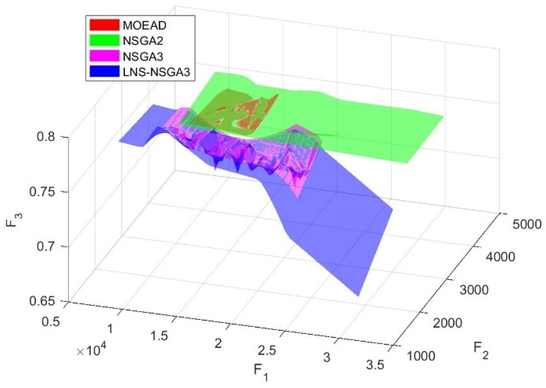
Furthermore, as shown in Figure 10, we compare the solution set surfaces of the four algorithms on a three-dimensional plane (each dimension representing an optimization objective). It can be seen that in three-dimensional space, the solution set surfaces of the MOEAD algorithm and the NSGA2 algorithm overlap significantly, indicating that there is not much difference between the two algorithms in terms of the freshness optimization objective. The NSGA3 and LNSNSGA3 algorithms, on the other hand, have a steeper position in the three-dimensional space, indicating that these two algorithms have stronger local search capabilities.

By comparing

Table 6. Performance comparison of different algorithms.

Algorithm	Optimal Solution with Lowest Cost	Optimal Solution with Lowest Carbon Emissions	Optimal Solution with Highest Freshness	Cput (s)
MOEAD	[11805.71, 2760.02, 0.7686]	[11805.71, 2760.02, 0.7686]	[13290.09, 3167.65, 0.7711]	150
NSGA2	[11128.22, 2630.08, 0.7707]	[11128.22, 2630.08, 0.7707]	[14117.81, 3386.83, 0.7716]	160
NSGA3	[10132.59, 2382.36, 0.7733]	[12853.35, 2213.56, 0.7650]	[10132.59, 2382.36, 0.7733]	180
LNSNSGA3	[7881.29, 1796.09, 0.8036]	[7944.99, 1712.22, 0.8101]	[8651.19, 1948.39, 0.8139]	210

, we extract the best solutions after 300 iterations for the four algorithms, specifically the optimal solutions for the lowest cost, the lowest carbon emissions, and the highest freshness. From the data in the table, it can be seen that for the optimal solution targeting the lowest cost, the LNSNSGA3 algorithm is superior to the NSGA3, NSGA2, and MOEAD algorithms by 28.5%, 41.19%, and 49.79%, respectively. For the optimal solution targeting the lowest carbon emissions, it is superior by 29.3%, 53.6%, and 61.19%, respectively. For the optimal solution targeting the highest average freshness, it is superior by 5.25%, 5.48%, and 5.55%, respectively. In terms of solving time (Cput), it is superior by −16.67%, −31.25%, and −40%, respectively. In solving the three objectives, the LNSNSGA3 algorithm outperforms the other algorithms; although the solving time is higher, it amply demonstrates the superiority of the LNSNSGA3 algorithm’s solving performance.

5.4. Analysis of Vehicle Routing Optimization Results

In this section, firstly, this paper compares the vehicle routing distribution schemes before and after optimization, as shown in Figure 11. Figure 11 (left) shows the optimal delivery routes obtained before the optimization. It can be seen that the vehicle delivery routes before optimization are quite disordered and difficult to observe, with many intersections between different vehicle delivery routes. In contrast, the vehicle routing distribution scheme after optimization, as shown in Figure 11 (right), clearly shows the delivery routes of different vehicles, with fewer intersections between the delivery routes of different vehicles.

Additionally, by comparing the optimization objectives before and after optimization, as shown in

Table 7. Comparison of various optimization objectives before and after path optimization.

	F1	F2	F3
Before optimization	9453.3	1964.6	0.7749
After optimization	7939.1	1710.5	0.7919

, it can be seen that all the optimization objectives after optimization have been improved to some extent compared to those before optimization, indicating that the optimization method used in this paper is better in solving this problem.

Taking the optimized delivery scheme as the control group, the following text will verify the experimental conclusions of this paper through different experiments. Since this paper considers the multi-vehicle type, multi-objective vehicle delivery path optimization problem under traffic congestion, the traffic congestion coefficient (TCC) is divided into the overall traffic congestion coefficient (OTCC) and regional traffic congestion coefficient (TCC-S) for research. Among them, TCC-S has a corresponding TCC for each region, which affects the average delivery speed of vehicles, thereby affecting the delivery cost, carbon emissions, and freshness of goods. As shown in

Table 8. Impact of OTCC on optimization objectives.

OTCC	F1		F2		F3
1	7748.21	+2.40%	1654.59	+3.27%	0.8191	+3.43%
1.1	7784.69	+1.94%	1665.27	+2.64%	0.816	+3.04%
1.2	7797.29	+1.79%	1668.96	+2.43%	0.8131	+2.68%
1.3	7898.96	+0.51%	1698.75	+0.69%	0.8101	+2.30%
1.4	8033.32	−1.19%	1738.11	−1.61%	0.8072	+1.93%
1.5	8188.06	−3.14%	1783.43	−4.26%	0.8044	+1.58%
1.6	8355.37	−5.24%	1832.45	−7.13%	0.8015	+1.21%
1.7	8530.28	−7.45%	1883.68	−10.12%	0.7985	+0.83%
1.8	8709.52	−9.70%	1936.19	−13.19%	0.7957	+0.48%
1.9	8890.97	−11.99%	1989.35	−16.30%	0.7926	+0.09%
2.0	9073.23	−14.29%	2042.74	−19.42%	0.7894	−0.32%
2.1	9255.39	−16.58%	2096.1	−22.54%	0.7864	−0.69%
2.2	9436.87	−18.87%	2149.26	−25.65%	0.7832	−1.10%
2.3	9617.29	−21.14%	2202.11	−28.74%	0.78	−1.50%
2.4	9796.43	−23.39%	2254.59	−31.81%	0.777	−1.88%
2.5	9974.17	−25.63%	2306.66	−34.85%	0.7739	−2.27%
2.6	10150.46	−27.85%	2358.3	−37.87%	0.7709	−2.65%
2.7	10325.29	−30.06%	2409.51	−40.87%	0.7678	−3.04%
2.8	10672.73	−34.43%	2460.31	−43.84%	0.7647	−3.43%
2.9	11038.44	−39.04%	2510.69	−46.78%	0.7617	−3.81%
3.0	11402.81	−43.63%	2560.68	−49.70%	0.7587	−4.19%

‘+’ indicates better compared to control, ‘−’ indicates worse compared to control.

, this paper considers the impact of OTCC on the optimization objectives, using the control group (TCC-S) vehicle delivery path scheme unchanged, adjusting OTCC from 1 to 3 with a step of 0.1, representing the transition from smooth traffic to traffic congestion.

By comparing the results in the table, it can be seen that when the OTCC is less than 1.4, the optimization objectives F1 and F2 of the experimental group are superior to the results of the control group. When the OTCC is less than 2.0, the optimization objective F3 of the experimental group is superior to the results of the control group. This indicates that compared to F3, F1 and F2 are more significantly influenced by OTCC. Meanwhile, F1 and F2 perform better within the range of 1.0 to 1.3, which might be because, in the case of low congestion, the overall traffic conditions across the network are relatively favorable, and the OTCC is more conducive to global route optimization, as it allows the utilization of a wider range of road resources. In contrast, the TCC-S might focus more on local optimization, potentially neglecting the possibility of achieving global optimization. However, within the service time window of the distribution center, the average value of TCC is obviously greater than 1.4, indicating that the TCC-S considered in this paper is more practical.

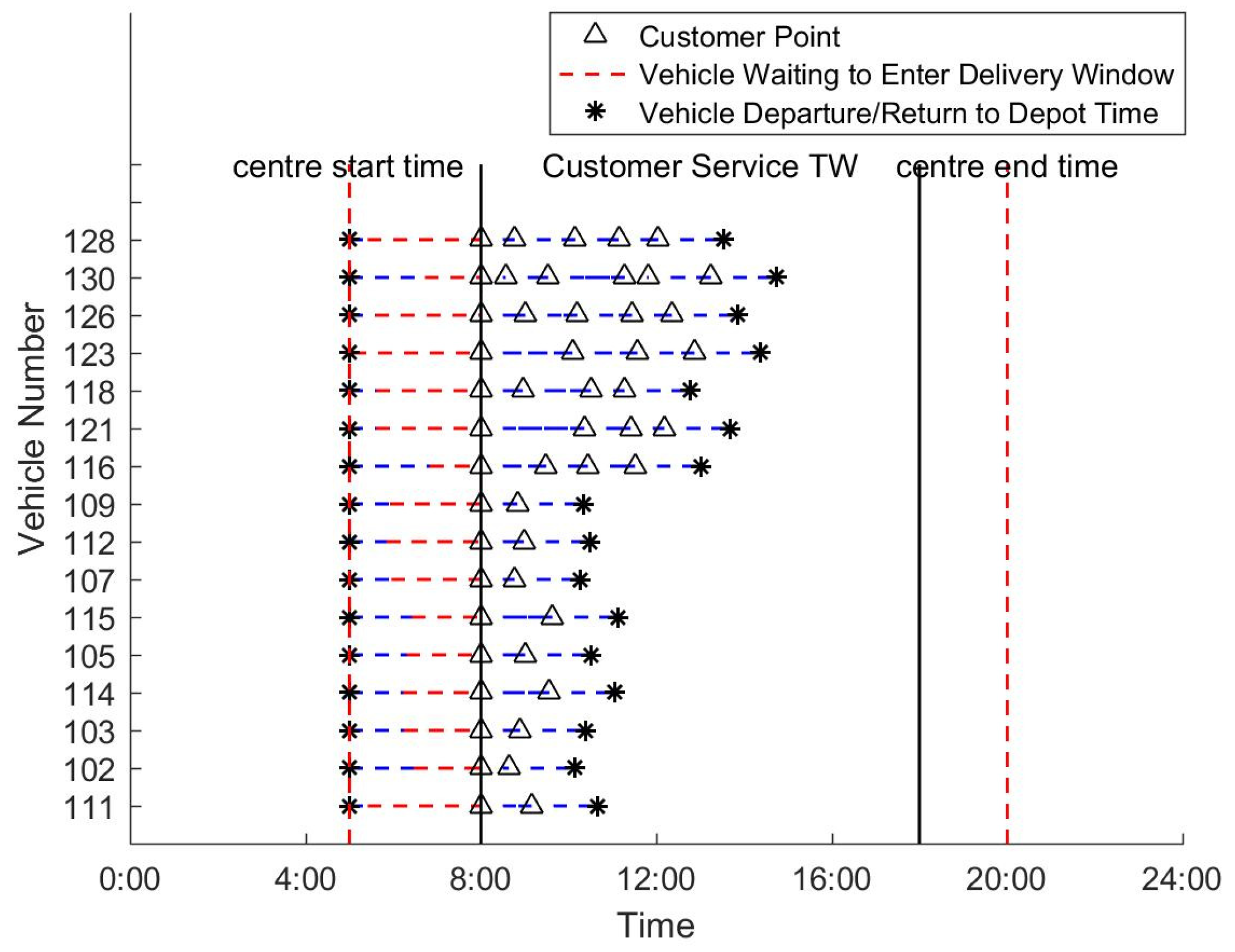
Meanwhile, according to the provisions in this paper, the time when the vehicle leaves the distribution center is the earliest service time of the distribution center, and it is required that the vehicle must serve within the customer service time window. Taking the control group as the benchmark, a time schedule diagram of the vehicle delivery path scheme is drawn.

From Figure 12, it can be seen that after leaving the distribution center, each vehicle needs to wait for a period of time to enter the initial service time window of the customer before starting to execute the delivery task. This will lead to a decrease in the freshness of goods when delivered to customers because the freshness of goods will decrease with the length of time after leaving the distribution center and the influence of refrigeration temperature. Therefore, under the condition of a constant refrigeration temperature, a longer waiting time is not conducive to optimizing objective F3. Therefore, in order to effectively improve the result of optimization objective F3, it is assumed that the waiting time for vehicles to enter the customer service time window will be minimized, and the vehicle departure time will be dynamically adjusted. The adjusted vehicle delivery time scheme is shown in Figure 13.

As shown in Figure 13, after adjusting the departure time of the vehicles, each vehicle has a certain delay in leaving the distribution center, ensuring the earliest service window for customers. Meanwhile, as shown in

Table 9. Comparison of optimization objectives before and after adjustment.

	F1	F2	F3
Before adjustment	7939.1	1710.5	0.7919
After adjustment	7948.99	1713.40	0.8315

, the optimization results for objectives F1 and F2 slightly increased. This might be due to the fact that after the vehicles’ departure time was delayed, their departure times fell within the ‘morning rush hour,’ during which the average congestion index increased. In contrast to optimization objective F3, the optimized result improved by 5% compared to before, effectively enhancing the average freshness of goods delivered to customers, which aligned with the goal of adjusting the departure time, as mentioned earlier.

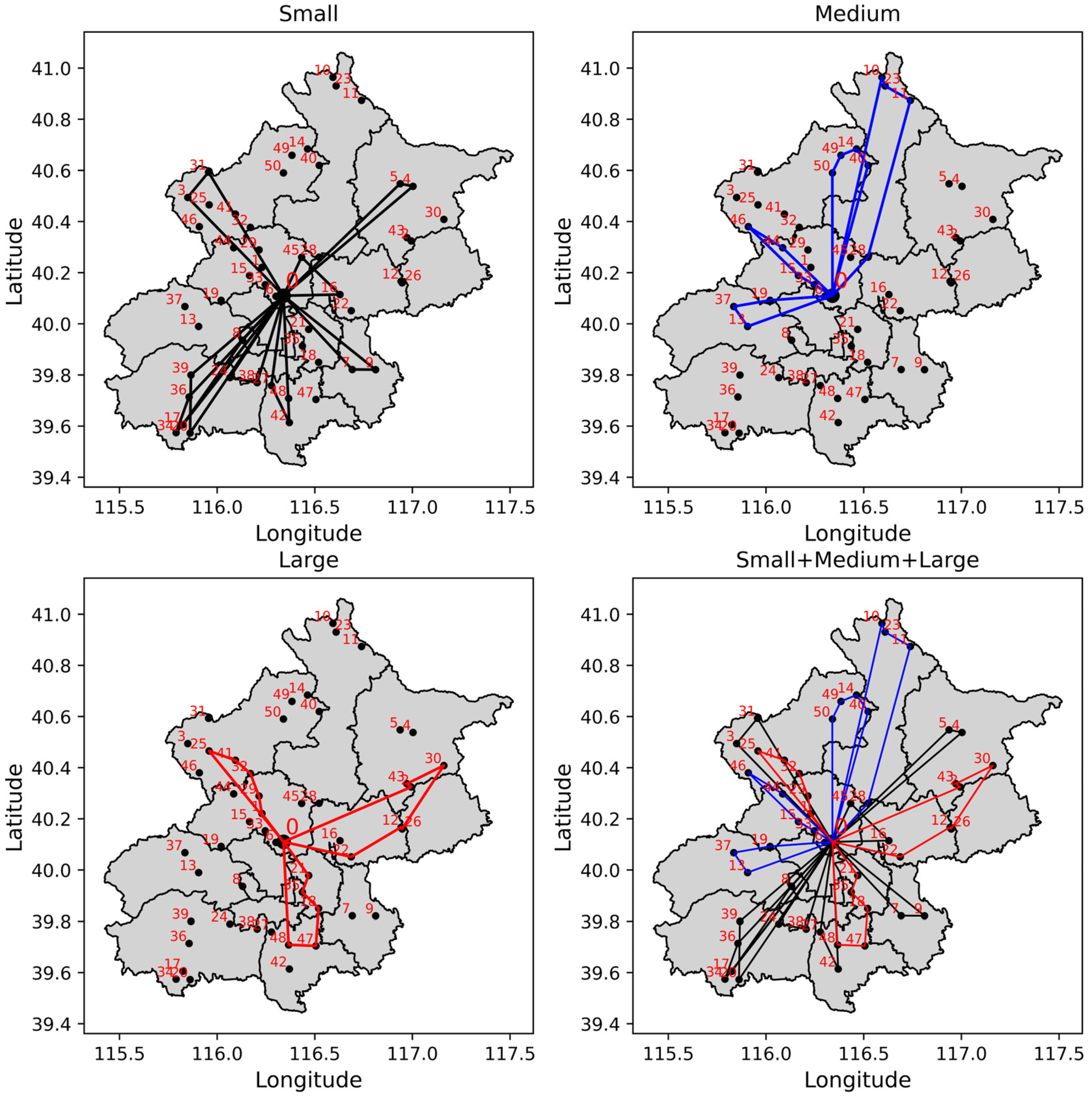
Secondly, using the control group as a reference, we analyze the impact of multi-vehicle models on vehicle distribution. First, as shown in

Table 10. Comparison of delivery results for different vehicle models.

K	Distribution Programme	Vnum	f1	f2	f3	f4	F1	F2	F3
Small	0-45-16-0	9	100	116.56	5.46	0.00	222.02	35.75	0.8469
	0-5-4-0		100	342.44	16.05	0.00	458.48	105.01	0.8531
	0-31-3-0		100	221.51	10.38	0.00	331.89	67.93	0.8499
	0-39-20-0		100	319.80	14.99	0.00	434.78	98.07	0.8422
	0-36-34-0		100	282.76	13.25	0.00	396.01	86.71	0.8486
	0-17-8-0		100	264.87	12.41	0.00	377.28	81.23	0.8414
	0-24-38-0		100	172.65	8.09	0.00	280.74	52.95	0.8515
	0-27-42-0		100	188.75	8.84	0.00	297.60	57.88	0.8490
	0-7-9-0		100	184.47	8.64	0.00	293.12	56.57	0.8507
Medium	0-50-49-14-40-0	4	150	523.51	24.53	0.00	698.04	160.54	0.8173
	0-28-11-23-10-0		150	549.56	25.75	0.00	725.31	168.53	0.8033
	0-44-46-15-33-0		150	242.07	11.34	0.00	403.42	74.24	0.8214
	0-6-19-37-13-0		150	415.34	19.46	0.00	584.80	127.37	0.8003
Large	0-21-35-18-47-48-0	3	200	522.56	24.49	0.00	747.05	160.25	0.8098
	0-2-43-30-26-12-22-0		200	752.72	35.27	0.00	987.99	230.83	0.8054
	0-1-29-32-41-25-0		200	487.61	22.85	0.00	710.46	149.53	0.8138
Total		16	2100	5587.18	261.81	0.00	7948.99	1713.40	0.8315

below, it can be seen that the fixed cost (f1), fuel cost (f2), carbon emission cost (f3), and time penalty cost (f4) of this distribution plan are 2100, 5587.18, 261.81, and 0 yuan respectively, with a total cost (F1) of 7948.99 yuan. The total carbon emissions (F2) are 1713.40 kg, the average freshness for customers delivered by Small vehicles is approximately 0.8400, by Medium vehicles is approximately 0.8100, by Large vehicles is approximately 0.8000, and the total average freshness (F3) is 0.8315.

Drawing four delivery route maps for Small, Medium, Large, and Small + Medium + Large vehicles, as shown in Figure 14, we can see that this distribution plan uses Small, Medium, and Large vehicles, with nine Small vehicles, four Medium vehicles, and three Large vehicles used.

As shown in Figure 14, considering the delivery strategy of Small + Medium + Large vehicles, to understand the impact of vehicle models on the optimization results, this article also adopted several delivery strategies such as All-Small, All-Medium, All-Large, Small+Medium, Small+Large, and Medium+Large, and solved the optimization results of these strategies. A comparison of Vnum, f1, f2, f3, f4, F1, F2, and F3 is shown in

Table 11. Comparison of delivery results for different vehicle model combinations.

Combinatorial	Vnum	f1	f2	f3	f4	F1	F2	F3
All-Small	25	2500	6052.1	283.6	0	8835.7	1856	0.8387
All-Medium	13	1950	7043.5	330	0	9323.5	2160	0.7490
All-Large	7	1400	10481	491.1	10,588	22,960	3214.1	0.6235
Small + Medium	20	2300	6780	317.7	0	9397.5	2079.2	0.7918
Small + Large	16	1900	8469.2	396.9	4859.7	15,626	2597.2	0.7859
Medium + Large	11	1800	9009	422.1	2240	13,471	2762.8	0.6843
Small + Medium + Large	16	2100	5587.18	261.81	0	7948.99	1713.4	0.8315

.

From Table 11, it can be seen that in terms of the number of vehicles used, the All-Large strategy uses the fewest vehicles. In terms of f4 (time penalty cost), only the All-Small, All-Medium, Small+Medium, and Small+Medium+Large strategies did not incur time penalty costs. In the comparison of Vnum, F1, F2, and F3, using the Small+Medium+Large strategy as the control group, the experimental results differences with other strategies are compared, as shown in

Table 12. Differences in delivery results for different vehicle model combinations.

Combinatorial	Vnum	F1	F2	F3
All-Small	−56.25%	−11.16%	−8.32%	+0.87%
All-Medium	+18.75%	−17.29%	−26.07%	−9.92%
All-Large	+56.25%	−188.84%	−87.59%	−25.02%
Small+Medium	−25.00%	−18.22%	−21.35%	−4.77%
Small+Large	0%	−96.58%	−51.58%	−5.48%
Medium+Large	+31.25%	−69.47%	−61.25%	−17.70%

‘+’ indicates better compared to control, ‘−’ indicates worse compared to control.

.

From Table 12, it can be seen that compared to the control group, except for the All-Small and Small+Medium strategies, the Vnum values of the other strategies are all better than that of the control group. In terms of F1 and F2, the results of the control group are superior to those of the other strategies. Regarding F3, only the result of the All-Small strategy is better than that of the control group. This is because, although the All-Small strategy uses more vehicles, the delivery speed is higher than that of the control group; therefore, the result of the optimization objective F3 is better than that of the control group.

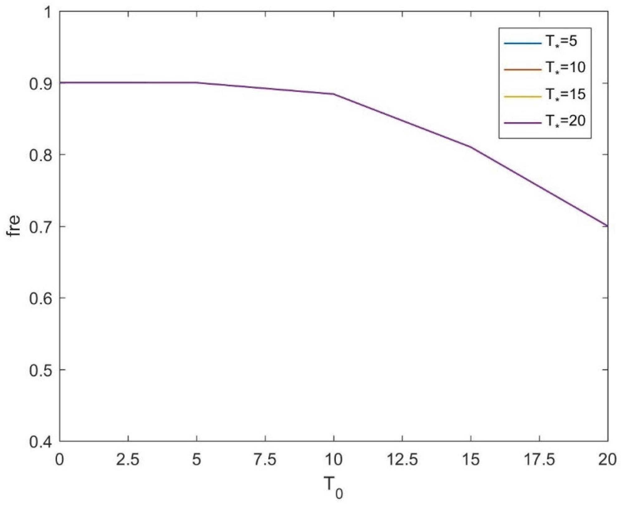
Finally, based on Equations (25) and (26), disregarding the intrinsic properties of goods, we investigated the relationship between the optimization target F3 (average freshness) and the duration of goods leaving the distribution center, environmental temperature, and refrigeration temperature during vehicle transport. Firstly, using the control group from the previous text as a benchmark, we fixed the duration of goods leaving the distribution center and conducted comparative experiments considering different environmental temperatures ($T_{*}=5 °\mathrm{C},10 °\mathrm{C},15 °\mathrm{C},20 °\mathrm{C}$) and different refrigeration temperatures inside the carriage ($T_0=0 °\mathrm{C},5 °\mathrm{C},10 °\mathrm{C}.15 °\mathrm{C},20 °\mathrm{C}$). The experimental results are shown in Figure 15.

From Figure 15, it can be observed that under different external environmental temperature conditions, the relationship curves between the optimization target F3 and the refrigeration temperature inside the carriage fully overlap, indicating identical experimental results. This suggests that the external environmental temperature during transportation does not affect the freshness of goods, with the refrigeration temperature inside the carriage being the most influential factor. Additionally, the figure shows that as the refrigeration temperature inside the carriage increases, the average freshness of the goods decreases when they reach the customer. This indicates that to optimize F3 and increase freshness, businesses need to maintain a higher refrigeration temperature during transport. Secondly, we studied the relationship between refrigeration temperature and cost and carbon emissions under different external environmental temperatures, with the experimental results shown in Figure 16.

From Figure 16, it is evident that under the same refrigeration temperature, as the environmental temperature increases, the distribution cost and carbon emissions also increase. Under the same external environmental temperature, when the refrigeration temperature is higher than the environmental temperature, increasing the carriage refrigeration temperature leads to an increased distribution cost and carbon emissions. Conversely, when the refrigeration temperature is lower than the environmental temperature, increasing the carriage refrigeration temperature reduces the distribution cost and carbon emissions until the refrigeration temperature equals the environmental temperature, where the cost and carbon emissions are at their minimum. This is because when the environmental temperature matches the vehicle refrigeration temperature, the refrigeration engine inside the carriage defaults to stop working, ceasing the fuel consumption associated with it. This indicates that cold chain logistics transportation during high external environmental temperatures results in higher costs and carbon emissions; additionally, the lower the carriage refrigeration temperature, the higher the transportation cost and carbon emissions.

6. Conclusions and Future Outlook

In this study, symmetry served as a key theoretical framework that has permeated multiple research stages, particularly in the solution design for multi-objective optimization and cross-regional distribution problems. The main conclusions regarding the application of the symmetry concept in this research are as follows:

(1)

The LNSNSGA-III algorithm balances the symmetry points among the cost, carbon emissions, and average freshness, thereby efficiently allocating resources across conflicting objectives.

(2)

Regional traffic congestion coefficients ensure a rational distribution of traffic conditions across regions, dynamically adjust vehicle speed, fuel consumption, and delivery times based on regional traffic, and enhance system stability.

(3)

In multi-vehicle distribution strategies, symmetry is achieved through the reasonable matching of vehicle types with delivery routes, improving efficiency, and reducing resource waste.

(4)

Optimizing departure times balances the temporal symmetry in the delivery process, significantly improving average freshness while avoiding peak-hour deliveries and reducing traffic congestion impacts.

(5)

In cold chain logistics, maintaining an appropriate refrigeration temperature has a direct symmetric relationship with average freshness, emphasizing the importance of consistent refrigeration conditions during transportation.

In summary, the symmetry concept permeated various aspects of this research, including multi-objective optimization, traffic congestion coefficients across regions, vehicle combination and route optimization, departure time management, and refrigeration temperature control. By introducing symmetric designs in different research stages, this study not only enhanced the overall efficiency of the delivery system but also achieved balance and coordination among optimization objectives. In the future, as traffic conditions and real-time data become increasingly complex, distribution strategies based on the symmetry concept will become more flexible and efficient, thereby providing competitive solutions for the sustainable development of the logistics industry.