Equivalence of History and Generator ϵ-Machines

Abstract

$ϵ$-Machines are minimal, unifilar presentations of stationary stochastic processes. They were originally defined in the history machine sense as hidden Markov models whose states are the equivalence classes of infinite pasts with the same probability distribution over futures. In analyzing synchronization though, an alternative generator definition was given as follows: unifilar, edge-emitting hidden Markov models with probabilistically distinct states. The key difference is that history $ϵ$-machines are defined by a process, whereas generator $ϵ$-machines define a process. We show here that these two definitions are equivalent in the finite-state case.

1. Introduction

Let $\mathcal{P}={(X_t)}_{t\in \mathbb{Z}}$ be a stationary stochastic process. The $ϵ$-machine $M=M(\mathcal{P})$ for the process $\mathcal{P}$ is the hidden Markov model whose states consist of equivalence classes of infinite past sequences (histories) $\overleftarrow{x}=\dots x_{-2}{x}_{-1}$ with the same probability distribution over future sequences $\overrightarrow{x}=x_0{x}_1\dots$. The corresponding equivalence relation on the set of pasts $\overleftarrow{x}$ is denoted by ${\sim }_{ϵ}$ as follows:

$$\begin{array}{c}\hfill \overleftarrow{x}{\sim }_{ϵ}{\overleftarrow{x}}^{\prime }\mathrm{if}\mathbb{P}(\overrightarrow{X}|\overleftarrow{x})=\mathbb{P}(\overrightarrow{X}|{\overleftarrow{x}}^{\prime }),\end{array}$$

(1)

where $\overrightarrow{X}=X_0{X}_1\dots$ denotes the infinite sequence of future random variables.

These machines were first introduced in [1] as minimal, predictive models to measure the structural complexity of dynamical systems and have subsequently been applied in a number of contexts for nonlinear modeling [2,3,4,5,6]. Important extensions and a more thorough development of the theory were given in [7,8,9,10]. However, it was not until quite recently that the first fully formal construction was presented in [11,12,13].

Shortly thereafter, in our studies of synchronization [14,15], we introduced an alternative “generator $ϵ$-machine” definition, in contrast to the original “history $ϵ$-machine” construction discussed above. A generator $ϵ$-machine is defined simply as a unifilar, edge-emitting hidden Markov model with probabilistically distinct states. As opposed to the history $ϵ$-machine $M_h=M_h(\mathcal{P})$ which is derived from a process $\mathcal{P}$, a generator $ϵ$-machine $M_g$ itself defines a stationary process $\mathcal{P}=\mathcal{P}(M_g)$. Namely, the stationary output process of the hidden Markov model $M_g$ is obtained by choosing the initial state according to the stationary distribution $\pi$ for states of the underlying Markov chain.

The main contribution established here is that the history and generator $ϵ$-machine definitions are equivalent in the finite state case. This has long been assumed, without formally specifying the generator definition. However, our work makes this explicit and gives one of the first formal proofs of equivalence.

The equivalence is also implicit in [16]; in fact, this is the case for a more general class of machines, not just finite-state ones. However, the techniques used there differ substantially from ours and use somewhat more machinery. In particular, the proof of equivalence in the more difficult direction of Theorem 1 (Section 4.1) uses a supermartingale argument that, though elegant, relies implicitly on the martingale convergence theorem and is not particularly concrete. By contrast, our proof of Theorem 1 follows directly from the synchronization results given in [14,15], which are themselves fairly elementary, using only basic information theory and a large deviation estimate for finite-state Markov chains. Thus, the alternative proof presented here should be useful in providing intuition for the theorem. Furthermore, since the definitions and terminology used in [16] differ significantly from ours, it is not immediately clear that the history-generator equivalence is what is shown there or whether this is a consequence of what is shown. Thus, the exposition here should be helpful in clarifying these issues.

We note also that in order to parallel the generator $ϵ$-machine definition used in our synchronization studies and apply the results from those works, we somewhat restrict the range of processes when defining history $ϵ$-machines. In particular, we assume when defining history $ϵ$-machines that the process $\mathcal{P}$ is not only stationary but also ergodic and that the process alphabet is finite. This is required for equivalence, since the output process of a generator $ϵ$-machine is of this form. However, neither of these assumptions is strictly necessary for history $ϵ$-machines. Only stationarity is actually needed. The history $ϵ$-machine definition can be extended to nonergodic stationary processes and countable or even more general alphabets [9,16].

2. Related Work

Since their introduction in the late 1980s, most of the work on $ϵ$-machines, both theoretical and applied, has come from physics and information theory perspectives. However, similar concepts have been around for some time in several other disciplines. Among others, there has been substantial work on related topics by both probabilists and automata theorists, as well as those in the symbolic dynamics community. Below, we review some of the most germane developments in these areas. The interested reader is also referred to ref. [9] (appendix H) where a very broad overview of such connections is given and to ref. [17] for a recent review of the relation between symbolic dynamics and hidden Markov models in general.

We hope that our review provides context for the study of $ϵ$-machines and helps elucidate the relationship between $ϵ$-machines and other related models—both in terms of their similarities and their differences. However, an understanding of these relationships will not be necessary for the equivalence results that follow. The reader uninterested in these connections may safely skip to the definitions in Section 3.

2.1. Sofic Shifts and Topological Presentations

Let $\mathcal{X}$ be a finite alphabet, and let ${\mathcal{X}}^{\mathbb{Z}}$ denote the set of all bi-infinite sequences $\overleftrightarrow{x}=\dots x_{-1}{x}_0{x}_1\dots$ consisting of symbols in $\mathcal{X}$. A subshift $\Sigma \subset {\mathcal{X}}^{\mathbb{Z}}$ is said to be sofic if it is the image of a subshift of a finite type under a k-block factor map. This concept was first introduced in [18], where it was also shown that any sofic shift $\Sigma$ may be presented as a finite, directed graph with edges labeled by symbols in the alphabet $\mathcal{X}$. The allowed sequences $\overleftrightarrow{x}\in \Sigma$ consist of projections (under the edge labeling) of bi-infinite walks on the graph edges.

In the following, we will assume that all vertices in a presenting graph G of a sofic shift are essential. That is, each vertex v occurs as the target vertex of some edge e in a bi-infinite walk on the graph edges. If this is not the case, one may be restricted to the graph $G^{\prime }$, which consists of essential vertices in G, along with their outgoing edges, and $G^{\prime }$ will also be a presenting graph for the sofic shift $\Sigma$. Thus, it is only necessary to consider presenting graphs in which all vertices are essential.

The language $Ł(\Sigma )$ of a subshift $\Sigma$ is the set of all finite words w occurring in some point $\overleftrightarrow{x}\in \Sigma$. For a sofic shift $\Sigma$ with a presenting graph G, one may consider the nondeterministic finite automaton (NFA) M associated with the graph G, in which all states (vertices of G) are both start and accept states. Clearly (under the assumption that all vertices are essential), the language accepted by M is just $Ł(\Sigma )$. Thus, the language of any sofic shift is regular. By standard algorithms (see e.g., [19]) one may obtain from M a unique, minimal, deterministic finite automaton (DFA) $M^{\prime }$ with the fewest number of states of all DFAs accepting the language $Ł(\Sigma )$. We call $M^{\prime }$ the minimal deterministic automaton for the sofic shift $\Sigma$.

A subshift $\Sigma$ is said to be irreducible if for any two words $w_1,w_2\in Ł(\Sigma )$ there exists $w_3\in Ł(\Sigma )$ such that the word is $w_1{w}_3{w}_2\in Ł(\Sigma )$. As shown in [20], a sofic shift is irreducible if and only if it has some irreducible (i.e., strongly connected) presenting graph G.

A presenting graph G of a sofic shift $\Sigma$ is said to be unifilar or right-resolving if for each vertex $v\in G$ and symbol $x\in \mathcal{X}$ there is at most one outgoing edge e from v labeled with the symbol x. A shown in [21], an irreducible sofic shift $\Sigma$ always has a unique, minimal, unifilar presenting graph that, as it turns out, is also irreducible. In symbolic dynamics, this presentation is often referred to as the (right) Fischer cover of $\Sigma$.

For an irreducible sofic shift $\Sigma$, the graph associated with the minimal deterministic automaton always has a single recurrent, irreducible component. This recurrent component is isomorphic to the Fischer cover. That is, there exists a bijection between vertices in the automaton graph and vertices of the Fischer cover that preserves both edges and edge labels.

A related notion is the Krieger cover based on future sets [22]. For a subshift $\Sigma \subset {\mathcal{X}}^{\mathbb{Z}}$, let ${\Sigma }^{+}$ denote the set of allowed future sequences $\overrightarrow{x}=x_0{x}_1\dots$ and let ${\Sigma }^{-}$ be the set of allowed past sequences $\overleftarrow{x}=\dots x_{-2}{x}_{-1}$. This is expressed as follows:

$$\begin{array}{c}\hfill {\Sigma }^{+}=\{\overrightarrow{x}:\exists \overleftarrow{x} \mathrm{with} \overleftarrow{x}\overrightarrow{x}\in \Sigma \} \mathrm{and} {\Sigma }^{-}=\{\overleftarrow{x}:\exists \overrightarrow{x} \mathrm{with} \overleftarrow{x}\overrightarrow{x}\in \Sigma \}.\end{array}$$

Furthermore, for a past $\overleftarrow{x}\in {\Sigma }^{-}$, let the future set $F(\overleftarrow{x})$ of $\overleftarrow{x}$ be the set of all possible future sequences $\overrightarrow{x}$ that can follow $\overleftarrow{x}$:

$$\begin{array}{c}\hfill F(\overleftarrow{x})=\{\overrightarrow{x}\in {\Sigma }^{+}:\overleftarrow{x}\overrightarrow{x}\in \Sigma \}.\end{array}$$

Define an equivalence relation ${\sim }_K$ on the set of infinite pasts $\overleftarrow{x}\in {\Sigma }^{-}$ by the following:

$$\begin{array}{c}\hfill \overleftarrow{x}{\sim }_K{\overleftarrow{x}}^{\prime } \mathrm{if} F(\overleftarrow{x})=F({\overleftarrow{x}}^{\prime }).\end{array}$$

(2)

The Krieger cover of $\Sigma$ is the (possibly infinite) directed, edge-labeled graph G, whose vertices consist of equivalence classes of pasts $\overleftarrow{x}$ under the relation ${\sim }_K$. There is a directed edge in G from vertex v to vertex $v^{\prime }$ labeled with symbol x, if for some past $\overleftarrow{x}\in v$ (equivalently all pasts $\overleftarrow{x}\in v$) the past ${\overleftarrow{x}}^{\prime }=\overleftarrow{x}x\in v^{\prime }$. By construction, the Krieger cover G is necessarily unifilar. Moreover, it is easily shown that G is a finite graph if and only if the subshift $\Sigma$ is sofic.

If the subshift $\Sigma$ is both irreducible and sofic, then the Krieger cover is isomorphic to the subgraph of the minimal deterministic automaton consisting of all states v that are not $finite\text{-}time transient$ (and their outgoing edges). That is, the subgraph consisting of those states v such that there exist arbitrarily long words $w\in Ł(\Sigma )$ on which the automaton transitions from its start state to v. Clearly, any state in the recurrent, irreducible component of the automaton graph is not finite-time transient. Thus, the Krieger cover contains this recurrent component—the Fischer cover.

To summarize, the minimal deterministic automaton, Fischer cover, and Krieger cover are three closely related ways for presenting an irreducible sofic shift that are each, in slightly different senses, minimal unifilar presentations. The Fischer cover is always an irreducible graph. The Krieger cover and graph of the minimal deterministic automaton are not necessarily irreducible, but they each have a single recurrent, irreducible component that is isomorphic to the Fischer cover. The Krieger cover itself is also isomorphic to a subgraph of the minimal deterministic automaton.

$ϵ$-Machines are a probabilistic extension of these purely topological presentations. More specifically, for a stationary process $\mathcal{P}$, the history $ϵ$-machine $M_h$ is the probabilistic analog of the Krieger cover G for the subshift consisting of $\mathrm{supp}(\mathcal{P})$. It is the edge-emitting hidden Markov model defined analogously to the Krieger cover, but with states that are equivalence classes of infinite past sequences $\overleftarrow{x}$ with the same probability distribution over future sequences $\overrightarrow{x}$, rather than simply the same set of allowed future sequences (Compare Equations (1) and (2)).

In some cases, the two presentations may be topologically equivalent, e.g., the history $ϵ$-machine and Krieger cover can be isomorphic as graphs when the transition probabilities are removed from edges of the $ϵ$-machine. In other cases, however, they are not. For example, for the Even Process (Example 1, Section 3.5) the Krieger cover (or at least its recurrent component, the Fischer cover) and the history $ϵ$-machine are topologically equivalent. However, this is not so for the ABC process (Example 2, Section 3.5). In fact, there exist many examples of ergodic processes whose support is an irreducible sofic shift, but for which the history $ϵ$-machine has an infinite (or even continuum) number of states. See, e.g., Example 4 in Section 3.5, and Example 3.26 in [16].

2.2. Semigroup Measures

Semigroup measures are a class of probability measures on sofic shifts that arise from assigning probability transition structures to the right and left covers obtained from the Cayley graphs associated with generating semigroups for the shifts. These measures are studied extensively in [23], where a rich theory is developed and many of their key structural properties are characterized.

In particular, it is shown there that a stationary probability measure $\mathbb{P}$ on a sofic shift $\Sigma$ is a semigroup measure if and only if it has a finite number of future measures—distributions over future sequences $\overrightarrow{x}$—induced by all finite-length past words w. That is, $\mathbb{P}$ is a semigroup measure if there exists a finite number of finite length words $w_1,\dots ,w_N$ such that for any word w the following positive probability holds:

$$\begin{array}{c}\hfill \mathbb{P}(\overrightarrow{X}|w)=\mathbb{P}(\overrightarrow{X}|w_i),\end{array}$$

for some $1\le i\le N$, where $\overrightarrow{X}$ denotes the infinite sequence of future random variables $X_t$ on $\Sigma$, defined by the natural projections $X_t(\overleftrightarrow{x})=x_t$.

By contrast, a process $\mathcal{P}$ (or measure $\mathbb{P}$) has a finite-state history $ϵ$-machine if there exists a finite number of infinite past sequences ${\overleftarrow{x}}_1,\dots ,{\overleftarrow{x}}_N$ such that, for almost every infinite past $\overleftarrow{x}$, the following stands:

$$\begin{array}{c}\hfill \mathbb{P}(\overrightarrow{X}|\overleftarrow{x})=\mathbb{P}(\overrightarrow{X}|{\overleftarrow{x}}_i),\end{array}$$

for some $1\le i\le N$. The latter condition is strictly more general. The Alternating Biased Coins Process described in Section 3.5, for instance, has a finite-state (2-state) $ϵ$-machine, but does not correspond to a semigroup measure.

Thus, unfortunately, though the theory of semigroup measures is quite rich and well developed, much of it does not apply for the measures we study. For this reason, our proof methods are quite different from those previously used for semigroup measures, despite the seeming similarity between the two settings.

2.3. g-Functions and g-Measures

For a finite alphabet $\mathcal{X}$, let ${\mathcal{X}}^{-}$ denote the set of all infinite past sequences $\overleftarrow{x}=\dots x_{-2}{x}_{-1}$ consisting of symbols in $\mathcal{X}$. A g-function for the full shift ${\mathcal{X}}^{\mathbb{Z}}$ is a map as follows:

$$\begin{array}{c}\hfill g:({\mathcal{X}}^{-}\times \mathcal{X})\to [0,1],\end{array}$$

such that for any $\overleftarrow{x}\in {\mathcal{X}}^{-}$, the following stands:

$$\begin{array}{c}\hfill \sum _{x\in \mathcal{X}}g(\overleftarrow{x},x)=1.\end{array}$$

A g-measure for a g-function g on the full shift ${\mathcal{X}}^{\mathbb{Z}}$ is stationary probability measure $\mathbb{P}$ on ${\mathcal{X}}^{\mathbb{Z}}$ that is consistent with the g-function g in that for $\mathbb{P}$ a.e. $\overleftarrow{x}\in {\mathcal{X}}^{-}$ as follows:

$$\begin{array}{c}\hfill \mathbb{P}(X_0=x|\overleftarrow{X}=\overleftarrow{x})=g(\overleftarrow{x},x), \mathrm{for} \mathrm{each} x\in \mathcal{X}.\end{array}$$

g-Functions and g-Measures have been studied for some time, though sometimes under different names [24,25,26,27]. In particular, many of these studies address cases where a g-function has or does not have a unique corresponding g-measure. Normally, g is assumed to be continuous (with respect to the natural product topology) and in this case, using fixed point theory, it can be shown that at least one g-measure exists. However, continuity is not enough to ensure uniqueness, even if some natural mixing conditions are required as well [26]. Thus, stronger conditions are often required, such as Hölder continuity.

Of particular relevance to us is the more recent work [28] on g-functions restricted to subshifts. This study shows, in many instances, ways of constructing g-functions on subshifts with an infinite or even continuum number of future measures, subject to fairly strong requirements; for example, residual local constancy or a synchronization condition similar to the exactness condition introduced in [15]. Most surprising, perhaps, are the constructions of g-functions for irreducible subshifts, which themselves take only a finite number of values, but have unique associated g-measures with an infinite number of future measures.

The relation to $ϵ$-machines is the following. Given a g-function g, one may divide the set of infinite past sequences $\overleftarrow{x}$ into equivalence classes, in a manner analogous to that for history $ϵ$-machines, by the relation ${\sim }_g$ as follows:

$$\begin{array}{c}\hfill \overleftarrow{x}{\sim }_g{\overleftarrow{x}}^{\prime } \mathrm{if} g(\overleftarrow{x},x)=g({\overleftarrow{x}}^{\prime },x), \mathrm{for} \mathrm{all} x\in \mathcal{X}.\end{array}$$

(3)

The equivalence classes induced by the relation ${\sim }_g$ of Equation (3) are coarser than those induced by the relation ${\sim }_{ϵ}$ of Equation (1). For any g-measure $\mathbb{P}$ of the g-function g, the states of the history $ϵ$-machine are a refinement or splitting of the ${\sim }_g$ equivalence classes. Two infinite pasts, $\overleftarrow{x}$ and ${\overleftarrow{x}}^{\prime }$, that induce different probability distributions over the next symbol $x_0$ must induce different probability distributions over infinite future sequences $\overrightarrow{x}$, but the converse is not necessarily true. As shown in [28], the splitting may in fact be quite “bad” even if “nice” conditions are enforced on the g-function associated with the probability measure $\mathbb{P}$. Concretely, there exist processes with history $ϵ$-machines that have an infinite or even continuum number of states, but for which the associated “nice” g-function from which the process is derived has only a finite number of equivalence classes.

3. Definitions

In this section, we set up the formal framework for our results and give more complete definitions for our objects of study as follows: stationary processes, hidden Markov models, and $ϵ$-machines.

3.1. Processes

There are several ways to define a stochastic process. Perhaps the most traditional definition is simply as a sequence of random variables $(X_t)$ on some common probability space $\Omega$. However, in the following discussion, it will be convenient to use a slightly different but equivalent construction in which a process is itself a probability space whose sample space consists of bi-infinite sequences $\overleftrightarrow{x}=\dots x_{-1}{x}_0{x}_1\dots$. Of course, on this space we have random variables $X_t$ defined by the natural projections $X_t(\overleftrightarrow{x})=x_t$, which we will at times employ in our proofs. However, for most of our development and, in particular, for defining history $ϵ$-machines, it will be more convenient to adopt the sequence-space viewpoint.

Throughout, we restrict our attention to processes over a finite alphabet $\mathcal{X}$. We denote by ${\mathcal{X}}^{\ast }$ the set of all words w of finite positive length consisting of symbols in $\mathcal{X}$ and, for a word $w\in {\mathcal{X}}^{\ast }$, we write $|w|$ for its length. Note that we deviate slightly from the standard convention here and explicitly exclude the null word $\lambda$ from ${\mathcal{X}}^{\ast }$.

Definition 1.

Let $\mathcal{X}$ be a finite set. A process $\mathcal{P}$ over the alphabet $\mathcal{X}$ is a probability space $({\mathcal{X}}^{\mathbb{Z}},\mathbb{X},\mathbb{P})$ where the following stand:

• ${\mathcal{X}}^{\mathbb{Z}}$ is the set of all bi-infinite sequences of symbols in $\mathcal{X}$: ${\mathcal{X}}^{\mathbb{Z}}=\{\overleftrightarrow{x}=\dots x_{-1}{x}_0{x}_1\dots :x_t\in \mathcal{X},\mathrm{for}\mathrm{all}t\in \mathbb{Z}\}$.
• $\mathbb{X}$ is the σ-algebra generated by finite cylinder sets of the form $A_{w,t}=\{\overleftrightarrow{x}\in {\mathcal{X}}^{\mathbb{Z}}:x_t\dots x_{t+|w|-1}=w\}$.
• $\mathbb{P}$ is a probability measure on the measurable space $({\mathcal{X}}^{\mathbb{Z}},\mathbb{X})$.

For each symbol $x\in \mathcal{X}$, we assume implicitly that $\mathbb{P}(A_{x,t})>0$ for some $t\in \mathbb{N}$. Otherwise, the symbol x is useless and the process can be restricted to the alphabet $\mathcal{X}/\left\{x\right\}$. In the following, we will be primarily interested in stationary, ergodic processes.

Let $r:{\mathcal{X}}^{\mathbb{Z}}\to {\mathcal{X}}^{\mathbb{Z}}$ be the right shift operator. A process $\mathcal{P}$ is stationary if the measure $\mathbb{P}$ is shift invariant as follows: $\mathbb{P}(A)=\mathbb{P}(r(A))$, for any measurable set A. A process $\mathcal{P}$ is ergodic if every shift invariant event A is trivial. That is, for any measurable event A such that A and $r(A)$ are $\mathbb{P}$ a.s. equal, the probability of A is either 0 or 1. A stationary process $\mathcal{P}$ is defined entirely by the word probabilities $\mathbb{P}(w)$, $w\in {\mathcal{X}}^{\ast }$, where $\mathbb{P}(w)=\mathbb{P}(A_{w,t})$ is the shift invariant probability of cylinder sets for the word w. Ergodicity is equivalent to the almost sure convergence of empirical word probabilities $\widehat{\mathbb{P}}(w)$ in finite sequences ${\overrightarrow{x}}^t=x_0{x}_1\dots x_{t-1}$ to their true values $\mathbb{P}(w)$, as $t\to \infty$.

For a stationary process $\mathcal{P}$ and words $w,v\in {\mathcal{X}}^{\ast }$ with $\mathbb{P}(v)>0$, we define $\mathbb{P}(w|v)$ as the probability where the word w is followed by the word v in a bi-infinite sequence $\overleftrightarrow{x}$ as follows:

$$\begin{array}{cc}\hfill \mathbb{P}(w|v)& \equiv \mathbb{P}(A_{w,0}|A_{v,-|v|})\hfill \\ \hfill & =\mathbb{P}(A_{v,-|v|}\cap A_{w,0})/\mathbb{P}(A_{v,-|v|})\hfill \\ \hfill & =\mathbb{P}(vw)/\mathbb{P}(v).\hfill \end{array}$$

(4)

The following facts concerning word probabilities and conditional word probabilities for a stationary process come directly from the definitions. They will be used repeatedly throughout our development, without further mention. For any words $u,v,w\in {\mathcal{X}}^{\ast }$, the following stand:

• ${\sum }_{x\in \mathcal{X}}\mathbb{P}(wx)={\sum }_{x\in \mathcal{X}}\mathbb{P}(xw)=\mathbb{P}(w)$.
• $\mathbb{P}(w)\ge \mathbb{P}(wv)$ and $\mathbb{P}(w)\ge \mathbb{P}(vw)$.
• If $\mathbb{P}(w)>0$, ${\sum }_{x\in \mathcal{X}}\mathbb{P}(x|w)=1$.
• If $\mathbb{P}(u)>0$, $\mathbb{P}(v|u)\ge \mathbb{P}(vw|u)$.
• If $\mathbb{P}(u)>0$ and $\mathbb{P}(uv)>0$, $\mathbb{P}(vw|u)=\mathbb{P}(v|u)·\mathbb{P}(w|uv)$.

3.2. Hidden Markov Models

There are two primary types of hidden Markov models as follows: state-emitting (or Moore) and edge-emitting (or Mealy). The state-emitting type is the simpler of the two and, also, the more commonly studied and applied [29,30]. However, we focus on edge-emitting hidden Markov models here, since $ϵ$-machines are edge-emitting. We also restrict our development to the case where the hidden Markov model has a finite number of states and output symbols, although generalizations to countably infinite and even uncountable state sets and output alphabets are certainly possible.

Definition 2.

An edge-emitting hidden Markov model (HMM) is a triple $(\mathcal{S},\mathcal{X},\left\{T^{(x)}\right\})$ model where the following stand:

• $\mathcal{S}$ is a finite set of states.
• $\mathcal{X}$ is a finite alphabet of output symbols.
• $T^{(x)},x\in \mathcal{X}$ are symbol-labeled transition matrices. $T_{\sigma {\sigma }^{\prime }}^{(x)}\ge 0$ represents the probability of transitioning from state σ to state ${\sigma }^{\prime }$ on symbol x.

In what follows, we normally take the state set to be $\mathcal{S}=\{{\sigma }_1,\dots ,{\sigma }_N\}$ and denote $T_{{\sigma }_i{\sigma }_j}^{(x)}$ simply as $T_{ij}^{(x)}$. We also denote the overall state-to-state transition matrix for an HMM as T: $T={\sum }_{x\in \mathcal{X}}{T}^{(x)}$. $T_{ij}$ is the overall probability of transitioning from state ${\sigma }_i$ to state ${\sigma }_j$, regardless of symbol. The matrix T is stochastic as follows: ${\sum }_{j=1}^N{T}_{ij}=1$, for each i.

Pictorially, an HMM can be represented as a directed graph with labeled edges. The vertices are the states ${\sigma }_1,\dots ,{\sigma }_N$ and, for each $i,j,x$ with $T_{ij}^{(x)}>0$, there is a directed edge from state ${\sigma }_i$ to state ${\sigma }_j$, labeled $p|x$ for the symbol x and transition probability $p=T_{ij}^{(x)}$. The transition probabilities are normalized so that their sum on all outgoing edges from each state ${\sigma }_i$ is 1.

Example. 

Even Machine

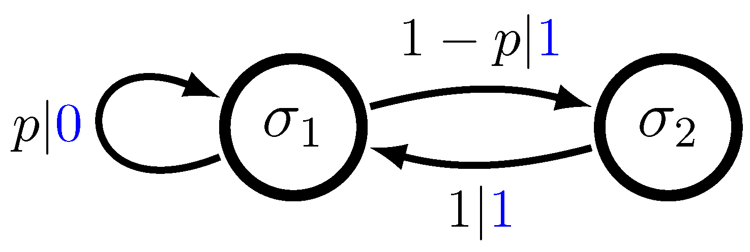
Figure 1 depicts an HMM for the Even Process. The support for this process consists of all binary sequences in which blocks of uninterrupted 1 s are even in length, bounded by 0 s. After each even length is reached, there is a probability p of breaking the block of 1 s by inserting a 0. The HMM has two states $\{{\sigma }_1,{\sigma }_2\}$ and symbol-labeled transitions matrices as follows:

$$\begin{array}{c}\hfill T^{(0)}=\left(\begin{array}{cc}p& 0\\ 0& 0\end{array}\right)\mathrm{and}{T}^{(1)}=\left(\begin{array}{cc}0& 1-p\\ 1& 0\end{array}\right)\end{array}$$

The operation of an HMM may be thought of as a weighted random walk on the associated directed graph. That is, from the current state ${\sigma }_i$, the next state ${\sigma }_j$ is determined by selecting an outgoing edge from ${\sigma }_i$ according to their relative probabilities. Having selected a transition, the HMM then moves to the new state and outputs the symbol x labeling this edge. The same procedure is then invoked repeatedly to generate future states and output symbols.

The state sequence determined in such a fashion is simply a Markov chain with transition matrix T. However, we are interested not simply in the HMM’s state sequence, but rather the associated sequence of output symbols it generates. We assume that an observer of the HMM has direct access to this sequence of output symbols, but not to the associated sequence of “hidden” states.

Formally, from an initial state ${\sigma }_i$, the probability that the HMM next outputs symbol x and transitions to state ${\sigma }_j$ is expressed as follows:

$$\begin{array}{c}\hfill {\mathbf{P}}_{{\sigma }_i}(x,{\sigma }_j)=T_{ij}^{(x)}.\end{array}$$

(5)

Furthermore, the probability of longer sequences is computed inductively. Thus, for an initial state ${\sigma }_i={\sigma }_{i_0}$, the probability the HMM outputs a length-l word $w=w_0\dots w_{l-1}$ while following the state path $s={\sigma }_{i_1}\dots {\sigma }_{i_l}$ in the next l steps is expressed as follows:

$$\begin{array}{c}\hfill {\mathbf{P}}_{{\sigma }_i}(w,s)=\prod _{t=0}^{l-1}{T}_{i_t,i_{t+1}}^{(w_t)}.\end{array}$$

(6)

If the initial state is chosen according to some distribution $\rho =({\rho }_1,\dots ,{\rho }_N)$ rather than as a fixed state ${\sigma }_i$, we obtain the following by linearity:

$$\begin{array}{cc}\hfill {\mathbf{P}}_{\rho }(x,{\sigma }_j)& =\sum _i{\rho }_i·{\mathbf{P}}_{{\sigma }_i}(x,{\sigma }_j) \mathrm{and}\hfill \end{array}$$

(7)

$$\begin{array}{cc}\hfill {\mathbf{P}}_{\rho }(w,s)& =\sum _i{\rho }_i·{\mathbf{P}}_{{\sigma }_i}(w,s).\hfill \end{array}$$

(8)

The overall probabilities of next generating a symbol x or word $w=w_0\dots w_{l-1}$ from a given state ${\sigma }_i$ are computed by summing over all possible associated target states or state sequences as follows:

$$\begin{array}{cc}\hfill {\mathbf{P}}_{{\sigma }_i}(x)& =\sum _j{\mathbf{P}}_{{\sigma }_i}(x,{\sigma }_j)={\parallel e_i{T}^{(x)}\parallel }_1 \mathrm{and}\hfill \end{array}$$

(9)

$$\begin{array}{cc}\hfill {\mathbf{P}}_{{\sigma }_i}(w)& =\sum _{\{s:|s|=l\}}{\mathbf{P}}_{{\sigma }_i}(w,s)={\parallel e_i{T}^{(w)}\parallel }_1,\hfill \end{array}$$

(10)

respectively, where $e_i=(0,\dots ,1,\dots ,0)$ is the $i^{\mathrm{th}}$ standard basis vector in ${\mathbb{R}}^N$ and

$$\begin{array}{cc}\hfill T^{(w)}& =T^{(w_0\dots w_{l-1})}\equiv \prod _{t=0}^{l-1}{T}^{(w_t)}.\hfill \end{array}$$

(11)

Finally, the overall probabilities of next generating a symbol x or word $w=w_0\dots w_{l-1}$ from an initial state distribution $\rho$ are, respectively, expressed as follows:

$$\begin{array}{cc}\hfill {\mathbf{P}}_{\rho }(x)& =\sum _i{\rho }_i·{\mathbf{P}}_{{\sigma }_i}(x)={\parallel \rho T^{(x)}\parallel }_1 \mathrm{and}\hfill \end{array}$$

(12)

$$\begin{array}{cc}\hfill {\mathbf{P}}_{\rho }(w)& =\sum _i{\rho }_i·{\mathbf{P}}_{{\sigma }_i}(w)={\parallel \rho T^{(w)}\parallel }_1.\hfill \end{array}$$

(13)

If the graph G associated with a given HMM is strongly connected, then the corresponding Markov chain over states is irreducible and the state-to-state transition matrix T has a unique stationary distribution $\pi$ satisfying $\pi =\pi T$ [31]. In this case, we may define a stationary process $\mathcal{P}=({\mathcal{X}}^{\mathbb{Z}},\mathbb{X},\mathbb{P})$ by the word probabilities obtained from choosing the initial state according to $\pi$. That is, for any word $w\in {\mathcal{X}}^{\ast }$ as follows:

$$\begin{array}{cc}\hfill \mathbb{P}(w)& \equiv {\mathbf{P}}_{\pi }(w)={\parallel \pi T^{(w)}\parallel }_1.\hfill \end{array}$$

(14)

Strong connectivity also implies the process $\mathcal{P}$ is ergodic, as it is a pointwise function of the irreducible Markov chain over edges, which is itself ergodic [31]. That is, at each time step, the symbol labeling the edge is a deterministic function of the edge.

We denote the corresponding (stationary, ergodic) process over bi-infinite symbol-state sequences $(\overleftrightarrow{x},\overleftrightarrow{s})$ by $\tilde{\mathcal{P}}$. That is, $\tilde{\mathcal{P}}=({(\mathcal{X} \mathrm{x} \mathcal{S})}^{\mathbb{Z}},(\mathbb{X} \mathrm{x} \mathbb{S}),\tilde{\mathbb{P}})$ where the following stand:

• ${(\mathcal{X} \mathrm{x} \mathcal{S})}^{\mathbb{Z}}=\left\{(\overleftrightarrow{x},\overleftrightarrow{s})\cong {(x_t,s_t)}_{t\in \mathbb{Z}}:x_t\in \mathcal{X} \mathrm{and} s_t\in \mathcal{S}, \mathrm{for} \mathrm{all} t\in \mathbb{Z}\right\}$.
• $(\mathbb{X} \mathrm{x} \mathbb{S})$ is the $\sigma$-algebra generated by finite cylinder sets on the bi-infinite symbol-state sequences.
• The (stationary) probability measure $\tilde{\mathbb{P}}$ on $(\mathbb{X} \mathrm{x} \mathbb{S})$ is defined by Equation (8) with $\rho =\pi$. Specifically, for any length-l word w and length-l state sequence s we have the following:

  $$\begin{array}{c}\hfill \tilde{\mathbb{P}}(\{(\overleftrightarrow{x},\overleftrightarrow{s}):x_0\dots x_{l-1}=w,s_1\dots s_l=s\})={\mathbf{P}}_{\pi }(w,s).\end{array}$$
  By stationarity, this measure may be extended uniquely to all finite cylinders and, hence, to all $(\mathbb{X} \mathrm{x} \mathbb{S})$-measurable sets. Furthermore, this is consistent with the measure $\mathbb{P}$ as follows:

  $$\begin{array}{c}\hfill \tilde{\mathbb{P}}(\{(\overleftrightarrow{x},\overleftrightarrow{s}):x_0\dots x_{l-1}=w\})=\mathbb{P}(w),\end{array}$$

  for all $w\in {\mathcal{X}}^{\ast }$.

Two HMMs are said to be isomorphic if there is a bijection between their state sets that preserves edges, including the symbols and probabilities labeling the edges. Clearly, any two isomorphic, irreducible HMMs generate the same process, but the converse is not true. Nonisomorphic HMMs may also generate equivalent processes. In Section 4, we will be concerned with isomorphism between generator and history $ϵ$-machines.

3.3. Generator $ϵ$-Machines

Generator $ϵ$-machines are irreducible HMMs with two additional important properties as follows: unifilarity and probabilistically distinct states.

Definition 3.

A generator ϵ-machine $M_g$ is an HMM with the following properties:

1.

Irreducibility: The graph G associated with the HMM is strongly connected.

2.

Unifilarity: For each state ${\sigma }_i\in \mathcal{S}$ and each symbol $x\in \mathcal{X}$, there is at most one outgoing edge from state ${\sigma }_i$ labeled with symbol x.

3.

Probabilistically distinct states: For each pair of distinct states ${\sigma }_i,{\sigma }_j\in \mathcal{S}$, there exists some word $w\in {\mathcal{X}}^{\ast }$ such that ${\mathbf{P}}_{{\sigma }_i}(w)\ne {\mathbf{P}}_{{\sigma }_j}(w)$.

Note that all three of these properties may be easily checked for a given HMM. Irreducibility and unifilarity are immediate. The probabilistically distinct states’ condition can (if necessary) be checked by inductively separating distinct pairs with an algorithm similar to the one used to check for topologically distinct states in [15].

By irreducibility, there is always a unique stationary distribution $\pi$ over the states of a generator $ϵ$-machine, so we may associate to each generator $ϵ$-machine $M_g$ a unique stationary, ergodic process $\mathcal{P}=\mathcal{P}(M_g)$, with word probabilities defined as in Equation (14). We refer to $\mathcal{P}$ as the process generated by the generator $ϵ$-machine $M_g$. The transition function for a generator $ϵ$-machine or, more generally, any unifilar HMM, is denoted by $\delta$. That is, for i and x with ${\mathbf{P}}_{{\sigma }_i}(x)>0$, $\delta ({\sigma }_i,x)\equiv {\sigma }_j$, where ${\sigma }_j$ is the (unique) state to which state ${\sigma }_i$ transitions on symbol x.

In a unifilar HMM, for any given initial state ${\sigma }_i$ and word $w=w_0\dots w_{l-1}\in {\mathcal{X}}^{\ast }$, there can be at most one associated state path $s=s_1\dots s_l$ such that the word w may be generated following the state path s from ${\sigma }_i$. Moreover, the probability ${\mathbf{P}}_{{\sigma }_i}(w)$ of generating w from ${\sigma }_i$ is nonzero if and only if there is a path s. In this case, the states $s_1,\dots ,s_l$ are defined inductively by the relations $s_{t+1}=\delta (s_t,w_t),0\le t\le l-1$ with $s_0={\sigma }_i$, and the probability ${\mathbf{P}}_{{\sigma }_i}(w)$ is simply expressed as follows:

$$\begin{array}{c}\hfill {\mathbf{P}}_{{\sigma }_i}(w)=\prod _{t=0}^{l-1}{\mathbf{P}}_{s_t}(w_t).\end{array}$$

(15)

Slightly more generally, Equation (15) holds as long as there is a well defined path $s_1\dots s_{l-1}$ upon which the subword $w_0\dots w_{l-2}$ may be generated starting in ${\sigma }_i$. Though, in this case, ${\mathbf{P}}_{{\sigma }_i}(w)$ may be 0 if state $s_{l-1}$ has no outgoing transition on symbol $w_{l-1}$. This formula for word probabilities in unifilar HMMs will be useful in establishing the equivalence of generator and history $ϵ$-machines in Section 4.

3.4. History $ϵ$-Machines

The history $ϵ$-machine $M_h$ for a stationary process $\mathcal{P}$ is, essentially, just the hidden Markov model whose states are the equivalence classes of infinite past sequences defined by the equivalence relation ${\sim }_{ϵ}$ of Equation (1). Two pasts $\overleftarrow{x}$ and ${\overleftarrow{x}}^{\prime }$ are considered equivalent if they induce the same probability distribution over future sequences. However, it takes some effort to make this notion precise and specify the transitions. The formal definition itself is quite lengthy, so, for clarity, the verification of many technicalities is deferred to the appendices. We recommend first reading through this section in its entirety without reference to the appendices for an overview and then reading through the appendices separately afterward for the details. The appendices are entirely self-contained in that, except for the notation introduced here, none of the results derived in the appendices rely on the developments in this section. As noted before, our focus is restricted to ergodic, finite-alphabet processes to parallel the generator definition. However, neither of these requirements is strictly necessary. Only stationarity is actually needed.

Let $\mathcal{P}=({\mathcal{X}}^{\mathbb{Z}},\mathbb{X},\mathbb{P})$ be a stationary, ergodic process over a finite alphabet $\mathcal{X}$, and let $({\mathcal{X}}^{-},{\mathbb{X}}^{-},{\mathbb{P}}^{-})$ be the corresponding probability space over past sequences $\overleftarrow{x}$. The following stand:

• ${\mathcal{X}}^{-}$ is the set of infinite past sequences of symbols in $\mathcal{X}$: ${\mathcal{X}}^{-}=\{\overleftarrow{x}=\dots x_{-2}{x}_{-1}:x_t\in \mathcal{X},t=-1,-2,\dots \}$.
• ${\mathbb{X}}^{-}$ is the $\sigma$-algebra generated by finite cylinder sets on past sequences as follows: ${\mathbb{X}}^{-}=\sigma \left({\bigcup }_{t=1}^{\infty }{\mathbb{X}}_t^{-}\right)$, where ${\mathbb{X}}_t^{-}=\sigma \left(\{A_w^{-}:|w|=t\}\right)$ and $A_w^{-}=\{\overleftarrow{x}=\dots x_{-2}{x}_{-1}:x_{-|w|}\dots x_{-1}=w\}$.
• ${\mathbb{P}}^{-}$ is the probability measure on the measurable space $({\mathcal{X}}^{-},{\mathbb{X}}^{-})$, which is the projection of $\mathbb{P}$ to past sequences as folllows: ${\mathbb{P}}^{-}(A_w^{-})=\mathbb{P}(w)$, for each $w\in {\mathcal{X}}^{\ast }$.

For a given past $\overleftarrow{x}\in {\mathcal{X}}^{-}$, we denote the last t symbols of $\overleftarrow{x}$ as ${\overleftarrow{x}}^t=x_{-t}\dots x_{-1}$. A past $\overleftarrow{x}\in {\mathcal{X}}^{-}$ is said to be trivial if $\mathbb{P}({\overleftarrow{x}}^t)=0$ for some finite t and is otherwise nontrivial. If a past $\overleftarrow{x}$ is nontrivial, then for each $w\in {\mathcal{X}}^{\ast }$, $\mathbb{P}(w|{\overleftarrow{x}}^t)$ is well defined for each t, Equation (4), and one may consider ${lim}_{t\to \infty }\mathbb{P}(w|{\overleftarrow{x}}^t)$. A nontrivial past $\overleftarrow{x}$ is said to be w-regular if ${lim}_{t\to \infty }\mathbb{P}(w|{\overleftarrow{x}}^t)$ exists and regular if it is w-regular for each $w\in {\mathcal{X}}^{\ast }$. Appendix A shows that the set of trivial pasts $\mathcal{T}$ is a null set and that the set of regular pasts $\mathcal{R}$ has full measure. That is, ${\mathbb{P}}^{-}(\mathcal{T})=0$ and ${\mathbb{P}}^{-}(\mathcal{R})=1$.

For a word $w\in {\mathcal{X}}^{\ast }$, the function $\mathbf{P}(w|·):\mathcal{R}\to \mathbb{R}$ is defined as follows:

$$\begin{array}{c}\hfill \mathbf{P}(w|\overleftarrow{x})\equiv \underset{t\to \infty }{lim}\mathbb{P}(w|{\overleftarrow{x}}^t).\end{array}$$

(16)

Intuitively, $\mathbf{P}(w|\overleftarrow{x})$ is the conditional probability of w given $\overleftarrow{x}$. However, this probability is technically not well defined in accordance with Equation (4), since the probability of each past $\overleftarrow{x}$ is normally 0. Furthermore, we do not want to define $\mathbf{P}(w|\overleftarrow{x})$ in terms of a formal conditional expectation, because such a definition is only unique up to a.e. equivalence, while we would like its value on individual pasts to be uniquely determined. Nevertheless, intuitively speaking, $\mathbf{P}(w|\overleftarrow{x})$ is the conditional probability of w given $\overleftarrow{x}$, and this intuition should be kept in mind as it will provide insights for what follows. Indeed, if one does consider the conditional probability $\mathbb{P}(w|\overleftarrow{X})$ as a formal conditional expectation, any version of it will be equal to $\mathbf{P}(w|\overleftarrow{x})$ for a.e. $\overleftarrow{x}$. So, this intuition is justified.

The central idea in the construction of the history $ϵ$-machine is the following equivalence relation on the set of regular pasts:

$$\begin{array}{c}\hfill \overleftarrow{x}\sim {\overleftarrow{x}}^{\prime } \mathrm{if} \mathbf{P}(w|\overleftarrow{x})=\mathbf{P}(w|{\overleftarrow{x}}^{\prime }),\mathrm{for}\mathrm{all}w\in {\mathcal{X}}^{\ast }.\end{array}$$

(17)

That is, two pasts $\overleftarrow{x}$ and ${\overleftarrow{x}}^{\prime }$ are ∼ equivalent if their predictions are the same. Conditioning on either past leads to the same probability distribution over the future words of all lengths. This is simply a more precise definition of the equivalence relation ${\sim }_{ϵ}$ of Equation (1) (we drop the subscript $ϵ$, as this is the only equivalence relation we will consider from here on).

The set of the equivalence classes of regular pasts under the relation ∼ is denoted as $\mathcal{E}=\{E_{\beta },\beta \in B\}$, where B is simply an index set. In general, there may be finitely many, countably many, or uncountably many such equivalence classes. Examples with finite and countably infinite $\mathcal{E}$ are given in Section 3.5. For uncountable $\mathcal{E}$, see Example 3.26 in [16].

For an equivalence class $E_{\beta }\in \mathcal{E}$ and word $w\in {\mathcal{X}}^{\ast }$ we define the probability of w given $E_{\beta }$ as follows:

$$\begin{array}{c}\hfill \mathbf{P}(w|E_{\beta })\equiv \mathbf{P}(w|\overleftarrow{x}),\overleftarrow{x}\in E_{\beta }.\end{array}$$

(18)

By construction of the equivalence classes this definition is independent of the representative $\overleftarrow{x}\in E_{\beta }$, and Appendix B shows that these probabilities are normalized, so that for each equivalence class $E_{\beta }$ the following stands:

$$\begin{array}{c}\hfill \sum _{x\in \mathcal{X}}\mathbf{P}(x|E_{\beta })=1.\end{array}$$

(19)

Appendix B also shows that the equivalence-class-to-equivalence-class transitions for the relation ∼ are well defined, so that the following stand:

• For any regular past $\overleftarrow{x}$ and symbol $x\in \mathcal{X}$ with $\mathbf{P}(x|\overleftarrow{x})>0$, the past $\overleftarrow{x}x$ is also a regular.
• If $\overleftarrow{x}$ and ${\overleftarrow{x}}^{\prime }$ are two regular pasts in the same equivalence class $E_{\beta }$ and $\mathbf{P}(x|E_{\beta })>0$, then the two pasts $\overleftarrow{x}x$ and ${\overleftarrow{x}}^{\prime }x$ must also be in the same equivalence class.

So, for each $E_{\beta }\in \mathcal{E}$ and $x\in \mathcal{X}$ with $\mathbf{P}(x|E_{\beta })>0$, there is a unique equivalence class $E_{\alpha }={\delta }_h(E_{\beta },x)$ to which equivalence class $E_{\beta }$ transitions on symbol x.

$$\begin{array}{c}\hfill {\delta }_h(E_{\beta },x)\equiv E_{\alpha }, \mathrm{where} \overleftarrow{x}x\in E_{\alpha } \mathrm{for} \overleftarrow{x}\in E_{\beta }.\end{array}$$

(20)

According to Point 2 above, this definition is again independent of the representative $\overleftarrow{x}\in E_{\beta }$.

The subscript h in ${\delta }_h$ indicates that it is a transition function between equivalence classes of pasts or histories, $\overleftarrow{x}$. Formally, it is to be distinguished from the transition function $\delta$ between the states of a unifilar HMM. However, the two are essentially equivalent for a history $ϵ$-machine.

Appendix C shows that each equivalence class $E_{\beta }$ is an ${\mathbb{X}}^{-}$ measurable set, so we can meaningfully assign a probability as follows:

$$\begin{array}{cc}\hfill \mathbb{P}(E_{\beta })& \equiv {\mathbb{P}}^{-}(\{\overleftarrow{x}\in E_{\beta }\})\hfill \\ \hfill & =\mathbb{P}(\{\overleftrightarrow{x}=\overleftarrow{x}\overrightarrow{x}:\overleftarrow{x}\in E_{\beta }\})\hfill \end{array}$$

(21)

to each equivalence class $E_{\beta }$. We say a process $\mathcal{P}$ is finitely characterized if there is a finite number of positive probability equivalence classes $E_1,\dots ,E_N$ that together comprise a set of full measure as follows: $\mathbb{P}(E_i)>0$, for each $1\le i\le N$ and ${\sum }_{i=1}^N\mathbb{P}(E_i)=1$. For a finitely characterized process $\mathcal{P}$, we will also occasionally say, by a slight abuse of terminology, that ${\mathcal{E}}^{+}\equiv \{E_1,\dots ,E_N\}$ is the set of equivalence classes of pasts and ignore the remaining measure-zero subset of equivalence classes.

Appendix E shows that for any finitely characterized process $\mathcal{P}$, the transitions from the positive probability equivalence classes $E_i\in {\mathcal{E}}^{+}$ all go to other positive probability equivalence classes. That is, if $E_i\in {\mathcal{E}}^{+}$, then the following stands:

$${\delta }_h(E_i,x)\in {\mathcal{E}}^{+}, \mathrm{for} \mathrm{all} x \mathrm{with} \mathbf{P}(x|E_i)>0.$$

(22)

As such, we define the symbol-labeled transition matrices $T^{(x)},x\in \mathcal{X}$ between the equivalence classes $E_i\in {\mathcal{E}}^{+}$. A component $T_{ij}^{(x)}$ of the matrix $T^{(x)}$ gives the probability that equivalence class $E_i$ transitions to equivalence class $E_j$ on symbol x as follows:

$$\begin{array}{cc}\hfill T_{ij}^{(x)}& =\mathbf{P}(E_i\stackrel{x}{\to }{E}_j)\equiv I(x,i,j)·\mathbf{P}(x|E_i),\hfill \end{array}$$

(23)

where $I(x,i,j)$ is the indicator function of the transition from $E_i$ to $E_j$ on symbol x as follows:

$$\begin{array}{cc}\hfill I(x,i,j)& =\left\{\begin{array}{cc}1\hfill & \mathrm{if} \mathbf{P}(x|E_i)>0 \mathrm{and} {\delta }_h(E_i,x)=E_j,\hfill \\ 0\hfill & \mathrm{otherwise}.\hfill \end{array}\right.\hfill \end{array}$$

(24)

This follows from Equations (19) and (22), where the matrix $T\equiv {\sum }_{x\in \mathcal{X}}{T}^{(x)}$ is stochastic. (See also Claim 17 in Appendix E).

Definition 4.

Let $\mathcal{P}=({\mathcal{X}}^{\mathbb{Z}},\mathbb{X},\mathbb{P})$ be a finitely characterized, stationary, ergodic, finite-alphabet process. The history ϵ-machine $M_h(\mathcal{P})$ is defined as the triple $({\mathcal{E}}^{+},\mathcal{X},\left\{T^{(x)}\right\})$.

Note that $M_h$ is a valid HMM since T is stochastic.

3.5. Examples

In this section, we present several examples of irreducible HMMs and the associated $ϵ$-machines for the processes that these HMMs generate. This should hopefully provide some useful intuition for the definitions. For the sake of brevity, descriptions of the history $ϵ$-machine constructions in our examples will be less detailed than in the formal definition given above, but the ideas should be clear. In all cases, the process alphabet is the binary alphabet $\mathcal{X}=\{0,1\}$.

Example 1.

Even Machine

The first example we consider, shown in Figure 2, is the generating HMM M for the Even Process previously introduced in Section 3.2. It is easily seen that this HMM is both irreducible and unifilar and, also, that it has probabilistically distinct states. State ${\sigma }_1$ can generate the symbol 0, whereas state ${\sigma }_2$ cannot. M is therefore a generator $ϵ$-machine, and by Theorem 1 below, the history $ϵ$-machine $M_h$ for the process $\mathcal{P}$ that M generates is isomorphic to M. The Fischer cover for the sofic shift $\mathrm{supp}(\mathcal{P})$ is also isomorphic to M, if probabilities are removed from the edge labels in M.

More directly, the history $ϵ$-machine states for $\mathcal{P}$ can be deduced by noting that 0 is a synchronizing word for M [15]; it synchronizes the observer to state ${\sigma }_1$. Thus, for any nontrivial past $\overleftarrow{x}$ terminating in $x_{-1}=0$, the initial state $s_0$ must be ${\sigma }_1$. By unifilarity, any nontrivial past $\overleftarrow{x}$ terminating in a word of the form ${01}^n$ for some $n\ge 0$ also uniquely determines the initial state $s_0$. For n even, we must have $s_0={\sigma }_1$ and, for n odd, we must have $s_0={\sigma }_2$. Since a.e. infinite past $\overleftarrow{x}$ generated by M contains at least one 0 and the distributions over future sequences $\overrightarrow{x}$ are distinct for the two states ${\sigma }_1$ and ${\sigma }_2$, the process $\mathcal{P}$ is finitely characterized with exactly two positive probability equivalence classes of infinite pasts as follows: $E_1=\{\overleftarrow{x}=\dots {01}^n:n \mathrm{is} \mathrm{even}\}$ and $E_2=\{\overleftarrow{x}=\dots {01}^n:n \mathrm{is} \mathrm{odd}\}$. These correspond to the states ${\sigma }_1$ and ${\sigma }_2$ of M, respectively. More generally, a similar argument holds for any exact generator $ϵ$-machine; that is, any generator $ϵ$-machine having a finite synchronizing word w [15].

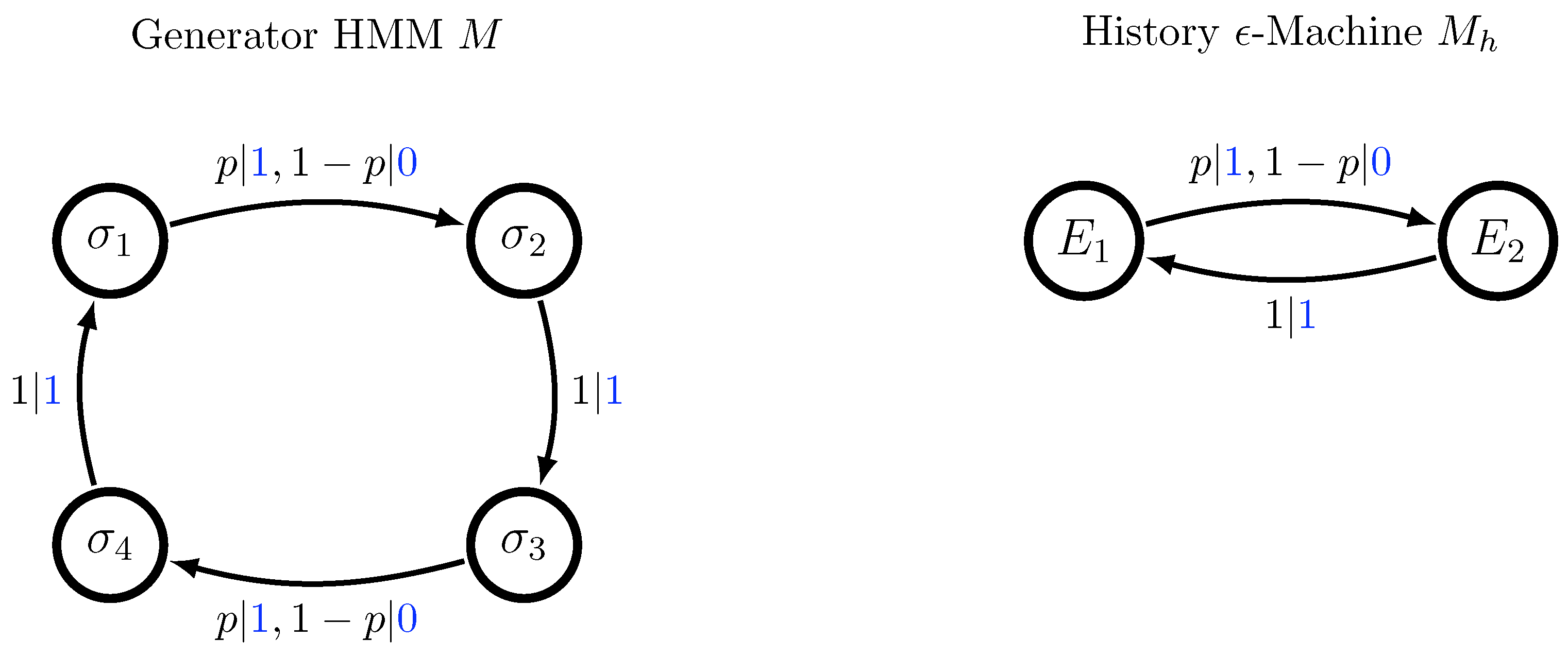
Example 2.

Alternating Biased Coins Machine

Figure 3 depicts a generating HMM M for the Alternating Biased Coins (ABC) Process. This process may be thought of as being generated by alternately flipping two coins with different biases $p\ne q$. The phase—p-bias on odd flips or p-bias on even flips—is chosen uniformly at random. M is again, by inspection, a generator $ϵ$-machine that is irreducible and unifilar with probabilistically distinct states. Therefore, by Theorem 1 below, the history $ϵ$-machine $M_h$ for the process $\mathcal{P}$ that M generates is again isomorphic to M. However, the Fischer cover for the sofic shift $\mathrm{supp}(\mathcal{P})$ is not isomorphic to M. The support of $\mathcal{P}$ is the full shift ${\mathcal{X}}^{\mathbb{Z}}$, so the Fischer cover consists of a single state transitioning to itself on both symbols 0 and 1.

In this simple example, the history $ϵ$-machine states can also be deduced directly, despite the fact that the generator M does not have a synchronizing word. If the initial state is $s_0={\sigma }_1$, then by the strong law of large numbers, the limiting fraction of 1s at odd time steps in finite-length past blocks ${\overleftarrow{x}}^t$ converges a.s. to q, whereas if the initial state is $s_0={\sigma }_2$, then the limiting fraction of 1s at odd time steps converges a.s. to p. Therefore, the initial state $s_0$ can be inferred a.s. from the complete past $\overleftarrow{x}$, so the process $\mathcal{P}$ is finitely characterized with two positive probability equivalence classes of infinite pasts $E_1$ and $E_2$, corresponding to the two states ${\sigma }_1$ and ${\sigma }_2$. Unlike the exact case, however, arguments like this do not generalize as easily to other nonexact generator $ϵ$-machines.

Example 3.

Nonminimal Noisy Period-2 Machine

Figure 4 depicts a nonminimal generating HMM M for the Noisy Period-2 (NP2) Process $\mathcal{P}$ in which 1s alternate with random symbols. M is again unifilar, but it does not have probabilistically distinct states and is, therefore, not a generator $ϵ$-machine. States ${\sigma }_1$ and ${\sigma }_3$ have the same probability distribution over future output sequences, as do states ${\sigma }_2$ and ${\sigma }_4$.

There are two positive probability equivalence classes of pasts $\overleftarrow{x}$ for the process $\mathcal{P}$, those containing 0s at a subset of the odd time steps, and those containing 0s at a subset of the even time steps. Those with 0s at odd time steps induce distributions over future output equivalent to that from states ${\sigma }_2$ and ${\sigma }_4$, while those with 0s at even time steps induce distributions over future output equivalent to that from states ${\sigma }_1$ and ${\sigma }_3$. Thus, the $ϵ$-machine for $\mathcal{P}$ consists of just two states, $E_1\sim \{{\sigma }_1,{\sigma }_3\}$ and $E_2\sim \{{\sigma }_2,{\sigma }_4\}$. In general, for a unifilar HMM without probabilistically distinct states, the $ϵ$-machine is formed by grouping together equivalent states in a similar fashion.

Example 4.

Simple Nonunifilar Source

Figure 5 depicts a generating HMM M known as the Simple Nonunifilar Source (SNS) [7]. The output process $\mathcal{P}$ generated by M consists of long sequences of 1s broken by isolated 0s. As its name indicates, M is nonunifilar, so it is not an $ϵ$-machine.

Symbol 0 is a synchronizing word for M, so all pasts $\overleftarrow{x}$ ending in a 0 induce the same probability distribution over future output sequences $\overrightarrow{x}$: Namely, the distribution over futures is given by starting M in the initial state $s_0={\sigma }_1$. However, since M is nonunifilar, an observer does not remain synchronized after seeing a 0. Any nontrivial past of the form $\overleftarrow{x}=\dots {01}^n$ induces the same distribution over the initial state $s_0$ as any other. However, for $n\ge 1$, there is some possibility of being in both ${\sigma }_1$ and ${\sigma }_2$ at time 0. A direct calculation shows that the distributions over $s_0$ and, hence, the distributions over future output sequences $\overrightarrow{x}$ are distinct for different values of n. Thus, since a.e. past $\overleftarrow{x}$ contains at least one 0, it follows that the process $\mathcal{P}$ has a countable collection of positive probability equivalence classes of pasts, comprising a set of full measure as follows: $\{E_n:n=0,1,2\dots \}$ where $E_n=\{\overleftarrow{x}=\dots {01}^n\}$. This leads to a countable-state history ϵ-machine $M_h$ as depicted on the right of Figure 5. We will not address countable-state machines further here, as other technical issues arise in this case. Conceptually, however, it is similar to the finite-state case and may be depicted graphically in an analogous fashion.

4. Equivalence

We will now show that the two $ϵ$-machine definitions—history and generator—are equivalent in the following sense:

• If $\mathcal{P}$ is the process generated by a generator $ϵ$-machine $M_g$, then $\mathcal{P}$ is finitely characterized and the history $ϵ$-machine $M_h(\mathcal{P})$ is isomorphic to $M_g$ as a hidden Markov model.
• If $\mathcal{P}$ is a finitely characterized, stationary, ergodic, finite-alphabet process, then the history $ϵ$-machine $M_h(\mathcal{P})$, when considered as a hidden Markov model, is also a generator $ϵ$-machine. Furthermore, the process ${\mathcal{P}}^{\prime }$ generated by $M_h$ is the same as the original process $\mathcal{P}$ from which the history machine was derived.

That is, there is a $1-1$ correspondence between finite-state generator $ϵ$-machines and finite-state history $ϵ$-machines. Every generator $ϵ$-machine is also a history $ϵ$-machine, for the same process $\mathcal{P}$ it generates. Every history $ϵ$-machine is also a generator $ϵ$-machine, for the same process $\mathcal{P}$ from which it was derived.

4.1. Generator $ϵ$-Machines Are History $ϵ$-Machines

In this section, we establish equivalence in the following direction:

Theorem 1.

If $\mathcal{P}=({\mathcal{X}}^{\mathbb{Z}},\mathbb{X},\mathbb{P})$ is the process generated by a generator ϵ-machine $M_g$, then $\mathcal{P}$ is finitely characterized and the history ϵ-machine $M_h(\mathcal{P})$ is isomorphic to $M_g$ as a hidden Markov model.

The key ideas in proving this theorem come from the study of synchronization to generator $ϵ$-machines [14,15]. In order to state these ideas precisely, however, we first need to introduce some terminology.

Let $M_g$ be a generator $ϵ$-machine, and let $\mathcal{P}=({\mathcal{X}}^{\mathbb{Z}},\mathbb{X},\mathbb{P})$ and $\tilde{\mathcal{P}}=({(\mathcal{X} \mathrm{x} \mathcal{S})}^{\mathbb{Z}},(\mathbb{X} \mathrm{x} \mathbb{S}),\tilde{\mathbb{P}})$ be the associated symbol and symbol-state processes generated by $M_g$ as in Section 3.2. Further, let the random variables $X_t:{(\mathcal{X} \mathrm{x} \mathcal{S})}^{\mathbb{Z}}\to \mathcal{X}$ and $S_t:{(\mathcal{X} \mathrm{x} \mathcal{S})}^{\mathbb{Z}}\to \mathcal{S}$ be the natural projections $X_t(\overleftrightarrow{x},\overleftrightarrow{s})=x_t$ and $S_t(\overleftrightarrow{x},\overleftrightarrow{s})=s_t$, and let ${\overrightarrow{X}}^t=X_0\dots X_{t-1}$ and ${\overleftarrow{X}}^t=X_{-t}\dots X_{-1}$.

The process language $Ł(\mathcal{P})$ is the set of words w of positive probability: $Ł(\mathcal{P})=\{w\in {\mathcal{X}}^{\ast }:\mathbb{P}(w)>0\}$. For a given word $w\in Ł(\mathcal{P})$, we define $\varphi (w)=\tilde{\mathbb{P}}(\mathcal{S}|w)$ to be an observer’s belief distribution as to the machine’s current state after observing the word w. Specifically, for a length-t word $w\in Ł(\mathcal{P})$, $\varphi (w)$ is a probability distribution over the machine states $\{{\sigma }_1,\cdots ,{\sigma }_N\}$ whose $i^{th}$ component is expressed as follows:

$$\begin{array}{cc}\hfill \varphi {(w)}_i& =\tilde{\mathbb{P}}(S_0={\sigma }_i|{\overleftarrow{X}}^t=w)\hfill \\ \hfill & =\tilde{\mathbb{P}}(S_0={\sigma }_i,{\overleftarrow{X}}^t=w)/\tilde{\mathbb{P}}({\overleftarrow{X}}^t=w).\hfill \end{array}$$

(25)

For a word $w\notin Ł(\mathcal{P})$ we will, by convention, take $\varphi (w)=\pi$.

For any word w, $\overline{\sigma }(w)$ is defined to be the most likely machine state at the current time given that the word w was just observed. That is, $\overline{\sigma }(w)={\sigma }_{i^{\ast }}$, where $i^{\ast }$ is defined by the relation $\varphi {(w)}_{i^{\ast }}={max}_i$$\varphi {(w)}_i$. In the case of a tie, $i^{\ast }$ is taken to be the lowest value of the index i maximizing the quantity $\varphi {(w)}_i$. Furthermore, $P(w)$ is defined to be the probability of the most likely state after observing w as follows:

$$\begin{array}{c}\hfill P(w)\equiv \varphi {(w)}_{i^{\ast }}.\end{array}$$

(26)

Furthermore, $Q(w)$ is defined to be the combined probability of all other states after observing w as follows:

$$\begin{array}{c}\hfill Q(w)\equiv \sum _{i\ne i^{\ast }}\varphi {(w)}_i=1-P(w).\end{array}$$

(27)

So, for example, if $\varphi (w)=(0.2,0.7,0.1)$, then $\overline{\sigma }(w)={\sigma }_2$, $P(w)=0.7$, and $Q(w)=0.3$.

The most recent t symbols are described by the block random variable ${\overleftarrow{X}}^t$, and so we define the corresponding random variables ${\Phi }_t=\varphi ({\overleftarrow{X}}^t)$, ${\overline{S}}_t=\overline{\sigma }({\overleftarrow{X}}^t)$, $P_t=P({\overleftarrow{X}}^t)$, and $Q_t=Q({\overleftarrow{X}}^t)$. Although the values depend only on the symbol sequence $\overleftrightarrow{x}$, formally, we think of ${\Phi }_t$, ${\overline{S}}_t$, $P_t$, and $Q_t$ as defined on the cross product space ${(\mathcal{X} \mathrm{x} \mathcal{S})}^{\mathbb{Z}}$. Their realizations are denoted with lowercase letters ${\varphi }_t$, ${\overline{s}}_t$, $p_t$, and $q_t$, so that for a given realization $(\overleftrightarrow{x},\overleftrightarrow{s})\in {(\mathcal{X} \mathrm{x} \mathcal{S})}^{\mathbb{Z}}$, ${\varphi }_t=\varphi ({\overleftarrow{x}}^t)$, ${\overline{s}}_t=\overline{\sigma }({\overleftarrow{x}}^t)$, $p_t=P({\overleftarrow{x}}^t)$, and $q_t=Q({\overleftarrow{x}}^t)$. The primary result we use is the following exponential decay bound on the quantity $Q_t$.

Lemma 1.

For any generator ϵ-machine $M_g$, there exist constants $K>0$ and $0<\alpha <1$ as follows:

$$\begin{array}{c}\hfill \tilde{\mathbb{P}}(Q_t>{\alpha }^t)\le K{\alpha }^t, for all t\in \mathbb{N}.\end{array}$$

(28)

Proof. 

This follows directly from the Exact Machine Synchronization Theorem of [15] and the Nonexact Machine Synchronization Theorem of [14] by stationarity (note that the notation used there differs slightly from that here by a time shift of length t. That is, $Q_t$ there refers to the observer’s doubt in $S_t$ given ${\overrightarrow{X}}^t$, instead of the observer’s doubt in $S_0$ given ${\overleftarrow{X}}^t$. Furthermore, L is used as a time index rather than t in those works). □

Essentially, this lemma says that after observing a block of t symbols, it is exponentially unlikely that an observer’s doubt $Q_t$ in the machine state will be more than exponentially small. Using the lemma, we now prove Theorem 1.

Proof. 

(Theorem 1) Let $M_g$ be a generator $ϵ$-machine with state set $\mathcal{S}=\{{\sigma }_1,\dots ,{\sigma }_N\}$ and stationary distribution $\pi =({\pi }_1,\dots ,{\pi }_N)$. Let $\mathcal{P}$ and $\tilde{\mathcal{P}}$ be the associated symbol and symbol-state processes generated by $M_g$. By Lemma 1 there exist constants $K>0$ and $0<\alpha <1$ such that $\tilde{\mathbb{P}}(Q_t>{\alpha }^t)\le K{\alpha }^t$, for all $t\in \mathbb{N}$. Let us define the following sets:

$$\begin{array}{cc}\hfill & V_t=\{(\overleftrightarrow{x},\overleftrightarrow{s}):q_t\le {\alpha }^t,s_0={\overline{s}}_t\},\hfill \\ \hfill & V_t^{\prime }=\{(\overleftrightarrow{x},\overleftrightarrow{s}):q_t\le {\alpha }^t,s_0\ne {\overline{s}}_t\},\hfill \\ \hfill & W_t=\{(\overleftrightarrow{x},\overleftrightarrow{s}):q_t>{\alpha }^t\}, \mathrm{and}\hfill \\ \hfill & U_t=W_t\cup V_t^{\prime }.\hfill \end{array}$$

Then, we obtain the following:

$$\begin{array}{cc}\hfill \tilde{\mathbb{P}}(U_t)& =\tilde{\mathbb{P}}(V_t^{\prime })+\tilde{\mathbb{P}}(W_t)\hfill \\ \hfill & \le {\alpha }^t+K{\alpha }^t\hfill \\ \hfill & =(K+1){\alpha }^t.\hfill \end{array}$$

So the following stands:

$$\begin{array}{c}\hfill \sum _{t=1}^{\infty }\tilde{\mathbb{P}}(U_t)\le \sum _{t=1}^{\infty }(K+1){\alpha }^t<\infty .\end{array}$$

Hence, by the Borel–Cantelli Lemma, $\tilde{\mathbb{P}}(U_t \mathrm{occurs} \mathrm{infinitely} \mathrm{often} )=0$. Or, equivalently, for $\tilde{\mathbb{P}}$ a.e. $(\overleftrightarrow{x},\overleftrightarrow{s})$, there exists $t_0\in \mathbb{N}$ such that $(\overleftrightarrow{x},\overleftrightarrow{s})\in V_t$ for all $t\ge t_0$. Now, we define the following:

$$\begin{array}{cc}\hfill C& =\{(\overleftrightarrow{x},\overleftrightarrow{s}): \mathrm{there} \mathrm{exists} t_0\in \mathbb{N} \mathrm{such} \mathrm{that} (\overleftrightarrow{x},\overleftrightarrow{s})\in V_t \mathrm{for} \mathrm{all} t\ge t_0\},\hfill \\ \hfill D_i& =\{(\overleftrightarrow{x},\overleftrightarrow{s}):s_0={\sigma }_i\}, \mathrm{and}\hfill \\ \hfill C_i& =C\cap D_i.\hfill \end{array}$$

According to the above discussion, $\tilde{\mathbb{P}}(C)=1$ and, clearly, $\tilde{\mathbb{P}}(D_i)={\pi }_i$. Thus, $\tilde{\mathbb{P}}(C_i)=\tilde{\mathbb{P}}(C\cap D_i)={\pi }_i$. Furthermore, by the convention for $\varphi (w),w\notin Ł(\mathcal{P})$, we know that for every $(\overleftrightarrow{x},\overleftrightarrow{s})\in C_i$, the corresponding symbol past $\overleftarrow{x}$ is nontrivial. So, the conditional probabilities $\mathbb{P}(w|{\overleftarrow{x}}^t)$ are well defined for each t.

Now, given any $(\overleftrightarrow{x},\overleftrightarrow{s})\in C_i$, we assume $t_0$ is sufficiently large so that for all $t\ge t_0$, $(\overleftrightarrow{x},\overleftrightarrow{s})\in V_t$. Then, for $t\ge t_0$, ${\overline{s}}_t={\sigma }_i$, and $q_t\le {\alpha }^t$. So, for any word $w\in {\mathcal{X}}^{\ast }$ and any $t\ge t_0$, the following stands:

$$\begin{array}{cc}\hfill |\mathbb{P}(w|& {\overleftarrow{x}}^t)-{\mathbf{P}}_{{\sigma }_i}(w)|\hfill \\ \hfill & =\left|\tilde{\mathbb{P}}({\overrightarrow{X}}^{|w|}=w|{\overleftarrow{X}}^t={\overleftarrow{x}}^t)-\tilde{\mathbb{P}}({\overrightarrow{X}}^{|w|}=w|S_0={\sigma }_i)\right|\hfill \\ \hfill & \stackrel{(\ast )}{=}\left|\left\{\sum _j\tilde{\mathbb{P}}({\overrightarrow{X}}^{|w|}=w|S_0={\sigma }_j)\tilde{\mathbb{P}}(S_0={\sigma }_j|{\overleftarrow{X}}^t={\overleftarrow{x}}^t)\right\}-\tilde{\mathbb{P}}({\overrightarrow{X}}^{|w|}=w|S_0={\sigma }_i)\right|\hfill \\ \hfill & =\left|\left\{\sum _{j\ne i}\tilde{\mathbb{P}}({\overrightarrow{X}}^{|w|}=w|S_0={\sigma }_j)\tilde{\mathbb{P}}(S_0={\sigma }_j|{\overleftarrow{X}}^t={\overleftarrow{x}}^t)\right\}-\left(1-\tilde{\mathbb{P}}(S_0={\sigma }_i|{\overleftarrow{X}}^t={\overleftarrow{x}}^t)\right)\tilde{\mathbb{P}}({\overrightarrow{X}}^{|w|}=w|S_0={\sigma }_i)\right|\hfill \\ \hfill & \le \left\{\sum _{j\ne i}\tilde{\mathbb{P}}({\overrightarrow{X}}^{|w|}=w|S_0={\sigma }_j)\tilde{\mathbb{P}}(S_0={\sigma }_j|{\overleftarrow{X}}^t={\overleftarrow{x}}^t)\right\}+\left(1-\tilde{\mathbb{P}}(S_0={\sigma }_i|{\overleftarrow{X}}^t={\overleftarrow{x}}^t)\right)\tilde{\mathbb{P}}({\overrightarrow{X}}^{|w|}=w|S_0={\sigma }_i)\hfill \\ \hfill & \le \left\{\sum _{j\ne i}\tilde{\mathbb{P}}(S_0={\sigma }_j|{\overleftarrow{X}}^t={\overleftarrow{x}}^t)\right\}+\left(1-\tilde{\mathbb{P}}(S_0={\sigma }_i|{\overleftarrow{X}}^t={\overleftarrow{x}}^t)\right)\hfill \\ \hfill & =2q_t\hfill \\ \hfill & \le 2{\alpha }^t.\hfill \end{array}$$

Step (*) follows from the fact that ${\overleftarrow{X}}^m$ and ${\overrightarrow{X}}^n$ are conditionally independent given $S_0$ for any $m,n\in \mathbb{N}$, by construction of the measure $\tilde{\mathbb{P}}$. Since $|\mathbb{P}(w|{\overleftarrow{x}}^t)-{\mathbf{P}}_{{\sigma }_i}(w)|\le 2{\alpha }^t$ for all $t\ge t_0$, we know ${lim}_{t\to \infty }\mathbb{P}(w|{\overleftarrow{x}}^t)={\mathbf{P}}_{{\sigma }_i}(w)$ exists. Since this holds for all $w\in {\mathcal{X}}^{\ast }$, we know $\overleftarrow{x}$ is regular and $\mathbf{P}(w|\overleftarrow{x})={\mathbf{P}}_{{\sigma }_i}(w)$ for all $w\in {\mathcal{X}}^{\ast }$.

Now, let us define equivalence classes $E_i$, $i=1,\dots ,N$, as follows:

$$\begin{array}{c}\hfill E_i=\{\overleftarrow{x}:\overleftarrow{x} \mathrm{is} \mathrm{regular} \mathrm{and} \mathbf{P}(w|\overleftarrow{x})={\mathbf{P}}_{{\sigma }_i}(w) \mathrm{for} \mathrm{all} w\in {\mathcal{X}}^{\ast }\}.\end{array}$$

Furthermore, also, for each $i=1,\dots ,N$ let the following be true:

$$\begin{array}{c}\hfill {\tilde{E}}_i=\{(\overleftrightarrow{x},\overleftrightarrow{s}):\overleftarrow{x}\in E_i\}.\end{array}$$

From the results from Appendix C we know that each equivalence class $E_i$ is measurable, so each set ${\tilde{E}}_i$ is also measurable with $\tilde{\mathbb{P}}({\tilde{E}}_i)=\mathbb{P}(E_i)$. Furthermore, for each i, $C_i\subseteq {\tilde{E}}_i$, so $\mathbb{P}(E_i)=\tilde{\mathbb{P}}({\tilde{E}}_i)\ge \tilde{\mathbb{P}}(C_i)={\pi }_i$. Since ${\sum }_{i=1}^N{\pi }_i=1$ and the equivalence classes $E_i,i=1,\dots ,N$, are all disjoint, it follows that $\mathbb{P}(E_i)={\pi }_i$ for each i, and ${\sum }_{i=1}^N\mathbb{P}(E_i)={\sum }_{i=1}^N{\pi }_i=1$. Hence, the process $\mathcal{P}$ is finitely characterized with positive probability equivalence classes ${\mathcal{E}}^{+}=\{E_1,\dots ,E_N\}$.

Moreover, the equivalence classes $\{E_1,\dots ,E_N\}$—the history $ϵ$-machine states—have a natural one-to-one correspondence with the states of the generating $ϵ$-machineas follows: $E_i\sim {\sigma }_i,i=1,\cdots ,N$. It remains only to verify that this bijection is also edge-preserving and, is thus, an isomorphism. Specifically, we must show the following:

• For each $i=1,\dots ,N$ and $x\in \mathcal{X}$, $\mathbf{P}(x|E_i)={\mathbf{P}}_{{\sigma }_i}(x)$.
• For all i and x with $\mathbf{P}(x|E_i)={\mathbf{P}}_{{\sigma }_i}(x)>0$, ${\delta }_h(E_i,x)\cong \delta ({\sigma }_i,x)$. That is, if ${\delta }_h(E_i,x)=E_j$ and $\delta ({\sigma }_i,x)={\sigma }_{j^{\prime }}$, then $j=j^{\prime }$.

Point 1 follows directly from the definition of $E_i$. To prove Point 2, take any i and x with $\mathbf{P}(x|E_i)={\mathbf{P}}_{{\sigma }_i}(x)>0$ and let ${\delta }_h(E_i,x)=E_j$ and $\delta ({\sigma }_i,x)={\sigma }_{j^{\prime }}$. Then, for any word $w\in {\mathcal{X}}^{\ast }$, we have the following:

(i)

$\mathbf{P}(xw|E_i)={\mathbf{P}}_{{\sigma }_i}(xw)$, by definition of the equivalence class $E_i$.

(ii)

$\mathbf{P}(xw|E_i)=\mathbf{P}(x|E_i)·\mathbf{P}(w|E_j)$, by Claim 11 in Appendix D.

(iii)

${\mathbf{P}}_{{\sigma }_i}(xw)={\mathbf{P}}_{{\sigma }_i}(x)·{\mathbf{P}}_{{\sigma }_{j^{\prime }}}(w)$, by Equation (10) applied to a unifilar HMM.

Since $\mathbf{P}(x|E_i)={\mathbf{P}}_{{\sigma }_i}(x)>0$, it follows that $\mathbf{P}(w|E_j)={\mathbf{P}}_{{\sigma }_{j^{\prime }}}(w)$. Since this holds for all $w\in {\mathcal{X}}^{\ast }$ and the states of the generator are probabilistically distinct, by assumption, it follows that $j=j^{\prime }$. □

Corollary 1.

Generator ϵ-machines are unique as follows: two generator ϵ-machines $M_{g_1}$ and $M_{g_2}$ that generate the same process $\mathcal{P}$ are isomorphic.

Proof. 

By Theorem 1, the two generator $ϵ$-machines are both isomorphic to the process’s history $ϵ$-machine $M_h(\mathcal{P})$ and, hence, isomorphic to each other. □

Remark 1.

Unlike history ϵ-machines that are unique by construction, generator ϵ-machines are not by definition unique. Furthermore, it is not a priori clear that they must be. Indeed, general HMMs are not unique. There are infinitely many nonisomorphic HMMs for any given process $\mathcal{P}$ generated by some HMM. Moreover, if either the unifilarity or probabilistically distinct states condition is removed from the definition of generator ϵ-machines, then uniqueness no longer holds. It is only when both of these properties are required together that one obtains uniqueness.

4.2. History $ϵ$-Machines Are Generator $ϵ$-Machines

In this section, we establish equivalence in the reverse direction as follows:

Theorem 2.

If $\mathcal{P}$ is a finitely characterized, stationary, ergodic, finite-alphabet process, then the history ϵ-machine $M_h(\mathcal{P})$, when considered as a hidden Markov model, is also a generator ϵ-machine. Furthermore, the process ${\mathcal{P}}^{\prime }$ generated by $M_h$ is the same as the original process $\mathcal{P}$ from which the history machine was derived.

Note that by Claim 17 in Appendix E we know that for any finitely characterized, stationary, ergodic, finite-alphabet process the history $ϵ$-machine $M_h(\mathcal{P})=({\mathcal{E}}^{+},\mathcal{X},\left\{T^{(x)}\right\})$ is a valid hidden Markov model. So, we need only show that this HMM has the three properties of a generator $ϵ$-machine—strongly connected graph, unifilar transitions, and probabilistically distinct states—and that the process ${\mathcal{P}}^{\prime }$ generated by this HMM is the same as $\mathcal{P}$. Unifilarity is immediate from the construction, but the other claims take more work and require several lemmas to establish. Throughout $\mu =({\mu }_1,\dots ,{\mu }_N)\equiv (\mathbb{P}(E_1),\dots ,\mathbb{P}(E_N))$, where ${\mathcal{E}}^{+}=\{E_1,\dots ,E_n\}$ is the set of positive probability equivalence classes for the process $\mathcal{P}$.

Lemma 2.

The distribution μ over equivalence-class states is stationary for the transition matrix $T={\sum }_{x\in \mathcal{X}}{T}^{(x)}$. That is, for any $1\le j\le N$, ${\mu }_j={\sum }_{i=1}^N{\mu }_i·T_{ij}$.

Proof. 

This follows directly from Claim 15 in Appendix E and the definition of the $T^{(x)}$ matrices. □

Lemma 3.

The graph G associated with the HMM $M_h=({\mathcal{E}}^{+},\mathcal{X},\left\{T^{(x)}\right\})$ consists entirely of disjoint strongly connected components. Each connected component of G is strongly connected.

Proof. 

It is equivalent to show that the graphical representation of the associated Markov chain with state set ${\mathcal{E}}^{+}$ and transition matrix T consists entirely of disjoint strongly connected components. However, this follows directly from the existence of a stationary distribution $\mu$ with ${\mu }_i=\mathbb{P}(E_i)>0$ for all i [31]. □

Lemma 4.

For any $E_i\in {\mathcal{E}}^{+}$ and $w\in {\mathcal{X}}^{\ast }$, $\mathbf{P}(w|E_i)={\mathbf{P}}_{E_i}(w)$, where ${\mathbf{P}}_{E_i}(w)\equiv {\parallel e_i{T}^{(w)}\parallel }_1$ is the probability of generating the word w starting in state $E_i$ of the HMM $M_h=({\mathcal{E}}^{+},\mathcal{X},\left\{T^{(x)}\right\})$ as defined in Section 3.2.

Proof. 

By construction, $M_h$ is a unifilar HMM, and its transition function $\delta$, as defined in Section 3.3, is the same as the transition function ${\delta }_h$ between equivalence classes of histories as defined in Equation (20). Moreover, we obtain by construction that for each $x\in \mathcal{X}$ and state $E_i$, ${\mathbf{P}}_{E_i}(x)=\mathbf{P}(x|E_i)$. The lemma essentially follows from these facts. We consider separately the two cases $\mathbf{P}(w|E_i)>0$ and $\mathbf{P}(w|E_i)=0$.

• Case (i)—$\mathbf{P}(w|E_i)>0$. Let $w=w_0\dots w_{l-1}$ be a word of length $l\ge 1$ with $\mathbf{P}(w|E_i)>0$. By Claim 12 in Appendix D and the ensuing remark, we know that the equivalence classes $s_0=E_i$, $s_1={\delta }_h(s_0,w_0),\dots ,s_l={\delta }_h(s_{l-1},w_{l-1})$ are well defined and the following stands:

  $$\begin{array}{c}\hfill \mathbf{P}(w|E_i)=\prod _{t=0}^{l-1}\mathbf{P}(w_t|s_t).\end{array}$$
  Since ${\delta }_h\cong \delta$, we see that there is an allowed state path s in the HMM $M_h$—namely, $s=s_1,\dots ,s_l$—such that the word w can be generated following s from the initial state $E_i$. It follows that ${\mathbf{P}}_{E_i}(w)>0$ and is given by Equation (15) as follows:

  $$\begin{array}{c}\hfill {\mathbf{P}}_{E_i}(w)=\prod _{t=0}^{l-1}{\mathbf{P}}_{s_t}(w_t)=\prod _{t=0}^{l-1}\mathbf{P}(w_t|s_t).\end{array}$$
• Case (ii)—$\mathbf{P}(w|E_i)=0$. Let $w=w_0\dots w_{l-1}$ be a word of length $l\ge 1$ with $\mathbf{P}(w|E_i)=0$. For $0\le m\le l-1$, define $w^m=w_0\dots w_{m-1}$ ($w^0$ is the null word $\lambda$). Take the largest integer $m\in \{0,\dots ,l-1\}$ such that $\mathbf{P}(w^m|E_i)>0$. By convention, we take $\mathbf{P}(\lambda |E_i)=1$ for all i, so there is always some such m. A similar analysis to above then shows that the equivalence classes $s_0,\dots ,s_m$ defined by $s_0=E_i$, $s_{t+1}={\delta }_h(s_t,w_t)$ are well defined and the following stands:

  $$\begin{array}{c}\hfill \mathbf{P}(w^{m+1}|E_i)=\prod _{t=0}^m\mathbf{P}(w_t|s_t)={\mathbf{P}}_{E_i}(w^{m+1}).\end{array}$$
  By our choice of m, $\mathbf{P}(w^{m+1}|E_i)=0$, so ${\mathbf{P}}_{E_i}(w^{m+1})=0$ as well. It follows that ${\mathbf{P}}_{E_i}(w)=0$, since $w^{m+1}$ is a prefix of w.

□

Lemma 5.

For any $w\in {\mathcal{X}}^{\ast }$, $\mathbb{P}(w)=\parallel \mu T^{(w)}{\parallel }_1$.

Proof. 

Let $E_{i,w}\equiv \{\overleftrightarrow{x}:{\overrightarrow{x}}^{|w|}=w,\overleftarrow{x}\in E_i\}$. Claim 14 of Appendix D shows that each $E_{i,w}$ is an $\mathbb{X}$-measurable set with $\mathbb{P}(E_{i,w})=\mathbb{P}(E_i)·\mathbf{P}(w|E_i)$. Since the $E_i$s are disjoint sets with probabilities summing to 1, it follows that $\mathbb{P}(w)={\sum }_{i=1}^N\mathbb{P}(E_{i,w})$ for each $w\in {\mathcal{X}}^{\ast }$. Thus, applying Lemma 4, for any $w\in {\mathcal{X}}^{\ast }$ we have the following:

$$\begin{array}{cc}\hfill \mathbb{P}(w)& =\sum _{i=1}^N\mathbb{P}(E_{i,w})\hfill \\ \hfill & =\sum _{i=1}^N\mathbb{P}(E_i)·\mathbf{P}(w|E_i)\hfill \\ \hfill & =\sum _{i=1}^N{\mu }_i{\parallel e_i{T}^{(w)}\parallel }_1\hfill \\ \hfill & =\parallel \mu T^{(w)}{\parallel }_1.\hfill \end{array}$$

□

Proof. 

(Theorem 2)

• Unifilarity: As mentioned above, this is immediate from the history $ϵ$-machine construction.
• Probabilistically Distinct States: Take any i and j with $i\ne j$. By construction of the equivalence classes there exists some word $w\in {\mathcal{X}}^{\ast }$ such that $\mathbf{P}(w|E_i)\ne \mathbf{P}(w|E_j)$. However, by Lemma 4, $\mathbf{P}(w|E_i)={\mathbf{P}}_{E_i}(w)$ and $\mathbf{P}(w|E_j)={\mathbf{P}}_{E_j}(w)$. Hence, ${\mathbf{P}}_{E_i}(w)\ne {\mathbf{P}}_{E_j}(w)$, so the states $E_i$ and $E_j$ of the HMM $M_h=({\mathcal{E}}^{+},\mathcal{X},\left\{T^{(x)}\right\})$ are probabilistically distinct. Since this holds for all $i\ne j$, $M_h$ has probabilistically distinct states.
• Strongly Connected Graph: By Lemma 3, we know the graph G associated with the HMM $M_h$ consists of one or more connected components $C_1,\dots ,C_n$, each of which is strongly connected. Assume that there is more than one of these strongly connected components: $n\ge 2$. By Points 1 and 2 above we know that each component $C_k$ defines a generator $ϵ$-machine. If two of these components $C_k$ and $C_j$ were isomorphic via a function $f:C_k$ states $\to C_j$ states, then for states $E_i\in C_k$ and $E_l\in C_j$ with $f(E_i)=E_l$, we would have ${\mathbf{P}}_{E_i}(w)={\mathbf{P}}_{E_l}(w)$ for all $w\in {\mathcal{X}}^{\ast }$. By Lemma 4, however, this implies $\mathbf{P}(w|E_i)=\mathbf{P}(w|E_l)$ for all $w\in {\mathcal{X}}^{\ast }$ as well, which contradicts the fact that $E_i$ and $E_l$ are distinct equivalence classes. Hence, no two of the components $C_k,k=1,\dots ,n$, can be isomorphic. By Corollary 1, this implies that the stationary processes ${\mathcal{P}}^k,k=1,\dots ,n$, generated by each of the generator $ϵ$-machine components, are all distinct. However, by a block diagonalization argument, it follows from Lemma 5 that $\mathcal{P}={\sum }_{k=1}^n{\mu }^k·{\mathcal{P}}^k$, where ${\mu }^k={\sum }_{\{i:E_i\in C_k\}}{\mu }_i$. That is, for any word $w\in {\mathcal{X}}^{\ast }$, we have the following:

  $$\begin{array}{cc}\hfill \mathbb{P}(w)& =\sum _{k=1}^n{\mu }^k·{\mathbb{P}}^k(w)\hfill \\ \hfill & =\sum _{k=1}^n{\mu }^k·{\parallel {\rho }^k{T}^{k,(w)}\parallel }_1,\hfill \end{array}$$

  where ${\rho }^k$ and $T^{k,(w)}$ are, respectively, the stationary state distribution and w-transition matrix for the generator $ϵ$-machine of component $C_k$. Since the ${\mathcal{P}}^k$s are all distinct, this implies that the process $\mathcal{P}$ cannot be ergodic, which is a contradiction. Hence, there can only be one strongly connected component $C_1$—the whole graph is strongly connected.
• Equivalence of $\mathcal{P}$ and ${\mathcal{P}}^{\prime }$: Since the graph of the HMM $M_h=({\mathcal{E}}^{+},\mathcal{X},\left\{T^{(x)}\right\})$ is strongly connected there is a unique stationary distribution $\pi$ over the states satisfying $\pi =\pi T$. However, we already know the distribution $\mu$ is stationary. Hence, $\pi =\mu$. By definition, the word probabilities ${\mathbb{P}}^{\prime }(w)$ for the process ${\mathcal{P}}^{\prime }$ generated by this HMM are ${\mathbb{P}}^{\prime }(w)={\parallel \pi T^{(w)}\parallel }_1,w\in {\mathcal{X}}^{\ast }$. However, by Lemma 5, we have also $\mathbb{P}(w)=\parallel \mu T^{(w)}{\parallel }_1={\parallel \pi T^{(w)}\parallel }_1$ for each $w\in {\mathcal{X}}^{\ast }$. Hence, $\mathbb{P}(w)={\mathbb{P}}^{\prime }(w)$ for all $w\in {\mathcal{X}}^{\ast }$, so $\mathcal{P}$ and ${\mathcal{P}}^{\prime }$ are the same process.

□

5. Conclusions

We have demonstrated the equivalence of finite-state history and generator $ϵ$-machines. This is not a new idea. However, a formal treatment was absent until quite recently and, while the rigorous development of $ϵ$-machines in [16] also implies equivalence, the proofs given here, especially for Theorem 1, are more direct and provide improved intuition.

The key step in proving the equivalence, at least the new approach used for Theorem 1, comes directly from recent bounds on synchronization rates for finite-state generator $ϵ$-machines. To generalize the equivalence to larger model classes, such as machines with a countably infinite number of states, it therefore seems reasonable that one should first deduce and apply similar synchronization results for countable-state generators. Unfortunately, for countable-state generators, synchronization can be much more difficult and exponential decay rates as in Lemma 1 no longer always hold. Thus, it is unclear whether equivalence in the countable-state case also always holds. Nevertheless, the results in [16] do indicate equivalence holds for countable-state machines if the entropy in the stationary distribution $H\left[\pi \right]$ is finite, which it often is.

References

1. Crutchfield, J.P.; Young, K. Inferring statistical complexity. Phys. Rev. Let. 1989, 63, 105–108. [Google Scholar] [CrossRef]
2. Crutchfield, J.P.; Feldman, D.P. Statistical complexity of simple one-dimensional spin systems. Phys. Rev. E 1997, 55, 1239R–1243R. [Google Scholar] [CrossRef]
3. Varn, D.P.; Canright, G.S.; Crutchfield, J.P. Discovering planar disorder in close-packed structures from X-ray diffraction: Beyond the fault model. Phys. Rev. B 2002, 66, 174110. [Google Scholar] [CrossRef]
4. Varn, D.P.; Crutchfield, J.P. From finite to infinite range order via annealing: The causal architecture of deformation faulting in annealed close-packed crystals. Phys. Lett. A 2004, 234, 299–307. [Google Scholar] [CrossRef]
5. Still, S.; Crutchfield, J.P.; Ellison, C.J. Optimal causal inference: Estimating stored information and approximating causal architecture. Chaos Interdiscip. J. Nonlinear Sci. 2010, 20, 037111. [Google Scholar] [CrossRef] [PubMed]
6. Li, C.-B.; Yang, H.; Komatsuzaki, T. Multiscale complex network of protein conformational fluctuations in single-molecule time series. Proc. Natl. Acad. Sci. USA 2008, 105, 536–541. [Google Scholar] [CrossRef]
7. Crutchfield, J.P. The calculi of emergence: Computation, dynamics, and induction. Phys. D 1994, 75, 11–54. [Google Scholar] [CrossRef]
8. Upper, D.R. Theory and Algorithms for Hidden Markov Models and Generalized Hidden Markov Models. Ph.D. Thesis, University of California, Berkeley, CA, USA, 1997. [Google Scholar]
9. Shalizi, C.R.; Crutchfield, J.P. Computational mechanics: Pattern and prediction, structure and simplicity. J. Stat. Phys. 2001, 104, 817–879. [Google Scholar] [CrossRef]
10. Ay, N.; Crutchfield, J.P. Reductions of hidden information sources. J. Stat. Phys. 2005, 210, 659–684. [Google Scholar] [CrossRef]
11. Löhr, W. Predictive Models and Generative Complexity. J. Syst. Sci. Complex 2009, 25, 30–45. [Google Scholar] [CrossRef]
12. Löhr, W.; Ay, N. Non-sufficient Memories That Are Sufficient for Prediction. In Complex 2009: First International Conference, Shanghai, China, 23–25 February 2009; Zhou, J., Ed.; LNICST 4; Springer: Berlin/Heidelberg, Germany, 2009; pp. 265–276. [Google Scholar]
13. Löhr, W. Properties of the Statistical Complexity Functional and Partially Deterministic HMMs. Entropy 2009, 11, 385–401. [Google Scholar] [CrossRef]
14. Travers, N.F.; Crutchfield, J.P. Asymptotic synchronization for finite-state sources. J. Stat. Phys. 2011, 145, 1202–1223. [Google Scholar] [CrossRef]
15. Travers, N.F.; Crutchfield, J.P. Exact synchronization for finite-state sources. J. Stat. Phys. 2011, 145, 1181–1201. [Google Scholar] [CrossRef]
16. Löhr, W. Models of Discrete Time Stochastic Processes and Associated Complexity Measures. PhD Thesis, Max Planck Institute for Mathematics in the Sciences, Leipzig, Germany, 2010. [Google Scholar]
17. Boyle, M.; Petersen, K. Hidden Markov processes in the context of symbolic dynamics. arXiv 2009, arXiv:0907.1858. [Google Scholar]
18. Weiss, B. Subshifts of finite type and sofic systems. Monatsh. Math. 1973, 77, 462–474. [Google Scholar] [CrossRef]
19. Hopcroft, J.E.; Ullman, J.D. Introduction to Automata Theory, Languages, and Computation; Addison-Wesley: Reading, UK, 1979. [Google Scholar]
20. Fischer, R. Sofic systems and graphs. Monatsh. Math. 1975, 80, 179–186. [Google Scholar] [CrossRef]
21. Boyle, M.; Kitchens, B.; Marcus, B. A note on minimal covers for sofic systems. Proc. AMS 1985, 95, 403–411. [Google Scholar] [CrossRef]
22. Lind, D.; Marcus, B. An Introduction to Symbolic Dynamics and Coding; Cambridge University Press: New York, NY, USA, 1995. [Google Scholar]
23. Kitchens, B.; Tuncel, S. Finitary measures for subshifts of finite type and sofic systems. Mem. AMS 1985, 58, 338. [Google Scholar] [CrossRef]
24. Harris, T.E. On chains of infinite order. Pacific J. Math. 1955, 5, 707–724. [Google Scholar] [CrossRef]
25. Keane, M. Strongly mixing g-measures. Invent. Math. 1972, 16, 309–324. [Google Scholar] [CrossRef]
26. Bramson, M.; Kalikow, S. Nonuniqueness in g-functions. Isr. J. Math. 1993, 84, 153–160. [Google Scholar] [CrossRef]
27. Stenflo, Ö. Uniqueness in g-measures. Nonlinearity 2003, 16, 403–410. [Google Scholar] [CrossRef]
28. Krieger, W.; Weiss, B. On g measures in symbolic dynamics. Isr. J. Math 2010, 176, 1–27. [Google Scholar] [CrossRef]
29. Rabiner, L.R. A tutorial on hidden Markov models and selected applications in speech recognition. IEEE Proc. 1989, 77, 257. [Google Scholar] [CrossRef]
30. Ephraim, Y.; Merhav, N. Hidden Markov processes. IEEE Trans. Inf. Theory 2002, 48, 1518–1569. [Google Scholar] [CrossRef]
31. Levin, D.; Peres, Y.; Wilmer, E.L. Markov Chains and Mixing Times; American Mathematical Society: Providence, RI, USA, 2006. [Google Scholar]
32. Durrett, R. Probability: Theory and Examples, 2nd ed.; Wadsworth Publishing Company: Pacific Grove, CA, USA, 1995. [Google Scholar]
Figure 1. A hidden Markov model (the ϵ -machine) for the Even Process. The HMM has two internal states S = { σ 1 , σ 2 } , a two-symbol alphabet X = { 0 , 1 } , and a single parameter p ( 0 , 1 ) that controls the transition probabilities.
Symmetry 17 00078 g001
Figure 2. The Even Machine M (left) and associated history ϵ -machine M h (right) for the process P generated by M. p ( 0 , 1 ) is a parameter.
Symmetry 17 00078 g002
Figure 3. The Alternating Biased Coins (ABC) Machine M (left) and associated history ϵ -machine M h (right) for the process P n generated by M. p , q ( 0 , 1 ) are parameters, p q .
Symmetry 17 00078 g003
Figure 4. A nonminimal generating HMM M for the Noisy Period-2 (NP2) Process (left), and the associated history ϵ -machine M h for this process (right). p ( 0 , 1 ) is a parameter.
Symmetry 17 00078 g004
Figure 5. The Simple Nonunifilar Source (SNS) M (left) and associated history ϵ -machine M h (right) for the process P generated by M. In the history ϵ -machine, q n + p n = 1 for each n N , and ( q n ) n N is an increasing sequence defined by the following: q n = ( 1 q ) · ( 1 p ) m = 0 n 1 p m q n 1 m / p n + ( 1 p ) m = 0 n 1 p m q n 1 m .
Symmetry 17 00078 g005
Disclaimer/Publisher’s Note: The statements, opinions and data contained in all publications are solely those of the individual author(s) and contributor(s) and not of MDPI and/or the editor(s). MDPI and/or the editor(s) disclaim responsibility for any injury to people or property resulting from any ideas, methods, instructions or products referred to in the content.