A Robust EfficientNetV2-S Classifier for Predicting Acute Lymphoblastic Leukemia Based on Cross Validation

Abstract

This research addresses the challenges of early detection of Acute Lymphoblastic Leukemia (ALL), a life-threatening blood cancer particularly prevalent in children. Manual diagnosis of ALL is often error-prone, time-consuming, and reliant on expert interpretation, leading to delays in treatment. This study proposes an automated binary classification model based on the EfficientNetV2-S architecture to overcome these limitations, enhanced with 5-fold cross-validation (5KCV) for robust performance. A novel aspect of this research lies in leveraging the symmetry concepts of symmetric and asymmetric patterns within the microscopic imagery of white blood cells. Symmetry plays a critical role in distinguishing typical cellular structures (symmetric) from the abnormal morphological patterns (asymmetric) characteristic of ALL. By integrating insights from generative modeling techniques, the study explores how asymmetric distortions in cellular structures can serve as key markers for disease classification. The EfficientNetV2-S model was trained and validated using the normalized C-NMC_Leukemia dataset, achieving exceptional metrics: 97.34% accuracy, recall, precision, specificity, and F1-score. Comparative analysis showed the model outperforms recent classifiers, making it highly effective for distinguishing abnormal white blood cells. This approach accelerates diagnosis, reduces costs, and improves patient outcomes, offering a transformative tool for early ALL detection and treatment planning.

1. Introduction

Blood plays a critical role in the human body by carrying out various vital functions necessary for life. It flows through the circulatory system, delivering oxygen and important nutrients to tissues and organs, removing waste products, and performing essential tasks in the immune system. Additionally, blood helps regulate body temperature, ensuring optimal functioning. Bone marrow is a soft tissue found inside the hollow sections of bones, predominantly in the hip and thigh bones. It is essential for the body’s production of blood cells [1]. The blood is composed of [1,2,3] plasma (55% of blood volume), red blood cells (RBCs) (45%), white blood cells (WBCs) (<1%), and platelets.

Leukemia is a blood cancer originating in the bone marrow, leading to the excessive production of abnormal WBCs that disrupt normal blood cell production. It affects both adults and children, causing health issues due to dysfunctional WBCs outnumbering healthy cells. Early detection is crucial for effective treatment, as its symptoms resemble other illnesses. Leukemia is classified into four main types [4,5,6]. ALL affects lymphoid cells and tends to progress quickly in children, but it can also occur in adults. Acute Myeloid Leukemia (AML) affects myeloid cells and usually advances rapidly in adults but can also appear in children. Chronic Lymphocytic Leukemia (CLL) targets lymphoid cells, progresses slowly, and is mainly found in older adults. Chronic Myeloid Leukemia (CML) affects myeloid cells, progresses gradually, and is more common in adults.

ALL is a blood and bone marrow cancer marked by the rapid proliferation of immature white blood cells [7,8]. It is a severe disease that predominantly affects children, accounting for 25% of childhood cancer cases, but it can also occur in adults. Among individuals under 20, ALL represents 74% of leukemia cases. Children under 14 have a high five-year survival rate of 91%, while teenagers aged 15–20 have a slightly lower rate of 75%. However, adult recovery rates five years after diagnosis are significantly lower, ranging from 20% to 35% [9]. Early diagnosis and treatment improve survival outcomes. ALL is divided into three subtypes—L1, L2, and L3—based on cell structure, categorized by the French American British (FAB) system [10,11,12].

Acute Lymphoblastic Leukemia (ALL) symptoms develop rapidly. They may include fatigue, frequent infections, fever, easy bruising or bleeding, bone or joint pain, swollen lymph nodes, breathing difficulties, unexplained weight loss, and night sweats. Diagnosis involves a combination of methods, each with strengths and limitations [13]:

1. Blood Tests: A complete blood count (CBC) measures levels of RBCs, WBCs, and platelets, and a blood smear examines cells microscopically. While these tests can indicate abnormalities, they cannot confirm ALL and require further testing [14,15].

2. Bone Marrow Examination: Bone marrow aspiration (removing liquid marrow) and biopsy (removing a tissue sample) are definitive but invasive procedures with potential risks like bleeding and infection [16].

3. Imaging Tests: X-rays, CT scans, and MRIs assess organ involvement and complications but cannot replace bone marrow tests for a definitive diagnosis [17,18].

Diagnosing ALL can be difficult because early or minimal signs of the disease may not be picked up in initial tests. There are also similarities between ALL and various infections or other bone marrow disorders. Interpreting complex tests such as flow cytometry and genetic testing require highly skilled hematologists. In resource-limited settings, advanced diagnostic methods may not be available, and delays in getting results from genetic and molecular tests can slow down timely diagnosis and treatment.

To address the limitations of traditional diagnostic methods, automating the analysis of blood and bone marrow samples using modern machine learning (ML) techniques, such as deep learning (DL) networks, has become essential. Convolutional Neural Networks (CNNs) are particularly effective in early detection of Acute Lymphoblastic Leukemia (ALL), as they can independently learn spatial features from input images. By employing backpropagation, CNNs refine parameters and weights to improve accuracy. Additionally, segmentation techniques isolate white blood cells (WBCs) in blood images, enabling precise analysis through feature extraction. CNNs have proven highly effective in medical applications, accurately identifying diseases and distinguishing normal from abnormal blood cells [19].

The primary goal of this research is to create a strong, optimized model using the EfficientNetV2-S model for classifying ALL into two categories: ALL or Healthy. A unique feature of this research focuses on utilizing symmetrical principles in symmetric and asymmetric patterns found in microscopic images of white blood cells. Symmetry is essential for differentiating typical cell structures, which are symmetric, from the abnormal morphological characteristics, which are asymmetric, typically associated with Acute Lymphoblastic Leukemia (ALL). By incorporating knowledge from generative modeling methods, the study examines how asymmetric alterations in cell structures can act as significant indicators for classifying the disease. The research utilized the 5KCV technique to improve the efficiency of the EfficientNetV2-S model. This method allowed for effective fine-tuning of the model parameters. The proposed model is crucial for assisting hematologists in the early identification of ALL, leading to better patient outcomes and a quicker, more cost-efficient diagnostic process. It helps reduce both the time taken and the expenses incurred by patients. An experiment was carried out on the C-NMC_Leukemia dataset specifically for ALL diagnoses. The dataset underwent initial processing steps, such as resizing and standardization. It was split into 70% for training and validation and 30% for testing. Comparative analyses with other models such as EfficientNet-B1, EfficientNet-B3, InceptionV3, and Xception revealed that the EfficientNetV2-S model achieved exceptional performance metrics, including an average recall, accuracy, specificity, and F1-score of 97.34%, along with a precision of 97.34%. With proper adjustments, the assessment emphasized that the proposed model surpassed existing models, demonstrating its effectiveness in detecting ALL. Compared to traditional classification systems, the exceptional performance of our proposed model was evident. Our classifier’s evaluation emphasized our Methodology’s potential, demonstrating effectiveness in accurately identifying ALL. Here are some highlights of the effects our research has had:

• We successfully detected ALL by combining the 5KCV method with the EfficientNetV2-S approach. They created a robust customized classifier to predict the presence of ALL using the C-NMC_Leukemia dataset, providing a ground-breaking solution in this field.
• To our knowledge, the EfficientNetV2-S approach is being used for the first time to detect ALL.
• A comprehensive statistical analysis was conducted using all methods.
• The proposed model, which integrated the 5KCV method with the Efficient-NetV2-S, was meticulously designed to uphold a harmonious equilibrium and mitigate issues related to overfitting.
• Our model has shown outstanding precision in identifying ALL while using minimal time and resources.
• Utilizing our proposed model from the beginning has displayed potential in quickly identifying ALL, proving to be a valuable tool in pathology by assisting in prompt and tailored patient care.
• An optimized model we designed delivered impressive results, boasting average recall, accuracy, specificity, and F1-score of 97.34%, as well as a precision of 97.34%.

The paper’s structure overview is as follows: Section 2 reviews ALL diagnostic systems. Section 3 covers Pre-processing procedures for the C-NMC_Leukemia dataset and Methodology. Section 4 shows the experimental results of the proposed model. Section 5 concludes with remarks.

2. Literature Review

Artificial Intelligence (AI), ML, and DL are rising in leukemia diagnosis research as potent aids. AI algorithms are being developed to scrutinize intricate data collected from blood tests, bone marrow biopsies, and imaging examinations. These technological advancements can support the early identification and categorization of different types of leukemia and forecast treatment outcomes by recognizing distinctive patterns and irregularities that might go unnoticed through conventional techniques. As a result, there is the potential for quicker and more precise diagnoses. For example, Mondal et al. [20] identified ALL using CNN models. The researchers investigated a combination of deep CNN models with varied weights to boost the accuracy of an ALL-cell classifier. Different techniques like data augmentations and pre-processing methods were utilized to improve the overall performance and adaptability of the network. The C-NMC-2019 ALL dataset was employed as their model’s training and evaluation dataset. The developed model demonstrated results, including an Area Under the Curve (AUC) of 94.8%, a balanced accuracy of 88.3%, and a weighted F1-score of 89.7%.

R. Khandekar et al. [21] created an automated system powered by AI to detect blast cells. This system utilized images of small blood smears to predict leukemic cells. They incorporated the You Only Look Once (YOLO) algorithm, specifically its fourth version, to categorize and detect cells. The cells were classified into healthy cells (HEM) and blast cells (ALL), treating the task as a binary problem. The Object Detection algorithm was trained and evaluated using images from the ALL_IDB1 and C_NMC_2019 datasets. The ALL_IDB1 dataset demonstrated a mean average precision (mAP) of 96.06%, while the C_NMC_2019 dataset achieved a high mAP of 98.7%.

Almadhor et al. [22] employed various ML algorithms, including the naive Bayes (NB), K-nearest neighbor (KNN), random forest (RF), and support vector machine (SVM) to develop an ensembled automated forecasting technique. They concentrated on the C-NMC leukemia dataset obtained from Kaggle, which comprises healthy and cancer cell groupings. Results revealed that SVM outperformed the other models, attaining an accuracy level of 90%.

Kasani et al. [23] introduced a unified DL model to classify leukemic B-lymphoblasts. They utilized data augmentation techniques to create additional training samples to address the limited dataset size. Implementing transfer learning expedited the training process and improved the network’s performance, leading to a reliable and accurate DL system. Their proposed approach achieved an accuracy rate of 96.58% on the test dataset for diagnosing Leukemic B-lymphoblasts.

Liu et al. [24] proposed and introduced a network called the ternary stream-driven weakly supervised data augmentation classification network (WT-DFN) to support the early and accurate diagnosis of Acute Lymphoblastic Leukemia (ALL). This method aimed to identify lymphoblasts in detail using microscopic images of peripheral blood smears. For each training image, they created attention maps through weakly supervised learning, highlighting the critical areas to focus on. They then generated two additional streams using attention cropping and attention erasing techniques, allowing them to capture fine details that distinguish features effectively. The model was tested on the C-NMC database, achieving an impressive accuracy rate of about 91.90%.

Sulaiman et al. [25] proposed a novel method, ResRandSVM, to detect ALL blood smear images by leveraging advanced deep feature extraction techniques. This approach utilized seven different Deep Learning (DL) models to extract features from the blood smear images, namely: ResNet152, VGG16, DenseNet121, MobileNetV2, InceptionV3, EfficientNetB0, and ResNet50. Following the feature extraction process, three feature selection methods were employed to identify crucial features: analysis of variance (ANOVA), principal component analysis (PCA), and RF. Subsequently, the selected feature map was input into four distinct classifiers—Adaboost, Support Vector Machine (SVM), Artificial Neural Network (ANN), and Naive Bayes (NB) models—to categorize the images into either leukemia or normal images. The most successful combination of models was determined to be utilizing ResNet50 for feature extraction, RF for feature selection, and SVM as the classifier, resulting in an accuracy of 90%, a precision of 90.2%, a recall of 95.7%, and an F1-score of 92.9%. The dataset used for this research was the C-NMC database, split into an 80% training set and a 20% test set.

The limitations of the previous studies are as follows:

• The researchers discussed earlier research concentrated on metrics such as accuracy, precision, recall, and F1 score, but they overlooked the assessment of results using statistical confidence intervals. In contrast, we have effectively utilized statistical methods to examine and compare the outcomes from different DL approaches by exploring confidence intervals, underscoring our Methodology’s unique advantage.
• The researchers from the earlier discussed study did not perform an ablation analysis. In contrast, we undertook this analysis to understand how specific components or features of our proposed model influence performance by methodically eliminating or altering them and monitoring the resultant effects.

3. Materials and Methods

3.1. Materials

The proposed research model utilized the C-NMC_Leukemia dataset [26] to make predictions regarding ALL cells. This dataset was supplied by the Cancer Imaging Archive (TCIA) for the ALL Disease Diagnostics Competition, which the Cancer Program of the National Cancer Institute in the United States supports. The primary objective of TCIA is to advance computer-aided technologies. The competition aims to develop automated systems distinguishing between blood cells affected by leukemia and normal, healthy cells. The dataset comprises images of white blood cells captured under a microscope. These images are classified into normal (healthy) and leukemic (cancerous) cells. They have been gathered from various patients under different conditions to ensure diversity and consistency. The images are usually stored separately based on their classification (normal or cancerous) and are accompanied by corresponding labels for training and evaluation purposes. These images are of high quality and contain essential details crucial for accurate diagnostics. Some images may include additional information such as magnification levels, staining techniques, and de-identified patient data. Overall, the dataset contains 10,661 cell images obtained from 76 patients.

Table 1. The classes’ distribution of the C-NMC_Leukemia dataset.

Class	Image Count
Healthy	3389
ALL	7272
10,661

shows 7272 images from 47 patients diagnosed with ALL, while the remaining 3389 images are from 26 healthy individuals. This extensive C-NMC dataset provides a significant number of valuable images for the development of a robust diagnostic classifier for ALL. All images in the dataset are in RGB color format with a resolution of 450 × 450 pixels. Figure 1 shows different samples of ALL and health images from the C-NMC dataset.

During the initial phase of the C-NMC_Leukemia test set, 1867 cells were identified. Among them, 1219 malignant cells were identified in 13 subjects, and 648 healthy cells were identified in 15. In the final phase of the test set, 2586 cells had not yet been labeled, collected from 17 subjects. Expert oncologists have identified single-cell images of malignant and benign lymphocytes, which can be accessed in dedicated folders.

Table 2. The division of the C-NMC_Leukemia dataset.

Set	Healthy	ALL
Training	1691	5573
Test	1698	1699
Total	3389	7272

shows the division of the C-NMC_Leukemia dataset into training and test sets.

3.2. Methodology

We combined the 5KCV method with the EfficientNetV2-S to classify ALL. The EfficientNetV2-S model was utilized for the binary classification of ALL, while 5KCV was employed to evaluate the model’s performance comprehensively. In 5KCV, the data is divided into five subsets. The model is trained on four subsets and tested on the fifth. This process is repeated five times so that each subset can be the test set. Following these five iterations, we computed the average of the performance metrics across the five folds to derive a comprehensive estimate of the model’s performance. Doing this gave us a more thorough evaluation of the model’s performance than just one train-test split. Using multiple folds helps reduce variability in the performance estimate. The average performance across the five folds is usually more stable and reliable than a single train-test split. Cross-validation helps detect overfitting, where a model performs well on training data but poorly on validation data. This feedback is essential for adjusting the model and choosing the right features. Cross-validation is commonly used in hyperparameter tuning to pick the best model parameters, giving a dependable performance estimate for each parameter set and aiding in selecting the optimal option.

To assess the performance of the EfficientNetV2-S model, we conducted tests using the C-NMC_Leukemia test set. The structure of our proposed Methodology can be seen in Figure 2. Additionally, Algorithm 1 details the steps involved in the fine-tuning process of the EfficientNetV2-S model. The key steps of our proposed Methodology are as follows:

Phase 1 (Datasets Pre-Processing): The C-NMC_Leukemia dataset was initially acquired from Kaggle [26]. During preparation, the images in the C-NMC_Leukemia dataset were resized and normalized to ensure consistency in their appearance and dimensions.

Phase 2 (Datasets Splitting): In the next step, the C-NMC_Leukemia dataset was split into a training set, which included 70% of all images (7264 images), and a testing set with the remaining 30% (3397 images).

Phase 3 (Pre-training DL Models): We selected five advanced pre-trained DL models trained using the ImageNet dataset. These models include EfficientNet-B1, EfficientNet-B3, InceptionV3, Xception, and EfficientNetV2-S.

Phase 4 (Five-Fold Cross Validation): In the 4th phase, the training set was split into five equal parts. One of these five parts was used as the validation set, while the other four were used for training. Each model was fine-tuned using the training set and evaluated on the validation set. This process was repeated five times, ensuring that each part was used as the validation set one time.

Phase 5 (Average the Performance Metrics): In this phase, after the five iterations, we calculated the average of the performance metrics such as accuracy, precision, recall, FNR, and F1-score over the five folds to get an overall estimate of model performance.

Phase 6 (Binary Classification): In the final phase, we analyzed the five DL models using the test set of the C-NMC_Leukemia dataset to evaluate their general applicability and validate their performance with unseen data.

Algorithm 1: The algorithm of the proposed 5KCV and fine-tuned EfficientNetV2-S model
1	Input $\to$ C-NMC_Leukemia $C-NMC$
2	Output $\leftarrow$ Optimized EfficientNetV2-S Model for ALL classification
3	BEGIN
4	STEP 1: Pre-processing of C-NMC’s images
5	FOR EACH image IN the $C-NMC$DO
6	Resize to 224 × 224.
7	Normalize pixel values from [0, 255] to [0, 1].
8	END FOR
9	STEP 2: Dataset Splitting
10	SPLIT $C-NMC$INTO
11	Train se$t\to$$70\%.$
12	Test set $\to$30%.
13	STEP 3: Five Models Pre-Training
14	FOR EACH DL IN [EfficientNetV2-S, EfficientNet-B1, EfficientNet-B3, InceptionV3, Xception] DO
15	Load DL
16	pre-trained DL on the ImageNet dataset
17	END FOR
18	STEP 4: 5KCV
19	FOR EACH DL IN [EfficientNetV2-S, EfficientNet-B1, EfficientNet-B3, InceptionV3, Xception] DO
20	Load DL model.
21	Split the training set into equal 5 folds.
22	FOR EACH I=1 to 5 DO
23	Train the DL model on the other four folds (not including fold I) as the training set and fine-tune them.
24	Validate the DL model on the I fold as a validation set.
25	Record the performance measures.
26	END FOR
27	END FOR
28	STEP 5: Average the Performance Measures
29	FOR EACH DL IN [EfficientNetV2-S, EfficientNet-B1, EfficientNet-B3, InceptionV3, Xception] DO
30	Calculate the mean value of the performance measures for the DL model.
31	END FOR
32	STEP 6: Binary Classification
33	FOR EACH adjusted DL IN [EfficientNetV2-S, EfficientNet-B1, EfficientNet-B3, InceptionV3, Xception] DO
34	Evaluate the effectiveness of the DL model by utilizing the test set to measure its capacity for the binary classification.
35	END FOR
36	END

3.2.1. Dataset Pre-Processing

Data pre-processing for images is an essential phase in any DL workflow. This process involves converting raw image data into a format appropriate for training models. Effective data pre-processing enhances model accuracy, minimizes overfitting, and accelerates the duration of training. The primary techniques used in data pre-processing include:

• Resizing: This technique standardizes the dimensions of all images to match the requirements of the model.
• Normalization: This process adjusts pixel values to a specific range, commonly between 0 and 1, ensuring the data is uniformly scaled for better performance.

To start this research, we first worked on modifying the size of the images of the C-NMC_Leukemia dataset to improve the effectiveness of the DL models. A crucial step in this procedure was making the images uniform in size. Changing the dimensions and standardizing the images were key steps in preparing the data. More precisely, the images from the C-NMC_Leukemia dataset were adjusted to a size of 224 × 224. Moreover, for consistency purposes, the scans were transformed from a scale of 0 to 255 to a normalized range of 0 to 1.

3.2.2. EfficientNetV2-S

EfficientNetV2 [27] represents an advancement from the original EfficientNet, emphasizing quicker training and improved performance. Within the EfficientNetV2 collection are multiple models, with EfficientNetV2-S (small) being a compact version tailored for efficient training and inference processes. By leveraging a blend of neural architecture search (NAS) and scaling methods, EfficientNetV2 introduces a series of models that balance speed and precision. This design incorporates a mix of traditional convolutions and mobile inverted bottleneck convolutions (MBConv). Notably, EfficientNetV2 models are engineered for faster training compared to their predecessors. Innovative techniques like progressive learning, which involve gradual increments in image resolution and data augmentation during training, contribute to faster convergence. Despite its reduced size and enhanced speed, EfficientNetV2-S surpasses previous benchmarks like ImageNet in terms of accuracy. This improvement can be attributed to the more efficient architecture and training methodologies. Efficiency is a key feature of EfficientNetV2-S, as it achieves superior performance using fewer parameters. This characteristic makes it ideal for deployment of devices with limited resources. Like its precursor, EfficientNetV2 can be scaled up or down to generate models of varying sizes (e.g., EfficientNetV2-S, EfficientNetV2-M, EfficientNetV2-L) by adjusting parameters such as network depth, width, and input resolution. EfficientNetV2-S is versatile and well-suited for a broad spectrum of computer vision tasks, including image classification, object detection, and semantic segmentation. Its adaptable architecture enables fine-tuning for specific tasks with minimal computational burden.

EfficientNetV2 introduces several architectural changes to improve performance and efficiency:

• Fused-MBConv Layers: The layers combine standard MBConv with squeeze-and-excitation mechanisms and shortcut connections. This combination enhances training speed and increases the network’s ability to represent complex information.
• Progressive Learning: A key feature of EfficientNetV2 is its progressive learning approach. This strategy involves incrementally raising image resolution and data augmentation levels throughout training. By doing so, the model can grasp more intricate features, improving accuracy.
• Compound Scaling: EfficientNetV2 maintains the concept of compound scaling from its predecessor and EfficientNet, which involves adjusting the model’s depth, width, and resolution using specific scaling factors. This method guarantees a well-rounded adjustment across all aspects, enhancing overall performance.
• Efficient Design Blocks: The design incorporates typical MBConv units and combined MBConv units within its layers. The network’s structure is carefully planned to maintain a harmonious depth, width, and resolution blend. This optimization minimizes the necessary operations and parameters while maximizing overall performance.

The architecture of the EfficientNetV2-S model can be outlined in Figure 3 as a series of stages, with each stage consisting of several blocks of convolutions and various procedures. Presented below is a basic illustration of the layout:

• Stem Layer: The first layer consists of a basic convolutional layer with a 3 × 3 kernel, Batch Normalization, and a Swish activation function. This step readies the input image for the following layers.
• Blocks and Stages: The network is divided into multiple stages, each having a set number of fused-MBConv and MBConv blocks. The stages differ in the number of channels and the types of blocks utilized to capture various levels of feature abstraction. Figure 4 depicts the structure of MBConv and fused-MBConv.
• Final Layers: After the sequence of MBConv and fused-MBConv blocks, the network concludes with a global average pooling layer, a fully connected (dense) layer, and a softmax activation for classification.

Table 3. EfficientNetV2-S’s stages.

Stage	Operator	Repeat	Filter	Kernel	Stride	Squeeze-and-Excitation SE Ratio
1	Conv3 × 3	1	24	3 × 3	2	-
2	Fused-MBConv1	2	24	3 × 3	1	-
3	Fused-MBConv4	4	48	3 × 3	2	-
4	Fused-MBConv4	4	64	3 × 3	2	-
5	MBConv4	6	128	3 × 3	2	0.25
6	MBConv6	9	160	3 × 3	1	0.25
7	MBConv6	15	256	3 × 3	2	0.25
8	Conv1 × 1	1	1280	1 × 1	1	-

presents a comprehensive examination of the phases in EfficientNetV2-S. Each phase is constructed with several blocks for further investigation.

EfficientNetV2-S is versatile and can be utilized in various computer vision assignments, such as:

• Image Classification: Tailor the pre-trained models to suit specific classification needs.
• Object Detection: Customize the model for object detection activities by leveraging tools like TensorFlow Object Detection API.
• Semantic Segmentation: Employ the model as a foundation for segmentation tasks utilizing platforms like Segmentation Models.

EfficientNetV2-S presents a valuable combination of efficiency and effectiveness, making it a helpful model for various practical uses, particularly in scenarios with restricted computational resources.

The mathematical modeling for the EfficientNetV2-S is as follows [27]:

1.

Convolutional Layers: Convolutional layers are the building blocks of CNNs. They apply a set of filters to the input image to extract features. Mathematically, a convolution operation is represented as:

$$\left(I\ast K\right)\left(i,j\right)=\sum \sum I\left(i-m,j-n\right)K(m,n)$$

(1)

$I$ is the input, $K$ is the kernel (filter), and $i,j$, $m$, and $n$ are indices.

2.

Batch Normalization: Batch normalization normalizes each layer’s inputs to improve training stability and performance. The normalized value is calculated as:

$${\widehat{x}}_i={\displaystyle \frac{x_{i -{\mu }_B}}{\sqrt{{\sigma }_{B }^2+ϵ}}}$$

(2)

where $x_i$ is an input value, ${\mu }_B$ and ${\sigma }_B^2$ are the mean and variance of the batch, and $ϵ$ is a small constant for numerical stability.

3.

Activation Functions: EfficientNetV2-S uses the Swish activation function, which is defined as:

$$Swish(x)=x.\sigma (x)=x . {\displaystyle \frac{1}{1+e^{-x}}}$$

(3)

where $\sigma \left(x\right)$ is the sigmoid function.

4.

Squeeze-and-Excitation (SE) Blocks: SE blocks adaptively recalibrate channel-wise feature responses using a squeeze-and-excitation mechanism. The operations are:

$$\mathrm{s}=\mathrm{G}\mathrm{l}\mathrm{o}\mathrm{b}\mathrm{a}\mathrm{l}\mathrm{A}\mathrm{v}\mathrm{e}\mathrm{r}\mathrm{a}\mathrm{g}\mathrm{e}\mathrm{P}\mathrm{o}\mathrm{o}\mathrm{l}\mathrm{i}\mathrm{n}\mathrm{g}\left(\mathrm{X}\right)$$

(4)

$$z=\sigma (W_{2 }. ReLU(W_1.s\left)\right)$$

(5)

$$\widetilde{X }=X .z$$

(6)

where $X$ is the input, $W_1$ and $W_2$ are weights of fully connected layers, and $\sigma$ is the sigmoid function.

5.

Fused-MBConv Layers: These layers combine standard convolutions with MBConv and SE blocks. The MBConv block is defined as:

$$\mathrm{Y}=\mathrm{B}\mathrm{N}\left(\mathrm{D}\mathrm{e}\mathrm{p}\mathrm{t}\mathrm{h}\mathrm{w}\mathrm{i}\mathrm{s}\mathrm{e}\mathrm{C}\mathrm{o}\mathrm{n}\mathrm{v}\right(\mathrm{B}\mathrm{N}\left(\mathrm{P}\mathrm{o}\mathrm{i}\mathrm{n}\mathrm{t}\mathrm{w}\mathrm{i}\mathrm{s}\mathrm{e}\mathrm{C}\mathrm{o}\mathrm{n}\mathrm{v}\right(\mathrm{X}\left)\right)\left)\right)$$

(7)

$\mathrm{X}$ is the input, $\mathrm{B}\mathrm{N}$ is batch normalization, and $\mathrm{D}\mathrm{e}\mathrm{p}\mathrm{t}\mathrm{h}\mathrm{w}\mathrm{i}\mathrm{s}\mathrm{e}\mathrm{C}\mathrm{o}\mathrm{n}\mathrm{v}$ and $\mathrm{P}\mathrm{o}\mathrm{i}\mathrm{n}\mathrm{t}\mathrm{w}\mathrm{i}\mathrm{s}\mathrm{e}\mathrm{C}\mathrm{o}\mathrm{n}\mathrm{v}$ are depthwise and pointwise convolutions, respectively.

6.

Compound Scaling: EfficientNetV2-S employs compound scaling to balance network width, depth, and resolution by scaling three dimensions using fixed scaling coefficients:

$$d={\alpha }^k, w={\beta }^k, r={\gamma }^k$$

(8)

where $d$ is the depth (number of layers), $w$ is the width (number of channels), and $r$ is the resolution (input image size). The constants $\alpha , \beta , and \gamma$ are determined through a grid search, and $k$ is a user-defined coefficient.

3.2.3. EfficientNet-B1

EfficientNet-B1 is a model from the EfficientNet family that uses compound scaling to improve the model size and accuracy efficiently. It adjusts network depth, width, and resolution using fixed scaling coefficients, enhancing performance without excessive computational demands. The architecture relies on MBConv blocks with depthwise separable convolutions, SE blocks for channel-level feature recalibration, and residual connections to improve efficiency. Additionally, it uses the Swish activation function, which outperforms the traditional ReLU. This combination makes EfficientNet-B1 well-suited for tasks like image classification and object detection [28,29,30].

The architecture of EfficientNet-B1, as depicted in Figure 5, consists of a series of stages, each comprised of multiple MBConv blocks with different configurations. The following provides a thorough explanation of architecture:

• Stem Layer: A 3 × 3 convolution with 32 filters and a stride of 2, followed by batch normalization and Swish activation. This layer reduces the size of the input image and identifies fundamental features.
• MBConv Blocks:
  • MBConv1: The initial MBConv block has an expansion factor of 1, a 3 × 3 kernel size, and produces 16 output filters.
  • MBConv6: Subsequent MBConv blocks have an expansion factor of 6, different kernel sizes (3 × 3 or 5 × 5), and varying numbers of output filters.
• Final Layers:
  • A 1 × 1 convolution with 1280 filters, followed by batch normalization and Swish activation.
  • A global average pooling layer to reduce the feature map to a single vector per image.
  • A fully connected (dense) layer with a softmax activation for classification.

Table 4. EfficientNet-B1’s stages.

Stage	Operator	Repeat	Filter	Kernel Size	Stride	SE Ratio
1	Conv3 × 3	1	32	3 × 3	2	-
2	MBConv1	1	16	3 × 3	1	0.25
3	MBConv6	2	24	3 × 3	2	0.25
4	MBConv6	2	40	5 × 5	2	0.25
5	MBConv6	3	80	3 × 3	2	0.25
6	MBConv6	3	112	5 × 5	1	0.25
7	MBConv6	4	192	5 × 5	2	0.25
8	MBConv6	1	320	3 × 3	1	0.25
9	Conv1 × 1	1	1280	1 × 1	1	-

presents a comprehensive examination of the phases in EfficientNet-B1. Each phase is constructed with several blocks for further investigation.

The mathematical modeling of the EfficientNet-B1 model is as follows [29]:

1.

Convolutional Layers: Convolutional layers are the building blocks of convolutional neural networks (CNNs), where filters are applied to the input to extract features. Mathematically, a 2D convolution operation is represented as:

$$\left(I\ast K\right)\left(i,j\right)=\sum \sum I\left(i+m,j+n\right)K(m,n)$$

(9)

$I$ is the input image, $K$ is the kernel (filter), and $i$, $j$, $m$, $n$ are indices.

2.

Batch Normalization: Batch normalization normalizes the activations of the previous layer to improve training stability and performance. The normalized value $\tilde{x}$ is calculated as:

$${\widehat{x}}_i={\displaystyle \frac{x_{i -{\mu }_B}}{\sqrt{{\sigma }_{B }^2+ϵ}}}$$

(10)

where $x_i$ is an input activation, ${\mu }_B$ and ${\sigma }_{B }^2$ are the mean and variance of the batch, and $ϵ$ is a small constant for numerical stability.

3.

Activation Functions: EfficientNet-B1 uses the Swish activation function, which is defined as:

$$Swish(x)=x.\sigma (x)=x . {\displaystyle \frac{1}{1+e^{-x}}}$$

(11)

where $\sigma \left(x\right)$ is the sigmoid function.

4.

Squeeze-and-Excitation (SE) Blocks: SE blocks adaptively recalibrate channel-wise feature responses using a squeeze-and-excitation mechanism. The operations are:

$$\mathrm{s}=\mathrm{G}\mathrm{l}\mathrm{o}\mathrm{b}\mathrm{a}\mathrm{l}\mathrm{A}\mathrm{v}\mathrm{e}\mathrm{r}\mathrm{a}\mathrm{g}\mathrm{e}\mathrm{P}\mathrm{o}\mathrm{o}\mathrm{l}\mathrm{i}\mathrm{n}\mathrm{g}\left(\mathrm{X}\right)$$

(12)

$$z=\sigma (W_2.ReLU(W_1.s\left)\right)$$

(13)

$$\widetilde{X }=X .z$$

(14)

where $X$ is the input, $W_1$ and $W_{2 }$ are weights of fully connected layers, and $\sigma$ is the sigmoid function.

5.

Depthwise Separable Convolutions: Depthwise separable convolutions separate spatial and channel-wise convolutions to reduce computational cost. A depthwise convolution followed by a pointwise convolution is mathematically represented as:

$$\mathrm{Y}=\mathrm{C}\mathrm{o}\mathrm{n}\mathrm{v}1\times 1\left(\mathrm{D}\mathrm{e}\mathrm{p}\mathrm{t}\mathrm{h}\mathrm{t}\mathrm{w}\mathrm{i}\mathrm{s}\mathrm{e}\mathrm{C}\mathrm{o}\mathrm{n}\mathrm{v}\right(\mathrm{X}\left)\right)$$

(15)

6.

Compound Scaling: EfficientNet-B1 employs compound scaling to balance network width, depth, and resolution by scaling three dimensions using fixed scaling coefficients:

$$d={\alpha }^k, w={\beta }^k, r={\gamma }^k$$

(16)

where $d$ is the depth (number of layers), $w$ is the width (number of channels), and $r$ is the resolution (input image size). The constants $\alpha , \beta , and \gamma$ are determined through a grid search, and $k$ is a user-defined coefficient.

3.2.4. EfficientNet-B3

EfficientNet-B3, an advanced version of EfficientNet-B1, uses compound scaling to optimize depth, width, and resolution, improving performance. It starts by shrinking the input with a special layer to capture basic features. The model then uses MBConv blocks with SE blocks, which enhance feature recognition by adjusting how each channel perceives features. Afterward, a global average pooling layer condenses the feature maps, and the final fully connected layer processes this data. The output is the class probabilities, determined by a softmax function.

Table 5. EfficientNet-B3’s architecture.

Stage	Operator	Repeat	Filter	Kernel Size	Stride	SE Ratio	Expansion Ratio
1	Conv3 × 3	1	40	3 × 3	2	-	-
2	MBConv1	1	24	3 × 3	1	0.25	1
3	MBConv6	2	32	3 × 3	2	0.25	6
4	MBConv6	2	48	5 × 5	2	0.25	6
5	MBConv6	3	96	3 × 3	2	0.25	6
6	MBConv6	3	136	5 × 5	1	0.25	6
7	MBConv6	4	232	5 × 5	2	0.25	6
8	MBConv6	1	384	3 × 3	1	0.25	6
9	Conv1 × 1	1	1536	1 × 1	1	-	-

outlines the architecture of the EfficientNet-B3 model [28,29,30]:

3.2.5. Xception

Xception, introduced by François Chollet in the paper “Xception: Deep Learning with Depthwise Separable Convolutions,” improves the traditional Inception framework by using depthwise separable convolutions instead of standard Inception modules. This modification boosts performance by separating spatial and channel-wise convolutions for greater efficiency. The Xception architecture is depicted in Figure 6 [31]. The components of Xception are:

• Depthwise Separable Convolutions: Depthwise separable convolutions play a vital role in Xception by effectively decreasing the total parameters and computations when contrasted with traditional convolutions. These convolutions involve two main stages: a depthwise convolution and a pointwise convolution. The initial phase of the process includes a sequence of convolutional layers and blocks of depthwise separable convolutions crafted to reduce the input image size and capture fundamental features.
• Entry Flow: The entry flow starts with a set of layers that help reduce the size of the input picture and capture basic characteristics using special blocks.
• Middle Flow: The central section consists of several identical units with depthwise separable convolutions. These units are designed to identify advanced characteristics.
• Exit Flow: The features are further handled in the exit flow, resulting in depthwise separable convolution blocks. After that, there is a global average pooling and fully connected layers.

The following is the mathematical modeling of the Xception model [31]:

1.

Standard Convolution: A standard convolution operation can be represented as:

$$Y(i,j,k) ={\sum }_{m=0}^{M-1}{\sum }_{n=0}^{N-1}{\sum }_{c=0}^{C-1}X (i+m, j+n,c).K(m,n,c,k)$$

(17)

$X$ is the input tensor, $k$ is the kernel tensor, $Y$ is the output tensor, and M, N, C, and K are the kernel dimensions and input/output channels.

2.

Depthwise Separable Convolution: Depthwise separable convolutions consist of two separate layers: depthwise convolution and pointwise convolution.

3.

Depthwise Convolution: Applies a single filter per input channel (depthwise):

$$Y_{dw}(i,j,c) ={\sum }_{m=0}^{M-1}{\sum }_{n=0}^{N-1}X (i+m, j+n,c).K_{dw}(m,n,c)$$

(18)

where $K_{dw}$ is the depthwise convolution kernel.

4.

Pointwise Convolution: Applies a 1 × 1 convolution to combine the output of the depthwise convolution.

$$Y_{pw} (i,j,k)={\sum }_{c=0}^{C-1}{Y}_{dw }(i,j,c) . K_{pw}(\mathrm{1,1},c,K)$$

(19)

where $K_{pw}$ is the pointwise convolution kernel.

5.

Batch Normalization: Batch normalization normalizes the input activations to improve training stability and performance.

$${\widehat{x}}_i={\displaystyle \frac{x_{i -{\mu }_B}}{\sqrt{{\sigma }_{B }^2+ϵ}}}$$

(20)

where $x_i$ is an input activation, ${\mu }_B$ and ${\sigma }_B^2$ are the batch mean and variance, and $ϵ$ is a small constant for numerical stability.

6.

Activation Functions (ReLU): Applies a non-linear activation function, typically the Rectified Linear Unit (ReLU):

$$\mathrm{ReLU}\left(x\right)=max(0,x)$$

(21)

7.

Residual Connections: Adds the input of a block to its output to facilitate gradient flow and improve training:

$$Y=F\left(X\right)+X$$

(22)

where $F\left(X\right)$ is the function representing the block’s operations.

3.2.6. InceptionV3

InceptionV3, shown in Figure 7, is a CNN architecture developed by Google for image recognition. Key features include Inception modules that capture visual patterns at various scales using multiple filter sizes, reducing computational complexity. It employs factorized convolutions to minimize parameters, speeding up training and inference. Auxiliary classifiers at intermediate layers act as regularizers, enhancing learning. Instead of traditional max-pooling, convolutions are used for downsampling, preserving representational capacity. Batch normalization is applied throughout the network to stabilize and accelerate training [32].

The Mathematical Model of InceptionV3 is as follows [32]:

1.

Convolutional Layer: A convolutional layer applies filters to the input image to extract features. Mathematically, this can be represented as:

$$\left(I\ast K\right)\left(i,j\right)=\sum \sum I\left(i+m,j+n\right)K(m,n)$$

(23)

where $I$ is the input image, $K$ is the filter (kernel), $i$, $j$ are spatial positions in the output feature map, and $m$, $n$ are spatial positions in the kernel.

2.

Inception Module: An Inception module applies multiple filters of different sizes in parallel, concatenating the results along the depth dimension. If we denote the input to the Inception module as X, the output Y can be represented as:

$$Y=\left[F_{1 }\right(X\left)\right|\left|F_{2 }\right(X\left)\right|\left|F_{3 }\right(X\left)\right|\left|F_{4 }\right(X\left)\right]$$

(24)

$F_1$ is a 1 × 1 convolution, $F_{2 }$ is a 3 × 3 convolution, $F_{3 }$ is a 5 × 5 convolution, $F_{4 }$ is a 3 × 3 max pooling followed by a 1 × 1 convolution and || denotes the concatenation operation.

3.

Factorized Convolutions: Larger convolutions are factorized into smaller ones to reduce computational cost. For example, a 3 × 3 convolution can be factorized into two 1D convolutions (1 × 3 followed by 3 × 1):

$$F\left(X\right)=F_{3x1 }\left(F_{1x3 }\right(X\left)\right)$$

(25)

4.

Batch Normalization: Batch normalization is used to stabilize and accelerate training. For input X with mean μ and ${\sigma }^2$, batch normalization is defined as:

$$\widehat{X }={\displaystyle \frac{X-\mu }{\sqrt{{\sigma }^2+\epsilon }}}$$

(26)

$$Y=\gamma \widehat{X }+\beta$$

(27)

Γ and $\beta$ are learnable parameters, and ϵ is a small constant for numerical stability.

5.

Auxiliary Classifiers: Auxiliary classifiers are added during training to provide additional gradient signals. An auxiliary classifier consists of average pooling, convolutional layers, fully connected layers, and a softmax layer:

$$Y=Softmax\left(W_2\right(ReLU\left(W_1\right(AvgPool\left(X\right)\left)\right)\left)\right)$$

(28)

where: AvgPool is the average pooling operation and $W_1 and W_2$ are weight matrices of the fully connected layers.

6.

Loss Function: The network is trained to minimize the cross-entropy loss:

$$\iota =-{\sum }_i y_i log\left({\mathit{p}}_{\mathit{i}}\right)$$

(29)

where $y_i$ is the true label, $p_i$ is the predicted probability for class i.

4. Results and Discussion

4.1. Measured Performance Metrics

True Positive (TP): Occurs when a model correctly predicts the presence of a condition or class. False Positive (FP): Occurs when a model incorrectly predicts the presence of a condition or class. True Negative (TN): Occurs when a model correctly predicts the absence of a condition or class. False Negative (FN): Occurs when a model incorrectly predicts the absence of a condition or class.

Accuracy is a key measure in assessing how well a classification model performs. It indicates the percentage of correct predictions (including TPs and TNs) compared to all projections. Although accuracy provides valuable insights, it may have constraints, especially when handling datasets with an imbalanced class distribution. In scenarios where one class has many more instances than the other, achieving high accuracy could be deceiving, as the model might favor predicting the overrepresented class.

Precision serves as a key evaluation measure in classification tasks, assessing the correctness of positive forecasts generated by a model. It represents the ratio of TP forecasts to all optimistic predictions, offering valuable information on the reliability of positive categorizations.

Sensitivity, also called recall or the true positive rate (TPR), is a measure in classification tasks that evaluates how well a model can accurately recognize positive cases. It represents the percentage of true positive cases that the model correctly detects.

The F1-score is an evaluation tool in classification assignments, encompassing precision and recall in a unified assessment. This metric balances these two aspects, which is particularly valuable in scenarios involving imbalanced data sets where a specific class holds greater significance or frequency than others.

4.2. The EfficientNetV2-S and 5KCV Model Assessment

In our research, we performed a test on the Kaggle platform. The setup featured an Intel i7 12th Generation i7-1270P processor running at a speed of 2.20 GHz and was supported by 16 GB of RAM. We implemented Python version 3 alongside the TensorFlow library, a popular DL framework created by Google. TensorFlow is widely used for constructing and implementing DL and ML models, especially in DL and AI. Furthermore,

Table 6. The hyperparameter values used in the experiment.

Parameter	Value
img_size	384 × 384
Number of epochs	30
pooling	Average
Dropout Rate	0.5
Activation	sigmoid
loss	Binary cross entropy
Optimizer	Adamax
Initial learning rate	0.0001
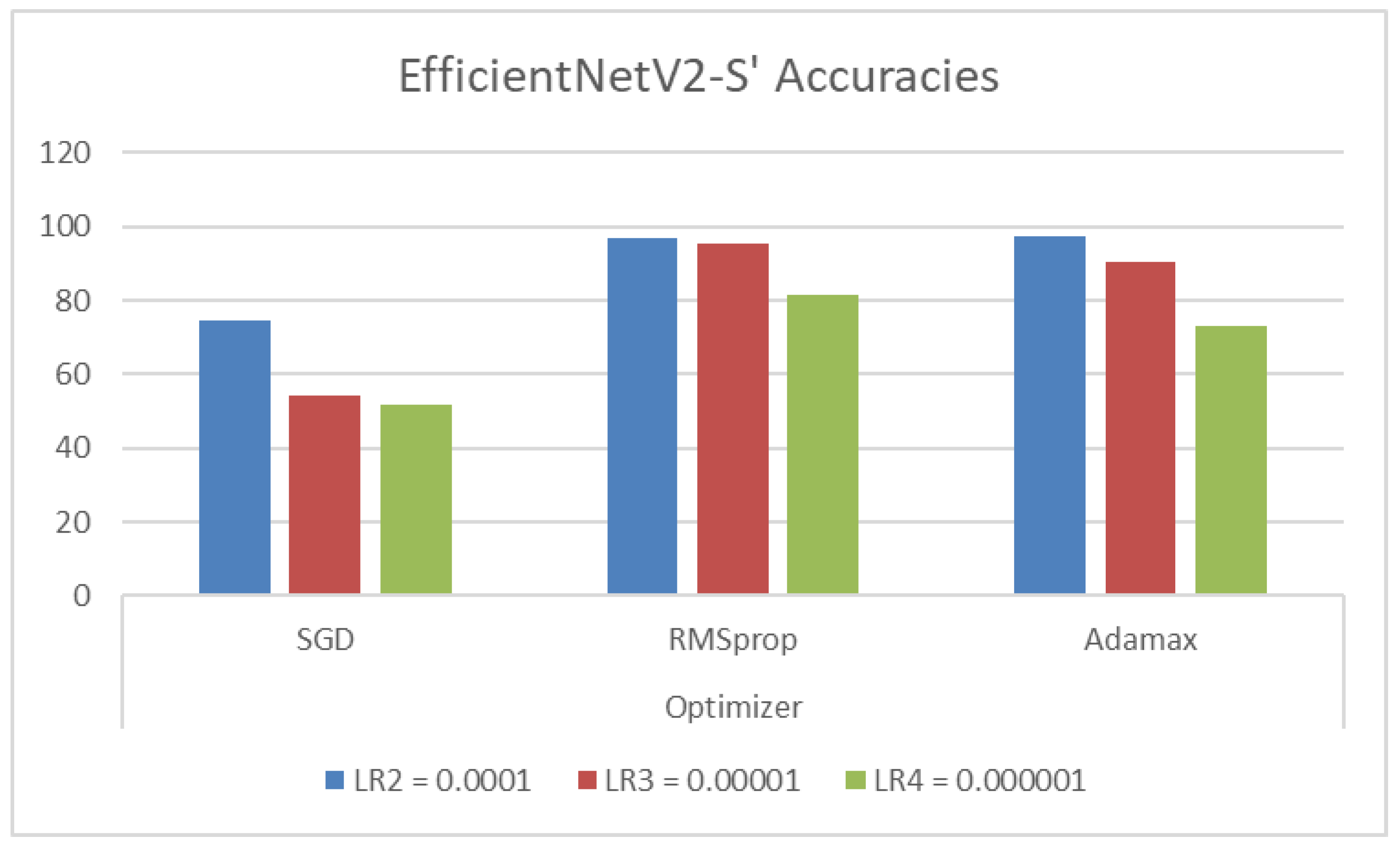
Patience	10

contains the hyperparameters utilized in our study and their respective values. The EfficientNetV2-S models utilized the Adamax optimizer during training with samples from the C-NMC_Leukemia dataset. During the training phase, modifications were applied to the initial weights of the models to enhance their effectiveness on this dataset. The training employed a constant learning rate set at 0.0001. While the training was limited to 30 epochs, an early stopping feature was integrated to observe the validation loss and terminate the training process as needed.

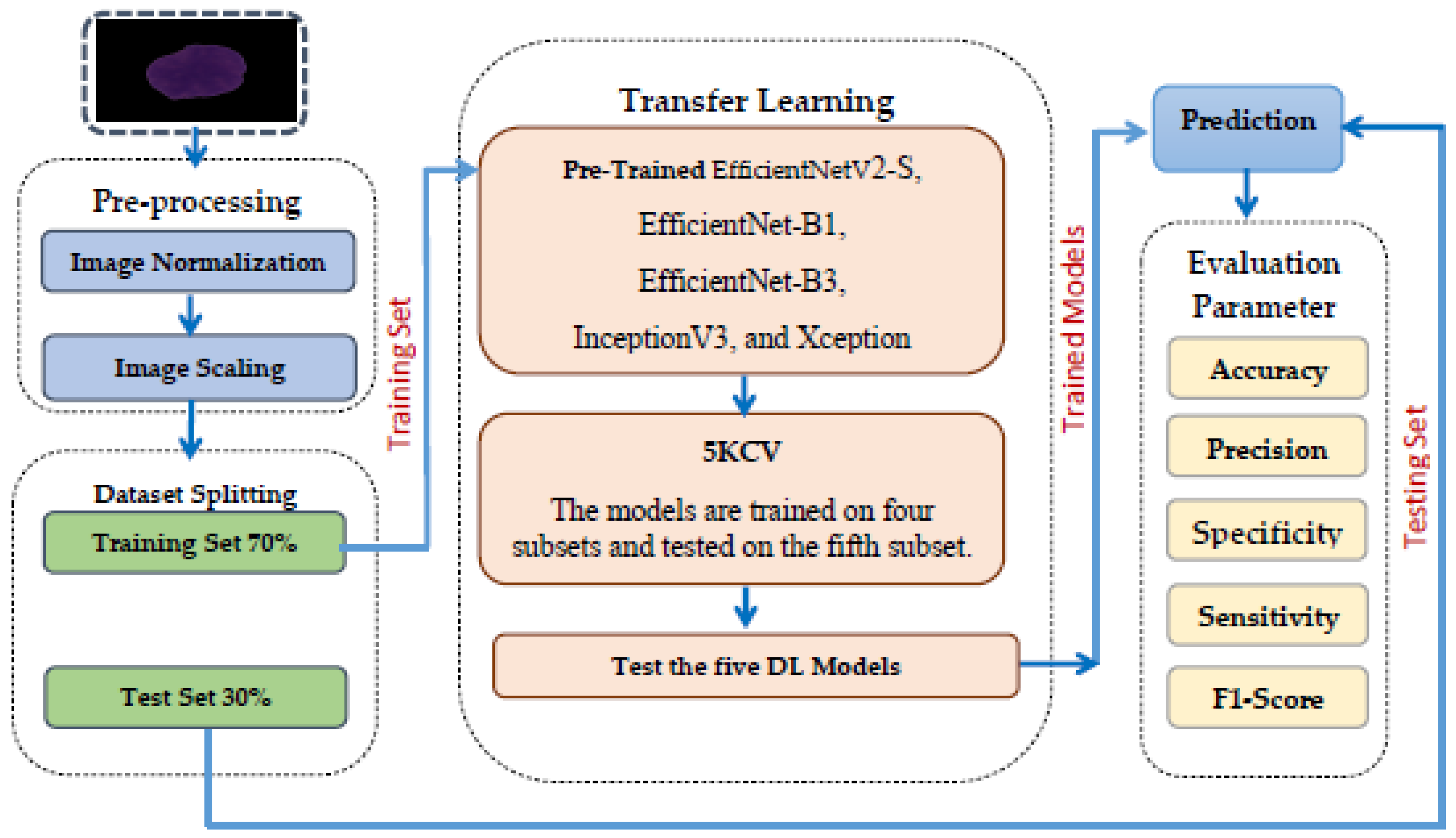
We divided the C-NMC_Leukemia dataset into two groups: a training set comprising 70% of all images (7264 images) and a testing set with the remaining 30% (3397 images). Finally, we evaluated the proposed model based on the criteria detailed in Equations (22)–(28).

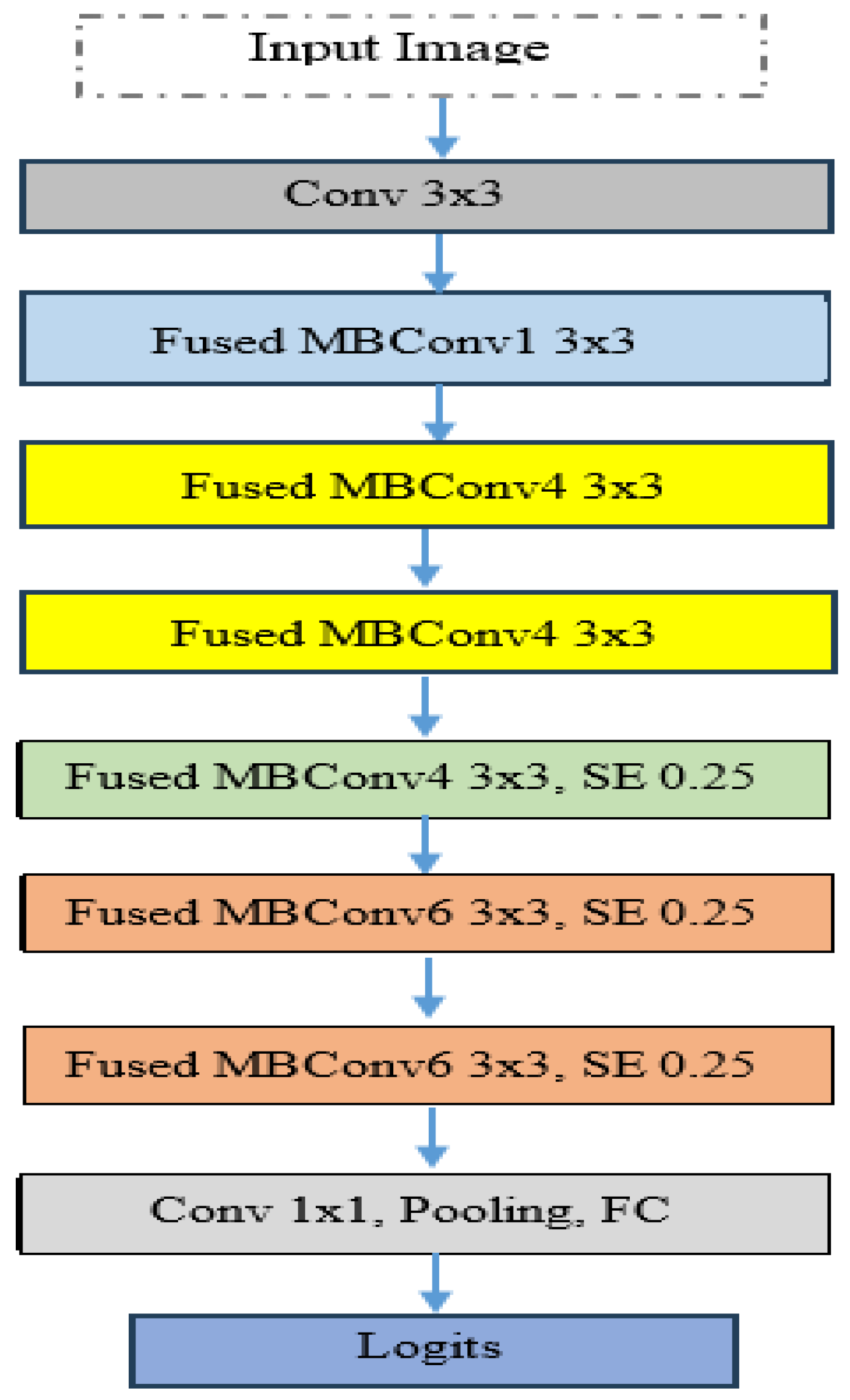
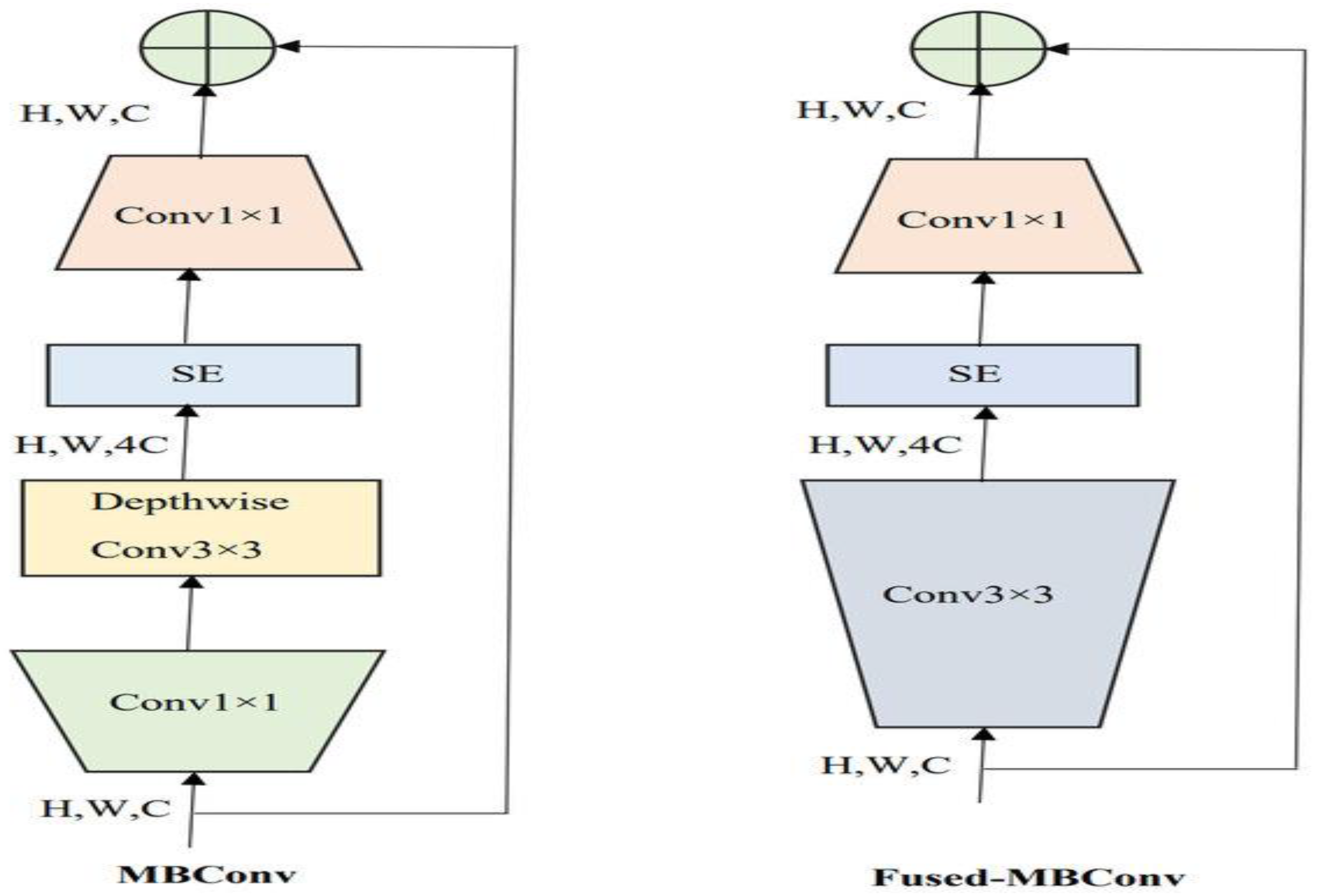
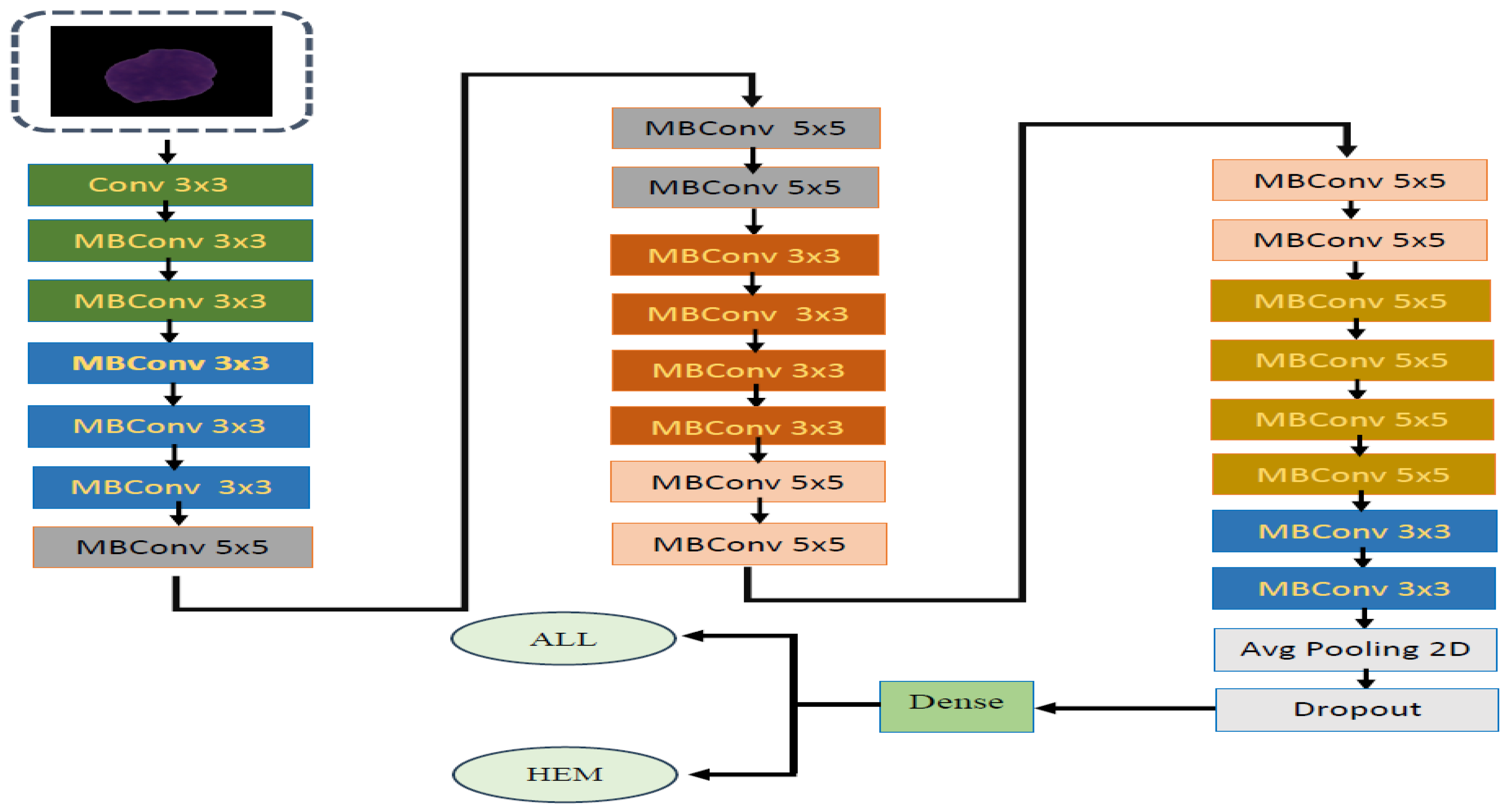
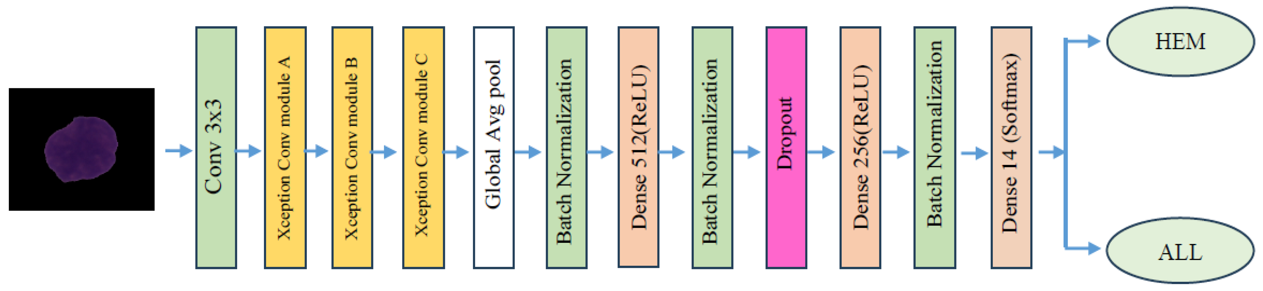
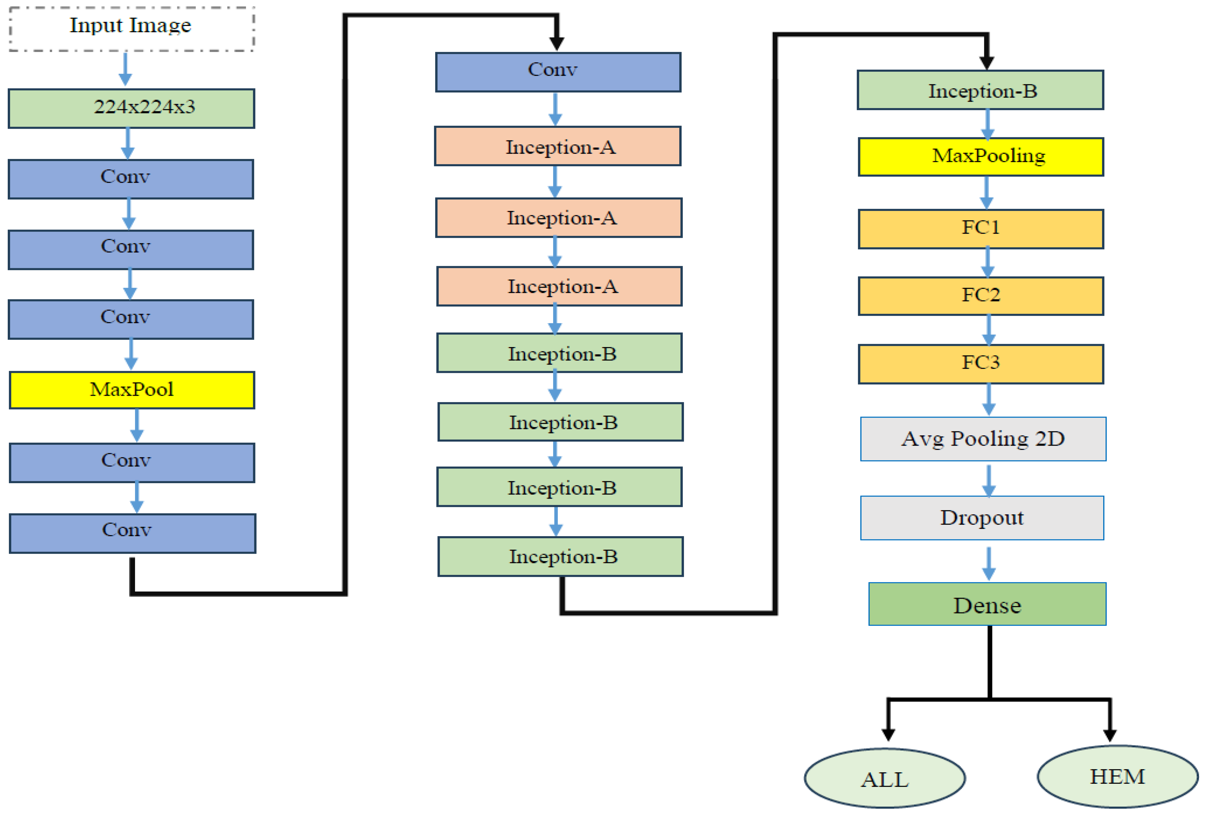
In the experiment, we identified ALL using the C-NMC_Leukemia dataset. Our approach involved developing a binary classification model utilizing the EfficientNetV2-S architecture to automate ALL detection. To improve the model’s efficiency, we integrated the 5KCV technique. Furthermore, we compared the performance of the EfficientNetV2-S model with four other DL models: EfficientNet-B1, EfficientNet-B3, InceptionV3, and Xception.

The main objective of this experiment was to identify ALL, aiming to enhance patient outcomes, streamline the diagnostic process, and significantly reduce patient time and expenses. The results from utilizing EfficientNetV2-S, EfficientNet-B1, EfficientNet-B3, InceptionV3, and Xception in conjunction with 5KCV are outlined in

Table 7. The 5KCV results of EfficientNetV2-S on the C-NMC_Leukemia’s test set.

EfficientNetV2-S	K-Folds	Accuracy (%)	Specificity (%)	Recall (%)	FNR (%)	Precision (%)	F1-Score (%)
	K1	97.822	97.822	97.822	2.178	97.822	97.822
	K2	97.321	97.321	97.321	2.679	97.321	97.321
	K3	97.351	97.351	97.351	2.649	97.351	97.351
	K4	96.880	96.880	96.880	3.120	96.883	96.880
	K5	97.321	97.321	97.321	2.679	97.333	97.321
	Avearge	97.339	97.339	97.339	2.661	97.342	97.339
	Confidence Interval	[97.07, 97.60]

,

Table 8. The 5KCV results of EfficientNet-B1 on the C-NMC_Leukemia’s test set.

EfficientNet-B1	Folds	Accuracy (%)	Specificity (%)	Recall (%)	FNR (%)	Precision (%)	F1-Score (%)
	K1	96.026	96.026	96.026	3.974	96.035	96.026
	K2	95.849	95.849	95.849	4.151	95.856	95.849
	K3	95.820	95.820	95.820	4.180	95.840	95.819
	K4	95.113	95.113	95.113	4.887	95.141	95.113
	K5	95.643	95.643	95.643	4.357	95.647	95.643
	Avearge	95.690	95.690	95.690	4.310	95.704	95.690
	Confidence Interval	[95.41, 95.96]

,

Table 9. The 5KCV results of EfficientNet-B3 on the C-NMC_Leukemia’s test set.

EfficientNet-B3	Folds	Accuracy (%)	Specificity (%)	Recall (%)	FNR (%)	Precision (%)	F1-Score (%)
	K1	95.849	95.850	95.850	4.150	95.887	95.848
	K2	96.526	96.526	96.526	3.474	96.526	96.526
	K3	96.497	96.497	96.497	3.503	96.504	96.497
	K4	96.173	96.173	96.173	3.827	96.175	96.173
	K5	96.320	96.320	96.320	3.680	96.321	96.320
	Avearge	96.273	96.273	96.273	3.727	96.283	96.273
	Confidence Interval	[96.056, 96.490]

,

Table 10. The 5KCV results of InceptionV3 on the C-NMC_Leukemia’s test set.

InceptionV3	Folds	Accuracy (%)	Specificity (%)	Recall (%)	FNR (%)	Precision (%)	F1-Score (%)
	K1	96.320	96.320	96.320	3.680	96.320	96.320
	K2	95.113	95.114	95.114	4.886	95.190	95.111
	K3	94.171	94.173	94.173	5.827	94.464	94.162
	K4	95.643	95.644	95.644	4.356	95.696	95.642
	K5	95.790	95.791	95.791	4.209	95.800	95.790
	Avearge	95.408	95.408	95.408	4.592	95.494	95.405
	Confidence Interval	[94.769, 96.045]

and

Table 11. The 5KCV results of Xception on the C-NMC_Leukemia test set.

Xception	Folds	Accuracy (%)	Specificity (%)	Recall (%)	FNR (%)	Precision (%)	F1-Score (%)
	K1	94.613	94.613	94.613	5.387	94.632	94.612
	K2	95.231	95.231	95.231	4.769	95.235	95.231
	K3	95.290	95.290	95.290	4.710	95.294	95.290
	K4	95.849	95.849	95.849	4.151	95.901	95.848
	K5	95.231	95.231	95.231	4.769	95.239	95.231
	Avearge	95.243	95.243	95.243	4.757	95.260	95.242
	Confidence Interval	[94.89, 95.58]

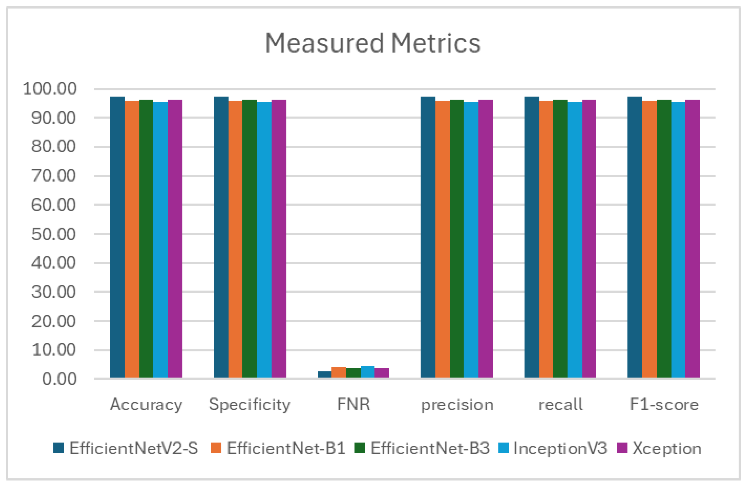
and Figure 8. These tables present the average assessment metrics for the proposed models used in the binary classification task on the C-NMC_Leukemia dataset’s test set. The average accuracies achieved were 97.339%, 95.690%, 96.273%, 95.408%, and 95.243%, respectively. As a result, the EfficientNetV2-S model demonstrated the highest level of accuracy.

EfficientNet-B1 achieved high performance with 97.339% specificity, recall, and precision. It showed a low FNR of 21.790% and maintained an impressive F1- score of 97.339%. EfficientNet-B3 demonstrated solid performance with 96.273% specificity, recall, and precision. It had a relatively low FNR of 3.727% and a commendable F1-score of 96.273%. InceptionV3 showed reliable performance with 95.408% specificity, recall, and precision. It had an FNR of 4.592% and an F1-score of 95.405%. Xception displayed consistent performance with 95.243% specificity, recall, and precision. It had an FNR of 4.757% and an F1-score of 95.242%.

The EfficientNetV2-S model has exhibited outstanding performance in various metrics such as accuracy, specificity, recall, NVP, precision, and F1-score. It attained the highest average values for accuracy, specificity, recall, and F1-score, reaching 97.339%. Moreover, it achieved the highest average values for precision, at 97.342%. Remarkably, it also showcased the lowest average FNR at 2.661%. These outcomes underscore the model’s excellence in binary classification tasks, demonstrating strong performance across various evaluation criteria.

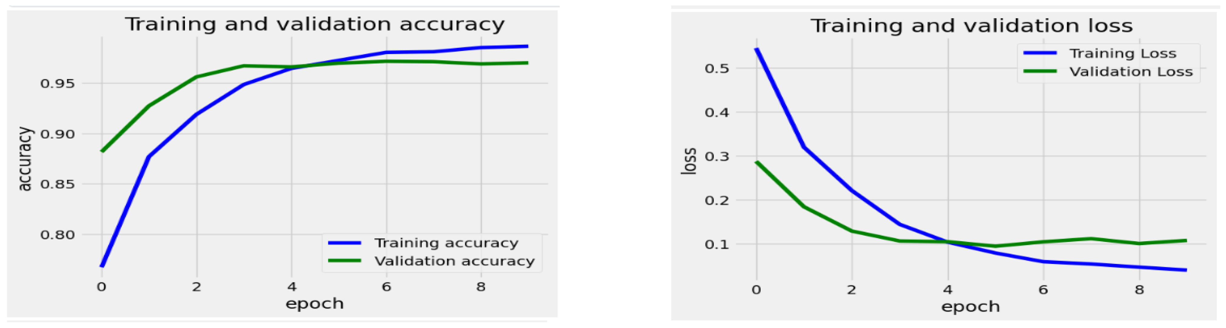
Figure 9, Figure 10, Figure 11, Figure 12 and Figure 13 display the progression of training and validation metrics across 8 epochs for the EfficientNetV2-S, the EfficientNet-B1, the EfficientNet-B3, the InceptionV3, and the Xception DL models. The graph on the right illustrates the loss values on the Y-axis against the number of epochs on the X-axis. A blue curve depicts the training loss and the validation loss by a green curve. On the left graph, accuracy is plotted on the Y-axis with epochs on the X-axis. The training accuracy is in blue, and the validation accuracy is in green. During the training of the EfficientNetV2-S model, the initial training loss was notably high at epoch 0, suggesting that the model had not yet undergone sufficient training. The loss consistently diminished as the training progressed through the subsequent epochs, indicating that the model was effectively improving and adapting to the training dataset. By epoch 9, the loss stabilized at a lower level, representing a point of diminishing returns for additional training. Similarly, the validation loss initially decreased, mirroring the trend observed in the training loss. This pattern suggests the model successfully generalized to new data during the earlier epochs.

The training accuracy began at a low point of approximately 78% during epoch 0. It showed a rapid increase in the early epochs, reaching about 95% accuracy by epoch 4. Following epoch 4, the training accuracy gradually rose, stabilizing just above 97% by epoch 9. In contrast, the validation accuracy started higher than the training accuracy at epoch 0, at around 89%. It also increased quickly in the initial epochs, nearing its peak of approximately 96% by epoch 4. However, after epoch 4, the validation accuracy plateaued, showing minimal improvement and maintaining stability while remaining below the training accuracy.

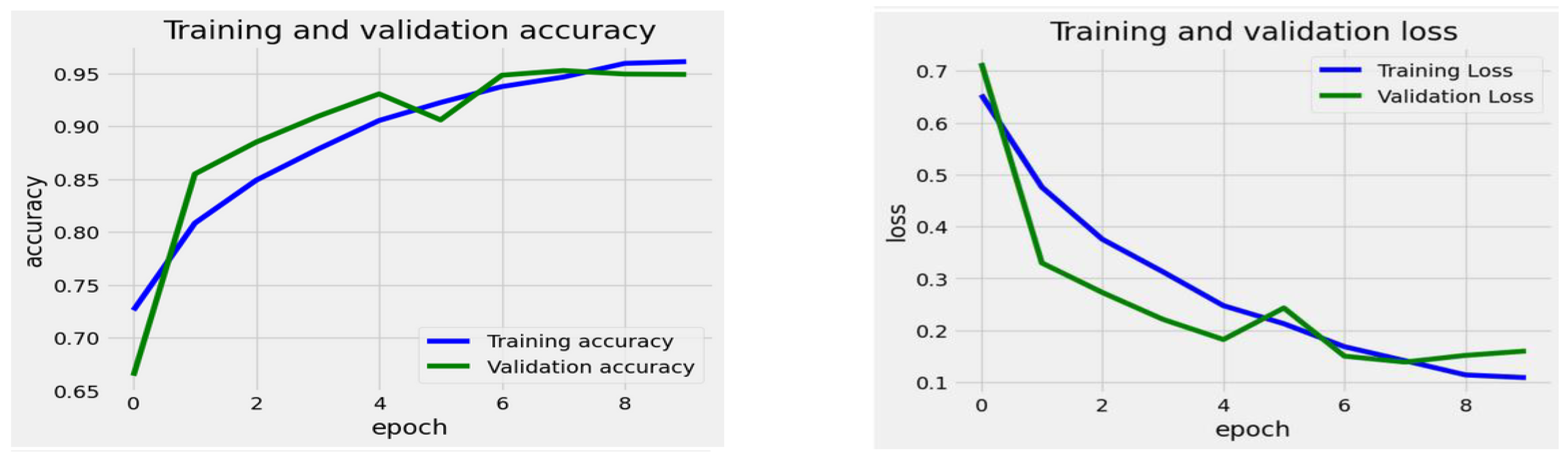
The training process for the EfficientNet-B1 Model began with a high training loss of about 0.7 during epoch 0. The loss consistently decreased as training progressed, indicating that the model improved its ability to learn from the training data. By epoch 9, the training loss had dropped to around 0.1, which reflects a successful error reduction on the training set. The validation loss followed a similar trend. It started at nearly 0.7 and experienced a significant decline in the initial epochs. However, there was a slight increase in the validation loss around epoch 6, suggesting some difficulties in generalization at that stage. After epoch 6, the validation loss resumed its downward trend, stabilizing at roughly 0.15 by epoch 9, which remained slightly higher than the training loss.

The training accuracy steadily improved over the epochs, starting at approximately 70% and stabilizing near 95% by the 9th epoch. In comparison, the validation accuracy initially increased rapidly, beginning at around 67%. It peaked around the 5th epoch, slightly surpassing the training accuracy, but then fluctuated slightly before stabilizing close to 95%. The overall results showed that the model attained high training and validation accuracy, indicating that the model learned effectively with minimal overfitting, as the two curves closely aligned after the initial epochs.

The EfficientNet-B3 Model began with an initial training loss of approximately 0.6. This loss steadily decreased throughout the training epochs, reaching about 0.1 by the 9th epoch. The validation loss followed a similar trend, although it experienced minor fluctuations. Notably, during the 5th and 6th epochs, the validation loss temporarily increased before continuing its downward trend. By the conclusion of the final epoch, the validation loss stabilized at around 0.1. The data indicates that the model’s loss consistently decreased for both the training and validation sets, highlighting effective learning. Although there were minor fluctuations in the validation loss, the overall downward trend suggests that the model did not experience significant overfitting.

The training accuracy increased steadily from approximately 75% at epoch 0 to nearly 96% by epoch 9, demonstrating continuous improvement. The validation accuracy initially rose sharply, starting at around 70%, and it soon surpassed the training accuracy. By the 5th epoch, it fluctuated slightly but remained closely aligned with the accuracy of the training. Eventually, it plateaued nearly 96% by the final epoch. The figure indicated that the training and validation accuracies closely matched, suggesting the model generalized well without significant overfitting. Both curves showed a consistent upward trend, stabilizing at a high accuracy level.

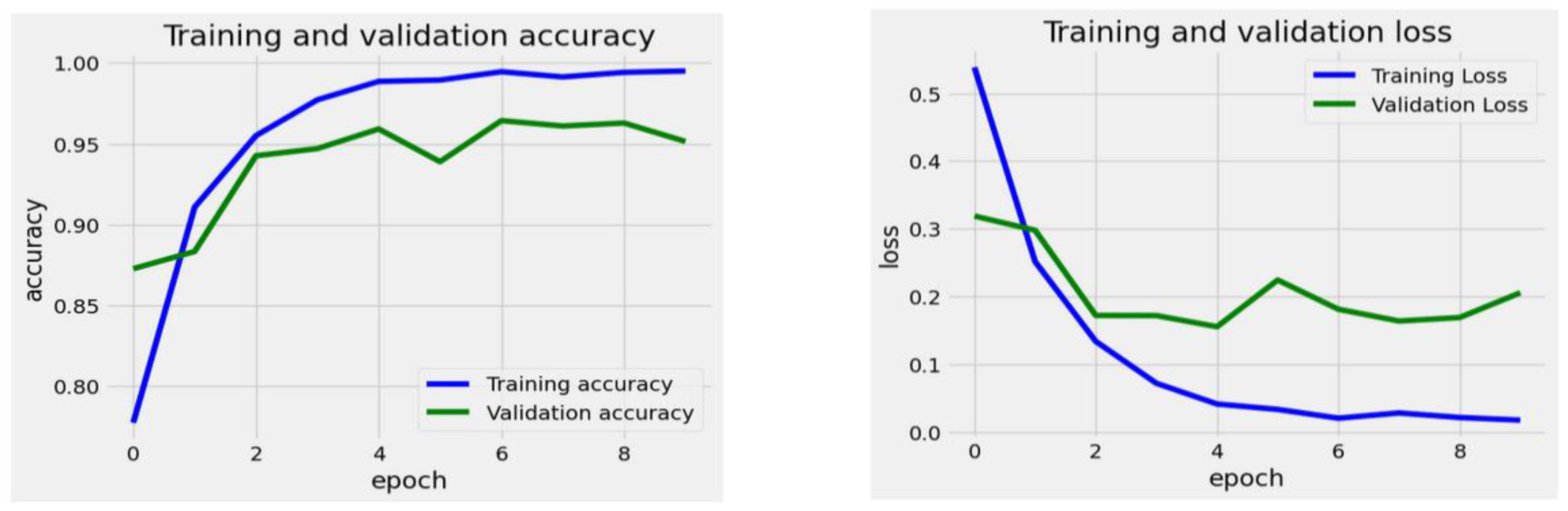
For the InceptionV3 model, the training loss started at around 0.55 during the first epoch and consistently decreased throughout the training process, reaching a low of approximately 0.02 by the ninth epoch. This trend indicates that the model successfully adapted to the training data over time. In contrast, the validation loss began at about 0.3 and dropped until around the second epoch. After this point, it stabilized and exhibited some variability. Notably, after the second epoch, the validation loss fluctuated between roughly 0.15 and 0.2, with a slight upward trend observed toward the end. The discrepancy between the training loss and validation loss suggests that the model may have overfitted to the training data. While the training loss continued to decline steadily, the validation loss did not show improvement after a few epochs, indicating that the model’s generalization ability did not enhance further.

The training accuracy began at approximately 0.8 during epoch 0 and steadily increased throughout the epochs, approaching 1.0 by epoch 9. This gradual rise indicates that the model effectively learned to make more accurate predictions on the training data. In contrast, the validation accuracy started at around 0.87 and experienced a rapid increase until epoch 2, reaching nearly 0.95. However, after epoch 2, it displayed minor fluctuations, remaining in the range of 0.95 to 0.97, without showing significant improvement. By epoch 9, it showed a slight decline compared to earlier values. The growing gap between training and validation accuracy over time suggests potential overfitting. While the model nearly memorized the training data perfectly, its performance on the validation set plateaued and did not improve, indicating that its ability to generalize to new, unseen data may be limited.

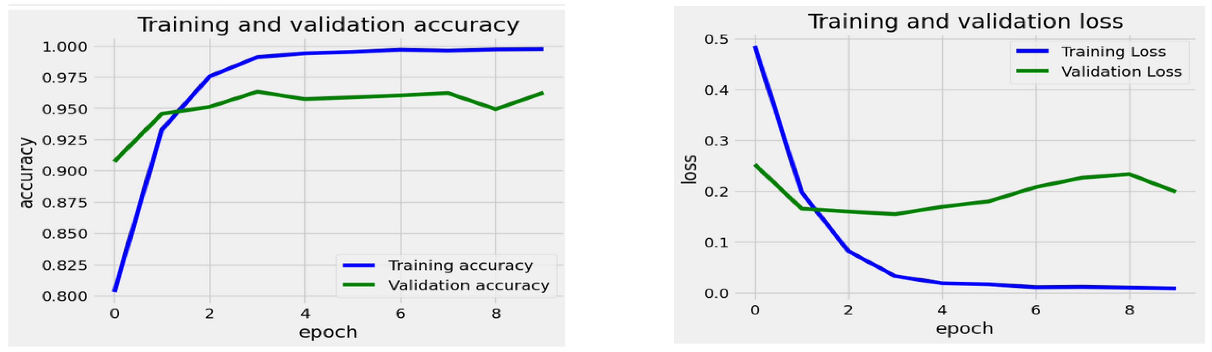
For the Xception model, the training loss started at around 0.5 during epoch 0 and showed a steady decline as the epochs progressed, eventually stabilizing near 0.02 by epoch 9. This consistent decrease indicates that the model effectively reduced losses on the training dataset over time. In contrast, the validation loss began at roughly 0.23 and initially decreased along with the training loss until it reached epoch 2. After epoch 2, the validation loss stabilized and began to show a slight increase, fluctuating between 0.17 and 0.23 in the subsequent epochs. The gap between training and validation loss after epoch 2 suggests that the model started to overfit the training data. While the training loss continued to decrease steadily, the validation loss stopped improving and began to rise, indicating a reduced ability to generalize to new, unseen data.

The training accuracy started at approximately 80% and increased rapidly during the first few epochs. By the end of the third epoch, it nearly reached 99% and remained consistent for the rest of the training, indicating that the model achieved almost perfect accuracy. The validation accuracy showed a similar upward trend but began to stabilize earlier. It peaked at around 95% after the third epoch and displayed minor fluctuations afterward, with slight decreases and recoveries, but it never surpassed the training accuracy. In conclusion, the data indicated that while the training accuracy reached 100%, the validation accuracy leveled off below this point, suggesting a potential overfitting of the training data. The gap between the curves highlighted the model’s limited capacity to generalize to new, unseen data.

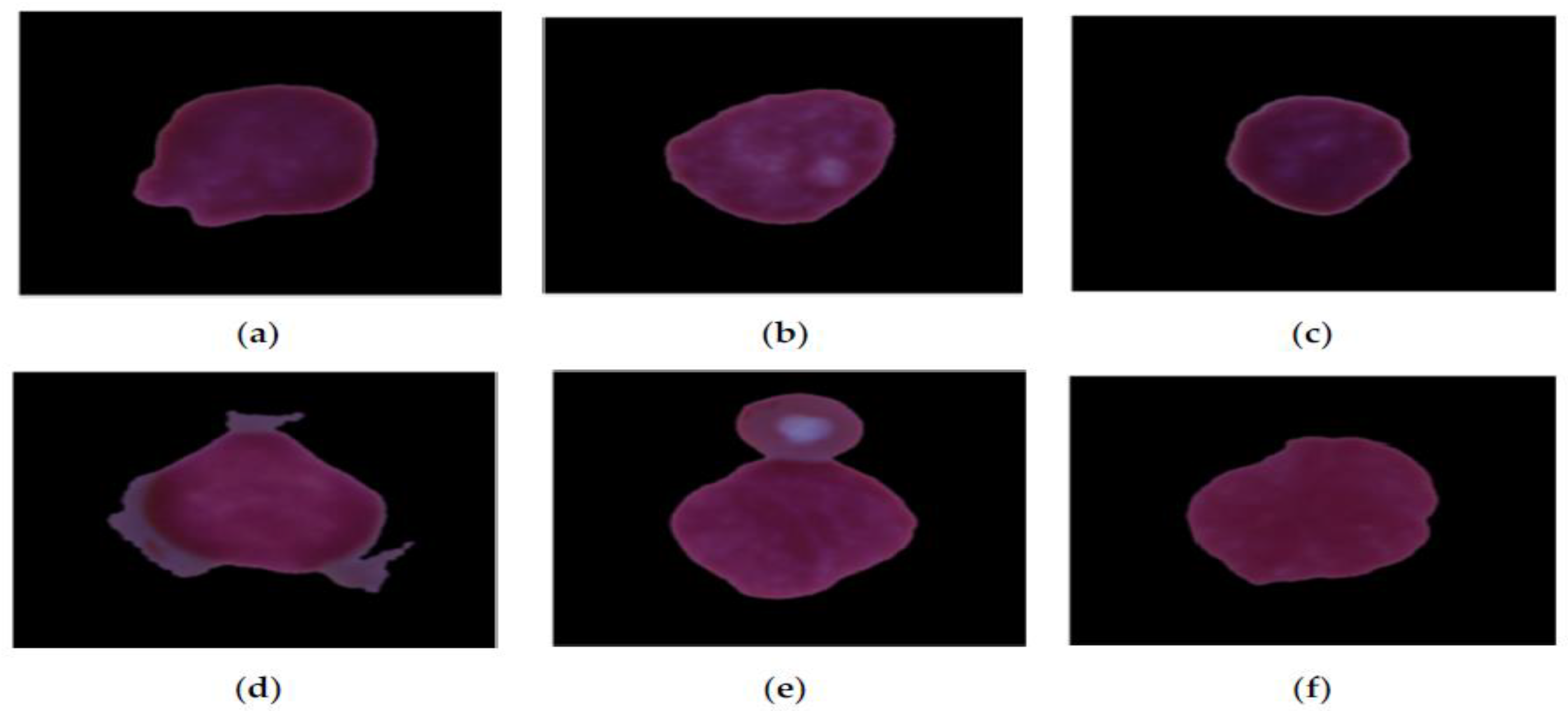
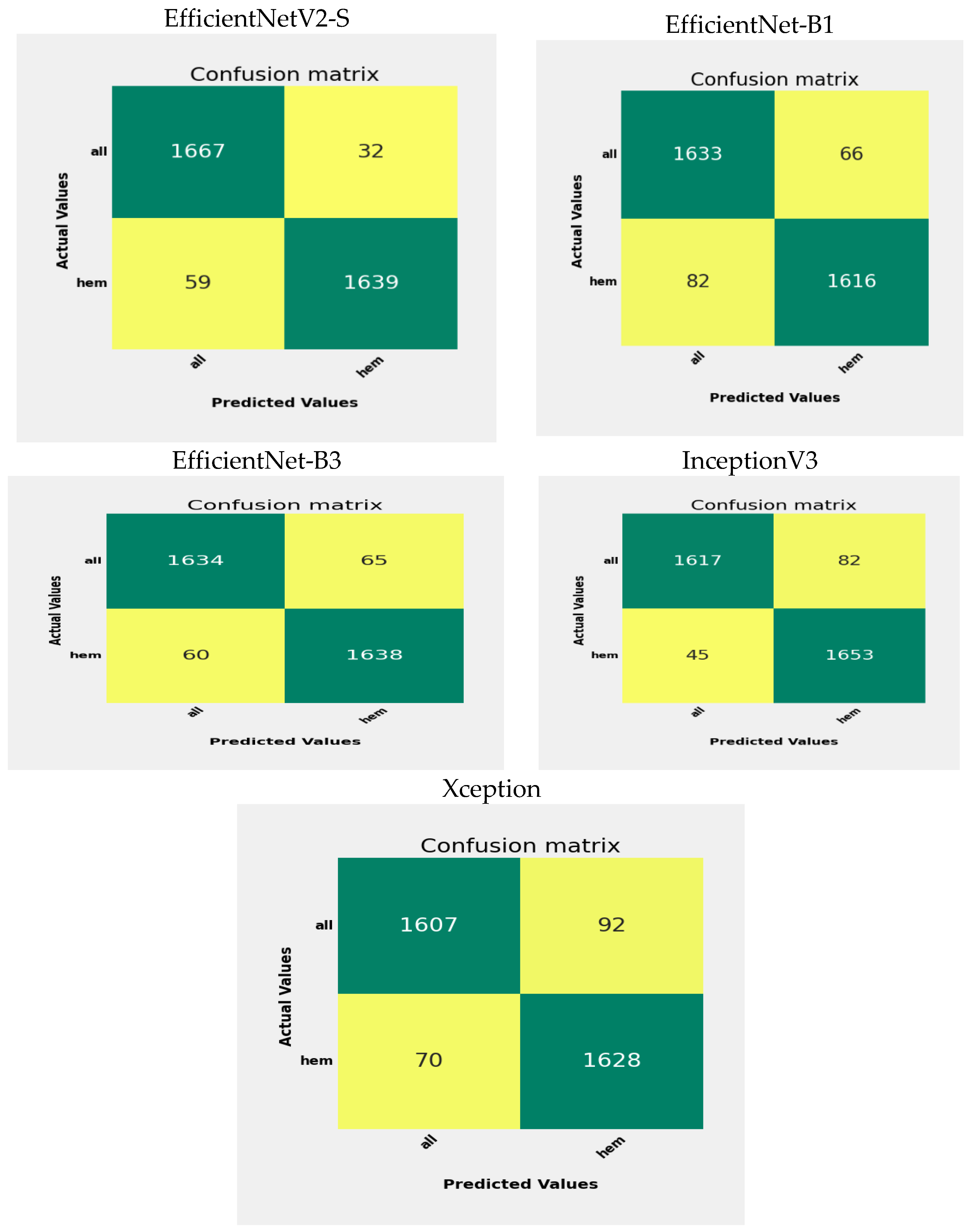
In Figure 14, we can observe the outcomes of testing the EfficientNetV2-S, EfficientNet-B1, EfficientNet-B3, InceptionV3, and Xception DL models on the C-NMC_Leukemia test set, which consists of two main categories: Healthy and ALL. The ALL category contains 1699 images, while the Healthy category comprises 1698 images.

Some specific counts indicate the performance of the EfficientNetV2-S model. The TP count is 1667, showing that the model accurately predicted 1667 instances belonging to the ALL class. The FP count is 32, meaning the model mistakenly identified 32 cases as ALL when they were Healthy, which suggests that the model has some difficulty distinguishing between the characteristics of ALL and Healthy in specific situations. Such misclassifications can occur because of similar visual features between ALL and Healthy and noise or artifacts in the images. The FN count is 59, indicating that the model incorrectly labeled 59 cases as Healthy when they were not. This type of misclassification stems from overlapping features or inadequate distinguishing patterns.

On the other hand, the TN count is 1639, demonstrating that the model correctly predicted 1639 instances that belonged to the Healthy class. Consequently, the precision for the ALL class stands at 98.1%, while the precision for the Healthy class is 96.5%. The model’s overall accuracy is approximately 97.3%, illustrating that the model accurately classified 97.3% of the instances.

In evaluating the EfficientNet-B1 model, the number of TP is 1633, indicating instances correctly predicted as ALL. Conversely, there are 66 FP instances incorrectly classified as ALL instead of Healthy. Moreover, 82 FN represent instances wrongly identified as Healthy instead of ALL. In contrast, there are 1616 TN, showing instances predicted correctly as Healthy by the model. The precision for the ALL class is 96.11%, denoting ALL predictions’ accuracy, while the Healthy class’s precision is 95.17%. The overall model accuracy is around 95.7%, meaning the model correctly classified 95.7% of instances.

When assessing the EfficientNet-B3 model, it correctly identified 1634 cases of ALL. However, it mistakenly classified 65 cases of Healthy as ALL. On the other hand, 60 cases of ALL were inaccurately labeled as Healthy. The model accurately recognized 1638 cases of health. The precision for the ALL category is 96.17%, signifying the correctness of its predictions for ALL. Similarly, the precision for the Healthy category is also 96.4%. The model’s overall accuracy is approximately 96.2%, accurately classifying 96.2% of cases.

When evaluating the InceptionV3 model, it correctly identified 1617 instances of ALL. However, it mistakenly categorized 82 Healthy cases as ALL. Conversely, it misclassified 45 ALL cases as Healthy. The model correctly detected 1653 Healthy cases. The precision for the ALL class is 95.17%, demonstrating the accuracy of its ALL predictions. Likewise, the precision for the Healthy class is 97.3%. The model’s overall accuracy is around 95.4%, showing that it correctly categorized 95.4% of instances.

When assessing the Xception model, it accurately recognized 1607 occurrences of ALL. Nonetheless, it erroneously labeled 92 Healthy instances as ALL. In contrast, it misidentified 70 ALL instances as Healthy. The model accurately identified 1628 Healthy occurrences. The precision for the ALL category stands at 94.6%, indicating the reliability of its ALL predictions. Similarly, the precision for the Healthy category is 95.8%. The model’s general accuracy hovers at approximately 95.2%, indicating that it precisely classified 95.2% of occurrences.

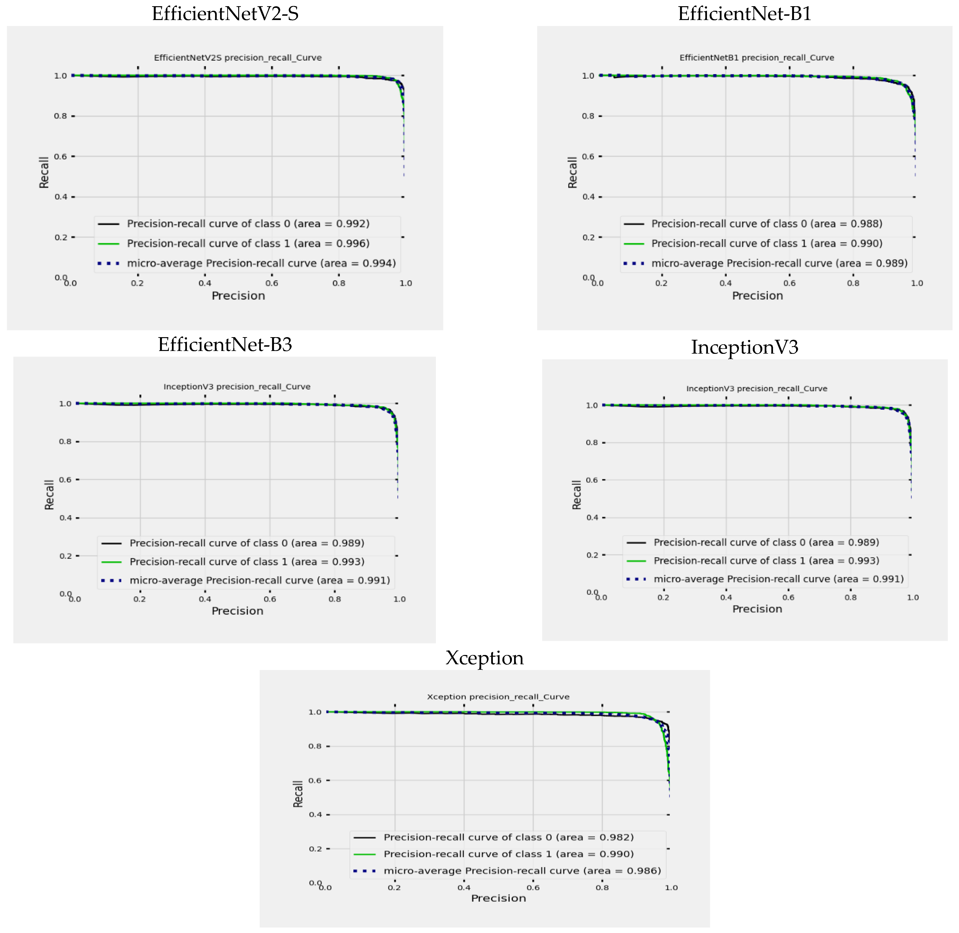
In Figure 15, you can see a graph illustrating the Precision-Recall (PR) curves for EfficientNetV2-S, EfficientNet-B1, EfficientNet-B3, InceptionV3, and Xception. This graph helps us understand how precision and recall values change based on different threshold settings. The X-axis (precision) represents the ratio of TP to the sum of TP and FP. It shows the accuracy of optimistic predictions made by the model. The Y-axis (recall) shows the ratio of TP to the sum of TP and FN. It reflects the model’s ability to identify all relevant cases within the dataset. The graph includes different lines:

• The black line depicts the precision-recall curve for class ALL.
• The green line illustrates the precision-recall curve for class Healthy.
• The blue dotted line represents the Micro-averaged precision-recall curve, which simultaneously considers precision and recall values across all classes.

For the EfficientNetV2-S model, the ALL class’s area under the curve (AUC) is 99.2%, indicating high precision and recall across various thresholds. Achieving a high AUC of 99.2% showcases exceptional performance predicting the ALL class. Similarly, the AUC for the Healthy class is 99.6%, signifying high precision and recall as well. With a remarkable AUC of 99.6%, the model demonstrates superior performance in predicting the Healthy class. Furthermore, the micro-averaged AUC of 99.4% presents an overall performance metric that combines the predictive capabilities comprehensively.

The performance of the EfficientNet-B1 model was evaluated using the area under the curve (AUC) metric. The AUC for the ALL class was found to be 98.8%, indicating strong precision and recall at different thresholds. This high AUC value of 98.8% demonstrates the model’s exceptional ability to predict the ALL class accurately. Similarly, the AUC for the Healthy class was 99.0%, showing excellent precision and recall. The model’s remarkable AUC score of 99.0% signifies its superior performance in predicting the Healthy class. Additionally, the micro-averaged AUC of 98.9% provides a comprehensive performance metric that reflects the overall predictive capabilities of the model.

For the EfficientNet-B3 model, the AUC for the ALL class is 98.9%, demonstrating excellent precision and recall across different thresholds. This high AUC of 98.9% indicates outstanding performance in predicting the ALL class. Similarly, the AUC for the Healthy class is 99.0%, highlighting strong precision and recall rates. The model achieves an impressive AUC of 99.0% in predicting the Healthy class. The micro-averaged AUC of 99.0% provides a comprehensive performance measure that effectively combines predictive capabilities.

The InceptionV3 model exhibits exceptional accuracy in classifying ALL and Healthy classes. The model demonstrates outstanding precision and recall at various thresholds, with an AUC of 98.9% for ALL and 99.3% for Healthy classes. These high AUC values signify the model’s exceptional predictive performance for both classes. Moreover, the micro-averaged AUC of 99.1% offers a holistic evaluation of the model’s overall predictive capabilities, showcasing its seamless effectiveness in combining predictive strengths.

The Xception model shows remarkable accuracy when distinguishing between the ALL and Healthy classes. It achieves an AUC of 98.2% for the ALL class and 99.0% for the Healthy class, highlighting its excellent precision and recall across different thresholds. The high AUC values indicate the model’s exceptional predictive ability for both classes. Additionally, the micro-averaged AUC of 98.6% provides a comprehensive assessment of the model’s overall predictive performance, demonstrating its seamless integration of predictive capabilities.

4.3. Ablation Study

An ablation study is a method used in ML and DL to evaluate how specific features or elements of a model affect its overall performance. In this process, certain parts of the model—like specific layers, modules, or parameters—are intentionally removed or changed one at a time to observe how these changes impact performance metrics. By comparing the results of the modified model with the original one, researchers can identify which components are crucial and which are less significant. This approach helps understand how the model operates, improve its design, and use resources better. Ablation studies are often employed to validate design choices, especially in complex systems like deep neural networks, and they clarify the contributions of different components to successful results.

In our Methodology, we performed an ablation analysis by adjusting the optimizers and learning rate (LR) settings. We began with the Adamax optimizer, using an LR of 0.0001, which produced an accuracy of 97.33%. Next, we experimented again with two additional optimizers: Stochastic Gradient Descent (SGD) and Root Mean Square Propagation (RMSprop). We tested LR values of 0.0001, 0.00001, and 0.000001 for each optimizer. The results, which show the accuracy of EfficientNetV2-S with different optimizers and LR values, are detailed in

Table 12. The EfficientNetV2-S’ accuracies with four optimizers and LR values.

EfficientNetV2-S	LR Value	Optimizer
		SGD	RMSprop	Adamax
	LR2 = 0.0001	74.8%	96.9%	97.33%
	LR3 = 0.00001	54.4%	95.6%	90.46%
	LR4 = 0.000001	51.7%	81.4%	73.2%

and illustrated in Figure 16.

According to the data in Table 12, when utilizing an LR2 = 0.0001, the Adamax optimizer achieved the highest accuracy of 97.33%. The RMSprop optimizer was closely followed with an accuracy of 96.9%. In contrast, the SGD optimizer demonstrated the least effectiveness at this learning rate, with a performance of only 74.8%. At a lower LR3 = 0.00001, the RMSprop optimizer yielded the best results, reaching an accuracy of 95.6%, while Adamax achieved a lower accuracy of 90.46%. Once again, the SGD optimizer trailed behind, achieving only 54.4% accuracy. For LR4 = 0.000001, all optimizers experienced a significant decline in performance. RMSprop achieved 81.4%, Adamax reached 73.2%, while SGD recorded the lowest performance with just 51.7%.

In summary, the Adamax optimizer consistently outperformed or matched the performance of other optimizers at higher learning rates, while RMSprop excelled at lower learning rates. Across all tested learning rates, the SGD optimizer was the least effective.

4.4. Discussion of the Outcomes of the Recent Literature

WBCs are essential components of the immune system. Unlike RBCs, which primarily transport oxygen, WBCs protect the body from infections and other foreign threats. These cells are generated in the bone marrow through a process called hematopoiesis. Within the bone marrow, HSCs differentiate into various types of blood cells, including WBCs. Once they reach full maturity, WBCs enter the bloodstream and surrounding tissues to perform their immune functions. Anomalies in the quantity, size, structure, or function of WBCs can disrupt the bone marrow’s ability to produce vital blood components, potentially weakening the immune system. Abnormal WBCs can crowd out normal blood cells, leading to decreased RBCs, WBCs, and platelets. Additionally, suppose cancerous WBCs circulate in the bloodstream. In that case, they may harm essential organs such as the liver, kidneys, spleen, and brain, which result in severe complications, including infections, disorders of the immune system, and blood-related cancers, such as leukemia.

This research aims to create a strong and optimized model based on the EfficientNetV2-S architecture to classify ALL diseases into two categories: ALL and Healthy. The study used the 5KCV technique, which allowed for effective fine-tuning of the model’s parameters to improve the performance of the EfficientNetV2-S model. By using 5KCV, we achieved a more thorough evaluation of the model’s performance compared to a single train-test split. The use of multiple folds helps to minimize variability in performance estimates. The average performance across the five folds is typically more stable and reliable than that from just one train-test split. Cross-validation is useful for identifying overfitting, where a model performs well on training data but poorly on validation data. This feedback is crucial for adjusting the model and selecting the right features. Cross-validation is also commonly used in hyperparameter tuning to determine the best model parameters, providing a reliable performance estimate for each parameter set and assisting in selecting the optimal choice. As a result, this fine-tuned model achieved superior outcomes compared to recent techniques outlined in

Table 13. Comparison of the proposed model’s results with recent models’ results.

Reference	Methodology	Accuracy	Datasets
Mondal et al. [24]	CNN	88.3%	C-NMC_Leukemia
R. Khandekar et al. [25]	YOLO	mAP: 98.7%.	C-NMC_Leukemia
Almadhor et al. [26]	NB, KNN, RF, and SVM	SVM: 90%	C-NMC_Leukemia
Kasani et al. [27]	DL	96.58%	C-NMC_Leukemia
Liu et al. [28]	a ternary stream-driven weakly supervised data augmentation classification network (WT-DFN)	91.90%	C-NMC_Leukemia
Sulaiman et al. [29]	ResRandSVM	90%	C-NMC_Leukemia
Proposed model	5KCV and EfficientNetV2-S	97.33%	C-NMC_Leukemia

.

In Table 13, various ML and DL techniques were utilized. These included CNNs as presented by Mondal et al. [20], YOLO by R. Khandekar et al. [21], and traditional ML models such as NB, KNN, RF, and SVM used by Almadhor et al. [22]. Additionally, advanced DL models featuring specialized architectures were employed in the studies by Kasani et al. [23] and Liu et al. [24]. Hybrid models, such as those by Sulaiman et al. [25], were also explored, and they combined ResNet features with RF and SVM.

Our proposed model, which integrated EfficientNetV2-S with a 5KCV approach, achieved the highest classification accuracy of 97.33%, surpassing all other models. This result underscores the effectiveness of EfficientNetV2-S alongside 5KCV. The YOLO model (Khandekar et al. [21]) attained a mAP of 98.7%. The second-highest classification accuracy was recorded by Kasani et al. [23], with a score of 96.58% using DL techniques. Traditional ML methods, as demonstrated by Almadhor et al. [22], showed comparatively lower performance, with SVM achieving the best result among them at 90%.

EfficientNetV2-S is recognized as a state-of-the-art DL model and is noted for its efficiency and scalability, factors that likely contribute to its high accuracy. Implementing 5KCV enhanced the robustness of the findings by minimizing overfitting and providing a dependable estimate of the model’s generalization capabilities.

In summary, the proposed model demonstrated the best classification accuracy (97.33%) on the C-NMC_Leukemia dataset, showcasing the promise of EfficientNetV2-S when combined with rigorous evaluation methods such as 5KCV.

5. Conclusions

This research developed a robust and optimized model based on the EfficientNetV2-S architecture to classify Acute Lymphoblastic Leukemia (ALL) into ALL and Healthy categories. The study employed the 5KCV technique, which allowed for effective fine-tuning of the model’s parameters to enhance the efficiency of the EfficientNetV2-S model. This proposed model is vital for helping hematologists identify ALL early, resulting in improved patient outcomes and a quicker, more cost-effective diagnostic process. This approach aims to decrease both the time required and the patient costs. An experiment was conducted using the C-NMC_Leukemia dataset, specifically for diagnosing ALL. To ensure consistent data input, the dataset underwent initial processing steps, including resizing and standardization. It was divided into 70% for training and validation and 30% for testing. Comparative analyses with other models, such as EfficientNet-B1, EfficientNet-B3, InceptionV3, and Xception, showed that the EfficientNetV2-S model achieved outstanding performance metrics, with an average recall, accuracy, specificity, and F1-score of 97.34%, alongside a precision of 97.34%. The evaluation highlighted that the proposed model, with appropriate adjustments, outperformed existing models, demonstrating its effectiveness in detecting ALL. Compared to traditional classification systems, the remarkable performance of our proposed model was clear. Our classifier’s assessment underscored our Methodology’s potential, proving its effectiveness in accurately identifying ALL. The speed of processing poses a challenge for our proposed model. In our future research, we will explore the proposed model across various human cancer types and employ hyper-optimization algorithms to automate the improvement of hyper-parameters. We will also integrate confidence levels as a measurement metric. Additionally, we plan to implement the reinforced transformer network (RTN), which combines the benefits of reinforcement learning and transformer models to assess image quality. This method may be particularly useful in identifying and improving the diagnostic quality of ALL scans, which are crucial for detecting ALL diseases.

References

1. Ansari, S.; Navin, A.A.H.; Sangar, A.B.; Gharamaleki, J.V.; Danishvar, S.A. Customized Efficient Deep Learning Model for the Diagnosis of Acute Leukemia Cells Based on Lymphocyte and Monocyte Images. Electronics 2023, 12, 322. [Google Scholar] [CrossRef]
2. Deshpande, N.M.; Gite, S.; Aluvalu, R. A review of microscopic analysis of blood cells for disease detection with AI perspective. PeerJ Comput. Sci. 2021, 7, e460. [Google Scholar] [CrossRef] [PubMed]
3. Chen, T.C.; Minea, R.O.; Swenson, S.; Yang, Z.; Thein, T.Z.; Schönthal, A.H. NEO212, a perillyl alcohol-temozolomide conjugate, triggers macrophage differentiation of acute myeloid leukemia cells and blocks their tumorigenicity. Cancers 2022, 14, 6065. [Google Scholar] [CrossRef] [PubMed]
4. Alsalem, M.A.; Zaidan, A.A.; Zaidan, B.B.; Hashim, M.; Madhloom, H.T.; Azeez, N.D.; Alsyisuf, S. A review of the automated detection and classification of acute leukaemia: Coherent taxonomy, datasets, validation and performance measurements, motivation, open challenges and recommendations. Comput. Methods Programs Biomed. 2018, 158, 93–112. [Google Scholar] [CrossRef]
5. Oskouei, V.G.; Saatlo, A.N.; Sheykhivand, S.; Farzamnia, A. An Experimental Study: ICA-Based Sensorimotor Rhythms Detection in ALS Patients for BCI Applications. In Proceedings of the International Conference on Computer, Information Technology and Intelligent Computing (CITIC 2022), Kuala Lumpur, Malaysia, 25–27 July 2022; pp. 145–155. [Google Scholar]
6. Aftab, M.O.; Awan, M.J.; Khalid, S.; Javed, R.; Shabir, H. Executing spark BigDL for leukemia detection from microscopic images using transfer learning. In Proceedings of the 1st International Conference on Artificial Intelligence and Data Analytics (CAIDA), Riyadh, Saudi Arabia, 6–7 April 2021; pp. 216–220. [Google Scholar]
7. Anilkumar, K.K.; Manoj, V.J.; Sagi, T.M. Automated detection of B cell and T cell acute lymphoblastic leukaemia using deep learning. IRBM 2021, 43, 405–413. [Google Scholar] [CrossRef]
8. Terwilliger, T.; Abdul-Hay, M. Acute lymphoblastic leukemia: A comprehensive review and 2017 update. Blood Cancer J. 2017, 7, e577. [Google Scholar] [CrossRef] [PubMed]
9. Lashway, S.G.; Harris, R.B.; Farland, L.V.; O’Rourke, M.K.; Dennis, L.K. Age and cohort trends of malignant melanoma in the United States. Cancers 2021, 13, 3866. [Google Scholar] [CrossRef]
10. Mustaqim, T.; Fatichah, C.; Suciati, N. Deep Learning for the Detection of Acute Lymphoblastic Leukemia Subtypes on Microscopic Images: A Systematic Literature Review. IEEE Access 2023, 11, 16108–16127. [Google Scholar] [CrossRef]
11. Ouyang, N.; Wang, W.; Ma, L.; Wang, Y.; Chen, Q.; Yang, S.; Xie, J.; Su, S.; Cheng, Y.; Cheng, Q.; et al. Diagnosing acute promyelocytic leukemia by using convolutional neural network. Clin. Chim. Acta 2021, 512, 1–6. [Google Scholar] [CrossRef] [PubMed]
12. Pałczyński, K.; Śmigiel, S.; Gackowska, M.; Ledziński, D.; Bujnowski, S.; Lutowski, Z. IoT application of transfer learning in hybrid artificial intelligence systems for acute lymphoblastic leukemia classification. Sensors 2021, 21, 8025. [Google Scholar] [CrossRef]
13. Hallböök, H.; Gustafsson, G.; Smedmyr, B.; Söderhäll, S.; Heyman, M. Treatment outcome in young adults and children >10 years of age with acute lymphoblastic leukemia in sweden: A comparison between a pediatric protocol and an adult protocol. Cancer 2006, 107, 1551–1561. [Google Scholar] [CrossRef]
14. Chen, Y.; Wu, C.; Zhang, Z.; Goldstein, J.A.; Gernand, A.D.; Wang, J.Z. PlacentaNet: Automatic morphological characterization of placenta photos with deep learning. In Proceedings of the 22nd International Conference, Shenzhen, China, 13–17 October 2019; pp. 487–495. [Google Scholar]
15. Hagos, Y.B.; Narayanan, P.L.; Akarca, A.U.; Marafioti, T.; Yuan, Y. ConCORDe-Net: Cell count regularized convolutional neural network for cell detection in multiplex immunohistochemistry images. In Proceedings of the 22nd International Conference, Shenzhen, China, 13–17 October 2019; pp. 667–675. [Google Scholar]
16. Wang, X.; Xu, M.; Li, L.; Wang, Z.; Guan, Z. Pathology-aware deep network visualization and its application in glaucoma image synthesis. In Proceedings of the 22nd International Conference, Shenzhen, China, 13–17 October 2019; pp. 423–431. [Google Scholar]
17. Burke, J.S. The value of the bone-marrow biopsy in the diagnosis of hairy cell leukemia. Am. J. Clin. Pathol. 1978, 70, 876–884. [Google Scholar] [CrossRef] [PubMed]
18. Klingebiel, T.; Cornish, J.; Labopin, M.; Locatelli, F.; Darbyshire, P.; Handgretinger, R.; Balduzzi, A.; Owoc-Lempach, J.; Fagioli, F.; Or, R.; et al. Results and factors influencing outcome after fully haploidentical hematopoietic stem cell transplantation in children with very high-risk acute lymphoblastic leukemia: Impact of center size: An analysis on behalf of the acute leukemia and pediatric disease working parties of the european blood and marrow transplant group. Blood 2010, 115, 3437–3446. [Google Scholar] [PubMed]
19. Ahmed, I.A.; Senan, E.M.; Shatnawi, H.S.A.; Alkhraisha, Z.M.; Al-Azzam, M.M.A. Hybrid techniques for the diagnosis of acute lymphoblastic leukemia based on fusion of CNN features. Diagnostics 2023, 13, 1026. [Google Scholar] [CrossRef] [PubMed]
20. Mondal, C.; Hasan, K.; Ahmad, M.; Awal, A.; Jawad, T.; Dutta, A.; Islam, R.; Moni, M.A. Ensemble of convolutional neural networks to diagnose acute lymphoblastic leukemia from microscopic images. Inform. Med. Unlocked 2021, 27, 100794. [Google Scholar] [CrossRef]
21. Khandekar, R.; Shastry, P.; Jaishankar, S.; Faust, O.; Sampathila, N. Automated blast cell detection for acute lymphoblastic leukemia diagnosis. Biomed. Signal Process. Control 2021, 68, 102690. [Google Scholar] [CrossRef]
22. Almadhor, A.; Sattar, U.; Al Hejaili, A.; Mohammad, U.G.; Tariq, U. An efficient computer vision-based approach for acute lymphoblastic leukemia prediction. Front. Comput. Neurosci. 2022, 16, 1083649. [Google Scholar] [CrossRef]
23. Kasani, P.H.; Won Park, S.; Won Jang, J. An aggregated-based deep learning method for leukemic b-lymphoblast classification. Diagnostics 2020, 10, 1064. [Google Scholar] [CrossRef]
24. Liu, Y.; Chen, P.; Zhang, J.; Liu, N.; Liu, Y. Weakly supervised ternary stream data augmentation fine-grained classification network for identifying acute lymphoblastic leukemia. Diagnostics 2022, 12, 16. [Google Scholar] [CrossRef]
25. Sulaiman, A.; Kaur, S.; Gupta, S.; Alshahrani, H.; Al Reshan, M.S.; Alyami, S.; Shaikh, A. ResRandSVM: Hybrid approach for acute lymphocytic leukemia classification in blood smear images. Diagnostics 2023, 13, 2121. [Google Scholar] [CrossRef] [PubMed]
26. Kaggle. Leukemia Dataset. Available online: https://www.kaggle.com/datasets/avk256/cnmc-leukemia (accessed on 10 October 2022).
27. Tan, M.; Le, Q.V. EfficientNetV2: Smaller models and faster training. arXiv 2021, arXiv:2104.00298. [Google Scholar]
28. Alhichri, H.; Alswayed, A.S.; Bazi, Y.; Ammour, N.; Alajlan, N.A. Classification of remote sensing images using EfficientNet-B3 CNN model with attention. IEEE Access 2021, 9, 14078–14094. [Google Scholar] [CrossRef]
29. Ahmed, T.; Sabab, N.H.N. Classification and understanding of cloud structures via satellite images with EfficientUNet. arXiv 2021, arXiv:2009.12931. [Google Scholar] [CrossRef]
30. He, K.; Zhang, X.; Ren, S.; Sun, J. Deep Residual Learning for Image Recognition. arXiv 2015, arXiv:1512.03385. [Google Scholar]
31. Francois, C. Deep learning with depthwise separable convolutions. arXiv 2016, arXiv:1610.02357. [Google Scholar]
32. Szegedy, C.; Vanhoucke, V.; Ioffe, S.; Shlens, J.; Wojna, Z. Rethinking the inception architecture for computer vision. In Proceedings of the IEEE Conference on Computer Vision and Pattern Recognition (CVPR), Las Vegas, NV, USA, 27–30 June 2016; pp. 2818–2826. [Google Scholar]
Figure 1. Images (ac) show healthy individuals, and images (df) display cases of ALL [25].
Symmetry 17 00024 g001
Figure 2. The proposed model architecture.
Symmetry 17 00024 g002
Figure 3. The proposed EfficientNetV2-S model architecture.
Symmetry 17 00024 g003
Figure 4. Structure of MBConv and Fused-MBConv.
Symmetry 17 00024 g004
Figure 5. The architecture of EfficientNet-B1.
Symmetry 17 00024 g005
Figure 6. The architecture of Xception.
Symmetry 17 00024 g006
Figure 7. The InceptionV3 model’s architecture.
Symmetry 17 00024 g007
Figure 8. The measured metrics of the five DL models.
Symmetry 17 00024 g008
Figure 9. The accuracy VS. loss of EfficientNetV2-S.
Symmetry 17 00024 g009
Figure 10. The accuracy VS. loss of EfficientNet-B1.
Symmetry 17 00024 g010
Figure 11. The accuracy VS. loss of EfficientNet-B3.
Symmetry 17 00024 g011
Figure 12. The accuracy VS. loss of InceptionV3.
Symmetry 17 00024 g012
Figure 13. The accuracy VS. loss of Xception.
Symmetry 17 00024 g013
Figure 14. The confusion matrices over the C-NMC_Leukemia’s test set for the five DL models.
Symmetry 17 00024 g014
Figure 15. The PR curves over the C-NMC_Leukemia’s test set for the five DL models.
Symmetry 17 00024 g015
Figure 16. The EfficientNetV2-S’ accuracies with three optimizers and three LR values.
Symmetry 17 00024 g016