A Symmetry-Inspired Hierarchical Control Strategy for Preventing Rollover in Articulated Rollers

Abstract

In off-road environments, the lateral rollover stability of articulated unmanned rollers (URs) is critical to ensure operational safety and efficiency. This paper introduces the concept of a rollover energy barrier (REB), a symmetry-based metric that quantifies the energy margin between the current state and the critical rollover threshold of articulated rollers. URs exhibit dynamic asymmetry due to their hydraulic steering systems, which differ significantly from traditional passenger vehicles. To address these challenges, we propose a hierarchical control framework inspired by the principles of dynamic symmetry. This framework integrates Nonlinear Model Predictive Control (NMPC) and Active Disturbance Rejection Control (ADRC): NMPC is used for trajectory planning by incorporating the REB into the cost function, ensuring rollover stability, while ADRC compensates for dynamic asymmetries, model uncertainties, and external disturbances during trajectory tracking. Simulation and experimental results validate the effectiveness of the proposed control strategy in enhancing the rollover stability and tracking performance of the URs under off-road conditions.

1. Introduction

Single-drum articulated rollers are widely used in construction and road maintenance for soil compaction tasks [1]. Advancements in control technology have made URs increasingly indispensable [2,3]. The URs not only enhance operational safety and reduce labor costs but also allow for precise control and data monitoring.

In practical applications, the special working environment and vehicle structure of URs as illustrated in Figure 1 make trajectory tracking control difficult. The URs typically operate in off-road environments with bumps and depressions [4], posing significant challenges to rollover stability [5]. These challenges arise from the dynamic asymmetry caused by uneven terrain and the articulated structure, disrupting the energy balance and stability. In addition, the dynamics of articulated vehicles are inherently nonlinear and involve strong coupling between mechanical and hydraulic components [6]. The hydraulic steering system, in particular, exhibits complex behaviors, introducing functional asymmetry between the vehicle’s front and rear bodies, which imposes a substantial computational burden on the MPC solver [7]. There are also some unmodeled disturbances from the environment and vehicles that affect the control performance. This complexity necessitates advanced control strategies capable of handling nonlinearities and uncertainties to ensure rollover stability.

The cause of rollover can be attributed to road factors and operational factors, such as uneven road surfaces and aggressive driving by drivers. Based on these factors, the rollovers are categorized into two types: tripped rollovers and untripped rollovers [8,9]. An untripped rollover occurs due to aggressive maneuvering on flat ground, while a tripped rollover is often caused by unbalanced roll torque generated by uneven terrains, such as one wheel hitting a protruding rock. This study focuses primarily on tripped rollovers, with untripped rollovers receiving only brief consideration. To ensure rollover stability in trajectory tracking control, the control strategy has evolved into two key components: rollover stability assessment and trajectory tracking control [10].

To access the rollover risk, some indices have been developed. Initially, the Static Stability Index (SSI) was adopted [11,12,13,14], often defined as the threshold values of specific state variables, such as roll angle, roll rate, lateral acceleration, and side-slip angle [13]. Lateral acceleration is a fundamental index for describing a vehicle’s dynamic behavior. The SAE Standard J266 [11] considers lateral acceleration to be one of the indicators of lateral stability for vehicles. Rakheja et al. [12] proposed the load transfer ratio (LTR), which quantifies the impact of center-of-gravity shifts on the load distribution among the wheels. As one of the most popular indices, the LTR has numerous adaptation attempts [15,16,17]. Zhang et al. [18] proposed an improved LTR, estimating tire force and expressing the change in load indirectly with measurable parameters. Yang et al. [19] developed a predictive LTR, demonstrating stronger evaluation and predictive capabilities compared to the traditional LTR. However, once the vehicle load shifts entirely onto one side of the wheels, the LTR stabilizes at 1.0 and no longer increases, resulting in a dead zone in rollover risk prediction [20]. The zero-moment point (ZMP) [21] is another approach that calculates a point on the support surface where the net moment of all external forces is zero, preventing rollover by ensuring ZMP remains within the support area [22]. Wang et al. [23] introduced a secondary predictive ZMP, which assesses the rate of ZMP variation, enhancing the evaluation index with forward-looking predictive capabilities. Moreover, time to rollover (TTR) [24] is also a widely used index, providing an estimate of the time needed to reach rollover from the current state. In addition, artificial intelligence algorithms have also been explored for application in rollover risk detection [25,26]. For example, Zhu et al. [27] validated the effectiveness of Support Vector Machine (SVM) algorithms in predicting rollover risk during the turning process of heavy articulated trucks. Chen et al. [25] employed a data-driven approach, using wavelet transformation and recurrent neural networks (RNNs) to develop a rollover risk assessment model. While AI-based methods show promise, their reliance on extensive real-world data and high training costs limit their practical feasibility.

After an extensive and in-depth review of the existing research, we found that studies on tripping rollovers of articulated rollers under off-road conditions are insufficient, particularly in addressing the coupling rollover characteristics between the front and rear bodies. This paper contributes to the detection and prevention of rollover risk by addressing dynamic symmetry and asymmetry in the following ways:

• Modeling: We develop a six-degree-of-freedom dynamic model to capture the vehicle’s roll behavior on uneven terrains. This model also incorporates roll coupling characteristics to accurately describe the articulated compactor’s dynamic interaction between front and rear bodies.
• Rollover stability Index: This study introduces the rollover energy barrier (REB) as the key risk assessment index, quantifying the critical rollover energy from the current state, overcoming the limitation of traditional indices, such as non-additivity across front and rear bodies and lack of precision.
• Control Strategy: A hierarchical stability controller (HSC) based on NMPC and ADRC is proposed. By employing limited model prediction, the computational burden of NMPC is reduced, while ADRC is utilized for vehicle motion control, enhancing system response speed and disturbance rejection capability.

The manuscript is organized as follows. Section 2 introduces the experimental subject and platforms in this study. Section 3 presents the dynamic modeling of the UR, including the hydraulic steering system. Section 4 introduces the index REB concept. Section 5 discusses the hierarchical stability controller based on NMPC and ADRC. Section 6 provides simulation and real UR experimental results validating the proposed REB and control scheme. Finally, Section 7 concludes this work and suggests directions for future research.

2. Experimental Platforms

To validate the proposed REB and HSC, two complementary experimental platforms were developed: a real UR platform and a high-fidelity simulation platform.

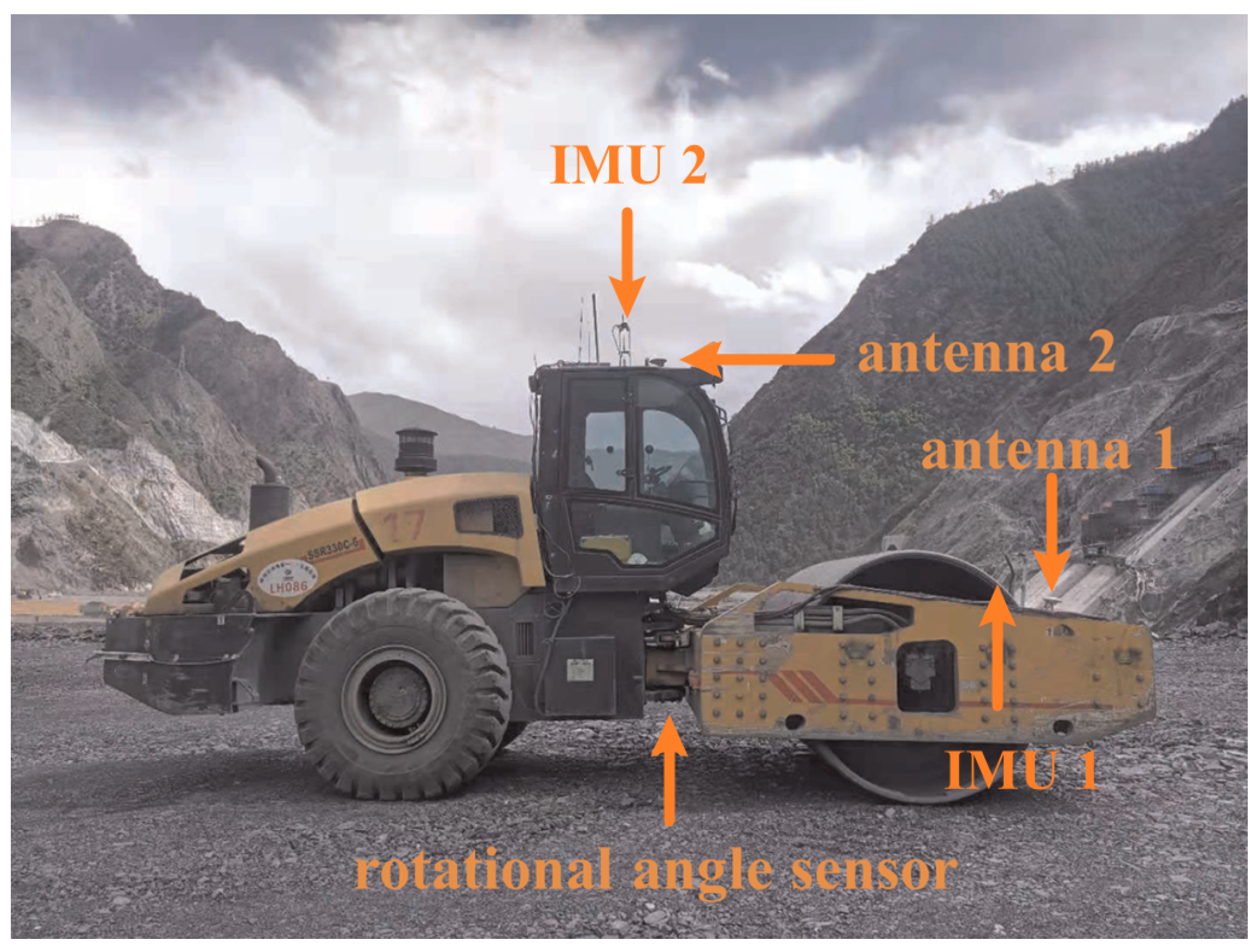
2.1. Real UR Platform

The experimental platform is a single-drum articulated UR specifically modified for autonomous operation. It features an articulated frame design, with the front drum serving as the primary compaction element and the rear wheels providing propulsion. The steering system of the UR is hydraulically driven, with two parallel hydraulic cylinders controlling the articulated angle to achieve a steering angle range of ±35 degrees.

The system design prioritizes low cost, high safety, stability, and ease of expansion to ensure efficient implementation and upgrade. The autonomous modifications of the UR include the integration of several key components to enable precise control and data acquisition. The control system is built around a real-time embedded controller utilizing Infineon’s automotive-grade chip, which offers a robust and reliable platform capable of stable operation under conditions of strong vibration and extreme conditions. As illustrated in Figure 2, a GNSS-based dual-antenna positioning system provides real-time, high-accuracy location data and heading angle, while two inertial measurement units (IMUs) measure the orientation angles (yaw, pitch, and roll), angular velocities, angular accelerations, and linear acceleration, providing a comprehensive understanding of the UR’s orientation and dynamics. A rotational angle sensor, mounted at the steering joint, measures the articulation angle between the front and rear frames. These sensors are managed and coordinated by a real-time embedded controller, which executes autonomous navigation and control algorithms in real time. All of these components are interconnected via a CAN bus for efficient and synchronized communication.

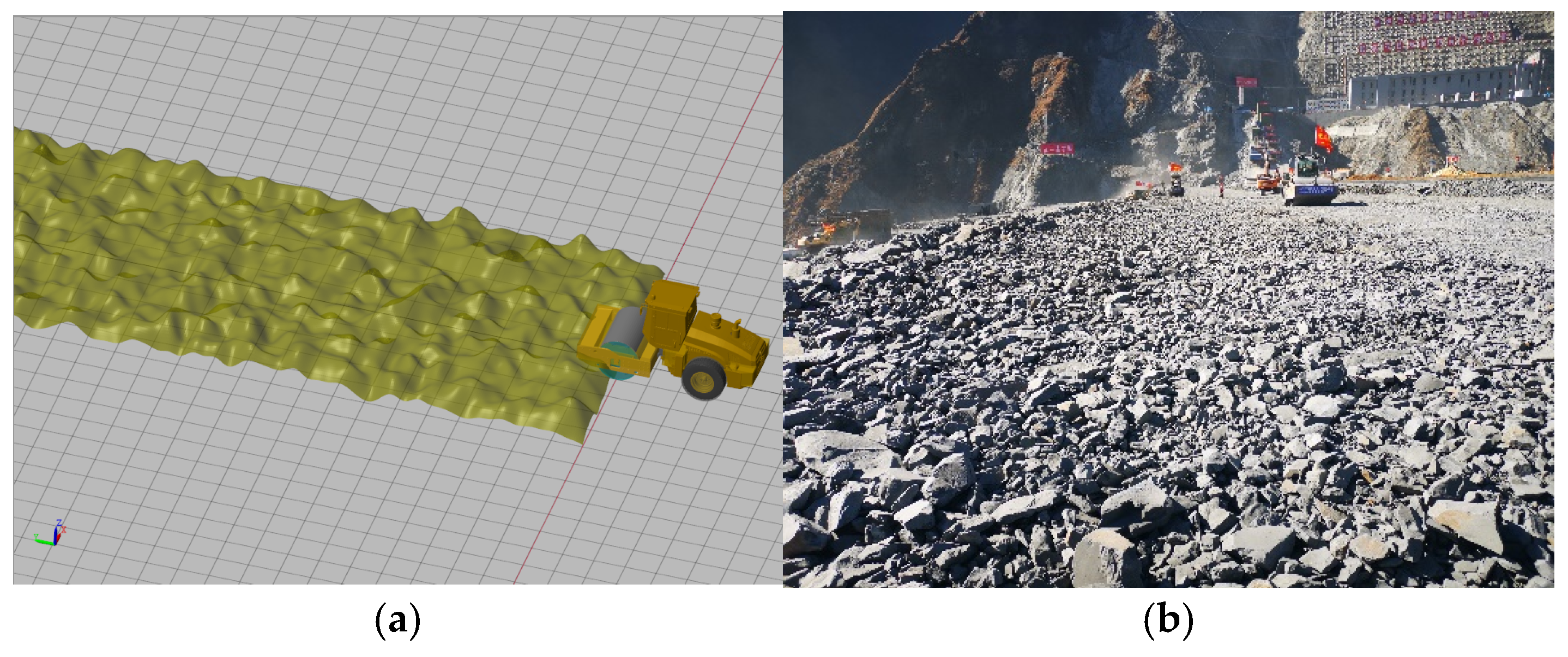
2.2. Simulation Platform

Due to the lack of mature commercial software capable of directly simulating the UR, the simulation platform was developed using non-causal modeling tools (such as OpenModelica [28] and Dymola [29]) to accurately simulate the dynamic behavior of the UR.

The simulation platform model includes key components such as the articulated frame structure, hydraulic steering system, and wheel–ground interaction, capturing the complex interactions between the roller/tire and its operating environment. Ground characteristics, including soil stiffness, damping characteristics, and terrain unevenness, were incorporated to provide a realistic representation of varying working conditions. By combining these physical and environmental parameters, this model offers high fidelity and supports comprehensive testing of control strategies under diverse scenarios, including extreme conditions that are difficult to replicate experimentally.

3. Control-Oriented Modeling

This chapter presents a six-degree-of-freedom (6-DOF) dynamic model for URs, aiming to accurately capture the roll and dynamic behavior of URs. By considering the coupling characteristics between the front and rear bodies, this model effectively reflects vehicle behavior on uneven terrains.

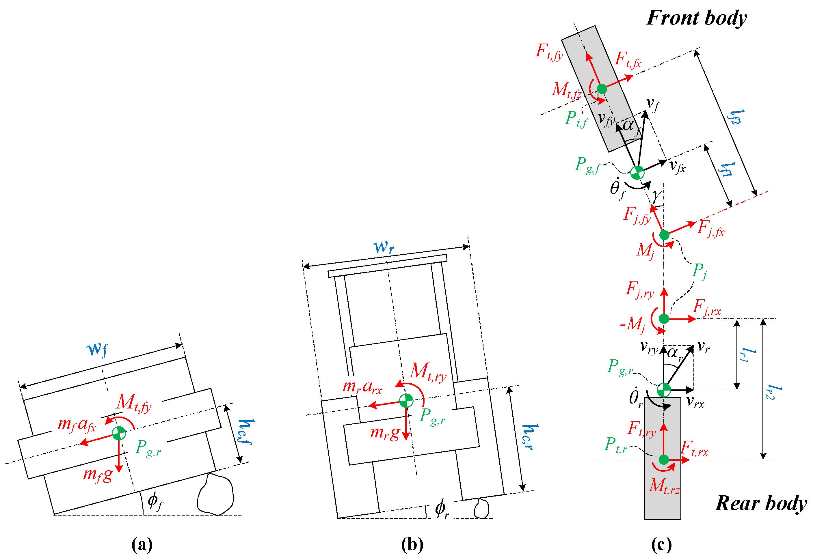
3.1. 6-DOF Dynamic Model

The proposed 6-DOF model includes two translational (longitudinal, lateral of front body), two yaw rotational (yaw of front body and articulated angle), and two roll rotational (roll angle of both bodies) degrees of freedom, the scheme of which is presented in Figure 3, and details of the variables and parameters are provided in Appendix A. In Figure 3, we denote by P_g,f and P_g,r the centers of gravity (CG) of front and rear bodies, respectively; by P_t,f and P_t,r the CGs of the front and rear axles, respectively; and by P_j the joint point that connects both bodies. The hypothesis behind the model is as follows.

• Rigid suspension hypothesis: The suspension system is assumed to have a negligible effect on vehicle dynamics. This simplification is justified by the UR’s primary application in compaction work, where a stiffer suspension is necessary to transmit larger instantaneous impact forces to the ground.
• Idealized tire-ground roll moment model: The tire-ground interaction is represented by a rotational spring-damper system to simulate the tire’s mechanical response in roll rotational directions, ignoring plastic deformation.
• Neglecting pitch dynamics: Pitch dynamics are excluded from the analysis under the assumption that their effect on overall stability is minimal. This simplification allows the model to focus on roll dynamics and reduces computational complexity.
• Single-track model assumption: The left and right wheels of each axle are simplified as a single, centralized wheel, ignoring the lateral load transfer and side force differences between them. This assumption applies exclusively to in-plane dynamics analysis.

To address the complexity introduced by the internal forces between the articulated bodies, the Lagrangian method is utilized, enabling efficient computation of the vehicle’s dynamic equations. From Figure 3c, the equilibrium equations for horizontal forces and moments acting on the entire vehicle are as follows:

$$\left\{\begin{array}{l}{m}_f{a}_{fx}\cos \gamma -m_f{a}_{fy}\sin \gamma +m_r{a}_{rx}=F_{t,fx}\cos \gamma -F_{t,fy}\sin \gamma +F_{t,rx}-m_{f}g\sin {\varphi }_f\\ m_f{a}_{fx}\sin \gamma +m_f{a}_{fy}\cos \gamma +m_r{a}_{ry}=F_{t,fx}\sin \gamma +F_{t,fy}\cos \gamma +F_{t,ry}-m_{r}g\sin {\varphi }_r\\ \left(I_{fz}+m_f{l}_{f1}^2\right){\ddot{\theta }}_f-m_f{a}_{fx}{l}_{f1}=-F_{t,fx}{l}_{f2}+m_{f}g{l}_{f1}\sin {\varphi }_f+M_j\\ \left(I_{rz}+m_r{l}_{r1}^2\right){\ddot{\theta }}_r+m_r{a}_{rx}{l}_{r1}=F_{t,rx}{l}_{r2}-m_{r}g{l}_{r1}\sin {\varphi }_r-M_j\end{array}\right.$$

(1)

In addition, the roll moment equilibrium of the front and rear bodies is influenced by inertial forces, gravitational forces, and tire–ground interaction forces. Therefore, the equilibrium equations are established as follows:

$$\left\{\begin{array}{l}{I}_{fy}{\ddot{\varphi }}_f-m_f{h}_{c,f}{a}_{fx}=-m_{f}g{h}_{c,f}\sin {\varphi }_f+M_{t,fy}\\ I_{ry}{\ddot{\varphi }}_r-m_r{h}_{c,r}{a}_{rx}=-m_{r}g{h}_{c,r}\sin {\varphi }_r+M_{t,ry}\end{array}\right.$$

(2)

The accelerations ($a_{fx},a_{fy},a_{rx},a_{ry}$) include translational acceleration and centripetal acceleration, so they can be derived as

$$\left\{\begin{array}{c}{a}_{fx}={\dot{v}}_{fx}-v_{fy}{\dot{\theta }}_f\\ a_{fy}={\dot{v}}_{fy}+v_{fx}{\dot{\theta }}_f\\ a_{rx}={\dot{v}}_{rx}-v_{ry}{\dot{\theta }}_r\\ a_{ry}={\dot{v}}_{ry}+v_{rx}{\dot{\theta }}_r\end{array}\right.$$

(3)

Considering the kinematic constraints between the states of the front and rear bodies, especially the yaw angle constraint ${\theta }_r={\theta }_f-\gamma$, the state variables of the front body and the articulated angle can be used to the rear body velocities in Equation (4).

$$\left\{\begin{array}{l}{v}_{rx}=-v_{fy}\sin \gamma +\left(v_{fx}+l_{f1}{\dot{\theta }}_f\right)\cos \gamma +l_{r1}{\dot{\theta }}_r\\ v_{ry}=v_{fy}\cos \gamma +\left(v_{fx}+l_{f1}{\dot{\theta }}_f\right)\sin \gamma \\ {\dot{v}}_{rx}=-{\dot{v}}_{fy}\sin \gamma -v_{fy}\dot{\gamma }\cos \gamma +\left({\dot{v}}_{fx}+l_{f1}{\ddot{\theta }}_f\right)\cos \gamma - \left(v_{fx}+l_{f1}{\dot{\theta }}_f\right)\dot{\gamma }\sin \gamma +l_{r1}{\ddot{\theta }}_r\\ {\dot{v}}_{ry}={\dot{v}}_{fy}\cos \gamma -v_{fy}\dot{\gamma }\sin \gamma +\left({\dot{v}}_{fx}+l_f{\ddot{\theta }}_f\right)\sin \gamma +\left(v_{fx}+l_{f1}{\dot{\theta }}_f\right)\dot{\gamma }\cos \gamma \end{array}\right.$$

(4)

Tire forces and torques of the front and rear wheels are given by the following:

$$\left\{\begin{array}{l}{F}_{t,fx}=f_{fx}\left({\alpha }_f,s_f,\mu ,F_{fz}\right)\\ F_{t,fy}=f_{fy}\left({\alpha }_f,s_f,\mu ,F_{fz}\right)\\ F_{t,rx}=f_{rx}\left({\alpha }_r,s_r,\mu ,F_{rz}\right)\\ F_{t,ry}=f_{ry}\left({\alpha }_r,s_r,\mu ,F_{rz}\right)\end{array}\right.$$

(5)

where $f_{ix}\left(\cdot \right)$ and $f_{iy}\left(\cdot \right)$ are the functions of lateral force and longitudinal force, respectively, and they are described in detail in Section 3.2. The index i represents the variables for the front body (i = f) and rear body (i = r). $F_{t,fz}$ and $F_{t,rz}$, the loads of the front and rear wheels, are equal to $m_{f}g$ and $m_{r}g$, respectively, based on Assumption 4.

In Equation (5), $s_f$ and $s_r$ are the slip ratios of the front and rear wheels, respectively. ${\alpha }_f$ and ${\alpha }_r$ are the slip angles of the front and rear wheel, respectively, representing the angle between the wheel velocity and wheel heading angle, which can be derived as follows:

$$\left\{\begin{array}{l}{\alpha }_f={\tan }^{-1}{\displaystyle \frac{v_{t,fx}}{v_{t,fy}}}\\ {\alpha }_r={\tan }^{-1}{\displaystyle \frac{v_{t,rx}}{v_{t,ry}}}\end{array}\right.$$

(6)

where $v_{t,fx}$ and $v_{t,rx}$ are the lateral velocities of the front and rear wheels, respectively, and $v_{t,fy}$ and $v_{t,ry}$ are the longitudinal velocities of the front and rear wheels, respectively. Since the wheels of UR can only roll and cannot turn, the center of gravity (CG) of the front/rear wheel and front/rear body can be considered part of a single rigid body, sharing the same motion characteristics when analyzing the motion at wheels’ CG. So, the velocities can be expressed as follows:

$$\left\{\begin{array}{l}{v}_{t,fx}=v_{fx}+\left(l_{f2}-l_{f1}\right){\dot{\theta }}_f\\ v_{t,fy}=v_{fy}\\ v_{t,rx}=v_{rx}+\left(l_{r2}-l_{r1}\right){\dot{\theta }}_r\\ v_{t,ry}=v_{ry}\end{array}\right.$$

(7)

The slip ratio quantifies the difference between the tire’s actual rolling speed and its ideal rolling speed. For the front wheel, the slip ratio s_f is defined as follows:

$$s_f=\left\{\begin{array}{l}{\displaystyle \frac{r_f{\omega }_f}{v_{t,fy}}}-1, \mathrm{if} v_{t,fy}>r_f{\omega }_f,v_{t,fy}\ne 0 \mathrm{for} \mathrm{braking} \\ 1-{\displaystyle \frac{v_{t,fy}}{r_f{\omega }_f}}, \mathrm{if} v_{t,fy}<r_f{\omega }_f,{\omega }_f\ne 0 \mathrm{for} \mathrm{driving}\end{array}\right.$$

(8)

where ${\omega }_f$ and $r_f$ are the front wheel’s angular speed and radius, respectively.

The $M_{t,fy}$ and $M_{t,ry}$ are the roll moments of the front and rear bodies, generated by vertical deformation at the tire–ground interface. Based on Assumption 2, the plastic deformation of both the ground and tires is neglected, modeling the moments as the effect of a torsional spring-damper system.

$$\left\{\begin{array}{l}{M}_{t,fy}=k_{roll,f}{\varphi }_f+c_{roll,f}{\dot{\varphi }}_f\\ M_{t,ry}=k_{roll,r}{\varphi }_r+c_{roll,r}{\dot{\varphi }}_r\end{array}\right.$$

(9)

where $k_{roll,f}$ and $k_{roll,r}$ are the torsional spring coefficients of the front body and rear body, respectively; $c_{roll,f}$ and $c_{roll,r}$ are the damping coefficients of the front body and rear body, respectively.

Using Equations (1)–(4), the dynamic model of the UR is established as follows:

$$\left\{\begin{array}{l}\dot{\mathit{x}}=f\left(\mathit{x},\mathit{u}\right)\\ \mathit{y}=\mathit{C}\mathit{x}\end{array}\right.$$

(10)

where the state vector is $\mathit{x}={\left[\begin{array}{ccccccccc}{v}_{fx}& v_{fy}& {\dot{\theta }}_f& \dot{\gamma }& \gamma & {\varphi }_f& {\varphi }_r& X_f& Y_f\end{array}\right]}^T$, $\mathit{u}=M_j$, $\mathit{C}=\left[\begin{array}{cc}{\mathit{I}}_2& {\mathbf{0}}_{2\times 7}\end{array}\right]$, $f\left(\mathit{x},\mathit{u}\right)$ denotes the nonlinear function, which is expressed in Appendix B.

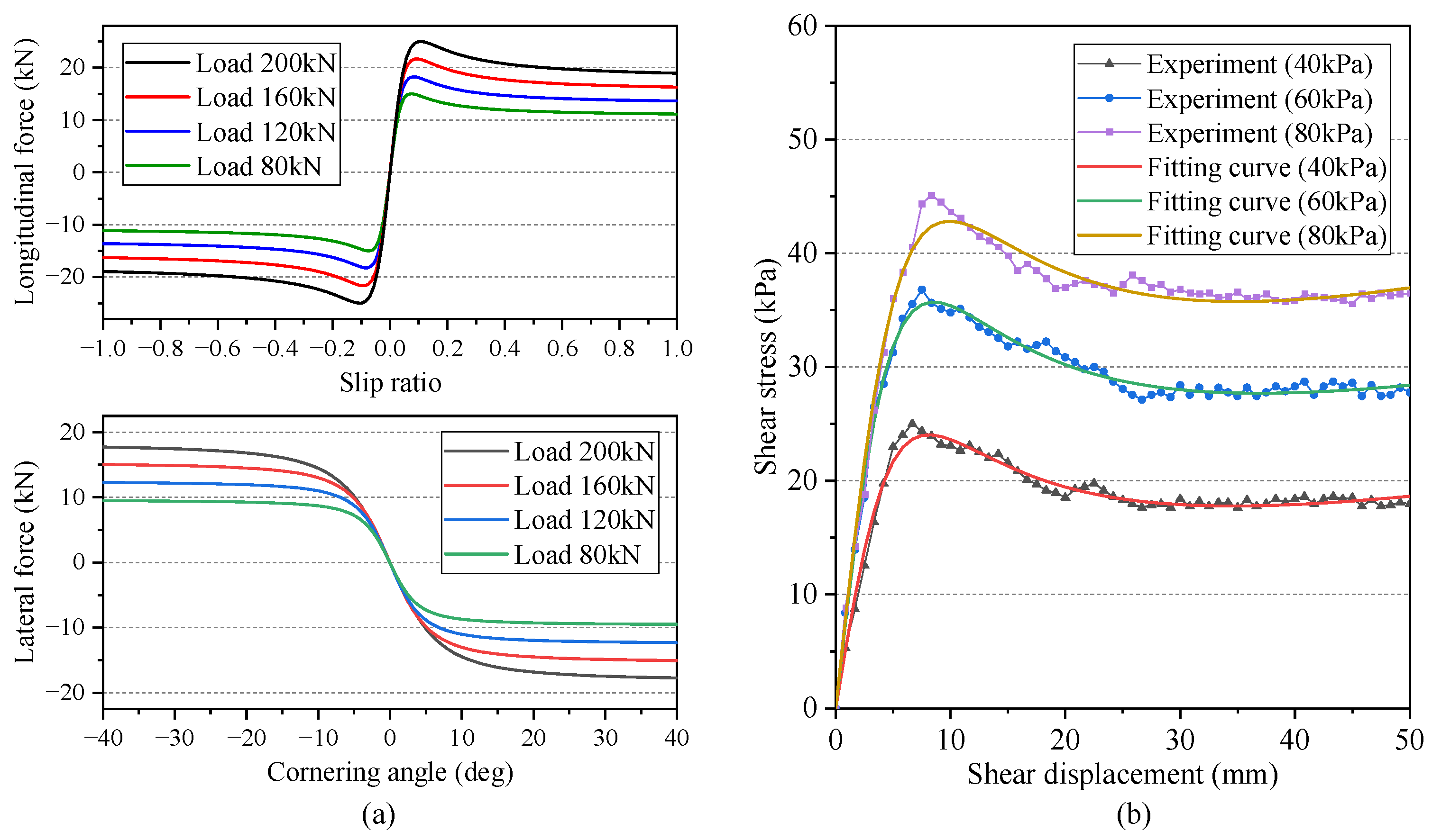
3.2. Rear Tires and Front Drum Model

The Magic Formula (MF) [30,31] is a widely used semi-empirical model capable of describing the traction and lateral force characteristics of tires. The MF relates the longitudinal and lateral forces of a tire to variables such as slip ratio and sideslip angle through a series of parametric equations. It effectively captures the interaction between traction and sideslip forces under combined conditions, including steering, braking, and driving.

Figure 4a illustrates the lateral and longitudinal forces as functions of the cornering angle and slip ratio under varying tire loads. Unlike conventional rubber tires, the front drum of the UR is made of steel, which exhibits negligible elastic rebound characteristics. This poses a challenge when directly applying the MF to describe the front drum’s behavior. To address this issue, prior studies have investigated the shear stress characteristics of steel–rock interactions [32,33,34,35,36,37]. Figure 4b illustrates the experimental data [37] for steel–rock contact surfaces, which were fitted to the Magic Formula. The resulting fit achieved an average correlation coefficient of 0.992, demonstrating that the MF effectively captures the nonlinear mechanical characteristics arising from plastic deformation, sliding, and particle rearrangement at the interface. Considering that the contact between the URs’ front drum and the ground can be regarded as a macroscopic representation of metal–sandstone interactions, the nonlinear contact mechanics between the front drum and the rock surface can also be accurately described by the MF.

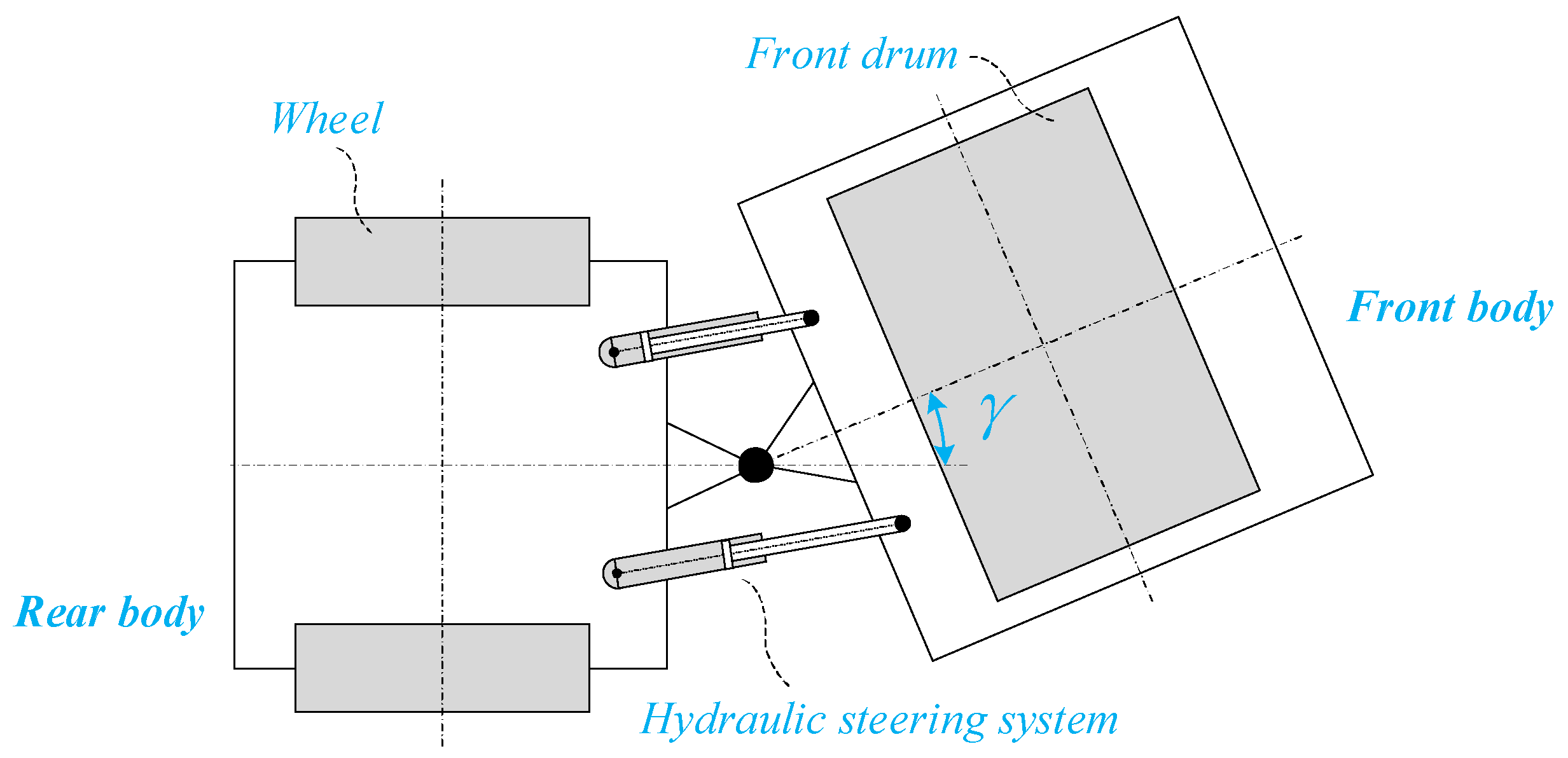
3.3. Hydraulic Steering Model

The hydraulic steering system is illustrated in Figure 5. The hydraulic pump pressurizes the hydraulic oil from $p_0$ to $p_s$. The pressurized oil is then delivered to a 3-position, 4-way directional control valve, the opening of which ($A_v$) and connected flow paths are regulated by the steering input.

In Figure 5, Line 1 is connected to the supply line, and Line 2 to the return line, with flow rates $q_1$ and $q_2$, respectively. When hydraulic oil flows into hydraulic cylinders, it drives the pistons, generating mechanical force. The relief valve prevents the pressure in the hydraulic lines from exceeding the designated threshold. The check valve, on the other hand, prevents the backflow of hydraulic oil.

The change rate of steering torque ${\dot{M}}_j$ is generated by the hydraulic forces and is expressed as follows:

$${\dot{M}}_j={\dot{F}}_r{l}_{h,r}-{\dot{F}}_l{l}_{h,l}$$

(11)

where $l_{h,l}$ and $l_{h,r}$ are the vertical distance from joint $P_j$ to the left and right piston rods. The hydraulic forces $F_l$ and $F_r$ acting on the left and right piston rods are determined by the pressure differences within the piston chambers and are given by the following:

$$\left\{\begin{array}{l}{\dot{F}}_l\left(t\right)={\dot{p}}_2{A}_p-{\dot{p}}_1\left(A_p-A_r\right)\\ {\dot{F}}_r\left(t\right)={\dot{p}}_1{A}_p-{\dot{p}}_2\left(A_p-A_r\right)\end{array}\right.$$

(12)

where $A_p$ is the piston area and $A_r$ is the rod area. The dynamic of pressure $p_1$ and $p_2$ in the left and right chambers are influenced by the volume flow, chamber volume change, and hydraulic oil leakage. These dynamics are described by the following equations:

$$\left\{\begin{array}{ll}{\dot{p}}_1\left(t\right)& =f_{p1}\left(A_v,{\dot{l}}_{hy,l},{\dot{l}}_{hy,r}\right)\\ & ={\displaystyle \frac{K_{oil}}{V_1}}\left(-c_d{A}_v\sqrt{p_1-p_0}-2k_{leak}\left(p_1-p_2\right)-A_p{\dot{l}}_{hy,l}+A_r{\dot{l}}_{hy,r}\right)\\ {\dot{p}}_2\left(t\right)& =f_{p2}\left(A_v,{\dot{l}}_{hy,l},{\dot{l}}_{hy,r}\right)\\ & ={\displaystyle \frac{K_{oil}}{V_2}}\left(c_d{A}_v\sqrt{p_s-p_2}+2k_{leak}\left(p_1-p_2\right)+A_r{\dot{l}}_{hy,l}-A_p{\dot{l}}_{hy,r}\right)\end{array}\right.$$

(13)

where $K_{oil}$ is the fluid bulk modulus of hydraulic oil; and $V_1$ and $V_2$ are the volumes of the cylinder chambers connected to Line 1 and Line 2, respectively. $c_d$ is the flow coefficient. $A_v$ is the opening of a 3-position, 4-way directional control valve. $k_{leak}$ is the leakage coefficient. $l_{hy,l}$ and $l_{hy,r}$ are the lengths of the left and right cylinders.

4. Rollover Energy Barrier

The rollover energy barrier (REB) serves as a critical metric for evaluating the safety of articulated vehicles. It quantifies the energy barrier separating the vehicle’s current state (see Figure 6b) from its critical rollover state (see Figure 6a), offering a direct measure of rollover risk. A higher REB value signifies that the vehicle needs more energy from rollover, which means greater rollover stability and safety.

Figure 6b shows the state variables influencing the REB in the general state, which represent the contributions of potential energy and kinetic energy. The REB can thus be expressed as follows:

$$RE{B}_i=\left\{\begin{array}{ll}RE{B}_{c,i}-E_{p,i}-E_{k,i},& \left|{\varphi }_i\right|<\left({\displaystyle \frac{\pi }{2}}-{\sigma }_i\right)\\ RE{B}_{c,i},& \left|{\varphi }_i\right|>\left({\displaystyle \frac{\pi }{2}}-{\sigma }_i\right)\end{array}\right.$$

(14)

where $RE{B}_{c,i}$ is the potential energy of the critical rollover state, the $E_{p,i}$ is the generalized roll potential energy, and the $E_{k,i}$ is the roll kinetic energy. Neglecting the energy absorption of the roll limit block during the roll energy transfer between the front and rear bodies, the REB of the vehicle can be defined as follows:

$$REB=RE{B}_f+RE{B}_r$$

(15)

4.1. The Critical Rollover Energy

Figure 6a illustrates the critical rollover state, that is, the vertical projection of the CG coincides with the wheel support point. In this state, both roll angular velocity and angular acceleration are zero, and the potential energy reaches its critical rollover value $RE{B}_{c,i}$. Considering that the critical rollover height of CG is $\sqrt{w_i^2/4+h_{c,i}^2}$, the $RE{B}_{c,i}$ can be obtained as follows:

$$RE{B}_{c,i}=m_{i}g\sqrt{{\displaystyle \frac{w_i^2}{4}}+h_{c,i}^2}$$

(16)

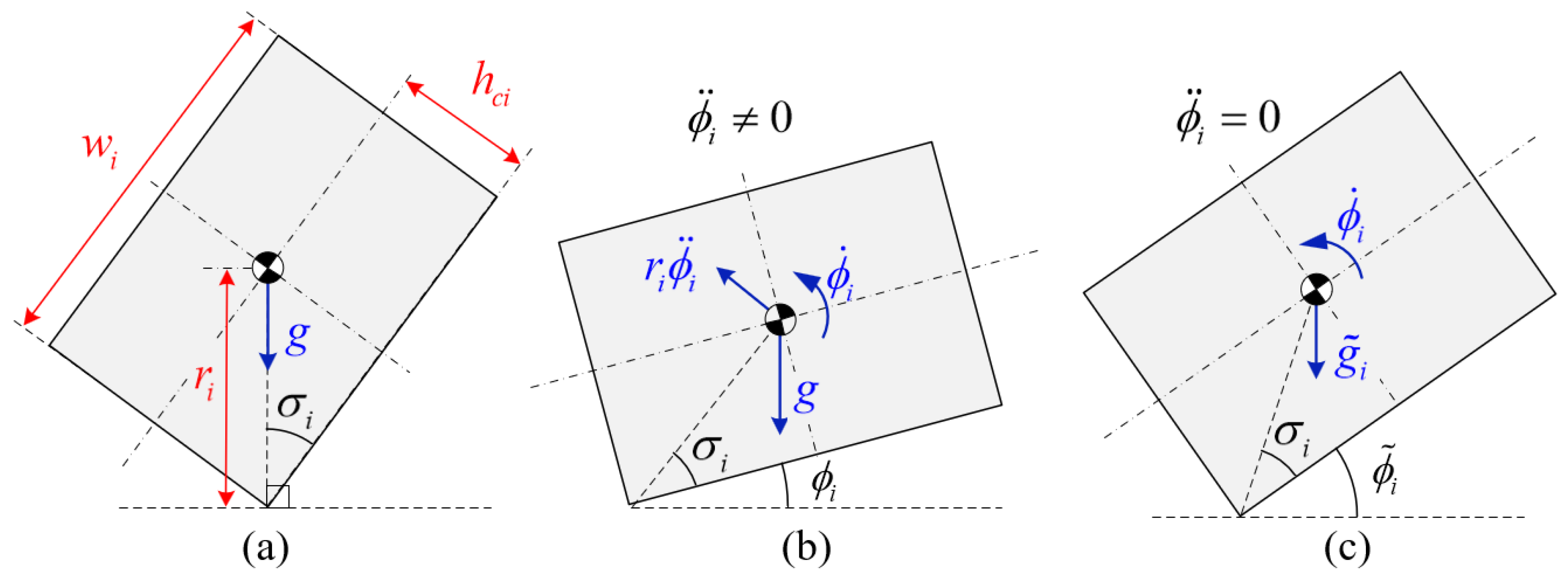
4.2. Generalized Potential Energy

In addition to the potential energy generated by gravitational acceleration $g$, the roll tangential acceleration $r_i{\ddot{\varphi }}_i$ in the x–z plane plays a significant role in influencing tripped rollover risk. To comprehensively evaluate the impact of $r_i{\ddot{\varphi }}_i$ and $g$ on rollover risk, the concept of virtual gravitational acceleration (VGA) is introduced. The VGA unifies these two components within a generalized potential energy framework, simplifying the analysis of rollover dynamics.

The VGA ${\tilde{g}}_i$ is defined as the vector sum of the gravitational and roll tangential accelerations. This reconfiguration transforms Figure 6b into Figure 6c, and the magnitude of ${\tilde{g}}_i$ is expressed as follows:

$${\tilde{g}}_i=\sqrt{{\left(g\sin {\varphi }_i+r_i{\ddot{\varphi }}_i\sin {\sigma }_i\right)}^2+{\left(g\cos {\varphi }_i+r_i{\ddot{\varphi }}_i\cos {\sigma }_i\right)}^2}$$

(17)

where ${\sigma }_i=\arctan \left(2h_{ci}/w_i\right)$, $r_i=\sqrt{h_{ci}^2+w_i^2/4}$.

The artificial roll angle ${\tilde{\varphi }}_i$ can be derived as follows:

$${\tilde{\varphi }}_i=\arctan {\displaystyle \frac{g\sin {\varphi }_i+r_i{\ddot{\varphi }}_i\sin {\sigma }_i}{g\cos {\varphi }_i-r_i{\ddot{\varphi }}_i\cos {\sigma }_i}}$$

(18)

In Figure 6c, the height of the virtual CG is $\left(0.5w_i\sin {\tilde{\varphi }}_i+h_{ci}\cos {\tilde{\varphi }}_i\right)$, so the generalized potential energy $E_{p,i}$ is given by

$$E_{p,i}=m_i{\tilde{g}}_i\left({\displaystyle \frac{w_i}{2}}\sin {\tilde{\varphi }}_i+h_{ci}\cos {\tilde{\varphi }}_i\right)$$

(19)

4.3. Roll Kinetic Energy

Roll kinetic energy is related to roll tangential acceleration $r_i{\ddot{\varphi }}_i$, and its rotation center is the support point of the wheel on the ground. So, the roll kinetic energy is given by

$$E_{p,i}={\displaystyle \frac{1}{2}}{I}_y^{\prime }{\dot{\varphi }}_i^2$$

(20)

where $I_{iy}^{\prime }=I_{iy}+m_i{r}_i^2$ is the moment of inertia of the vehicle bodies with the supposed point as the center of rotation.

5. Hierarchical Controller Design

The hierarchical stability controller (HSC), as illustrated in Figure 7, comprises a high-level planner and a low-level controller, responsible for a feasible anti-rollover trajectory generation and motion control, respectively.

The high-level planner employs NMPC to generate feasible trajectories [38], which are executed by the low-level controller. These trajectories are designed to satisfy the vehicle’s dynamic constraints, steering torque change rate limit, with low rollover risk.

The low-level controller adopts a cascaded disturbance rejection control strategy [39,40] based on ADRC [41] to achieve precise tracking of the target trajectory. This method strikes a balance between computational efficiency and control accuracy, ensuring reliable real-time performance [40].

5.1. High-Level NMPC

The high-level planner employs an NMPC to replan a feasible reference trajectory that aligns with the UR’s dynamic characteristics, specifically minimizing the rollover risk. Due to the complexity of the hydraulic steering system, which imposes a significant computational burden, the NMPC reference model simplifies the input by using hydraulic steering torque instead of steering angle. This approach eliminates the need to model the hydraulic steering system. Nevertheless, to ensure trajectory feasibility and comply with the physical constraint of UR’s steering torque, the change rate of the hydraulic steering torque is incorporated as a constraint in NMPC. This approach balances computational efficiency with trajectory executability.

The continuous-time model (Equation (10)) is discretized using a sampling interval $\Delta t$, resulting in the following discrete-time formulation:

$${\mathit{x}}_{k+1}={\mathit{x}}_k+\Delta t\cdot f\left({\mathit{x}}_k,{\mathit{u}}_k\right)$$

(21)

where the index k, k + 1, and k + m in the following sections, respectively, donate the predicted value at the k, k + 1, and k + m step.

To constrain the steering torque change rate, ${\mathit{u}}_k$ is replaced by its increment $\Delta {\mathit{u}}_k$, leading to a reformulation of Equation (21) as follows:

$$\left\{\begin{array}{l}{\xi }_{k+1}={\xi }_k+\Delta t\cdot g\left({\xi }_k,\Delta {\mathit{u}}_k\right)\\ {\mathit{y}}_k=\tilde{\mathit{C}}{\xi }_k\end{array}\right.$$

(22)

where $\Delta \mathit{u}=\Delta M_j=\Delta t\cdot {\dot{M}}_j$, and ${\dot{M}}_j$ is derived from Formula (11). The new state variable vector $\xi$ is formed as $\xi =[\begin{array}{cc}u& M_j\end{array}]$, which yields $\tilde{\mathit{C}}=\left[\begin{array}{cc}\mathit{C}& {\mathbf{0}}_{2\times 1}\end{array}\right]$.

The cost function is designed to track the reference path and reduce the risk of rollover while optimizing the control rate to ensure lateral stability. So, the cost function can be expressed as follows:

$$\begin{array}{l}J\left({\mathit{y}}_k,\Delta {\mathit{u}}_k,RE{B}_k\right)=\begin{array}{l}{\displaystyle \sum _{m=1}^{N_p}\left({‖{\mathit{y}}_{k+m}‖}_Q^2+{‖RE{B}_{c,f}+RE{B}_{c,r}-RE{B}_{k+m}‖}_S^2\right)}+{\displaystyle \sum _{m=1}^{N_c}{‖\Delta {\mathit{u}}_{k+m}‖}_R^2}\hfill \end{array}\hfill \end{array}$$

(23)

where N_p and N_c are the predictive horizon and control horizon, respectively, and Q, R, and S are positive semidefinite, representing the relative importance of each term.

Over the N_p-step prediction horizon, the following optimal control problem is solved at each time step:

$$\begin{array}{l}\begin{array}{l}\min J\left({\mathit{y}}_k,\Delta {\mathit{u}}_k,RE{B}_k\right)\hfill \end{array}\hfill \\ s.t. \left\{\begin{array}{l}{\xi }_{k+1}={\xi }_k+\Delta T\cdot g\left({\xi }_k,\Delta {\mathit{u}}_k\right)\\ {\xi }_{\min }\le {\xi }_{k+j}\le {\xi }_{\max }\\ \Delta M_{j,\min }\le \Delta M_{j,k}\le \Delta M_{j,\max }\end{array}\right.\hfill \end{array}$$

(24)

where $\Delta M_{j,\max }=-\Delta M_{j,\min }$, which can be derived from Equation (11) by assuming $\dot{\gamma }$ and $A_v$ reach their maximum limits.

The nonlinear optimization problem (Equation (24)) is solved using a Sequential Quadratic Programming method. This approach iteratively linearizes the constraints and approximates the objective function quadratically, enabling the solution of a series of quadratic programming subproblems [42]. The implementation utilizes solver CasADi [43] for the efficient computation of gradients and Hessians. Solving the optimization problem yields the optimal control sequence:

$${\mathit{u}}^{*}=\left\{u_{k+m}^{*}|m=0,1,2,\dots ,N_c\right\}$$

(25)

By substituting the optimized control sequence ${\mathit{u}}^{*}$ into the discrete dynamic model (Equation (22)), the resulting optimal tracking trajectory set $\mathcal{P}$ with low rollover risk can be expressed as

$$\mathcal{P}=\left\{{\left(X_{ref}^{*},Y_{ref}^{*}\right)}_{k+m}|m=1,2,3,\dots ,N_p\right\}$$

(26)

5.2. Low-Level CDRC

In the low-level controller, a cascaded disturbance rejection control (CDRC) strategy is designed to enhance the system’s tracking and disturbance rejection performance. As depicted in Figure 7, the cascaded structure consists of an outer loop for lateral error tracking and an inner loop for heading error (HE) tracking. In addition, two extended state observers (ESOs) are designed for disturbance estimation and model compensation. In previous studies [39,40], by leveraging the CDRC framework, the controller actively estimates and compensates for system uncertainties and external disturbances, ensuring robust and precise control under varying operating conditions.

The classic articulated vehicle kinematic models [44] of heading angle and lateral error are

$$\left\{\begin{array}{l}{\dot{\theta }}_f={\displaystyle \frac{v_f\sin \gamma }{l_f\cos \gamma +l_r}}+{\displaystyle \frac{\dot{\gamma }{l}_f}{l_f\cos \gamma +l_r}}\\ {\dot{e}}_{CTE}=v_f\sin \left({\theta }_f-{\theta }_{ref}\right)\end{array}\right.$$

(27)

The dynamics of the steering system are approximated by a simple linear system, i.e., $\dot{\gamma }=\left(-\gamma +k_s\delta +b_s\right)/\tau$, enabling the heading angle model as

$${\dot{\theta }}_f={\displaystyle \frac{\tau v_f\sin \gamma -\gamma l_r+b_s{l}_r}{\tau \left(l_f\cos \gamma +l_r\right)}}+{\displaystyle \frac{k_s{l}_r\delta }{\tau \left(l_f\cos \gamma +l_r\right)}}$$

(28)

where $\delta$ is the steering wheel angle, and $k_s$, $b_s$, and $\tau$ are, respectively, the slope, intercept, and time constant from the steer motor angle to the articulated angle.

The CDRC lumped all the discrepancies in the kinematic model [44] into the outer-loop and inner-loop total disturbance, $f_{ol}$ and $f_{il}$, respectively. Hence, the extended state model of heading angle is rewritten as follows:

$$\left\{\begin{array}{l}{\dot{\theta }}_f=f_{0,il}+b_{0,il}{\delta }_{cmd}+f_{il}\\ {\dot{f}}_{il}=h\end{array}\right.$$

(29)

where ${\delta }_{cmd}$ is the final output of CDRC, and h, an unknown variable, is the derivative of the total disturbance $f_{il}$. $b_{0,il}$ and $f_{0,il}$ can be expressed as follows:

$$\left\{\begin{array}{l}{b}_{0,il}={\displaystyle \frac{k_s{l}_r}{\tau \left(l_f\cos \gamma +l_r\right)}}\hfill \\ f_{0,il}={\displaystyle \frac{\tau v_f\sin \gamma -\gamma l_r+b_s{l}_r}{\tau \left(l_f\cos \gamma +l_r\right)}}+{\displaystyle \frac{k_s{l}_r{\delta }_{cmd}}{\tau \left(l_f\cos \gamma +l_r\right)}}\hfill \end{array}\right.$$

(30)

Then, Equation (29) can be rewritten as a state space model as follows.

$$\left\{\begin{array}{l}{\dot{X}}_{il}=A_{il}{X}_{il}+B_{il}{U}_{il}+E_{il}{f}_{0,il}+G_{il}h\hfill \\ Y_{il}=C_{il}{X}_{il}\hfill \end{array}\right.$$

(31)

where $X_{il}=\left[\begin{array}{l}{\theta }_f\hfill \\ f_{il}\hfill \end{array}\right]$, $A_{il}=\left[\begin{array}{ll}0\hfill & 1\hfill \\ 0\hfill & 0\hfill \end{array}\right]$, $B_{il}=\left[\begin{array}{l}{b}_{0,il}\hfill \\ 0\hfill \end{array}\right]$, $C_{il}=\left[\begin{array}{ll}1\hfill & 0\hfill \end{array}\right]$, $U_{il}=\left[{\delta }_{cmd}\right]$, $Y_{il}=\left[{\theta }_f\right]$, $G_{il}=\left[\begin{array}{l}0\hfill \\ 1\hfill \end{array}\right]$. To obtain the unknown disturbance $f_{il}$, the following extended state observer is designed based on state space (31).

$$\left\{\begin{array}{l}{\dot{X}}_{il}=A_{il}{X}_{il}+B_{il}{U}_{il}+E_{il}{f}_{0,il}+G_{il}h\hfill \\ Y_{il}=C_{il}{X}_{il}\hfill \end{array}\right.$$

(32)

where $L_{il}={\left[\begin{array}{cc}{\beta }_{il1}& {\beta }_{il2}\end{array}\right]}^T$ is a parameter matrix that adjusts the performance of ESO. Thus, the estimated disturbance ${\widehat{f}}_{il}$ can be obtained. Then, the inner-loop control is designed as

$${\delta }_{cmd}={\displaystyle \frac{k_{p,il}\left({\theta }_{ref,il}-{\theta }_f\right)-f_{0,il}-{\widehat{f}}_{il}+{\dot{\theta }}_{ref,il}}{b_{0,il}}}.$$

(33)

where $k_{p,il}$ is the proportional gain of the low-level controller to be tuned, and ${\theta }_{ref,il}$ is the reference orientation for the inner-loop controller and output by the outer-loop controller. Equation (33) enforces the plant in Equation (29) to behave as an integrator as follows:

$${\dot{\theta }}_f=k_{p,il}\left({\theta }_{ref,il}-{\theta }_f\right)+{\dot{\theta }}_{ref,il}$$

(34)

So far, the inner-loop controller design has been completed. Similar to the design of the inner-loop controller, the outer-loop controller can be designed based on Equation (27) as

$${\theta }_{ref,il}={\theta }_{ref}+{\sin }^{-1}\left({\displaystyle \frac{-k_{ol}{e}_{CTE}-{\widehat{f}}_{ol}}{b_{0,ol}}}\right)$$

(35)

The feasibility and stability of the CDRC are well proved in previous research [39,40], showing high trajectory tracking accuracy and robustness under complex road conditions.

6. Experimental Verification

This chapter evaluates the proposed anti-rollover solution through experiments conducted under different scenarios. The REB is compared with traditional indices to highlight its advantages in predicting rollover risks. Following this, the chapter evaluates the HSC based on REB, focusing on its effectiveness in mitigating rollover risks under uneven scenarios.

6.1. Validation of REB

The proposed REB is evaluated and compared with two widely used rollover risk indices: the Load Transfer Ratio (LTR) [10,18] and the Critical Lateral Acceleration (CLA) [8,45], due to their widespread use in rollover risk evaluation. The experimental conditions include two distinct scenarios selected for evaluation:

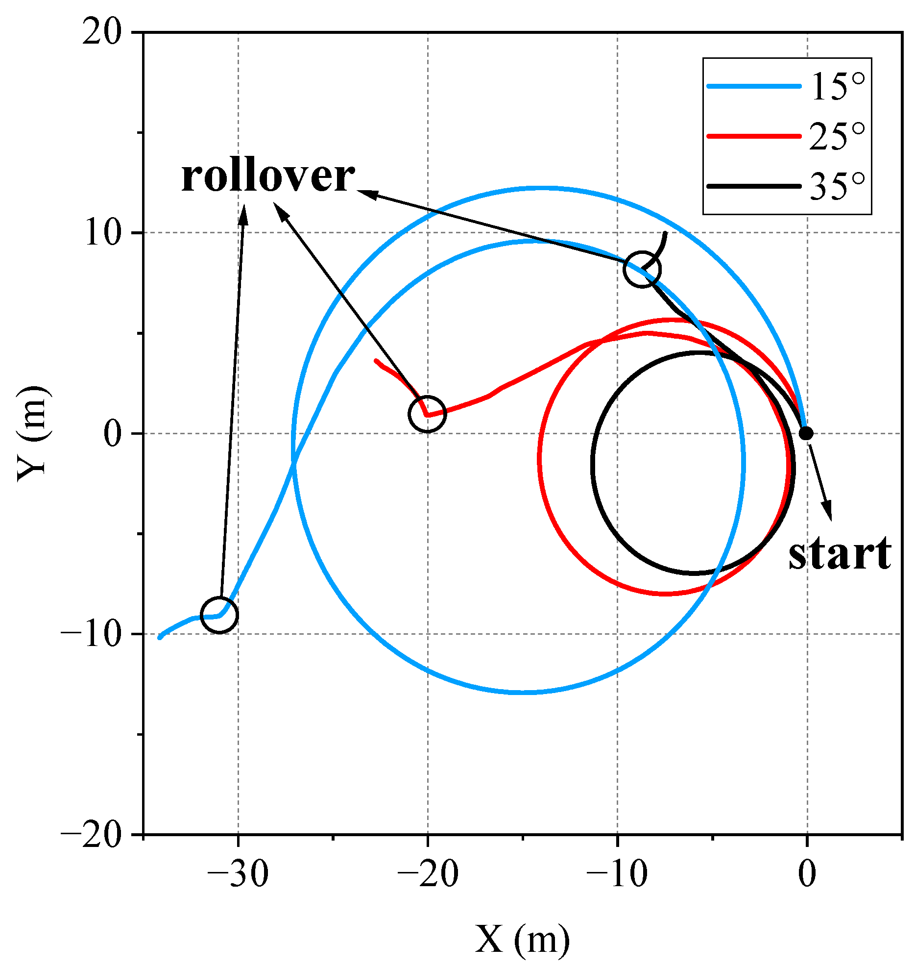
• Untripped Rollover: This scenario simulates the lateral moment imbalance caused by improper operations. In the experiment, a non-zero articulated angle remains constant, while the UR’s longitudinal speed increases linearly, ultimately leading to rollover.
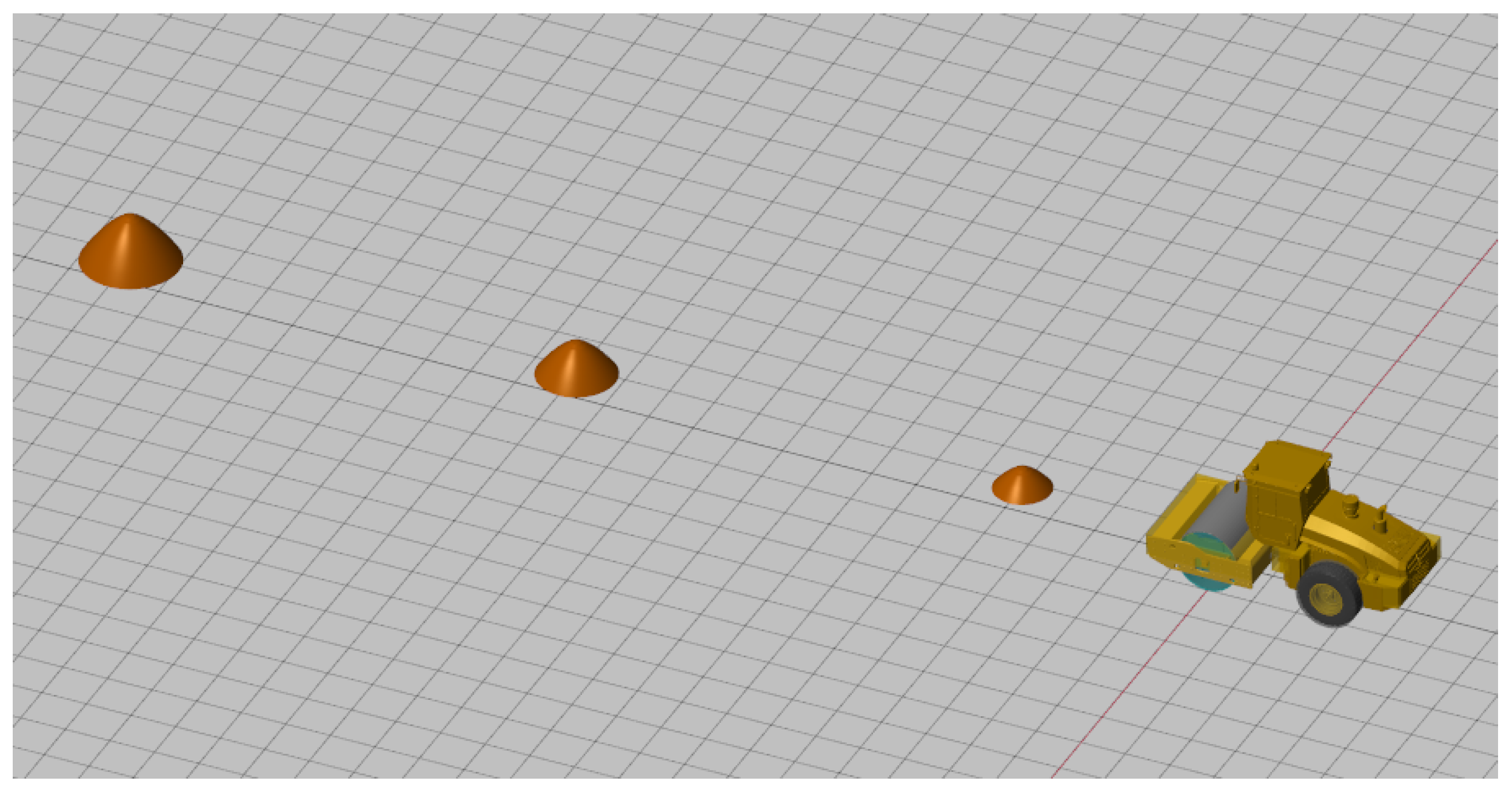
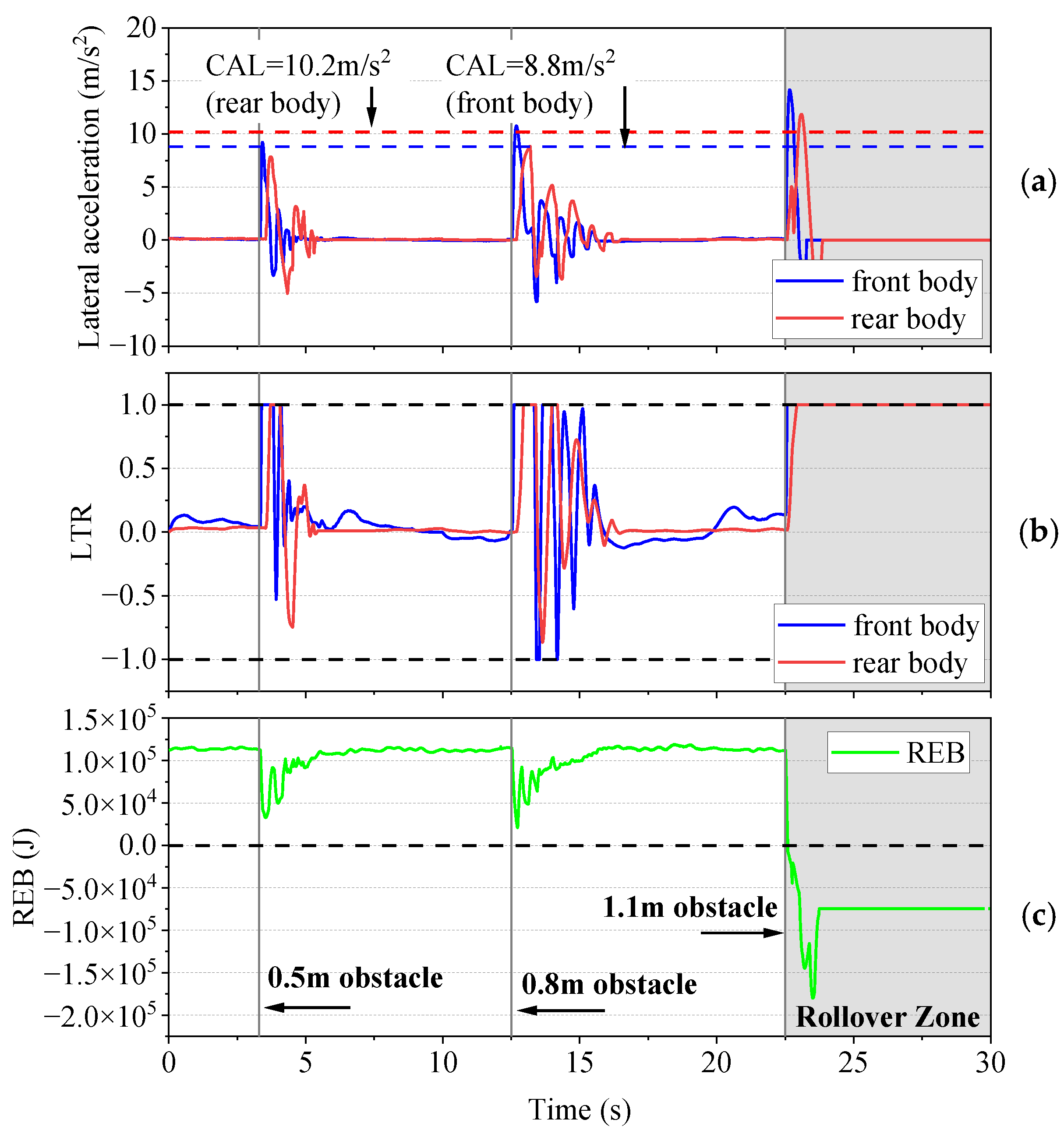
• Tripped rollover: This scenario simulates sudden vertical disturbances to the front drum and rear tires caused by ground irregularities, represented as three predefined obstacle heights within the simulation environment.

6.1.1. Untripped Rollover Scenario

In this scenario, three experiments were conducted with articulated angles of 15°, 25°, and 35°, while the longitudinal velocity of the UR increased at a constant acceleration of 1 m/s² until rollover occurred. Figure 8 illustrates the trajectories, showing that the UR’s critical rollovers occurred at 16.33 s, 12.31 s, and 9.15 s, respectively. The results are shown in Figure 9. The bold dashed lines in each subplot represent the critical rollover threshold, beyond which the state is considered unstable. The intersection points of the bold dashed lines with the respective indicator curves are identified as the warning points, marked by black circles in Figure 9. The time between the warning points and the actual occurrence of rollover is defined as the lead time, which is summarized in

Table 1. Prediction lead time of untripped rollover.

Indicators	Prediction Lead Time (s)
	15°	25°	35°	Average
CLA	--	0.21	0.35	0.280
LTR	0.36	0.46	0.53	0.450
REB	0.30	0.56	0.59	0.483

.

As shown in Figure 9a, the CLA values for the front and rear bodies are 8.8 m/s² and 10.2 m/s², respectively. The true rollover threshold acceleration increases as the articulated angle decreases. Consequently, the CLA fails to predict rollover at a 35° articulated angle and demonstrates the shortest lead time among the three indices, at just 0.280 s.

An absolute LTR value of 1.0 indicates that the entire vehicle load has shifted to one wheel, signaling an imminent rollover. As illustrated in Figure 9b, LTR accurately predicts rollover risk in all three experiments, achieving an average lead time of 0.450 s before rollover occurs.

For the REB, a value below zero signifies that the UR’s rollover energy has exceeded the threshold, indicating a significant rollover risk. As shown in Figure 9c, the REB effectively predicts all three rollover risks, achieving the longest average lead time of 0.483 s.

6.1.2. Tripped Rollover Scenario

In the tripped rollover experiment, considering the complexity of real-world conditions (such as surface materials, bump shapes, and dynamic impacts), the experiment was designed to select the steepest possible slope and the material with the highest elastic modulus, while ensuring the possibility that, specifically, the UR moves along a straight path with three obstacles of varying heights (0.5 m, 0.8 m, and 1.1 m) positioned on the right side to generate a leftward roll moment, as shown in Figure 10. To accurately simulate the mechanical properties of the ground, the ground parameters were selected as follows: a stiffness of 4.5 × 10⁸ N/m², a damping coefficient of 9.5 × 10⁵ Ns/m, and a friction coefficient of 0.75 (under dry conditions). It is noteworthy that the UR stabilizes after brief disturbances at the 0.5 m and 0.8 m obstacles, while excessive excitation at the 1.1 m obstacle causes rollover. The experimental results are presented in Figure 11, and the bold dashed lines, as the Figure 9, represent the critical rollover thresholds in each subplot.

As illustrated in Figure 11a, at the 0.5 m and 0.8 m obstacles, the lateral acceleration of the front body exceeds 8.8 m/s², incorrectly signaling rollover risks and demonstrating over-sensitivity, whereas the rear body’s lateral acceleration remains below the 10.2 m/s² threshold. This reveals CLA’s inability to adapt to dynamic responses under varying excitations and its failure to comprehensively evaluate the rollover risk of the UR’s dual-body structure.

For LTR, as shown in Figure 11b, frequent wheel lift-offs caused by uneven terrain repeatedly drive the LTR to its ±1 threshold, reflecting its inability to distinguish true rollover risks from transient disturbances, significantly limiting its applicability in tripped rollover scenarios.

In contrast, REB demonstrates superior adaptability and accuracy as seen in Figure 11c. At the 0.5 m and 0.8 m obstacles, REBs remain positive, indicating the vehicle maintains stability and avoids false alarms. In contrast, at the 1.1 m obstacle, REB rapidly drops below zero, signaling that the rollover threshold has been exceeded and a rollover has occurred.

In the two sets of experiments above, REB effectively addresses the rollover coupling between the front and rear bodies of articulated vehicles by quantifying rollover energy, enabling a unified evaluation of rollover risk. It demonstrates clear advantages, including earlier warning times and fewer false alarms. In contrast, LTR and CLA inherently fail to account for the coupling between the dual-body structure, as they can only assess the rollover risk of a single body, limiting their performance in articulated vehicle risk assessments. Moreover, CLA struggles to adapt to dynamic changes under varying excitations, restricting its predictive accuracy. In the tripped rollover experiment, the frequent occurrence of brief wheel lift-off causes LTR to repeatedly hit the warning threshold, increasing false alarms and significantly limiting its effectiveness.

6.2. Validation of HSC

To validate the effectiveness and advantages of the proposed HSC, this section presents a comprehensive evaluation through both simulation and real UR experiments in uneven terrain scenarios. As shown in Figure 12, the scenarios illustrate sections of bumpy roads in both the simulation environment and real-world experiments.

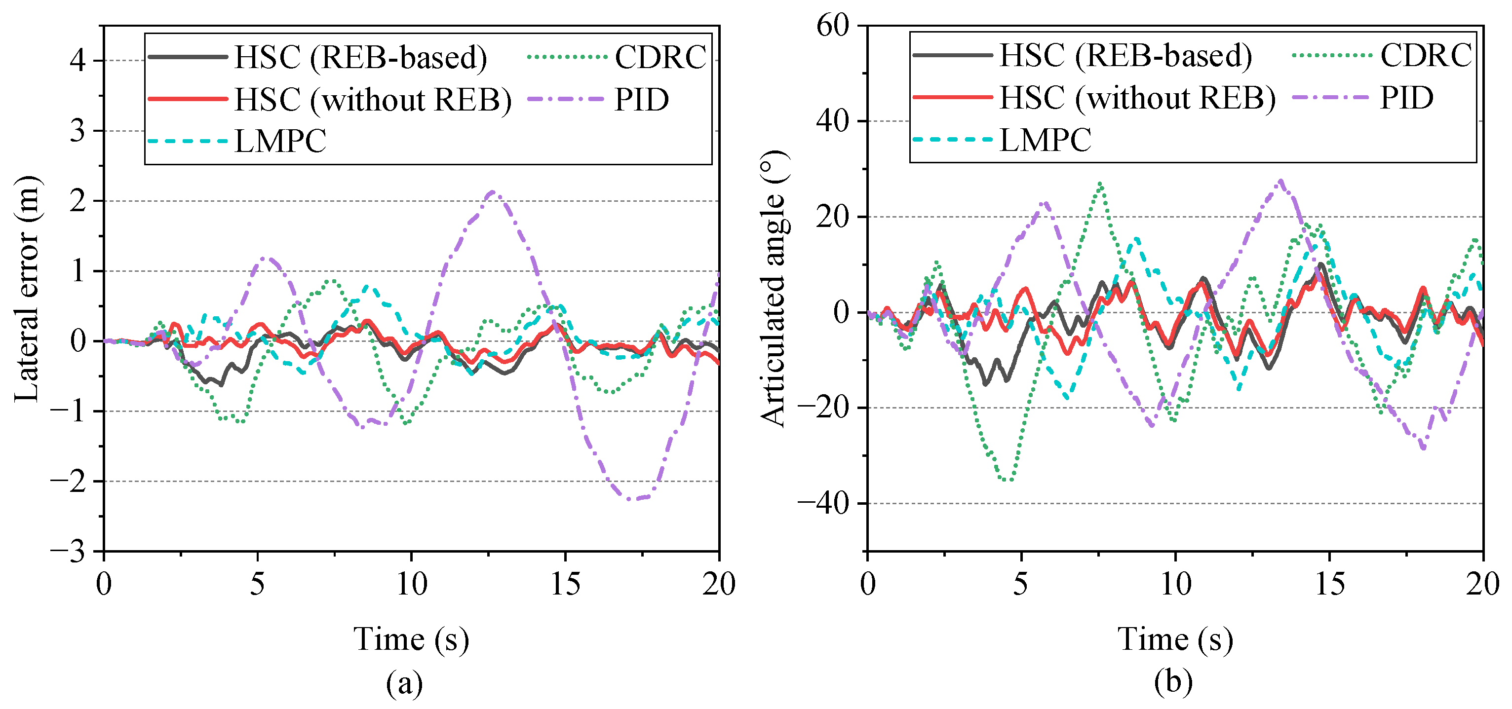
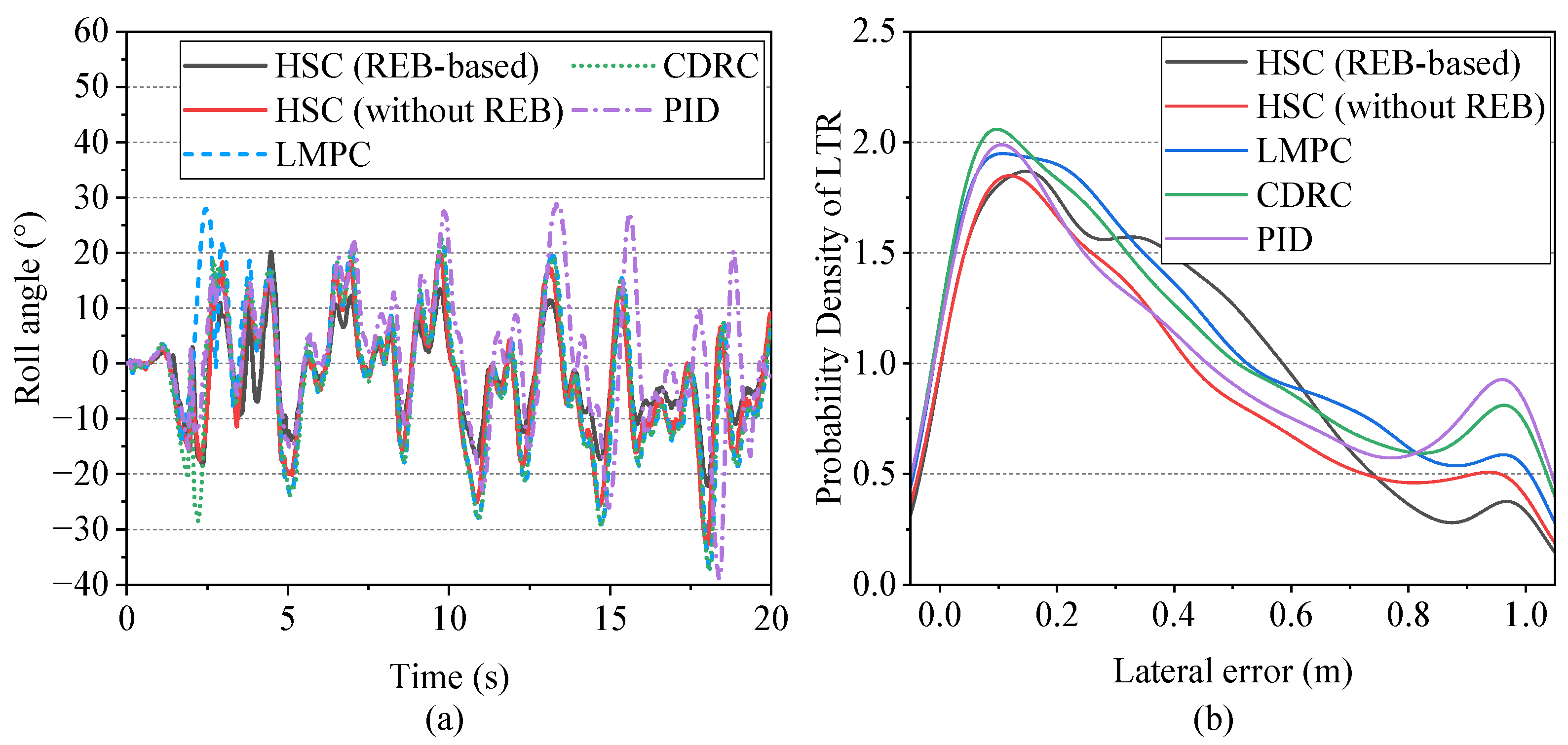
6.2.1. Simulation Experiment

The simulation experiments compare the proposed HSC with single CDRC, LMPC, and PID controllers, focusing on trajectory tracking accuracy, roll stability, and computational efficiency. The PID has already proven its effectiveness in the practice of autonomous driving [46,47], and the LMPC [48], based on a kinematic model, is also widely adopted in autonomous vehicle applications. In addition, a modified HSC, with the weight matrix S in Equation (23) set to zero (i.e., without considering REB), was also included in the experiments. The CDRC, as part of the HSC, can function effectively as an independent controller, demonstrating strong capabilities in disturbance rejection. Building on our previous research [39,40], a CDRC with well-turned ESOs performs well in addressing disturbances such as uneven roads, sensor measurement bias, and ground friction changes, which encompass both slow-varying and rapidly changing disturbances. The parameters of all controllers were optimized using a grid search method. This approach systematically explores the parameter space by testing predefined combinations to identify the set that minimizes key performance metrics, such as overshoot, average error, and maximum REB.

The results of the lateral stability of the UR are illustrated in Figure 13, and the corresponding quantitative indices are summarized in

Table 2. Lateral stability experimental results.

Controllers	Average Lateral Error (m)	Lateral Error Range (m)	Articulated Angle Range (°)	The Standard Deviation of Lateral Error (m)
HSC (REB-based)	0.16	0.90	25.2	0.19
HSC (without REB)	0.11	0.61	17.1	0.13
LMPC	0.23	1.27	34.7	0.27
CDRC	0.43	2.06	62.2	0.52
PID	0.91	4.38	56.0	1.13

. The lateral error over time (Figure 13a) indicates that the proposed HSC (REB-based) demonstrates excellent trajectory tracking performance, with an average lateral error of 0.16 m and a standard deviation of 0.19 m. However, HSC without REB performs even better, with a smaller average lateral error of 0.11 m and a standard deviation of 0.13 m. In contrast, both LMPC and CDRC show moderate performance but exhibit significant oscillatory behavior with lateral error ranges of 1.27 m and 2.06 m, respectively, highlighting their limited robustness in handling bumpy road conditions. The PID controller performs the worst, with its lateral error exceeding ±2 m and standard deviation of 1.13 m, clearly indicating its inability to maintain accurate tracking on uneven terrain.

The articulated angle in Figure 13b also highlights the lateral stability differences between controllers. The two HSCs and LMPC maintain small articulated angle ranges, effectively avoiding excessive oscillations. In contrast, PID and CDRC exhibit articulated angle ranges of 62.2° and 56.0°, respectively. Notably, the oscillations of CDRC are damping and convergent, whereas those of PID are divergent.

With regard to the roll stability, due to the approximate performance of the front and rear body, the discussion primarily focuses on the front body. Figure 14 illustrates the roll angle and LTR, highlighting the superior roll stability of HSC (REB-based) compared to other controllers. The corresponding quantitative data is provided in

Table 3. Roll stability experimental results.

Controllers	Roll Angle Range (°)	Instability Proportion (LTR = 1) (%)	Average REB (J)	The Standard Deviation of REB (J)
HSC (REB-based)	42.3	2.5	93,481	12,125
HSC (without REB)	53.2	3.6	72,192	16,286
LMPC	65.2	4.3	66,069	17,627
CDRC	60.1	5.9	61,615	19,094
PID	67.7	6.9	52,275	24,420

. The HSC (REB-based) achieves the smallest roll angle range of 42.3°, the lowest instability proportion (i.e., the proportion of LTR = 1) at 2.5%, and the highest average REB value of 9.35 × 10⁴ J. In contrast, while the HSC (without REB) demonstrates highest accuracy, it performs worse in roll stability. Specifically, its average REB is 22.7% lower than that of HSC (REB-based), and its instability proportion increases by 44.0%. In addition, the distribution of REB shown in Figure 15 further supports this result. The HSC (REB-based) exhibits the smallest standard deviation of 12,125 J. In contrast, the standard deviations of the other controllers are more than 34.3% higher compared to the HSC (REB-based), reflecting significantly more dispersed distributions and less stable roll energy behavior. This indicates that removing the REB component from the cost function reduces the roll stability of the HSC framework. Furthermore, LMPC, CDRC, and PID exhibit even worse performance than the HSC methods, with larger roll angle ranges and lower average REB values, highlighting a noticeable decline in roll stability compared to HSC (REB-based). Among them, PID performs the worst, with the lowest average REB of 5.23 × 10⁴ J and a minimum REB of only 0.46 × 10⁴ J, severely compromising roll stability.

It is worth noting that the computational real-time performance of the algorithm is a critical factor in practical applications. Leveraging Infineon’s automotive-grade chip platform with a multi-core architecture, we employed parallel computing and code optimization to significantly enhance efficiency. Test results demonstrated that the average computation time of NMPC was reduced to 12.16 ms, while CDRC’s computation time averaged just 0.098 ms. These optimizations ensure stable operation within a 50 ms time slice, achieving a reliable control frequency of 20 Hz.

Overall, the analysis clearly demonstrates the advantages of the HSC (REB-based) in maintaining superior roll stability, followed by the HSC (without REB). The remaining controllers, particularly PID, exhibit significant limitations in handling dynamic rollover conditions.

Considering lateral tracking accuracy, articulated angle stability, and roll stability, the proposed HSC (REB-based) clearly outperforms all the other control methods. The comparison between HSC (REB-based) and HSC (No REB) confirms that incorporating REB into the control framework significantly enhances vehicle performance under bumpy conditions. LMPC and CDRC provide reasonable performance but suffer from higher oscillations and reduced stability, particularly in roll and articulated angle control. PID, while computationally efficient, exhibits the poorest performance across all indices, failing to maintain either trajectory accuracy or stability under challenging conditions.

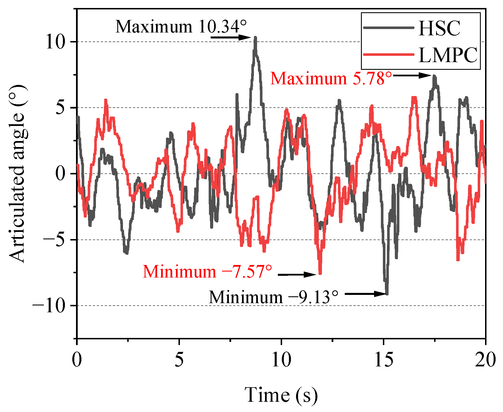
6.2.2. Real UR Experiment

To further validate the effectiveness of the proposed HSC framework compared to LMPC, a real UR experiment was conducted on a bumpy road scenario, as shown in Figure 12b. A protruding rock was intentionally placed in the middle of the path to simulate severe terrain disturbances. The objective was to evaluate the lateral stability and rollover stability of the controllers under dynamic and unpredictable conditions. Figure 16 illustrates the lateral error and roll angle responses for HSC and LMPC, respectively, while Figure 17 and Figure 18 compare the articulated angle and REB, respectively.

As shown in Figure 16, after encountering the protruding rock, HSC initially exhibits a larger lateral error of −0.65 m compared to LMPC. This is due to the sudden disturbance and active steering adjustments, which prioritize roll stability over immediate trajectory accuracy. This prioritization is further evidenced by Figure 17, which indicates that the maximum articulated angle of HSC in the protruding area is 10.34°, larger than that of LMPC. This trade-off allows HSC to rapidly stabilize the lateral error after the initial adjustment phase while simultaneously enhancing roll stability. As shown in Figure 18, HSC reaches the minimum REB 0.12 s earlier than LMPC, and its minimum REB is increased by 57.8%.

HSC emphasizes stability by prioritizing faster recovery from rollover risk and overall system robustness, even at the expense of temporary trajectory accuracy. This is demonstrated by its coordinated steering adjustments, effectively countering destabilizing factors such as protruding rocks. In contrast, LMPC’s rigidity in maintaining accuracy hinders its ability to stabilize quickly, increasing rollover risks during sudden disturbances.

7. Conclusions

This study presents a comprehensive approach to improving rollover stability and trajectory tracking control for URs by introducing the symmetry-inspired REB index and the HSC strategy. The REB index provides a reliable and accurate assessment of rollover risk by quantifying the dynamic balance between the current state and the rollover threshold, while HSC leverages this index to achieve enhanced stability under dynamic conditions.

The REB index demonstrates significant advantages over traditional metrics, including a 32.3% increase in rollover prediction lead time. Additionally, REB shows a notable improvement in handling common challenges such as false positives and missed detections in tripped rollover scenarios. By reflecting the system’s dynamic symmetry and its tendency toward instability, REB provides a sensitive and reliable foundation for precise and consistent control strategies.

Building on the REB index, the HSC control strategy effectively balances lateral and roll stability, showcasing its ability to manage dynamic asymmetries introduced by articulated vehicle dynamics and uneven terrain. Across multiple experiments, HSC maintains trajectory tracking accuracy comparable to other advanced algorithms while achieving a substantial improvement in rollover stability, with an average REB increase of 35.6%. These results underscore HSC’s capability to restore and maintain dynamic symmetry, ensuring faster recovery and enhanced robustness under challenging off-road conditions.

In summary, the combination of REB and HSC offers a superior balance between stability and trajectory-tracking performance, providing a symmetry-inspired framework for improving the safety and robustness of URs. However, challenges remain, particularly in scenarios where uneven ground and side-slip coexist, as well as in cases involving abrupt changes in ground parameters such as tire–road friction coefficients. To address these challenges, future work will focus on enhancing the system’s adaptability to more complex and dynamic road conditions. This may involve integrating HSC with more advanced sensors and improving its control performance under such conditions, ensuring the system can effectively handle a wider range of real-world environments.

References

1. Yang, M.; Bian, Y.; Liu, G.; Zhang, H. Path Tracking Control of an Articulated Road Roller with Sideslip Compensation. IEEE Access 2020, 8, 127981–127992. [Google Scholar] [CrossRef]
2. Yu, S.; Hirche, M.; Huang, Y.; Chen, H.; Allgöwer, F. Model predictive control for autonomous ground vehicles: A review. Auton. Intell. Syst. 2021, 1, 4. [Google Scholar] [CrossRef]
3. Zhang, C.; Wu, J.; Li, C. Recent Progress in Robot Control Systems: Theory and Applications. Symmetry 2024, 16, 43. [Google Scholar] [CrossRef]
4. Carabin, G.; Gasparetto, A.; Mazzetto, F.; Vidoni, R. Design, implementation and validation of a stability model for articulated autonomous robotic systems. Robot. Auton. Syst. 2016, 83, 158–168. [Google Scholar] [CrossRef]
5. Reński, A. Investigation of the Influence of the Centre of Gravity Position on the Course of Vehicle Rollover. In Proceedings of the 24th International Technical Conference on the Enhanced Safety of Vehicles (ESV) National Highway Traffic Safety Administration, Gothenburg, Sweden, 8–11 June 2015. [Google Scholar]
6. Gao, Y.; Shen, Y.; Xu, T.; Zhang, W.; Guvenc, L. Oscillatory Yaw Motion Control for Hydraulic Power Steering Articulated Vehicles Considering the Influence of Varying Bulk Modulus. IEEE Trans. Control Syst. Technol. 2019, 27, 1284–1292. [Google Scholar] [CrossRef]
7. Rowduru, S.; Kumar, N.; Kumar, A. A critical review on automation of steering mechanism of load haul dump machine. Proc. Inst. Mech. Eng. Part I J. Syst. Control Eng. 2019, 234, 160–182. [Google Scholar] [CrossRef]
8. Jin, Z.; Li, B.; Li, J. Dynamic Stability and Control of Tripped and Untripped Vehicle Rollover; Morgan & Claypool Publishers: San Rafael, CA, USA, 2019. [Google Scholar]
9. Phanomchoeng, G.; Rajamani, R. New Rollover Index for the Detection of Tripped and Untripped Rollovers. IEEE Trans. Ind. Electron. 2013, 60, 4726–4736. [Google Scholar] [CrossRef]
10. Tota, A.; Dimauro, L.; Velardocchia, F.; Paciullo, G.; Velardocchia, M. An intelligent predictive algorithm for the anti-rollover prevention of heavy vehicles for off-road applications. Machines 2022, 10, 835. [Google Scholar] [CrossRef]
11. Committee, S.V.D.S. Steady-state directional control test procedures for passenger cars and light trucks. SAE Stand. J. 1996, 266. [Google Scholar]
12. Rakheja, S.; Piche, A. Development of directional stability criteria for an early warning safety device. SAE Trans. 1990, 877–889. [Google Scholar]
13. Gauchía, A.; Olmeda, E.; Aparicio, F.; Díaz, V. Bus mathematical model of acceleration threshold limit estimation in lateral rollover test. Veh. Syst. Dyn. 2011, 49, 1695–1707. [Google Scholar] [CrossRef]
14. Hac, A.; Brown, T.; Martens, J. Detection of Vehicle Rollover; 2004-01-1757; SAE Technical Paper; SAE: Warrendale, PA, USA, 2004. [Google Scholar] [CrossRef]
15. Liu, P.; Rakheja, S.; Ahmed, A. Detection of dynamic roll instability of heavy vehicles for open-loop rollover control. SAE Trans. 1997, 632–639. [Google Scholar]
16. Xu, X.; Ai, X.; Chen, R.; Jiang, G.; Hua, X. Research on roll stability of articulated engineering vehicles based on dynamic lateral transfer load. Proc. Inst. Mech. Eng. Part D J. Automob. Eng. 2020, 234, 2364–2376. [Google Scholar] [CrossRef]
17. Ye, Z.; Xie, W.; Yin, Y.; Fu, Z. Dynamic rollover prediction of heavy vehicles considering critical frequency. Automot. Innov. 2020, 3, 158–168. [Google Scholar] [CrossRef]
18. Zheng, L.; Lu, Y.; Li, H.; Zhang, J. Anti-Rollover Control and HIL Verification for an Independently Driven Heavy Vehicle Based on Improved LTR. Machines 2023, 11, 117. [Google Scholar] [CrossRef]
19. Yang, X.; Wu, C.; He, Y.; Lu, X.-Y.; Chen, T. A dynamic rollover prediction index of heavy-duty vehicles with a real-time parameter estimation algorithm using NLMS method. IEEE Trans. Veh. Technol. 2022, 71, 2734–2748. [Google Scholar] [CrossRef]
20. Jeong, Y. Integrated Vehicle Controller for Path Tracking with Rollover Prevention of Autonomous Articulated Electric Vehicle Based on Model Predictive Control. Actuators 2023, 12, 41. [Google Scholar] [CrossRef]
21. Xia, G.; Li, J.; Tang, X.; Zhang, Y.; Zhao, L. Anti-Rollover of the Counterbalanced Forklift Truck Based on Zero-Moment Point; 0148-7191; SAE Technical Paper; SAE: Warrendale, PA, USA, 2021. [Google Scholar]
22. Hong, H.; Wang, K.; d’Apolito, L.; Quan, K.; Yao, X. Anti-Rollover Control for All-Terrain Vehicle Based on Zero-Moment Point; 0148-7191; SAE Technical Paper; SAE: Warrendale, PA, USA, 2024. [Google Scholar]
23. Wang, H.; Hou, L.; Shangguan, W.-B. Research on vehicle rollover warning and braking control system based on secondary predictive zero-moment point position. SAE Int. J. Adv. Curr. Pract. Mobil. 2022, 4, 1689–1703. [Google Scholar] [CrossRef]
24. Chao, P.-P.; Zhang, R.-Y.; Wang, Y.-D.; Tang, H.; Dai, H.-L. Warning model of new energy vehicle under improving time-to-rollover with neural network. Meas. Control 2022, 55, 1004–1015. [Google Scholar] [CrossRef]
25. Chen, X.; Chen, W.; Hou, L.; Hu, H.; Bu, X.; Zhu, Q. A novel data-driven rollover risk assessment for articulated steering vehicles using RNN. J. Mech. Sci. Technol. 2020, 34, 2161–2170. [Google Scholar] [CrossRef]
26. Zhu, T.; Yin, X.; Na, X.; Li, B. Research on a Novel Vehicle Rollover Risk Warning Algorithm Based on Support Vector Machine Model. IEEE Access 2020, 8, 108324–108334. [Google Scholar] [CrossRef]
27. Zhu, T.; Yin, X.; Li, B.; Ma, W. A Reliability Approach to Development of Rollover Prediction for Heavy Vehicles Based on SVM Empirical Model with Multiple Observed Variables. IEEE Access 2020, 8, 89367–89380. [Google Scholar] [CrossRef]
28. Mao, Y.; Wu, Y.; Yan, X.; Liu, M.; Xu, L. Simulation and experimental research of electric tractor drive system based on Modelica. PLoS ONE 2022, 17, e0276231. [Google Scholar] [CrossRef] [PubMed]
29. Ensbury, T.; Horn, N.; Dempsey, M. Dymola and Simulink in Co-Simulation: A Vehicle Electronic Stability Control Case Study. 2020. Available online: https://www.claytex.com/wp-content/uploads/2021/06/Dymola-and-Simulink-in-Co-Simulation_-a-case-study.pdf (accessed on 2 January 2025).
30. Bhoraskar, A.; Sakthivel, P. A review and a comparison of Dugoff and modified Dugoff formula with Magic formula. In Proceedings of the 2017 International Conference on Nascent Technologies in Engineering (ICNTE), Vashi, Navi Mumbai, India, 27–28 January 2017; pp. 1–4. [Google Scholar]
31. Pacejka, H.B.; Bakker, E. The magic formula tyre model. Veh. Syst. Dyn. 1992, 21, 1–18. [Google Scholar] [CrossRef]
32. Vafaei, N.; Fakharian, K.; Sadrekarimi, A. Sand-sand and sand-steel interface grain-scale behavior under shearing. Transp. Geotech. 2021, 30, 100636. [Google Scholar] [CrossRef]
33. Ziogos, A.; Brown, M.J.; Ivanovic, A.; Morgan, N. Understanding rock–steel interface properties for use in offshore applications. Proc. Inst. Civ. Eng.-Geotech. Eng. 2023, 176, 27–41. [Google Scholar] [CrossRef]
34. Zhou, W.; Guo, Z.; Wang, L.; Li, J.; Rui, S. Sand-steel interface behaviour under large-displacement and cyclic shear. Soil Dyn. Earthq. Eng. 2020, 138, 106352. [Google Scholar] [CrossRef]
35. Rui, S.; Wang, L.; Guo, Z.; Cheng, X.; Wu, B. Monotonic behavior of interface shear between carbonate sands and steel. Acta Geotech. 2021, 16, 167–187. [Google Scholar] [CrossRef]
36. Aksoy, H.S.; Taher, N.R.; Ozpolat, A.; Gör, M.; Edan, O.M. An Experimental Study on Estimation of the Lateral Earth Pressure Coefficient (K) from Shaft Friction Resistance of Model Piles under Axial Load. Appl. Sci. 2023, 13, 9355. [Google Scholar] [CrossRef]
37. Mei, Z.; Xiao, A.; Mei, J.; Hu, J.; Zhang, P. Experimental Study on Interface Frictional Characteristics between Sand and Steel Pipe Jacking. Appl. Sci. 2023, 13, 2016. [Google Scholar] [CrossRef]
38. Jin, X.; Li, Z.; Opinat Ikiela, N.V.; He, X.; Wang, Z.; Tao, Y.; Lv, H. An Efficient Trajectory Planning Approach for Autonomous Ground Vehicles Using Improved Artificial Potential Field. Symmetry 2024, 16, 106. [Google Scholar] [CrossRef]
39. Quanzhi, X.; Hui, X.; Kang, S. The Impact of Control Structure on the Path-Following Control of Unmanned Compaction Rollers. In Proceedings of the SAE 2019 Intelligent and Connected Vehicles Symposium, Shanghai, China, 22–23 September 2020. [Google Scholar]
40. Xie, H.; Xu, Q.; Song, K. Layered disturbance rejection path-following control with geometry-based feedforward for unmanned rollers. Proc. Inst. Mech. Eng. Part D J. Automob. Eng. 2023, 237, 1435–1453. [Google Scholar] [CrossRef]
41. Jin, X.; Lv, H.; He, Z.; Li, Z.; Wang, Z.; Ikiela, N.V.O. Design of Active Disturbance Rejection Controller for Trajectory-Following of Autonomous Ground Electric Vehicles. Symmetry 2023, 15, 1786. [Google Scholar] [CrossRef]
42. Quirynen, R.; Di Cairano, S. Sequential quadratic programming algorithm for real-time mixed-integer nonlinear MPC. In Proceedings of the 2021 60th IEEE Conference on Decision and Control (CDC), Austin, TX, USA, 13–17 December 2021; pp. 993–999. [Google Scholar]
43. Rajkumar, S. Nonlinear Model Predictive Control: An Implementation Using CasADi; The Ohio State University: Columbus, OH, USA, 2024. [Google Scholar]
44. Sun, N.; Zhang, W.; Yang, J. Integrated Path Tracking Controller of Underground Articulated Vehicle Based on Nonlinear Model Predictive Control. Appl. Sci. 2023, 13, 5340. [Google Scholar] [CrossRef]
45. Jin, Z.; Weng, J.; Hu, H. Rollover stability of a vehicle during critical driving manoeuvres. Proc. Inst. Mech. Eng. Part D J. Automob. Eng. 2007, 221, 1041–1049. [Google Scholar] [CrossRef]
46. Bian, Y.; Yang, M.; Fang, X.; Wang, X. Kinematics and path following control of an articulated drum roller. Chin. J. Mech. Eng. 2017, 30, 888–899. [Google Scholar] [CrossRef]
47. Zhang, Z.; Fang, M.; Fei, M.; Li, J. Robust and Exponential Stabilization of a Cart–Pendulum System via Geometric PID Control. Symmetry 2024, 16, 94. [Google Scholar] [CrossRef]
48. Zhang, K.; Wang, J.; Xin, X.; Li, X.; Sun, C.; Huang, J.; Kong, W. A Survey on Learning-Based Model Predictive Control: Toward Path Tracking Control of Mobile Platforms. Appl. Sci. 2022, 12, 1995. [Google Scholar] [CrossRef]
Figure 1. The structure of the single-drum articulated roller.
Symmetry 17 00118 g001
Figure 2. The single-drum articulated roller in this research.
Symmetry 17 00118 g002
Figure 3. The dynamic model of the UR: (a) the front body roll dynamic; (b) the rear body roll dynamic; (c) the UR’s horizontal dynamic.
Symmetry 17 00118 g003
Figure 4. The tire and front drum model of the UR: (a) The rear tire model; (b) The front drum model.
Symmetry 17 00118 g004
Figure 5. The structure of the hydraulic steering system: (1) Hydraulic pump; (2) Relief valves; (3) Hydraulic oil tank; (4) 3-position, 4-way directional control valve; (5) Check valves; (6) Double-acting cylinders.
Symmetry 17 00118 g005
Figure 6. The diagram of rollover energy: (a) The critical rollover state; (b) The general roll state; (c) The equivalence of the general roll state.
Symmetry 17 00118 g006
Figure 7. The controller diagram of HSC.
Symmetry 17 00118 g007
Figure 8. The trajectories of the untripped rollover experiments.
Symmetry 17 00118 g008
Figure 9. Untripped rollover experimental results: (a) Lateral acceleration; (b) LTR; (c) REB.
Symmetry 17 00118 g009
Figure 10. Tripped rollover simulation experimental scenario.
Symmetry 17 00118 g010
Figure 11. Tripped rollover experimental results: (a) Lateral acceleration; (b) LTR; (c) REB.
Symmetry 17 00118 g011
Figure 12. Uneven terrain experimental scenarios: (a) Simulation scenario; (b) Real-world scenario.
Symmetry 17 00118 g012
Figure 13. Lateral stability experimental results: (a) Lateral error; (b) Articulated angle.
Symmetry 17 00118 g013
Figure 14. Roll stability experimental results: (a) Front roll angle; (b) LTR distribution.
Symmetry 17 00118 g014
Figure 15. The distribution of REB.
Symmetry 17 00118 g015
Figure 16. The real UR experimental results: (a) HSC; (b) LMPC.
Symmetry 17 00118 g016
Figure 17. The articulated angle results on uneven terrain.
Symmetry 17 00118 g017
Figure 18. The REB results on uneven terrain.
Symmetry 17 00118 g018