SDA-RRT*Connect: A Path Planning and Trajectory Optimization Method for Robotic Manipulators in Industrial Scenes with Frame Obstacles

Abstract

The trajectory planning of manipulators plays a crucial role in industrial applications. This importance is particularly pronounced when manipulators operate in environments filled with obstacles, where devising paths to navigate around obstacles becomes a pressing concern. This study focuses on the environment of frame obstacles in industrial scenes. At present, many obstacle avoidance trajectory planning algorithms struggle to strike a balance among trajectory length, generation time, and algorithm complexity. This study aims to generate path points for manipulators in an environment with obstacles, and the trajectory for these manipulators is planned. The search direction adaptive RRT*Connect (SDA-RRT*Connect) method is proposed to address this problem, which adaptively adjusts the search direction during the search process of RRT*Connect. In addition, we design a path process method to reduce the length of the path and increase its smoothness. As shown in experiments, the proposed method shows improved performances with respect to path length, algorithm complexity, and generation time, compared to traditional path planning methods. On average, the configuration space’s path length and the time of generation are reduced by 38.7% and 57.4%, respectively. Furthermore, the polynomial curve trajectory of the manipulator was planned via a PSO algorithm, which optimized the running time of the manipulator. According to the experimental results, the proposed method costs less time during the manipulator’s traveling process with respect to other comparative methods. The average reduction in running time is 45.2%.

1. Introduction

Robotic manipulators have assumed a more significant role in industrial fields, including manufacturing [1], logistics [2], warehousing [3], and aerospace [4]. Manipulators can fulfill diverse tasks and operations across these fields. Whether it pertains to manufacturing for machining, logistics for handling, or aerospace for attitude control, each field necessitates the meticulous refinement of motion paths for manipulators and the precise planning of end effector trajectories. In real industrial applications, obstacles are often extremely complex. Considering the pertinence of the research, we only focus on frame obstacles in industrial scenes. In the environment with frame obstacles, obstacle avoidance is an indispensable component in path planning for manipulators. Hence, research on obstacle avoidance trajectory planning for manipulators stands as one of the most critical aspects within the field of manipulator studies.

Traditional path planning algorithms include the Dijkstra algorithm [5]; A* algorithm [6]; artificial potential field (APF) method [7]; and heuristic optimization algorithms [8], such as the particle swarm optimization (PSO) algorithm [9] and genetic algorithm (GA) [10]. However, when applied to manipulators, these algorithms often fall short in achieving optimal results in terms of path generation efficiency and path quality.

Global obstacle avoidance path planning for a manipulator refers to the process of determining feasible paths in a known environment with predefined obstacle positions and shapes. In the domain of global obstacle avoidance trajectory planning for manipulators in a configuration space, sampling-based methods have frequently been employed to plan path points for manipulators. The most common sampling-based path planning algorithms include the probabilistic roadmap (PRM) algorithm [11] and rapidly exploring random tree (RRT) algorithm [12]. Many researchers favor the RRT algorithm due to its simple structure and strong adaptability. Thus far, several improvement methods for RRT have been widely adopted by researchers, such as RRT* [13], RRT-Connect [14], RRT* Connect [15], and RRT*Smart [16].

Path generation time, trajectory running time, and path length are significant evaluation indicators in the field of trajectory planning. Path generation time indicates the efficiency of the algorithm in generating path points. Trajectory running time directly determines the efficiency of the robotic arm in completing the task. Moreover, the length of the path includes lengths in the configuration space and workspace. The former represents the amount of the change joint’s angle. It can further characterize the energy consumption of the robotic arm. The latter represents the length and smoothness of the motion trajectory of the end of the robotic manipulator in the real world. Despite the advancements achieved in their respective domains via improvements to the RRT algorithm, most current enhanced RRT algorithms fail to comprehensively optimize the three above-mentioned indicators. This is because these algorithms do not combine the configuration space of the manipulator with the workspace and cannot highlight the pertinence of the algorithm for the robotic arm. Therefore, there is still room for improvement in applying this algorithm in the field of robotic manipulator trajectory planning. The contributions of this article are outlined below.

(1) The proposed improved algorithm, search direction adaptive RRT*Connect (SDA-RRT*Connect), which is based on the RRT algorithm, is introduced. It can adaptively and rationally adjust the search direction to alter the search process at different stages of the algorithm, enabling it to find feasible paths rapidly.

(2) A novel method for handling path points is proposed to address issues such as path crossing and oscillations in the workspace. This method enhances path smoothness and reduces path length in the workspace.

(3) The PSO algorithm is used to fit polynomial curves for each segment of the path, aiming to minimize the trajectory execution time of the manipulator under velocity and acceleration constraints.

(4) Comparative simulation experiments are conducted to validate that the proposed method achieves superior results in terms of path generation time, trajectory execution time, and path length.

2. Related Works

Regarding further improved algorithms of RRT in the field of manipulator trajectory planning, researchers have carried out numerous attempts. Among these, many methods were proposed to enhance the algorithms by optimizing the structure of the exploration tree. Wu et al. [17] proposed an obstacle avoidance path planning algorithm based on the central multi-node RRT* (CMN-RRT) algorithm. This study primarily focused on addressing the challenges of lengthy computation times and inadequate obstacle avoidance effectiveness in traditional RRT algorithms. The primary enhancement focuses on optimizing the sampling strategy of the traditional algorithm. The concept of connectivity was introduced during the path’s growth process, allowing multiple trees to grow simultaneously and thereby facilitating quicker obstacle avoidance. Song et al. [18] proposed an enhanced RRT algorithm based on the probability target deviation strategy and the triangle inequality pruning method in order to tackle lengthy computation times and the generation of lengthy paths in motion planning for manipulators using the RRT algorithm.

In addition to optimizing the tree structure, improving the sampling process can also effectively enhance the performance of the algorithm. Shen et al. [19] proposed a new optimal RRT path planning strategy based on operability for industrial manipulators. Two constraints, namely path length and the operability measure, were imposed during sampling in the search space to find the minimum-cost path connecting the start and goal points. By tracing the generated paths, the manipulator’s end effector could navigate the workspace with shorter distances. Wang et al. [20] proposed a method for setting the intermediate bias point. In random sampling, the sampling point was biased towards the intermediate bias point with a certain probability in order to reduce the blindness of sampling. Thakar et al. [21] introduced a bi-directional sampling-based approach for generating robotic trajectories for pick-and-place tasks along a given mobile base trajectory. The method implicitly determined the positions of the mobile base at the beginning and end of the robot’s motion, as well as the location where grasping occurs. It also identified the grasp poses used for picking up parts. Additionally, techniques for reducing robot motion and computation times were proposed. Du et al. [22] proposed an improvement to the RRT algorithm by introducing a node attractive field function, which can reduce the generation of redundant nodes, thereby enhancing the convergence speed of the path. Yi et al. [23] presented an enhanced approach for robotic path planning using the improved P_RRT* algorithm to address path planning challenges in workspace for manipulators. Jiang et al. [24] developed a collision detection model for manipulators and obstacles based on cylindrical and spherical bounding boxes. They replaced random sampling with hybrid constraint sampling and introduced a new method called RRT-Connect by combining artificial potential field techniques. Ji et al. [25] proposed an ellipsoidal rapidly exploring random tree (E-RRT*) method for the path planning of highly redundant manipulators (HRM) in work spaces.

Additionally, researchers also enhanced the algorithm to operate effectively in dynamic environments. Qi et al. [26] proposed the MOD-RRT* algorithm, which generates an initial path and constructs a state tree structure based on a known map. They introduced a path replanning scheme to navigate around unknown obstacles and proposed a path smoothing method. In addition, they designed a reconnection scheme to optimize tree structures in the presence of unknown obstacles. Moreover, they presented a multi-objective path replanning method based on Pareto theory to select the optimal alternative nodes when obstacles obstruct pre-planned paths. Zhao et al. [27] proposed the dynamic RRT algorithm. The objective was to devise feasible paths in environments with randomly distributed obstacles while balancing convergence time and path length. Furthermore, by embracing dynamic programming principles, they decomposed the planning problem into sub-problems by updating nodes selected through Pareto dominance as new starting nodes, thereby optimizing the distance to the goal. Zhou et al. [28] proposed the RRT*-FDWA algorithm for dynamic environments—this algorithm can avoid local minima, quickly perform path replanning, generate smooth optimal paths, and increase the robot’s maneuvering range. Yuan et al. [29] proposed a multi-query and sampling motion replanning algorithm named DBG-RRT based on a dynamic deviation goal factor for the obstacle avoidance problem of robotic arms in dynamic environments in order to achieve rapid responses and a high success rate. This method uses a relay node approach to generate new collision-free trajectories on the basis of motion planning. Subsequently, a non-interruption strategy is adopted to determine whether dynamic obstacles will interfere with the generated trajectories.

Integrating the RRT algorithm with optimization problems can also enhance the effectiveness of the algorithm. Khan et al. [30] utilized the intelligent weighted Jacobian rapidly exploring random tree (WJRRT) algorithm to propose a model-free control framework for the path planning of both rigid and flexible manipulators. This framework addressed uncertainties in manipulators and enhanced the computational efficiency of path planning. Gao et al. [31] proposed a path planning method for six-degree-of-freedom robotic manipulators in narrow spaces with multiple obstacles in 3D. They addressed issues such as slow-motion planning, low efficiency, and high path computation costs. Their method—named BP-RRT* and based on a BP neural network and an improved rapidly exploring random trees algorithm—aimed to overcome these challenges and enhance the efficiency of robotic manipulator path planning. Shi et al. [32] introduced the GA_RRT path planning algorithm by incorporating the target probability bias strategy and an A* cost function into the traditional RRT algorithm. This approach reduced the randomness and blindness during the expansion process of the RRT algorithm. Long et al. [33] introduced a novel motion planner called RRT*Smart-AD. It was designed to ensure that dual-arm robots adhere to obstacle avoidance constraints and dynamic characteristics within dynamic environments.

The above are the improvements made by researchers to RRT from different aspects for this task in recent years.

3. Problem Statement

In this section, the definition of the path planning problem for a manipulator is provided, and the mathematical notation involved in the subsequent sections is elucidated. $CS\subseteq {\mathbb{R}}^N$ denotes the configuration space of the manipulator, where N is the degrees of freedom of the manipulator. Generally speaking, the value of N is equal to the number of axes included in the robotic arm. $RS\subseteq CS$ is the reachable space. It includes all the states that the manipulator can reach. $WS\subseteq {\mathbb{R}}^3$ is the workspace of the manipulator. It denotes the set of points where the end of manipulator can reach. Forward kinematic mapping is $F_{\mathrm{fk}}:RS\to WS$, which maps the reachable space to the workspace. The starting point and end point are, respectively, $q_{\mathrm{init}}$ and $q_{\mathrm{goal}}$. The information of obstacles in the environment is O. In this problem, obstacles are stationary. Moreover, the positions of obstacles included in O are given.

We need to plan a trajectory $T=(\tau ,p)$ from $q_{\mathrm{init}}$ to $q_{\mathrm{goal}}$. Here, $\tau =[{\tau }_1,{\tau }_1,\cdots ,{\tau }_{(m-1)n}]$$\in {\mathbb{R}}^{(m-1)n}$ is a time series. $\tau$ increases from zero. m, n, and p are the number of path points, number of moments between different path points, and information on manipulators during all moments, respectively. $p=[p_1,p_2,\cdots ,p_{(m-1)n}]$, $p_i\in RS,i=1,2,\cdots ,(m-1)n$, where $p_i=q_{\mathrm{init}}$ and $p_{(m-1)n}=q_{\mathrm{goal}}$.

The entire process is divided into two steps, as illustrated in Figure 1. Firstly, the path planning algorithm in the configuration space of the manipulator $F_p$ is used to plan a series of path points in the trajectory $C=[c_1,c_2,\cdots ,c_m]$ to avoid obstacles in the environment, where $c_i\in RS,i=1,2,\cdots ,m$, and m denotes the number of path points. This process corresponds to the first stage in Figure 1, which is called path points generation.

$$C=F_p(F_{\mathrm{fk}},q_{\mathrm{init}},q_{\mathrm{goal}},O)$$

(1)

Subsequently, based on the aforementioned path points, an optimization algorithm is employed to fit trajectory curves to minimize the optimization target. A polynomial curve is fitted between each pair of path points as the trajectory curve of the manipulator in this section. The trajectory optimization of the curve is conducted based on the manipulator’s operating time. This process corresponds to the second stage in Figure 1, which is called trajectory optimization. The optimization problem is described below:

$$\begin{array}{c}\hfill min{t}_{i,n}-t_{i,1}\end{array}$$

(2a)

$$\begin{array}{cc}\hfill \mathrm{s}.\mathrm{t}.& q_{i,j}=F_{q,i}\left(t_{i,j}\right),j=1,2,\cdots ,n\hfill \end{array}$$

(2b)

$$\begin{array}{cc}& V_{i,j}\le V_{\max },j=1,2,\cdots ,n\hfill \end{array}$$

(2c)

$$\begin{array}{cc}& A_{i,j}\le A_{\max },j=1,2,\cdots ,n\hfill \end{array}$$

(2d)

$$\begin{array}{cc}& {\Theta }_i=\tilde{\Theta }\hfill \end{array}$$

(2e)

In the above formula, $t_{i,j}$ is the running time in moment j of the manipulator in the ith trajectory. $q_{i,j}$ is the joint angle of manipulator in this trajectory. $F_{q,i}$ is the polynomial function corresponding to this curve. $V_{i,j}$, $A_{i,j}$, and $q_{i,j}$ are velocity, acceleration, and joint angle of moment j in this trajectory fragment, respectively. $\Theta ={[q_{i,0}^{\mathrm{T}},V_{i,0}^{\mathrm{T}},A_{i,0}^{\mathrm{T}},q_{i,n}^{\mathrm{T}},V_{i,n}^{\mathrm{T}},A_{i,n}^{\mathrm{T}}]}^{\mathrm{T}}$, $\tilde{\Theta }={[{\theta }_{i,0}^{\mathrm{T}},v_{i,0}^{\mathrm{T}},a_{i,0}^{\mathrm{T}},{\theta }_{i,g}^{\mathrm{T}},v_{i,g}^{\mathrm{T}},a_{i,g}^{\mathrm{T}}]}^{\mathrm{T}}$, ${\theta }_{i,0}$, ${\theta }_{i,g},v_{i,0},v_{i,g},a_{i,0},a_{i,g}$ are initial angle, termination angle, initial velocity, termination velocity, initial acceleration, and termination acceleration, respectively.

According to the properties of a polynomial curve, the set of manipulator state values corresponding to the ith curve is as follows:

$$p_i=[p_{(i-1)n+1},p_{(i-1)n+2},\cdots ,p_{(i-1)n+n}]=F_q(\Delta t_i),i=1,2,\cdots ,m-1$$

(3)

with $\Delta t_i=t_{i,n}-t_{i,1}$. $F_q$ is a polynomial function, and its parameters are determined by $\Delta t_i$.

Finally, we can obtain trajectory T by connecting each $p_i$ and $t_i$ vector.

$$\tau =[t_1,t_2,\cdots ,t_{m-1}],p=[p_1,p_2,\cdots ,p_{m-1}]$$

(4)

$$T=(\tau ,p)$$

(5)

The key to addressing the above issues is to design a function $F_q$ to obtain the set of path points. Then, the obstacle avoidance trajectory planning of the manipulator can be achieved. The design of the function $F_q$ will be introduced below.

4. SDA-RRT*Connect Path Planning

For the key function $F_q$ mentioned above, this article presents a path planning method for the manipulator based on the improved RRT algorithm as the implementation of the function.

4.1. RRT*Connect

The RRT algorithm is a sampling-based path planning algorithm. Its basic steps involve generating an exploration tree from the starting point of the path. This is achieved by continuously expanding the tree’s leaf nodes through random node sampling. Ultimately, when a leaf node reaches or comes close to the target point, a feasible path is successfully obtained. By continuously tracing back to its parent nodes from this point, the final planned result can be determined.

The RRT* and RRT-Connect algorithm are both improved versions of the traditional RRT algorithm. Each introduces specific enhancements aimed at improving the path cost and the time needed to generate the path. RRT*Connect combines elements from both the RRT* algorithm and RRT-Connect algorithm.

The RRT*Connect algorithm introduces two primary enhancements over the traditional RRT algorithm. Firstly, it employs the simultaneous expansion of two exploration trees from the start and goal points to search for feasible paths because of the symmetry between start and goal points in the configuration space of the manipulator. Specifically, a separate exploration tree is established at both the start and goal points of the path. Through sampling, both trees are continuously expanded simultaneously. During the expansion of either tree, if a new node reaches or approaches a node in the other tree, a viable path is successfully identified. By backtracking the parent nodes of these two nodes in their respective trees, the final planned path can be determined.

Additionally, RRT*Connect incorporates the optimization of the path length during path expansion. Specifically, this method introduces two new operations during node expansion. Firstly, it entails reselecting the parent node. After generating a new node using the traditional RRT algorithm, it explores neighboring nodes within a certain distance of the new node. If traversing through a neighbor node can result in a shorter path length to reach the new node, that neighbor node is reassigned as the parent node of the new node. Secondly, it involves reconnecting neighboring nodes. After identifying the parent node for the new node, it continues to explore neighboring nodes. If traversing through the new node can result in a shorter path length for reaching a neighboring node, the parent node of that neighboring node is reassigned to be the new node.

4.2. Adaptive Search Direction

Aiming at the environment of frame obstacles in industrial scenes, we propose the SDA-RRT*Connect algorithm. The proposed method proposes an optimization method for the RRT*Connect algorithm based on the search direction. As shown in Algorithm 1, the input of algorithm $M=(RS,O)$ is the environment of the manipulator. $q_{\mathrm{init}}$ is the starting position, and $q_{\mathrm{goal}}$ is the target position. StepSize is the step size for expanding nodes in the exploration tree. R denotes the critical distance of neighboring nodes. The MaxIter is the maximum number of iterations. The output of the algorithm $C=[c_1,c_2,\cdots ,c_m]$ is a path from the starting point to the target point, where $c_i\in RS,i=1,2,\cdots ,m$. $T_{\mathrm{start}}$, and $T_{\mathrm{end}}$ are two exploration trees rooted at the start and goal points.

$$q_{\mathrm{new}}=q_{\mathrm{near}}+\mathrm{StepSize}·\left(\lambda ·{\displaystyle \frac{q_{\mathrm{rand}}-q_{\mathrm{near}}}{\parallel q_{\mathrm{rand}}-q_{\mathrm{near}}\parallel }}+(1-\lambda )·{\displaystyle \frac{q_{\mathrm{attr}}-q_{\mathrm{near}}}{\parallel q_{\mathrm{attr}}-q_{\mathrm{near}}\parallel }}\right)$$

(6)

Algorithm 1 SDA-RRT*Connect

Require:  $M,q_{\mathrm{init}},q_{\mathrm{goal}},\mathrm{StepSize},\mathrm{R},\mathrm{MaxIter}$ Ensure:  path C from $q_{\mathrm{init}}$ to $q_{\mathrm{goal}}$   1: $T_{\mathrm{start}}.\mathrm{init}\left(\right),T_{\mathrm{end}}.\mathrm{init}\left(\right)$   2: for $i=1\to \mathrm{MaxIter}$ do   3:      $q_{\mathrm{rand}}\leftarrow \mathrm{Sample}\left(M\right)$   4:      $q_{\mathrm{near},\mathrm{start}}\leftarrow \mathrm{Near}(q_{\mathrm{rand}},T_{\mathrm{start}})$   5:      $q_{\mathrm{attr}}\leftarrow \mathrm{GetAttr}(q_{\mathrm{near},\mathrm{start}},T_{\mathrm{end}})$   6:      $\mathit{\lambda }\leftarrow \mathbf{GetLambda}({\mathit{T}}_{\mathbf{start}},{\mathit{T}}_{\mathbf{end}})$   7:      ${\mathit{q}}_{\mathbf{new},\mathbf{start}}\leftarrow \mathbf{Steer}({\mathit{q}}_{\mathbf{rand}},{\mathit{q}}_{\mathbf{attr}},{\mathit{q}}_{\mathbf{near},\mathbf{start}},\mathbf{StepSize},\mathit{\lambda })$   8:      $q_{\mathrm{parent}}\leftarrow \mathrm{FindParent}(q_{\mathrm{new},\mathrm{start}},T_{\mathrm{start}},\mathrm{R})$   9:      if $\mathrm{CollisionFree}(M,q_{\mathrm{new},\mathrm{start}},q_{\mathrm{parent}})$ then 10:          $T_{\mathrm{start}}.\mathrm{Add}(q_{\mathrm{new},\mathrm{start}},q_{\mathrm{parent}})$ 11:          $\mathrm{Rewire}(q_{\mathrm{new},\mathrm{start}},T_{\mathrm{start}},\mathrm{R})$ 12:      end if 13:      if $\mathrm{Terminal}(q_{\mathrm{new},\mathrm{start}},T_{\mathrm{end}})$ then 14:          $C\leftarrow \mathrm{GetPath}(q_{\mathrm{new},\mathrm{start}},T_{\mathrm{start}},T_{\mathrm{end}})$ 15:          return C 16:      end if 17:      $q_{\mathrm{near},\mathrm{end}}\leftarrow \mathrm{Near}(q_{\mathrm{rand}},T_{\mathrm{end}})$ 18:      $q_{\mathrm{attr}}\leftarrow \mathrm{GetAttr}(q_{\mathrm{near},\mathrm{end}},T_{\mathrm{start}})$ 19:      ${\mathit{q}}_{\mathbf{new},\mathbf{end}}\leftarrow \mathbf{Steer}({\mathit{q}}_{\mathbf{rand}},{\mathit{q}}_{\mathbf{attr}},{\mathit{q}}_{\mathbf{near},\mathbf{end}},\mathbf{StepSize},\mathit{\lambda })$ 20:      $q_{\mathrm{parent}}\leftarrow \mathrm{FindParent}(q_{\mathrm{new},\mathrm{end}},T_{\mathrm{end}},\mathrm{R})$ 21:      if $\mathrm{CollisionFree}(M,q_{\mathrm{new},\mathrm{end}},q_{\mathrm{parent}})$ then 22:          $T_{\mathrm{end}}.\mathrm{Add}(q_{\mathrm{new},\mathrm{end}},q_{\mathrm{parent}})$ 23:          $\mathrm{Rewire}(q_{\mathrm{new},\mathrm{end}},T_{\mathrm{end}},\mathrm{R})$ 24:      end if 25:      if $\mathrm{Terminal}(q_{\mathrm{new},\mathrm{end}},T_{\mathrm{start}})$ then 26:          $C\leftarrow \mathrm{GetPath}(q_{\mathrm{new},\mathrm{end}},T_{\mathrm{start}},T_{\mathrm{end}})$ 27:          return C 28:      end if 29: end for

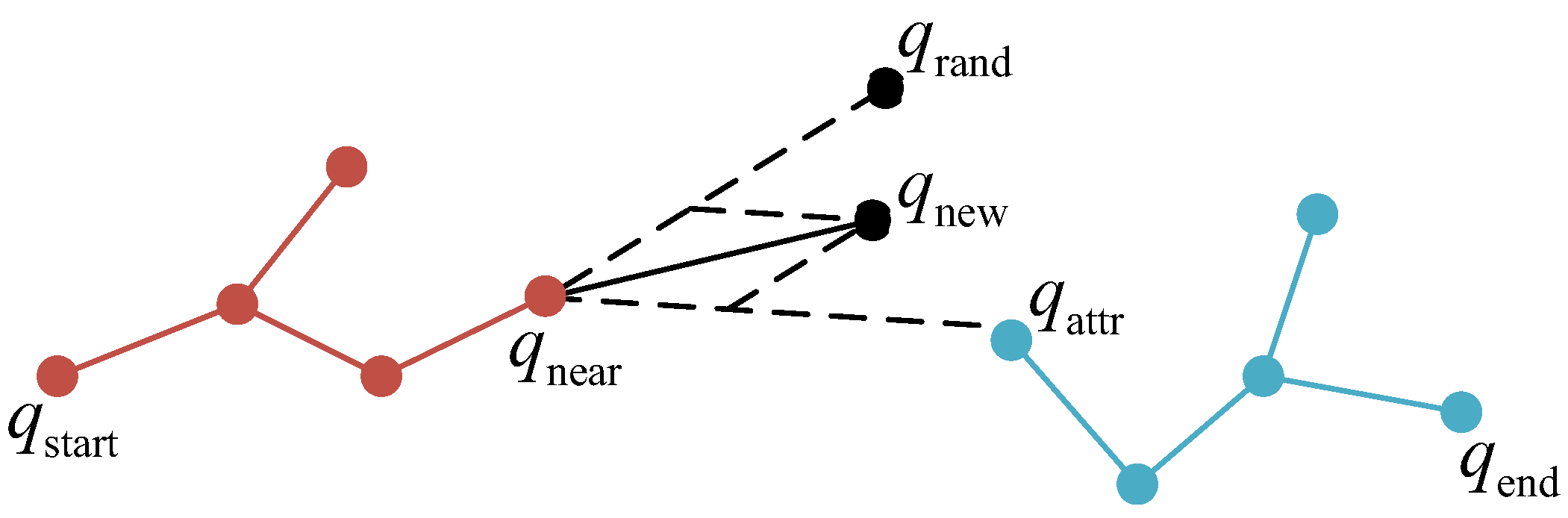
The algorithm operates as follows. First, we obtain $q_{\mathrm{rand}}$ by sampling randomly. Then, we find the node $q_{\mathrm{near},\mathrm{start}}$ in $T_{\mathrm{start}}$, which has the shortest distance with $q_{\mathrm{rand}}$. After that, we should find the node $q_{\mathrm{attr}}$ in $T_{\mathrm{end}}$, which has the shortest distance with $q_{\mathrm{near},\mathrm{start}}$. As shown in Figure 2, vector $(q_{\mathrm{near},\mathrm{start}},q_{\mathrm{rand}})$ implies the direction of random expansion, and vector $(q_{\mathrm{near},\mathrm{start}},q_{\mathrm{attr}})$ implies the direction of targeted expansion. The final direction of expansion will be determined by their sum. We set a parameter $\lambda$ to control the weight of the two directions of expansion. The generation of the new node $q_{\mathrm{new}}$ is shown as (6), and it corresponds to the Steer function in line 7 of Algorithm 1. An increase in $\lambda$ indicates a tendency towards more random expansion, and a decrease in $\lambda$ denotes a tendency towards the other tree. When we obtain the new node, as the RRT*Connect does, we need to choose the father node for the new node. Then, collision detection is performed on the newly generated nodes and edges. If there is no collision, the neighboring nodes of the new node are reconnected according to the rules of the RRT*Connect algorithm. If the new node satisfies the termination condition of the algorithm, the algorithm ends and returns the path. If it does not satisfy the condition, the same process is carried out on $T_{\mathrm{end}}$ because of the symmetry between start and goal points. The above steps are repeated until the two trees are connected.

Due to the diverse requirements for expansion directions during different stages of the algorithm process, the concept of adapting parameter $\lambda$ for adaptive control emerges. We hope that the parameter $\lambda$ can take different values at different stages of the algorithm to enable the more efficient expansion of the exploration tree. In the initial stages of the algorithm, both trees need to explore as widely as possible to search for feasible directions in order to effectively navigate around obstacles and find truly viable paths. However, as the algorithm progresses, it may be beneficial to slightly decrease the value of $\lambda$ in order to accelerate convergence. This adjustment will orient the expansion direction more towards the nodes in the other tree, thereby enhancing efficiency.

This article utilizes the distance between nodes on the two trees as indicators to measure the progress of the algorithm. A significant distance between the two trees implies that the algorithm is still in its early stages. As the algorithm progresses, the distance between the two trees continuously decreases. Based on this observation, we design an adaptive control function for parameter $\lambda$:

$$\lambda ={\displaystyle \frac{ln(D_{\mathrm{tree}}/D_{\mathrm{init}}+1)+\alpha }{\alpha +ln2}}$$

(7)

where $D_{\mathrm{tree}}$ represents the distance between the two trees. $D_{\mathrm{tree}}={min}_{i,j}d(N_{\mathrm{start},i},N_{\mathrm{end},j})$, $N_{\mathrm{start},i}\in T_{\mathrm{start}},N_{\mathrm{end},j}\in T_{\mathrm{end}}$. $D_{\mathrm{init}}$ represents the initial distance between two trees. The parameter $\alpha$ is used to control the lower bound of $\lambda$. It corresponds to the GetLambda function in line 6 of Algorithm 1. According to the (7), the range of $\lambda$ is $({\displaystyle \frac{\alpha }{\alpha +ln2}},1]$. In the early stages of the algorithm, the value of $D_{\mathrm{tree}}$ is large; thus, parameter $\lambda$ is also large. The exploration tree exhibits more random expansion. As the search progresses, the distance between the two search trees continues to decrease, and $\lambda$ also gradually decreases to speed up the convergence of the algorithm.

Specifically, in Algorithm 1, at the beginning of the algorithm, $D_{\mathrm{tree}}/D_{\mathrm{init}}=1$, $\lambda =1$, and the direction of exploration is completely random. As the algorithm progresses, the value of $D_{\mathrm{tree}}/D_{\mathrm{init}}$ gradually decreases to near 0, and $\lambda$ gradually decreases to the lower limit it can reach. During this process, the exploration’s randomness gradually decreases, and the tendency of the two trees to gather is increasing.

Regarding the design of the GetLambda function, we need a function that can decrease with a decrease in $D_{\mathrm{tree}}/D_{\mathrm{init}}$. It is because the number and complexity of frame obstacles are limited. When performing tasks, the manipulator can always regard them as a whole and avoid them. Moreover, in order to highlight the completeness of the early exploration of the algorithm, we hope that the value of the $\lambda$ will decline in a slow and then fast trend. Considering the need to add a parameter $\alpha$ to the function to control the lower limit of $\lambda$, in view of the characteristics of the logarithmic function, we design the GetLambda function, as shown in (7).

Unlike the traditional RRT-Connect algorithm, which only considers the workspace distance and the termination condition of the collision relationship, we design a new termination condition for the robotic arm. We also consider the configuration space distance of the node, the workspace distance, and the positional relationship with the obstacle. Specifically, when the distance between the newly generated node and any node of another tree is less than the critical distance between the configuration space and the workspace simultaneously, collision detection is performed on the edge formed by the two nodes. If it passes, the algorithm is terminated. In this manner, through the dual judgment of the configuration space and the workspace, the search tree intersection condition for the robot arm is more completely defined.

Meanwhile, the proposed algorithm has its shortcomings. It may not have a satisfactory performance in environments with more complex obstacles because the GetLambda function is designed to be a concise monotonic function. When the obstacles are too complex to be regarded as a whole, the adaptive search direction will lose its advantage.

4.3. Path Handling Method

Because sampling in the algorithm is conducted in the configuration space, the sequence of poses of the end effector in the workspace may not be optimal. This can lead to issues such as repeated or intersecting paths. Therefore, post-processing in the workspace is necessary after path generation. The specific method is illustrated below.

In the algorithm, C is the set of original path points. $C=[c_1,c_2,\cdots ,c_m],c_i\in RS$. m represents the number of path points in set C. ${\mathrm{D}}_{\mathrm{cri}}$ denotes the critical distance in the workspace. $C_{\mathrm{new}}$ is the set of newly processed path points. $C_{\mathrm{new}}=[c_1,c_2,\cdots ,c_r],c_i\in RS$, $r<m$. The specific process of the path processing algorithm is as follows. First, the path processing algorithm is iterated through each path point $c_i$ in C and added into $C_{\mathrm{new}}$. Then, all nodes following this one in the sequence are found within a distance of ${\mathrm{D}}_{\mathrm{cri}}$, and the node with the largest index is selected, which corresponds to the function FindShortcutNode in line 4 of Algorithm 2. If such a node exists, iteration is continued along that node. As shown in Figure 3, the upper image shows the original path before processing, while the lower image displays the path after processing. This path processing method optimizes partial nodes in the original path that intersect or backtrack within the workspace. Consequently, it enhances the smoothness of the path, thereby optimizing the path length.

Algorithm 2 PathProcess

Require:  $C,{\mathrm{D}}_{\mathrm{cri}}$ Ensure:  $C_{\mathrm{new}}$   1: $C_{\mathrm{new}}.\mathrm{init}\left(\right)$   2: for $i=1\to m$ do   3:    $C_{\mathrm{new}}.\mathrm{Add}\left(c_i\right)$   4:    $k\leftarrow \mathrm{FindShortcutNode}(C,c_i,{\mathrm{D}}_{\mathrm{cri}})$   5:    if k exist then   6:        $i\leftarrow k-1$   7:    end if   8: end for   9: return $C_{\mathrm{new}}$

Algorithm 2 finds the redundant nodes through the FindShortcutNode function and removes them from the set of path points, thus enhancing the path’s smoothness. Specifically, after setting the critical distance parameters of the configuration space and workspace, they are removed from the set of path points. The FindShortcutNode function will find redundant nodes for each node. It will find the last node behind it that satisfies the following condition: (1) The distance between them is less than the critical distance in the configuration space. (2) The distance between them is less than ${\mathrm{D}}_{\mathrm{cri}}$, which is the critical distance in the workspace. (3) The edge between them will not collide with obstacles. All nodes between them are considered as redundant nodes. We should delete them from the set of path points to enhance the smoothness of the path.

In order to avoid destroying the obstacle avoidance effect of the path after deleting redundant nodes, it is necessary to limit the size of the critical distance (not too large). It is reasonable to set the critical distance to the step size of the new node expansion in the configuration space, while the critical distance in the workspace (${\mathrm{D}}_{\mathrm{cri}}$) still needs to be set artificially as a hyperparameter.

When the ${\mathrm{D}}_{\mathrm{cri}}$ value is relatively small, the improvement degree of the path smoothness is very limited. It is not worth sacrificing part of the algorithm’s efficiency for it. When the ${\mathrm{D}}_{\mathrm{cri}}$ setting is relatively large, due to the critical distance setting in the configuration space, the selection of redundant nodes will completely depend on the critical distance in the configuration space, and the constraint of ${\mathrm{D}}_{\mathrm{cri}}$ on the smoothness of the workspace will become meaningless. We will lose the improvement in the smoothness of the workspace. Finally, ${\mathrm{D}}_{\mathrm{cri}}$ is set with reference to the average expansion distance in the workspace.

5. Simulation Experiment Validation

In this section, we validate the proposed algorithm through a series of simulation experiments. Specifically, we select representative algorithms in this field for comparison, demonstrating the superiority of the proposed algorithm in terms of path point generation and the operation process of the robotic manipulator under constraints.

5.1. Simulation Environment

The simulation platform utilized is MATLAB R2020b. Moreover, the MATLAB robotics toolbox is used to assist in the modeling and related calculations of the manipulator. The parameters of the manipulator model used in the experiment are based on the KUKA iiwa seven-axis manipulator. In the field of general-purpose robotic arms, seven-axis robotic arms are the most commonly used, and they have higher flexibility, better dynamic and kinematic characteristics, and higher control accuracy. Simultaneously, for the robotic arm’s obstacle avoidance task, it is difficult for the robotic arm to complete the task when the degree of freedom is too low. Thus, this study chooses the KUKA iiwa seven-axis robotic arm as the experimental object. The Denavit–Hartenberg (D–H) parameters for the manipulator are provided in

Table 1. D–H parameters of the KUKA iiwa seven-axis manipulator.

Joint	$\mathit{\theta }$ (rad)	d (mm)	a (mm)	$\mathit{\alpha }$ (rad)
1	${\theta }_1$	395	0	${\displaystyle \frac{\pi }{2}}$
2	${\theta }_2$	0	0	$-{\displaystyle \frac{\pi }{2}}$
3	${\theta }_3$	420	0	$-{\displaystyle \frac{\pi }{2}}$
4	${\theta }_4$	0	0	${\displaystyle \frac{\pi }{2}}$
5	${\theta }_5$	400	0	${\displaystyle \frac{\pi }{2}}$
6	${\theta }_6$	0	0	$-{\displaystyle \frac{\pi }{2}}$
7	${\theta }_7$	126	0	${\displaystyle \frac{\pi }{2}}$

.

The obstacles selected for the experiment comprise a frame composed of cylinders. They are designed to mimic the frame obstacles encountered in real-world scenarios, as illustrated in Figure 4. The task designed for the manipulator involves starting from a designated point, traversing specific waypoints, and returning to the starting point. Throughout the motion of the manipulator, it must navigate around the obstacle frame.

In Figure 5, the manipulator sequentially traverses the mentioned states and eventually returns to the initial state. The corresponding joint angles of the manipulator are $[0,-{\displaystyle \frac{\pi }{2}},0,0,0,0,0]\to [-{\displaystyle \frac{\pi }{2}},-{\displaystyle \frac{\pi }{2}},0,0,0,0,0]\to [0,{\displaystyle \frac{\pi }{2}},0,0,0,0,0]\to [{\displaystyle \frac{\pi }{2}},-{\displaystyle \frac{\pi }{2}},0,0,0,0,0]\to [0,-{\displaystyle \frac{\pi }{2}},0,0,0,0,0]$. In the experiment, the method described in Section 2 is applied to generate path points and optimize trajectories between each pair of adjacent waypoints. This is carried out to obtain the operational trajectory of the manipulator.

5.2. Path Point Generation

We select five path planning methods, namely RRT-Connect, RRT*, PRM, RRT*Connect, and RRT*FN [34], as experimental controls. It is worth mentioning that RRT*FN is proposed to address the redundant nodes problem caused by RRT*. Moreover, the PRM algorithm can find feasible paths by sampling and building graph on it. All five path planning methods are sampling-based global path planning algorithms, making them comparable. In addition, these methods improve robotic manipulator trajectory planning performances. RRT-Connect improves the efficiency of the algorithm. Moreover, RRT* and RRT*FN have a shorter path length and a fewer number of nodes. RRT*Connect combines the improvement of efficiency and path length to a certain extent. Finally, PRM uses another sampling method as a control in the experiment. The experimental parameters settings are depicted in

Table 2. Parameters for the path point generation experiment.

Parameter	Explanation	Value
w	Width of frame	600 mm
h	Height of frame	1000 mm
r	Radius of the cylindrical obstacle	60 mm
MaxIter	Maximum number of iterations for RRT algorithms	2500
StepSize	Node expansion step size for RRT algorithms	0.3
Eps_CS	End point inspection configuration space error for RRT algorithms	5
Eps_WS	End point inspection workspace error for RRT algorithms	300
R	Critical distance of neighboring nodes for RRT* algorithms	0.5
Step_CS	Maximum configuration space distance between nodes for PRM algorithms	5
Step_WS	Maximum workspace distance between nodes for PRM algorithms	400
N_Points	Number of nodes per path segment for PRM algorithms	200
${\mathrm{D}}_{\mathrm{cri}}$	The critical distance of the path processing method in the workspace	120 mm

.

The evaluation criteria for the experiment includes the following three aspects: configuration space path length, the number of nodes added in the algorithm (measuring algorithm complexity), and the running time of the path generation algorithm. In terms of path length, our primary focus lies on the configuration space path length. A Euclidean distance is used to calculate the path length in the configuration space. A shorter configuration space path implies that the manipulator undergoes fewer angular rotations, resulting in less energy consumption as it traverses the path.

This article conducts comparative experiments on the different value of parameter $\alpha$ in the SDA-RRT*Connect algorithm, as shown in

Table 3. Comparison of path planning effects under different parameters $\alpha$.

Lower Bound of $\mathit{\lambda }$	$\mathit{\alpha }$	Path Length in Configuration Space	Number of Nodes	Time of the Generation of Path Points/s
0.1	0.0770	30.8829	1442	89.2208
0.3	0.2971	39.6093	1940	132.9753
0.5	0.6931	33.7901	1037	46.7299
0.7	1.6173	37.0008	1249	58.2309

. An increase in parameter $\alpha$ from small to large represents a continuously increasing lower bound of the range of $\lambda$. In the experiment, we let the lower bound of $\lambda$ be 0.1, 0.3, 0.5, and 0.7, respectively. According to (7), the corresponding values of the parameter $\alpha$ are 0.0770, 0.2971, 0.6931, and 1.6931, respectively. According to the experimental result shown in Table 3, when the lower bound of $\lambda$ is 0.1, the search process prematurely falls into a mode dominated by the target point. Although better path lengths can be obtained, the time cost associated with path generation is quite substantial. In addition, the large number of nodes also signifies that the algorithm has greater complexity. Considering the comprehensive selection of four parameters, when the lower bound of $\lambda$ is set to 0.5, the algorithm can achieve a certain balance across three dimensions: path length, complexity, and time consumption. The potential of SDA-RRT*Connect can be released.

As shown in Figure 6, when the lower bound of $\lambda$ is 0.5, and $\alpha$ is 0.6931, $\lambda$ will decrease as a decrease in $D_{\mathrm{tree}}$ occurs. In the starting stage of the algorithm, the expansion of new node is completely random. However, in the later stage, $\lambda$ gradually approach its lower bound. The expansion direction of the new node is determined by a near-equal weighting of the sample point and the target point. In addition, in order to prevent the calculation of the parameters from excessively slowing down the speed of algorithm, in this experiment, the parameter values are updated every 20 iterations.

Table 4. The proposed method has more outstanding performance compared with other selected methods in the point generation experiment.

Method	Path Length in Configuration Space	Standard Deviation of Length	Number of Nodes	Time of Generation of Path Points/s	Standard Deviation of Time
SDA-RRT*Connect	32.9892	2.8409	888.2	44.6904	13.7114
RRT-Connect	50.4142	4.7113	1675.6	121.89	37.9852
RRT*	42.8629	5.5213	4265.0	69.6427	20.1213
PRM	97.1591	10.4920	800.0	216.9443	33.1941
RRT*Connect	44.0146	5.7144	923.1	39.1835	9.8077
RRT*FN	34.6535	2.3263	3386.4	76.7657	39.0222

presents the experimental results of the path point generation experiment in terms of the configuration space’s path length, number of nodes, path generation time, and the standard deviation of path length and time. The data from Table 4 are obtained by taking the average of ten experiments. To show the result of experiments more comprehensively, we draw the error bar of the configuration space path length and path generation time in Figure 7. It can reflect the data from multiple experiments. From the experimental results, it is evident that due to its adaptive nature in search direction, SDA-RRT*Connect significantly reduces the complexity compared to the other four RRT-based algorithms, as evidenced by the comparison of the number of nodes. It exhibits better performance in terms of generation time compared to other path planning algorithms. Additionally, the proposed path processing method enables our algorithm to demonstrate better performance in terms of configuration space path length. As shown in Table 4 and Figure 7, the configuration space path length and the time of generation is reduced by 38.7% and 57.4%, respectively, on average. Moreover, the proposed method has relatively stable generation time and path length because they have smaller errors.

Figure 8 illustrates the comparative paths generated via the proposed SDA-RRT*Connect and the five contrast methods mentioned above. Due to the challenge of representing the state of the manipulator in the configuration space in the image, we decided to display the positions of the end effector of the manipulator in the workspace in the figure. The left and right images for each method depict different perspectives of the same scenario.

5.3. Trajectory Optimization

After obtaining the set of path points from the path planning experiment, the trajectory optimization experiment fits a polynomial curve between every two consecutive path points. We optimized the execution time of trajectory using the PSO algorithm under constraints for the maximum velocity and acceleration.

Specifically, we used a polynomial curve to fit the curve between every two adjacent path points. The target variable of the optimization is the running time of each curve. Combined with the position, velocity, and acceleration constraints at the beginning and end of each curve, the polynomial parameters corresponding to the running time can be obtained. Then, the speed and acceleration values of each moment in the curve can be obtained. We use these values to design the fitness function. In turn, the running time variable is optimized, and the running time corresponding to this trajectory is finally obtained. In this experiment, the maximum velocity constraint is set to 1 rad/s, and the maximum acceleration constraint is set to 1 rad/${\mathrm{s}}^2$. Additionally, we impose constraints on the initial and final accelerations for each trajectory segment, as well as constraints on the initial and final velocities for the entire trajectory. Thus, the first and last segments of the trajectory have five constraints and are fitted with quartic polynomials. The other segments of the trajectory have four constraints and are fitted with cubic polynomials. All algorithms operate under the same conditions, and the trajectory optimization process is the same for different algorithms after generating their set of path points.

The optimization variables of the PSO algorithm is the time interval between each moment. The design of the fitness function for the ith curve $F_{\mathrm{fit},i}$ is as follows.

$$F_{\mathrm{fit},i}=t_{i,n}-t_{i,1}+k_{\mathrm{va}}{S}_{\mathrm{va},i}$$

(8)

$k_{\mathrm{va}}$ is a coefficient for controlling the weight. We set it to 0.1. $S_{\mathrm{va},i}$ denotes the sum of the velocity and acceleration at each moment. When velocity and acceleration exceed the boundary, we added a penalty value on it. The design of the fitness function can help realize shorter time consumption and ensure that velocity and acceleration are within the limit range.

Figure 9 visually presents the trajectory curves traversed by the end effector of the manipulator after trajectory optimization. The left and right images for each method depict different perspectives of the same scenario. According to the figure, some method such as PRM and RRT*FN cannot finish the task perfectly. On the contrary, the trajectory curve generated by the SDA-RRT*Connect demonstrates notably better performance with respect to trajectory length and smoothness. From the simulated trajectory optimization, it is known that the trajectories generated by algorithms such as PRM and RRT*FN tend to have fewer path points, but these path points are often far away in the workspace. Although the step size is determined in the configuration space, it also shows that the longer workspace distance is more borne by the axis closer to the base, which not only increases the running time but also affects the obstacle avoidance performance. However, because the trajectories generated by algorithms such as RRT*, RRT*Connect, and RRT-Connect do not limit the direction of exploration during the exploration process, there will be node reciprocation and workspace crossing problems, which will also reduce the operating efficiency. Therefore, the proposed method can achieve a balance between the two and simultaneously generate more reasonable path points in the configuration space and the workspace, which in turn can achieve shorter running times during trajectory optimization.

Table 5. The proposed method has a shorter running time obtained through trajectory optimization.

Method	Trajectory Running Time/s	Standard Deviation of Running Time	Memory Usage/Byte
SDA-RRT*Connect	22.0888	0.0128	265,717
RRT-Connect	32.7545	0.0276	614,867
RRT*	31.1981	0.0259	378,713
PRM	82.0487	0.0188	122,187
RRT*Connect	30.0126	0.0467	459,803
RRT*FN	25.5745	0.0228	107,581

presents the time required for the manipulator to traverse the trajectories generated via different methods, the standard deviation of running times, and the memory usage of different methods. To be more convincing, the data of running time were obtained by taking the average of ten measurements. According to the standard deviation in Table 5, the running time is clustered around the mean value, which means that different running times are mainly a result of different path generation methods instead of the stochasticity from trajectory optimization. It can be observed in Table 5 that the proposed method exhibits a significant advantage with respect to trajectory running times compared to RRT-Connect, RRT*, PRM, RRT*Connect, and RRT*FN. Compared to them, the average reduction in running time is 45.2%. Simultaneously, the proposed method does not exhibit bad performances with respect to trajectory optimization memory usage.

In addition, we employ the manipulator model in the MATLAB robotics toolbox to execute the trajectory generated by the SDA-RRT*Connect algorithm, as shown in Figure 10. In the trajectory, we select nine distinctive path points to illustrate the progression of the trajectory. The manipulator can sequentially reach each path point as required and successfully complete the obstacle avoidance task.

6. Conclusions and Future Studies

The proposed SDA-RRT*Connect algorithm aims to address the obstacle avoidance trajectory planning problem for manipulators in industrial environments with frame obstacles. This algorithm enhanced the traditional RRT algorithm by introducing a directionally adaptive node expansion mechanism and the targeted processing of path points. Through simulation experiments it was validated that, compared to other algorithms, the proposed method demonstrates superior performance in terms of path generation speed, path length, algorithm complexity, and trajectory execution duration. The proposed method provides a new approach for the obstacle avoidance trajectory planning of the robotic manipulator in the specific industrial environment. However, we also notice the shortcomings of the algorithm. Therefore, in the future, we will focus on the manipulator trajectory planning problem in environments with more complex obstacles, such as those with irregularly shaped and dynamic obstacles, in order to overcome defects.

References

1. Alhama Blanco, P.J.; Abu-Dakka, F.J.; Abderrahim, M. Practical Use of Robot Manipulators as Intelligent Manufacturing Systems. Sensors 2018, 18, 2877. [Google Scholar] [CrossRef] [PubMed]
2. Iriondo, A.; Lazkano, E.; Susperregi, L.; Urain, J.; Fernandez, A.; Molina, J. Pick and Place Operations in Logistics Using a Mobile Manipulator Controlled with Deep Reinforcement Learning. Appl. Sci. 2019, 9, 348. [Google Scholar] [CrossRef]
3. Prakash, R.; Behera, L.; Mohan, S.; Jagannathan, S. Dual-loop optimal control of a robot manipulator and its application in warehouse automation. IEEE Trans. Autom. Sci. Eng. 2020, 19, 262–279. [Google Scholar] [CrossRef]
4. Zhou, K.; Ebenhofer, G.; Eitzinger, C.; Zimmermann, U.; Walter, C.; Saenz, J.; Castaño, L.P.; Hernández, M.A.F.; Oriol, J.N. Mobile manipulator is coming to aerospace manufacturing industry. In Proceedings of the 2014 IEEE International Symposium on Robotic and Sensors Environments (ROSE) Proceedings, Timisoara, Romania, 16–18 October 2014; pp. 94–99. [Google Scholar]
5. Alshammrei, S.; Boubaker, S.; Kolsi, L. Improved Dijkstra algorithm for mobile robot path planning and obstacle avoidance. Comput. Mater. Contin. 2022, 72, 5939–5954. [Google Scholar] [CrossRef]
6. Han, C.; Li, B. Mobile robot path planning based on improved A* algorithm. In Proceedings of the 2023 IEEE 11th Joint International Information Technology and Artificial Intelligence Conference (ITAIC), Chongqing, China, 8–10 December 2023; pp. 672–676. [Google Scholar]
7. Warren, C.W. Global path planning using artificial potential fields. In Proceedings of the 1989 IEEE International Conference on Robotics and Automation, Scottsdale, AZ, USA, 14–19 May 1989; pp. 316–317. [Google Scholar]
8. Singh, G.; Banga, V.K. Kinematics and trajectory planning analysis based on hybrid optimization algorithms for an industrial robotic manipulators. Soft Comput. 2022, 26, 11339–11372. [Google Scholar] [CrossRef]
9. Fernandes, P.B.; Oliveira, R.; Neto, J.F. Trajectory planning of autonomous mobile robots applying a particle swarm optimization algorithm with peaks of diversity. Appl. Soft Comput. 2022, 116, 108108. [Google Scholar] [CrossRef]
10. Li, Y.; Huang, Z.; Xie, Y. Path planning of mobile robot based on improved genetic algorithm. In Proceedings of the 2020 3rd International Conference on Electron Device and Mechanical Engineering (ICEDME), Suzhou, China, 1–3 May 2020; pp. 691–695. [Google Scholar]
11. Latombe, L.C. Probabilistic roadmaps for robot path planning. In Pratical Motion Planning in Robotics: Current Aproaches and Future Challenges; JohnWiley & Sons Ltd.: Hoboken, NJ, USA, 1998; pp. 33–53. [Google Scholar]
12. LaValle, S. Rapidly-exploring random trees: A new tool for path planning. In Research Report 9811; Iowa State University: Ames, IA, USA, 1998. [Google Scholar]
13. Karaman, S.; Frazzoli, E. Sampling-based algorithms for optimal motion planning. Int. J. Rob. Res. 2011, 30, 846–894. [Google Scholar] [CrossRef]
14. Kuffner, J.J.; LaValle, S.M. RRT-Connect: An efficient approach to single-query path planning. In Proceedings of the IEEE International Conference on Robotics and Automation, Symposia Proceedings (Cat. No. 00CH37065), San Francisco, CA, USA, 24–28 April 2000; pp. 995–1001. [Google Scholar]
15. Klemm, S.; Oberländer, J.; Hermann, A.; Roennau, A.; Schamm, T.; Zollner, J.M.; Dillmann, R. RRT*-Connect: Faster, asymptotically optimal motion planning. In Proceedings of the 2015 IEEE International Conference on Robotics and Biomimetics (ROBIO), Zhuhai, China, 6–9 December 2015; pp. 1670–1677. [Google Scholar]
16. Islam, F.; Nasir, J.; Malik, U.; Ayaz, Y.; Hasan, O. RRT*-smart: Rapid convergence implementation of RRT* towards optimal solution. In Proceedings of the 2012 IEEE International Conference on Mechatronics and Automation, Chengdu, China, 5–8 August 2012; pp. 1651–1656. [Google Scholar]
17. Wu, Y.; Guo, R.; Yan, Z.; Cui, G.; Yang, K.; Zhuo, K. Robotic arm motion planning for obstacle avoidance based on the CMN-RRT* method. In Proceedings of the 2023 IEEE International Conference on Robotics and Biomimetics (ROBIO), Koh Samui, Thailand, 4–9 December 2023; pp. 1–6. [Google Scholar]
18. Song, Q.; Li, S.; Pu, R. Manipulator motion planning based on improved RRT algorithm. J. Phys. Conf. Ser. 2023, 2456, 012008. [Google Scholar] [CrossRef]
19. Shen, H.; Xie, W.; Tang, J.; Zhou, T. Adaptive manipulability-based path planning strategy for industrial robot manipulators. IEEE/ASME Trans. Mechatron. 2023, 28, 1742–1753. [Google Scholar] [CrossRef]
20. Wang, Y.; Tian, J.; Liu, Z.; Liu, H.; Liu, J.; Xie, L. Path planning of manipulator based on improved RRT algorithm. J. Phys. Conf. Ser. 2022, 2216, 012012. [Google Scholar] [CrossRef]
21. Thakar, S.; Rajendran, P.; Kabir, A.M.; Gupta, S.K. Manipulator motion planning for part pickup and transport operations from a moving base. IEEE Trans. Autom. Sci. Eng. 2020, 19, 191–206. [Google Scholar] [CrossRef]
22. Du, J.; Cai, C.; Zhang, P.; Tan, J. Path planning method of robot arm based on improved RRT* algorithm. In Proceedings of the 2022 5th International Conference on Robotics, Control and Automation Engineering (RCAE), Changchun, China, 28–30 October 2022; pp. 236–241. [Google Scholar]
23. Yi, J.; Yuan, Q.; Sun, R.; Bai, H. Path planning of a manipulator based on an improved P_RRT* algorithm. Complex Intell. Syst. 2022, 8, 2227–2245. [Google Scholar] [CrossRef]
24. Jiang, L.; Liu, S.; Cui, Y.; Jiang, H. Path planning for robotic manipulator in complex multi-obstacle environment based on improved_RRT. IEEE/ASME Trans. Mechatron. 2022, 27, 4774–4785. [Google Scholar] [CrossRef]
25. Ji, H.; Xie, H.; Wang, C.; Yang, H. E-RRT*: Path planning for hyper-redundant manipulators. IEEE Rob. Autom. Lett. 2023, 8, 8128–8135. [Google Scholar] [CrossRef]
26. Qi, J.; Yang, H.; Sun, H. MOD-RRT*: A sampling-based algorithm for robot path planning in dynamic environment. IEEE Trans. Ind. Electron. 2020, 68, 7244–7251. [Google Scholar] [CrossRef]
27. Zhao, P.; Chang, Y.; Wu, W.; Luo, H.; Zhou, Z.; Qiao, Y.; Li, Y.; Zhao, C.; Huang, Z.; Liu, B.; et al. Dynamic RRT: Fast feasible path planning in randomly distributed obstacle environments. J. Intell. Rob. Syst. 2023, 107, 48. [Google Scholar] [CrossRef]
28. Zhou, L.; Wu, N.; Chen, H.; Wu, Q.; Lu, Y. RRT*-Fuzzy Dynamic Window Approach (RRT*-FDWA) for Collision-Free Path Planning. Appl. Sci. 2023, 13, 5234. [Google Scholar] [CrossRef]
29. Yuan, C.; Shuai, C.; Zhang, W. A Dynamic Multiple-Query RRT Planning Algorithm for Manipulator Obstacle Avoidance. Appl. Sci. 2023, 13, 3394. [Google Scholar] [CrossRef]
30. Khan, A.T.; Li, S.; Kadry, S.; Nam, Y. Control framework for trajectory planning of soft manipulator using optimized RRT algorithm. IEEE Access 2020, 8, 171730–171743. [Google Scholar] [CrossRef]
31. Gao, Q.; Yuan, Q.; Sun, Y.; Xu, L. Path planning algorithm of robot arm based on improved RRT* and BP neural network algorithm. J. King Saud Univ. Comput. Inf. Sci. 2023, 35, 101650. [Google Scholar] [CrossRef]
32. Shi, W.; Wang, K.; Zhao, C.; Tian, M. Obstacle avoidance path planning for the dual-arm robot based on an improved RRT algorithm. Appl. Sci. 2022, 12, 4087. [Google Scholar] [CrossRef]
33. Long, H.; Li, G.; Zhou, F.; Chen, T. Cooperative dynamic motion planning for dual manipulator arms based on RRT* Smart-AD algorithm. Sensors 2023, 23, 7759. [Google Scholar] [CrossRef]
34. Qi, J.; Yuan, Q.; Wang, C.; Du, X.; Du, F.; Ren, A. Path planning and collision avoidance based on the RRT* FN framework for a robotic manipulator in various scenarios. Complex Intell. Syst. 2023, 9, 7475–7494. [Google Scholar] [CrossRef]
Figure 1. The schematic diagram of the manipulator trajectory planning process.
Symmetry 17 00001 g001
Figure 2. The expansion of the exploration tree.
Symmetry 17 00001 g002
Figure 3. The comparison before and after the path process.
Symmetry 17 00001 g003
Figure 4. Obstacle frame.
Symmetry 17 00001 g004
Figure 5. Waypoint states of manipulator. (a) describes the position of start and end point; (bd) describe the positions of pathway points.
Symmetry 17 00001 g005
Figure 6. The variation in λ and D tree as the number of nodes increases. The lower bound of λ is 0.5. (a) describes the variation in λ , and (b) describes the variation in D tree .
Symmetry 17 00001 g006
Figure 7. Error bar of the configuration space distance and path generation time between selected methods.
Symmetry 17 00001 g007
Figure 8. Path points generated by different methods. The points in the figure are positions in workspace of manipulator. (a,b) show the path points SDA-RRT*Connect generated in front and top views; (c,d) show the path points RRT-Connect generated; (e,f) show the path points RRT* generated; (g,h) show the path points PRM generated; (i,j) show the path points RRT*Connect generated; (k,l) show the path points RRT*FN generated.
Symmetry 17 00001 g008
Figure 9. Trajectory curves planned by different methods. (a,b) show the trajectory of SDA-RRT*Connect generated in the front and top views; (c,d) show the generated trajectory of RRT-Connect; (e,f) show the generated trajectory RRT*; (g,h) show the generated trajectory PRM; (i,j) show the generated trajectory RRT*Connect; (k,l) show the generated trajectory RRT*FN.
Symmetry 17 00001 g009
Figure 10. The operation process of the manipulator. (ai) show nine states of manipulator from the start to end points.
Symmetry 17 00001 g010