Two-Step Simplified Modulus-Based Matrix Splitting Iteration Method for Linear Complementarity Problems

Abstract

A two-step simplified modulus-based matrix splitting iteration method is presented for solving the linear complementarity problem. According to general matrix splitting and special matrix splitting, a general convergence analysis and a specific convergence analysis are described, respectively. Numerical experiments show that the iteration method is effective and that the convergence theories are valid.

1. Introduction

The linear complementarity problem (LCP) is to search for a real column vector z such that

$$z^{\mathrm{T}}(Az+q)=0\mathrm{with}z\ge 0,Az+q\ge 0,$$

(1)

where $A=\left(a_{ij}\right)\in R^{n\times n}$, $q\in R^n$ is known, and the superscript “$\mathrm{T}$” stands for the transpose of a vector. The applications of the LCP($A,q$) involve the scientific calculation (linear and quadratic programming problems), the engineering (journal bearing free boundary problems), and the economic field (market equilibrium problems), etc.; see [1,2,3,4,5,6,7].

To compute the numerical solution of a large and sparse LCP($A,q$), various kinds of iterative solving methods have been proposed recently. One of these methods is the modulus-based matrix splitting (MMS) class iteration method, and the relevant research results are abundant. This method includes the modulus-based matrix splitting (MMS) iteration method [8], the general modulus-based matrix splitting (GMMS) iteration method [9], the accelerated modulus-based matrix splitting (AMMS) iteration method [10], and so on. The characteristics of this kind of method are mainly reflected in two aspects; one is to reformulate the LCP as a fixed-point equation by introducing a parameter matrix and a new vector x, and the other is to develop an iterative method by combining it with matrix splitting [8,9,10,11,12,13]. At present, this kind of MMS iteration method has been used to solve other complementary problems, such as implicit complementarity problems [14,15], horizontal complementarity problems [16,17,18], vertical linear complementarity problems [19,20,21], and nonlinear complementarity problems [22,23,24,25]. There are other efficient iteration methods for solving the LCP($A,q$), such as the fixed-point method [5], the projection algorithm [26], and the modulus-based, nonsmooth Newton method [27].

In [2], the authors proposed a new modulus-based matrix splitting (NMMS) iteration method for solving the LCP($A,q$) based on a fixed-point equation. The major feature of this method is that no new vector x is introduced in the iterative procession. Compared with the existing original MMS iteration method [8], the NMMS iteration method has a simpler pattern. Numerical experiments show that the NMMS iteration method sometimes has some advantages over the MMS iteration methods. In view of these characteristics and advantages, the NMMS iteration method has been used to deal with implicit complementarity problems [15] and nonlinear complementarity problems [28]. In this paper, we further study the numerical method for solving the LCP($A,q$) based on the NMMS iteration method. The contributions of this paper manifest in three aspects. First, the two-step simplified modulus-based matrix splitting (TSMMS) iteration method is proposed; it is a novel method. Additionally, the convergence conditions are presented from the spectral radius $\rho$ and the 2-norm $\parallel .\parallel$ of the matrix. Second, some specific convergence conditions related to the special matrix splitting are also provided. Third, numerical experiments are illustrated to verify the TSMMS iteration method and convergence theory. The NMMS iteration method involves one instance of matrix splitting, while the TSMMS iteration method involves two instances of matrix splitting; the latter method constitutes a generalization of the former and is used in a wider application field.

The rest of this article is arranged as follows. Some preliminaries are introduced in Section 2, and the NMMS iteration method, as well as the convergence analysis, are presented in Section 3. The corresponding numerical experiments are described in Section 4. Finally, concluding remarks are provided in Section 5.

2. Preliminaries

Some definitions and denotations are involved in our discussion, such as the P-matrix, the Z-matrix, the M-matrix, the $H_{+}$-matrix, and the comparison matrix $\langle A\rangle$ of A, H-splitting and H-compatible splitting. Most of them can been seen in many works within the literature, such as [2,8,29]. In the following passages, we briefly review some lemmas and the modulus-based matrix splitting iteration method [2].

Lemma 1 

([30]). Let $A\in R^{n\times n}$ be an H-matrix, let D be the diagonal part of the A, and let $A=D-B$. Then, A and $\left|D\right|$ are nonsingular, $|A^{-1}{|\le \langle A\rangle }^{-1}$, and $\rho \left(\right|D{|}^{-1}\left|B\right|)<1$, where “$|·|$” represents the absolute value taken by element.

Lemma 2 

([30]). Let $A\in R^{n\times n}$ be an M-matrix, and let $B\in R^{n\times n}$ be a Z-matrix with $A\le B$. Then, B is an M-matrix.

Lemma 3 

([2]). Let $A\in R^{n\times n}$ with $a_{ij}\ge 0$. If there exists $u\in R^n$ with $u>0$ such that $Au<u$, then $\rho \left(A\right)<1$.

For any positive diagonal matrix $\Phi$, the LCP (1) is equivalent to the LCP

$${(\Phi z)}^{\mathrm{T}}(Az+q)=0\mathrm{with}\Phi z\ge 0,Az+q\ge 0.$$

(2)

It follows that the LCP (2) can be reformulated as a fixed-point equation:

$$\begin{array}{cc}\hfill (\Phi +A)z& =\left|(A-\Phi )z+q\right|-q.\hfill \end{array}$$

(3)

Set $A=F-G$; then, Equation (3) can be rewritten as

$$(\Phi +F)z=Gz+\left|(A-\Phi )z+q\right|-q.$$

(4)

Additionally, Wu and Li presented the new modulus-based matrix splitting (NMMS) iteration method for solving the LCP (1) in [2]. The iterative pattern of this method is described below.

Method 1. 

(The new modulus-based matrix splitting (NMMS) iteration method)

Let $A=F-G$ be a splitting of A, and let matrix $\Phi +F$ be nonsingular, where $\Omega$ is a positive diagonal matrix. Given any initial vector $z^{\left(0\right)}\in R^n$, for $k=0,1,2,\dots$, compute $z^{(k+1)}$ by solving the linear system

$$\begin{array}{cc}\hfill (\Phi +F)z^{(k+1)}& =G{z}^{\left(k\right)}+|(A-\Phi )z^{\left(k\right)}+q|-q.\hfill \end{array}$$

(5)

In [2], the authors explained the difference between the NMMS iteration method and the MMS iteration method [8], and they compared the two methods through numerical experiments.

3. Main Results

In this section, based on the idea of the NMMS iteration method, that is, Method 1, we consider two splittings of A. First, we propose the two-step simplified modulus-based matrix splitting (TSMMS) iteration method, as well as its particular cases in turn. Then, we analyze the convergence.

The TSMMS iteration method. Let $A=F_1-G_1=F_2-G_2$ be two splittings of A, with ${\Phi }_1+F_1$ and ${\Phi }_2+F_2$ being nonsingular, where ${\Phi }_1,{\Phi }_2$ are two positive diagonal matrices. Given any initial vector $z^{\left(0\right)}\in R^n$, for $k=0,1,2,\dots$, compute $z^{(k+1)}$ by solving the following two linear systems:

$$\left\{\begin{array}{c}\begin{array}{ccc}({\Phi }_1+F_1)z^{(k+1)}\hfill & =\hfill & G_1{z}^{(k+\frac{1}{2})}+|(A-{\Phi }_1)z^{(k+\frac{1}{2})}+q|-q,\hfill \\ ({\Phi }_2+F_2)z^{(k+\frac{1}{2})}\hfill & =\hfill & G_2{z}^{\left(k\right)}+|(A-{\Phi }_2)z^{\left(k\right)}+q|-q.\hfill \end{array}\hfill \end{array}\right.$$

(6)

Compared with the two-step modulus-based matrix splitting (TMMS) iteration method suggested in [11], this iteration form is simple. We call it the two-step simplified modulus-based matrix splitting (TSMMS) iteration method.

Accelerated over-relaxation (AOR) splitting is a particular form of matrix splitting, which is defined as

$$A={\displaystyle \frac{1}{\omega }}(D-\gamma L)-{\displaystyle \frac{1}{\omega }}[(1-\omega )D+(\omega -\gamma )L+\omega U],$$

where $\omega >0$ and $\gamma \ge 0$, $D=\mathrm{diag}\left(A\right)$ is the diagonal matrix of A, and $-L$ and $-U$ are the strictly lower triangular matrix and the strictly upper triangular matrix of A, respectively. For the TSMMS iteration method (6), if we consider AOR splitting, that is,

$$\begin{array}{cc}\hfill & F_1={\displaystyle \frac{1}{{\omega }_1}}(D-{\gamma }_{1}L),G_1={\displaystyle \frac{1}{{\omega }_1}}[(1-{\omega }_1)D+({\omega }_1-{\gamma }_1)L+{\omega }_{1}U],\hfill \\ \hfill & F_2={\displaystyle \frac{1}{{\omega }_2}}(D-{\gamma }_{2}U),G_2={\displaystyle \frac{1}{{\omega }_2}}[(1-{\omega }_2)D+({\omega }_2-{\gamma }_2)U+{\omega }_{2}L],\hfill \end{array}$$

(7)

then (6) supplies the two-step simplified modulus-based accelerated over-relaxation (TSMAOR) iteration method

$$\left\{\begin{array}{c}\begin{array}{ccc}({\omega }_1{\Phi }_1+D-{\gamma }_{1}L)z^{(k+1)}\hfill & =\hfill & [(1-{\omega }_1)D+({\omega }_1-{\gamma }_1)L+{\omega }_{1}U]z^{(k+\frac{1}{2})}+{\omega }_1|(A-{\Phi }_1)z^{(k+\frac{1}{2})}+q|-{\omega }_{1}q,\hfill \\ ({\omega }_2{\Phi }_2+D-{\gamma }_{2}U)z^{(k+\frac{1}{2})}\hfill & =\hfill & [(1-{\omega }_2)D+({\omega }_2-{\gamma }_2)U+{\omega }_{2}L]z^{\left(k\right)}+{\omega }_2|(A-{\Phi }_2)z^{\left(k\right)}+q|-{\omega }_{2}q.\hfill \end{array}\hfill \end{array}\right.$$

(8)

Specifically, when ${\omega }_i={\gamma }_i$ for $i=1,2$, when ${\omega }_i={\gamma }_i=1$ for $i=1,2$, and when ${\omega }_i=1,{\gamma }_i=0$ for $i=1,2$, respectively, the TSMAOR iteration method reduces the two-step simplified modulus-based successive over-relaxation (TSMSOR) iteration method:

$$\left\{\begin{array}{c}\begin{array}{ccc}({\omega }_1{\Phi }_1+D-{\omega }_{1}L)z^{(k+1)}\hfill & =\hfill & [(1-{\omega }_1)D+{\omega }_{1}U]z^{(k+\frac{1}{2})}+{\omega }_1|(A-{\Phi }_1)z^{(k+\frac{1}{2})}+q|-{\omega }_{1}q,\hfill \\ ({\omega }_2{\Phi }_2+D-{\omega }_{2}U)z^{(k+\frac{1}{2})}\hfill & =\hfill & [(1-{\omega }_2)D+{\omega }_{2}L]z^{\left(k\right)}+{\omega }_2|(A-{\Phi }_2)z^{\left(k\right)}+q|-{\omega }_{2}q.\hfill \end{array}\hfill \end{array}\right.$$

(9)

TSMAOR also reduces the two-step simplified modulus-based Gauss–Seidel (TSMGS) iteration method:

$$\begin{array}{c}\left\{\begin{array}{c}({\Phi }_1+D-L)z^{(k+1)}=U{z}^{(k+\frac{1}{2})}+|(A-{\Phi }_1)z^{(k+\frac{1}{2})}+q|-q,\hfill \\ ({\Phi }_2+D-U)z^{(k+\frac{1}{2})}=L{z}^{\left(k\right)}+|(A-{\Phi }_2)z^{\left(k\right)}+q|-q.\hfill \end{array}\right.\hfill \end{array}$$

(10)

Finally, TSMAOR also reduces the two-step simplified modulus-based Jacobian (TSMJ) iteration method:

$$\left\{\begin{array}{c}\begin{array}{ccc}({\Phi }_1+D)z^{(k+1)}\hfill & =\hfill & (L+U)z^{(k+\frac{1}{2})}+|(A-{\Phi }_1)z^{(k+\frac{1}{2})}+q|-q,\hfill \\ ({\Phi }_2+D)z^{(k+\frac{1}{2})}\hfill & =\hfill & (U+L)z^{\left(k\right)}+|(A-{\Phi }_2)z^{\left(k\right)}+q|-q.\hfill \end{array}\hfill \end{array}\right.$$

(11)

Next, we discuss the general convergence conditions for the TSMMS iteration method, and then we discuss some concrete convergence conditions related to the special matrix splitting in terms of the spectral radius $\rho$ and the two-norm $\parallel ·\parallel$ of the matrix.

Theorem 1. 

Let A be a P-matrix, and let $A=F_1-G_1=F_2-G_2$ be two instances of splitting A, with ${\Phi }_1+F_1$ and ${\Phi }_2+F_2$ being nonsingular, where ${\Phi }_1,{\Phi }_2$ are two positive diagonal matrices. If any of the following conditions holds, for any initial vector $z^{\left(0\right)}\in R^n$, the iteration sequence ${\left\{z^{\left(k\right)}\right\}}_{k=1}^{+\infty }$ generated using the TSMMS iteration method (6) converges to the unique solution $z^{(*)}$ of the LCP($A,q$):

$$\left(\mathrm{i}\right)\rho \left(\left(|{({\Phi }_1+F_1)}^{-1}{G}_1|+|{({\Phi }_1+F_1)}^{-1}\left|\right|A-{\Phi }_1|\right)\left(|{({\Phi }_2+F_2)}^{-1}{G}_2|+|{({\Phi }_2+F_2)}^{-1}\left|\right|A-{\Phi }_2|\right)\right)<1,$$

(12)

$$\left(\mathrm{ii}\right)\rho \left(|{({\Phi }_1+F_1)}^{-1}|\left(|G_1|+|A-{\Phi }_1|\right)\left|{({\Phi }_2+F_2)}^{-1}\right|\left(|G_2|+|A-{\Phi }_2|\right)\right)<1,$$

(13)

$$\left(\mathrm{iii}\right)\rho \left(|{({\Phi }_1+F_1)}^{-1}|\left(2|G_1|+|{\Phi }_1-F_1|\right)\left|{({\Phi }_2+F_2)}^{-1}\right|\left(2|G_2|+|{\Phi }_2-F_2|\right)\right)<1.$$

(14)

Proof. 

Since A is a P-matrix, we know that the LCP($A,q$) has a unique solution. Let $z^{(*)}$ be the solution. Then,

$$\begin{array}{c}\hfill \left\{\begin{array}{c}({\Phi }_1+F_1)z^{(*)}=N_1{z}^{(*)}+|(A-{\Phi }_1)z^{(*)}+q|-q,\hfill \\ ({\Phi }_2+F_2)z^{(*)}=N_2{z}^{(*)}+|(A-{\Phi }_2)z^{(*)}+q|-q.\hfill \end{array}\right.\end{array}.$$

Combining the previous equation with (6), we obtain

$$\begin{array}{c}\hfill \left\{\begin{array}{c}{z}^{(k+1)}-z^{(*)}={({\Phi }_1+F_1)}^{-1}{G}_1(z^{(k+\frac{1}{2})}-z^{(*)})+{({\Phi }_1+F_1)}^{-1}\left(\right|(A-{\Phi }_1)z^{(k+\frac{1}{2})}+q|-|(A-{\Phi }_1)z^{(*)}+q\left|\right),\hfill \\ z^{(k+\frac{1}{2})}-z^{(*)}={({\Phi }_2+F_2)}^{-1}{G}_2(z^{\left(k\right)}-z^{(*)})+{({\Phi }_2+F_2)}^{-1}\left(\right|(A-{\Phi }_2)z^{\left(k\right)}+q|-|(A-{\Phi }_2)z^{(*)}+q\left|\right).\hfill \end{array}\right.\end{array}$$

Hence,

$$\begin{array}{c}\hfill \left\{\begin{array}{c}\begin{array}{cc}\hfill |z^{(k+1)}-z^{(*)}|\le & |{({\Phi }_1+F_1)}^{-1}{G}_1||z^{(k+\frac{1}{2})}-z^{(*)}|+|{({\Phi }_1+F_1)}^{-1}||A-{\Phi }_1||z^{(k+\frac{1}{2})}-z^{(*)}|,\hfill \\ \hfill =& \left(|{({\Phi }_1+F_1)}^{-1}{G}_1|+|{({\Phi }_1+F_1)}^{-1}||A-{\Phi }_1|\right)|z^{(k+\frac{1}{2})}-z^{(*)}|,\hfill \\ \hfill \le & |{({\Phi }_1+F_1)}^{-1}|\left(|G_1|+|A-{\Phi }_1|\right)|z^{(k+\frac{1}{2})}-z^{(*)}|,\hfill \\ \hfill \le & |{({\Phi }_1+F_1)}^{-1}|\left(2|G_1|+|{\Phi }_1-F_1|\right)|z^{(k+\frac{1}{2})}-z^{(*)}|,\hfill \end{array}\hfill \\ \begin{array}{cc}\hfill |z^{(k+\frac{1}{2})}-z^{(*)}|\le & |{({\Phi }_2+F_2)}^{-1}{G}_2||z^{\left(k\right)}-z^{(*)}|+|{({\Phi }_2+F_2)}^{-1}||A-{\Phi }_2||z^{\left(k\right)}-z^{(*)}|,\hfill \\ \hfill =& \left(|{({\Phi }_2+F_2)}^{-1}{G}_2|+|{({\Phi }_2+F_2)}^{-1}||A-{\Phi }_2|\right)|z^{\left(k\right)}-z^{(*)}|,\hfill \\ \hfill \le & |{({\Phi }_2+F_2)}^{-1}|\left(|G_2|+|A-{\Phi }_2|\right)|z^{\left(k\right)}-z^{(*)}|,\hfill \\ \hfill \le & |{({\Phi }_2+F_2)}^{-1}|\left(2|G_2|+|{\Phi }_2-F_2|\right)|z^{\left(k\right)}-z^{(*)}|.\hfill \end{array}\hfill \end{array}\right.\end{array}$$

Then,

$$\begin{array}{cc}\hfill & |z^{(k+1)}-z^{(*)}|\hfill \\ \hfill \le & \left(|{({\Phi }_1+F_1)}^{-1}{G}_1|+|{({\Phi }_1+F_1)}^{-1}\left|\right|A-{\Phi }_1|\right)\left(|{({\Phi }_2+F_2)}^{-1}{G}_2|+|{({\Phi }_2+F_2)}^{-1}\left|\right|A-{\Phi }_2|\right)|z^{\left(k\right)}-z^{(*)}|,\hfill \\ \hfill \le & |{({\Phi }_1+F_1)}^{-1}|\left(|G_1|+|A-{\Phi }_1|\right)|{({\Phi }_2+F_2)}^{-1}|\left(|G_2|+|A-{\Phi }_2|\right)|z^{\left(k\right)}-z^{(*)}|,\hfill \\ \hfill \le & |{({\Phi }_1+F_1)}^{-1}|\left(2|G_1|+|{\Phi }_1-F_1|\right)|{({\Phi }_2+F_2)}^{-1}|\left(2|G_2|+|{\Phi }_2-F_2|\right)|z^{\left(k\right)}-z^{(*)}|.\hfill \end{array}$$

So, from the above three inequalities, we know that, if any of the conditions (12)–(14) in Theorem 1 hold, the iteration sequence ${\left\{z^{\left(k\right)}\right\}}_{k=1}^{+\infty }$ generated using the TSMMS iteration method converges to $z^{(*)}$ for any initial vector $z^{\left(0\right)}\in R^n$. □

From the proof of Theorem 1, if we consider the two-norm $\parallel ·\parallel$ of the matrix, the following theorem can be obtained easily.

Theorem 2. 

Let A be a P-matrix, and let $A=F_1-G_1=F_2-G_2$ be two instances of splitting of A, with ${\Phi }_1+F_1$ and ${\Phi }_2+F_2$ being nonsingular, where ${\Phi }_1,{\Phi }_2$ are two positive diagonal matrices. If any of the following conditions holds, for any initial vector $z^{\left(0\right)}\in R^n$, the iteration sequence ${\left\{z^{\left(k\right)}\right\}}_{k=1}^{+\infty }$ generated using the TSMMS iteration method (6) converges to the unique solution $z^{(*)}$ of the LCP($A,q$):

$$\left(\mathrm{i}\right)\left(\parallel {({\Phi }_1+F_1)}^{-1}{G}_1\parallel +\parallel {({\Phi }_1+F_1)}^{-1}\parallel \parallel A-{\Phi }_1\parallel \right)\left(\parallel {({\Phi }_2+F_2)}^{-1}{G}_2\parallel +\parallel {({\Phi }_2+F_2)}^{-1}\parallel \parallel A-{\Phi }_2\parallel \right)<1,$$

(15)

$$\left(\mathrm{ii}\right)\parallel {({\Phi }_1+F_1)}^{-1}\parallel \left(\parallel G_1\parallel +\parallel A-{\Phi }_1\parallel \right)\parallel {({\Phi }_2+F_2)}^{-1}\parallel \left(\parallel G_2\parallel +\parallel A-{\Phi }_2\parallel \right)<1,$$

(16)

$$\left(\mathrm{iii}\right)\parallel {({\Phi }_1+F_1)}^{-1}\parallel \left(2\parallel G_1\parallel +\parallel {\Phi }_1-F_1\parallel \right)\parallel {({\Phi }_2+F_2)}^{-1}\parallel \left(2\parallel G_2\parallel +\parallel {\Phi }_2-F_2\parallel \right)<1.$$

(17)

Based on Lemma 1 and the spectral radius theories of a nonnegative matrix, if $F_i$ in the splitting $A=F_i-G_i$ satisfies that condition that ${\Phi }_i+F_i$ is an H-matrix for $i=1,2$, since

$$\begin{array}{c}\hfill |{({\Phi }_1+F_1)}^{-1}|\left(|G_1|+|A-{\Phi }_1|\right)\left|{({\Phi }_2+F_2)}^{-1}\right|\left(|G_2|+|A-{\Phi }_2|\right)\\ \hfill \le {\langle {\Phi }_1+F_1\rangle }^{-1}\left(|G_1|+|A-{\Phi }_1|\right){\langle {\Phi }_2+F_2\rangle }^{-1}\left(|G_2|+|A-{\Phi }_2|\right),\end{array}$$

the second condition (ii) in Theorem 1 can be changed as follows:

$$\begin{array}{c}\hfill \rho \left({\langle {\Phi }_1+F_1\rangle }^{-1}\left(|G_1|+|A-{\Phi }_1|\right){\langle {\Phi }_2+F_2\rangle }^{-1}\left(|G_2|+|A-{\Phi }_2|\right)\right)<1.\end{array}$$

For this case, we arrive at the following conclusion.

Corollary 1. 

Let A be a P-matrix, and let $A=F_1-G_1=F_2-G_2$ be two instances of the $H$-splitting of A. If

$$\begin{array}{c}\hfill \rho \left({({\Phi }_1+\langle F_1\rangle )}^{-1}\left(|G_1|+|A-{\Phi }_1|\right){({\Phi }_2+\langle F_2\rangle )}^{-1}\left(|G_2|+|A-{\Phi }_2|\right)\right)<1\end{array}$$

(18)

holds, for any initial vector $z^{\left(0\right)}\in R^n$, the iteration sequence ${\left\{z^{\left(k\right)}\right\}}_{k=1}^{+\infty }$ generated using the TSMMS iteration method (6) converges to the unique solution $z^{(*)}$ of the LCP($A,q$).

Proof. 

Since $A=F_i-G_i$ is an instance of H-splitting, we know that $\langle F_i\rangle -\left|G_i\right|$ is an M-matrix. When combining this understanding with the fact that A has positive diagonal elements, we can easily prove that $F_i$ has positive diagonal elements. In addition, from

$$\langle F_i\rangle \ge \langle F_i\rangle -\left|G_i\right|$$

and Lemma 2, we know that $\langle F_i\rangle$ is an M-matrix and that ${\Phi }_i+\langle F_i\rangle$ is an M-matrix. It follows that ${\Phi }_i+F_i$ is an $H_{+}$-matrix. Therefore,

$$|{({\Phi }_i+F_i)}^{-1}|\le {\langle {\Phi }_i+F_i\rangle }^{-1}={({\Phi }_i+\langle F_i\rangle )}^{-1},i=1,2.$$

Thus, the second condition (13) in Theorem 1 can be changed as in (18). □

Next, we set ${\Phi }_1={\Phi }_2$ in specific cases of the TSMMS iteration method, and we discuss the concrete convergence conditions related to (17) in Theorem 2.

Theorem 3. 

Let A be a P-matrix, and let $F_i$ in $A=F_i-G_i$ be a symmetric, positive, definite matrix for $i=1,2$. Denote ${\lambda }_1^{\left(i\right)}$ and ${\lambda }_n^{\left(i\right)}$ as the smallest and largest eigenvalues of $F_i$ for $i=1,2$, respectively. Denote ${\tau }^{\left(i\right)}=\parallel G_i\parallel$ for $i=1,2$, and set ${\Phi }_1={\Phi }_2=\varphi I$ with $\varphi >0$. Then, is any of the following conditions holds, for any initial vector $z^{\left(0\right)}\in R^n$, the iteration sequence ${\left\{z^{\left(k\right)}\right\}}_{k=1}^{+\infty }$ generated using the TSMMS iteration method (6) converges to the unique solution $z^{(*)}$ of the LCP (1):

$$\begin{array}{cc}\hfill & \left(\mathrm{i}\right)\mathrm{when}{\rm Y}={\displaystyle \frac{(2{\tau }^{\left(1\right)}+{\lambda }_n^{\left(1\right)})(2{\tau }^{\left(2\right)}+{\lambda }_n^{\left(2\right)})-{\lambda }_1^{\left(1\right)}{\lambda }_1^{\left(2\right)}}{2{\tau }^{\left(1\right)}+{\lambda }_n^{\left(1\right)}+{\lambda }_1^{\left(1\right)}+2{\tau }^{\left(2\right)}+{\lambda }_n^{\left(2\right)}+{\lambda }_1^{\left(2\right)}}}<\min \{{\displaystyle \frac{{\lambda }_1^{\left(1\right)}+{\lambda }_n^{\left(1\right)}}{2}},{\displaystyle \frac{{\lambda }_1^{\left(2\right)}+{\lambda }_n^{\left(2\right)}}{2}}\},\hfill \\ & {\rm Y}<\varphi <\min \{{\displaystyle \frac{{\lambda }_1^{\left(1\right)}+{\lambda }_n^{\left(1\right)}}{2}},{\displaystyle \frac{{\lambda }_1^{\left(2\right)}+{\lambda }_n^{\left(2\right)}}{2}}\},\hfill \end{array}$$

(19)

$$\begin{array}{cc}\hfill & \left(\mathrm{ii}\right)\mathrm{let}\Gamma ={\displaystyle \frac{(2{\tau }^{\left(1\right)}-{\lambda }_1^{\left(1\right)})(2{\tau }^{\left(2\right)}-{\lambda }_1^{\left(2\right)})-{\lambda }_1^{\left(1\right)}{\lambda }_1^{\left(2\right)}}{2{\lambda }_1^{\left(1\right)}+2{\lambda }_1^{\left(2\right)}-2{\tau }^{\left(1\right)}-2{\tau }^{\left(2\right)}}},\Theta ={\lambda }_1^{\left(1\right)}+{\lambda }_1^{\left(2\right)}-{\tau }^{\left(1\right)}-{\tau }^{\left(2\right)},\hfill \\ \hfill & \mathrm{when}\Theta >0,\varphi >\max \left\{\Gamma ,{\displaystyle \frac{{\lambda }_1^{\left(1\right)}+{\lambda }_n^{\left(1\right)}}{2}},{\displaystyle \frac{{\lambda }_1^{\left(2\right)}+{\lambda }_n^{\left(2\right)}}{2}}\right\},\hfill \\ \hfill & \mathrm{when}\Theta <0,\max \left\{{\displaystyle \frac{{\lambda }_1^{\left(1\right)}+{\lambda }_n^{\left(1\right)}}{2}},{\displaystyle \frac{{\lambda }_1^{\left(2\right)}+{\lambda }_n^{\left(2\right)}}{2}}\right\}<\varphi <\Gamma ,\hfill \end{array}$$

(20)

$$\begin{array}{cc}\hfill & \left(\mathrm{iii}\right)\mathrm{let}{\Delta }_1={({\lambda }_1^{\left(1\right)}+2{\tau }^{\left(2\right)}-{\lambda }_n^{\left(1\right)}-2{\tau }^{\left(1\right)})}^2-8[{\lambda }_1^{\left(1\right)}{\lambda }_1^{\left(2\right)}-(2{\tau }^{\left(1\right)}+{\lambda }_n^{\left(1\right)})(2{\tau }^{\left(2\right)}+{\lambda }_1^{\left(2\right)})],\hfill \\ \hfill & \left\{\begin{array}{c}\varphi >{\displaystyle \frac{-({\lambda }_1^{\left(1\right)}+2{\tau }^{\left(2\right)}-{\lambda }_n^{\left(1\right)}-2{\tau }^{\left(1\right)})+\sqrt{{\Delta }_1}}{4}},\hfill \\ {\displaystyle \frac{{\lambda }_1^{\left(2\right)}+{\lambda }_n^{\left(2\right)}}{2}}\le \varphi <{\displaystyle \frac{{\lambda }_1^{\left(1\right)}+{\lambda }_n^{\left(1\right)}}{2}},\hfill \end{array}\right.,\hfill \end{array}$$

(21)

$$\begin{array}{cc}\hfill & \left(\mathrm{iv}\right)\mathrm{let}{\Delta }_2={({\lambda }_1^{\left(2\right)}+2{\tau }^{\left(1\right)}-{\lambda }_n^{\left(2\right)}-2{\tau }^{\left(2\right)})}^2-8[{\lambda }_1^{\left(1\right)}{\lambda }_1^{\left(2\right)}-(2{\tau }^{\left(2\right)}+{\lambda }_n^{\left(2\right)})(2{\tau }^{\left(1\right)}+{\lambda }_1^{\left(1\right)})],\hfill \\ \hfill & \left\{\begin{array}{c}\varphi >{\displaystyle \frac{-({\lambda }_1^{\left(2\right)}+2{\tau }^{\left(1\right)}-{\lambda }_n^{\left(2\right)}-2{\tau }^{\left(2\right)})+\sqrt{{\Delta }_2}}{4}},\hfill \\ {\displaystyle \frac{{\lambda }_1^{\left(1\right)}+{\lambda }_n^{\left(1\right)}}{2}}\le \varphi <{\displaystyle \frac{{\lambda }_1^{\left(2\right)}+{\lambda }_n^{\left(2\right)}}{2}}.\hfill \end{array}\right.\hfill \end{array}$$

(22)

Proof. 

Since ${\Phi }_1={\Phi }_2=\varphi I$, the left part of (17) in Theorem 2 can be reformulated as

$$\begin{array}{cc}\hfill & \parallel {({\Phi }_1+F_1)}^{-1}\parallel \left(2\parallel G_1\parallel +\parallel {\Phi }_1-F_1\parallel \right)\parallel {({\Phi }_2+F_2)}^{-1}\parallel \left(2\parallel G_2\parallel +\parallel {\Phi }_2-F_2\parallel \right)\hfill \\ \hfill =& \parallel {(\varphi I+F_1)}^{-1}\parallel \left(2\parallel G_1\parallel +\parallel \varphi I-F_1\parallel \right)\parallel {(\varphi I+F_2)}^{-1}\parallel \left(2\parallel G_2\parallel +\parallel \varphi I-F_2\parallel \right)\hfill \\ \hfill =& {\displaystyle \frac{1}{\varphi +{\lambda }_1^{\left(1\right)}}}\left(2{\tau }^{\left(1\right)}+\parallel \varphi I-F_1\parallel \right){\displaystyle \frac{1}{\varphi +{\lambda }_1^{\left(2\right)}}}\left(2{\tau }^{\left(2\right)}+\parallel \varphi I-F_2\parallel \right)\hfill \\ \hfill =& {\displaystyle \frac{2{\tau }^{\left(1\right)}+\max \left\{\right|\varphi -{\lambda }_1^{\left(1\right)}|,|\varphi -{\lambda }_n^{\left(1\right)}\left|\right\}}{\varphi +{\lambda }_1^{\left(1\right)}}}·{\displaystyle \frac{2{\tau }^{\left(2\right)}+\max \left\{\right|\varphi -{\lambda }_1^{\left(2\right)}|,|\varphi -{\lambda }_n^{\left(2\right)}\left|\right\}}{\varphi +{\lambda }_1^{\left(2\right)}}}\hfill \end{array}$$

$$\begin{array}{cc}\hfill =& \left\{\begin{array}{c}{\displaystyle \frac{2{\tau }^{\left(1\right)}+{\lambda }_n^{\left(1\right)}-\varphi }{\varphi +{\lambda }_1^{\left(1\right)}}}·{\displaystyle \frac{2{\tau }^{\left(2\right)}+{\lambda }_n^{\left(2\right)}-\varphi }{\varphi +{\lambda }_1^{\left(2\right)}}},\mathrm{when}\varphi <{\displaystyle \frac{{\lambda }_1^{\left(1\right)}+{\lambda }_n^{\left(1\right)}}{2}}\mathrm{and}\varphi <{\displaystyle \frac{{\lambda }_1^{\left(2\right)}+{\lambda }_n^{\left(2\right)}}{2}},\hfill \\ {\displaystyle \frac{2{\tau }^{\left(1\right)}+\varphi -{\lambda }_1^{\left(1\right)}}{\varphi +{\lambda }_1^{\left(1\right)}}}·{\displaystyle \frac{2{\tau }^{\left(2\right)}+\varphi -{\lambda }_1^{\left(2\right)}}{\varphi +{\lambda }_1^{\left(2\right)}}},\mathrm{when}\varphi \ge {\displaystyle \frac{{\lambda }_1^{\left(1\right)}+{\lambda }_n^{\left(1\right)}}{2}}\mathrm{and}\varphi \ge {\displaystyle \frac{{\lambda }_1^{\left(2\right)}+{\lambda }_n^{\left(2\right)}}{2}},\hfill \\ {\displaystyle \frac{2{\tau }^{\left(1\right)}+{\lambda }_n^{\left(1\right)}-\varphi }{\varphi +{\lambda }_1^{\left(1\right)}}}·{\displaystyle \frac{2{\tau }^{\left(2\right)}+\varphi -{\lambda }_1^{\left(2\right)}}{\varphi +{\lambda }_1^{\left(2\right)}}},\mathrm{when}{\displaystyle \frac{{\lambda }_1^{\left(2\right)}+{\lambda }_n^{\left(2\right)}}{2}}\le \varphi <{\displaystyle \frac{{\lambda }_1^{\left(1\right)}+{\lambda }_n^{\left(1\right)}}{2}},\hfill \\ {\displaystyle \frac{2{\tau }^{\left(1\right)}+\varphi -{\lambda }_1^{\left(1\right)}}{\varphi +{\lambda }_1^{\left(1\right)}}}·{\displaystyle \frac{2{\tau }^{\left(2\right)}+{\lambda }_n^{\left(2\right)}-\varphi }{\varphi +{\lambda }_1^{\left(2\right)}}},\mathrm{when}{\displaystyle \frac{{\lambda }_1^{\left(2\right)}+{\lambda }_n^{\left(2\right)}}{2}}>\varphi \ge {\displaystyle \frac{{\lambda }_1^{\left(1\right)}+{\lambda }_n^{\left(1\right)}}{2}}.\hfill \end{array}\right.\hfill \end{array}$$

Thus, the following equations are solved:

$$\begin{array}{c}\hfill \left(\mathrm{I}\right)\left\{\begin{array}{c}{\displaystyle \frac{2{\tau }^{\left(1\right)}+{\lambda }_n^{\left(1\right)}-\varphi }{\varphi +{\lambda }_1^{\left(1\right)}}}·{\displaystyle \frac{2{\tau }^{\left(2\right)}+{\lambda }_n^{\left(2\right)}-\varphi }{\varphi +{\lambda }_1^{\left(2\right)}}}<1,\hfill \\ \varphi <{\displaystyle \frac{{\lambda }_1^{\left(1\right)}+{\lambda }_n^{\left(1\right)}}{2}},\hfill \\ \varphi <{\displaystyle \frac{{\lambda }_1^{\left(2\right)}+{\lambda }_n^{\left(2\right)}}{2}},\hfill \end{array}\right.\left(\mathrm{II}\right)\left\{\begin{array}{c}{\displaystyle \frac{2{\tau }^{\left(1\right)}+\varphi -{\lambda }_1^{\left(1\right)}}{\varphi +{\lambda }_1^{\left(1\right)}}}·{\displaystyle \frac{2{\tau }^{\left(2\right)}+\varphi -{\lambda }_1^{\left(2\right)}}{\varphi +{\lambda }_1^{\left(2\right)}}}<1,\hfill \\ \varphi \ge {\displaystyle \frac{{\lambda }_1^{\left(1\right)}+{\lambda }_n^{\left(1\right)}}{2}},\hfill \\ \varphi \ge {\displaystyle \frac{{\lambda }_1^{\left(2\right)}+{\lambda }_n^{\left(2\right)}}{2}},\hfill \end{array}\right.\end{array}$$

$$\begin{array}{c}\hfill \left(\mathrm{III}\right)\left\{\begin{array}{c}{\displaystyle \frac{2{\tau }^{\left(1\right)}+{\lambda }_n^{\left(1\right)}-\varphi }{\varphi +{\lambda }_1^{\left(1\right)}}}·{\displaystyle \frac{2{\tau }^{\left(2\right)}+\varphi -{\lambda }_1^{\left(2\right)}}{\varphi +{\lambda }_1^{\left(2\right)}}}<1,\hfill \\ {\displaystyle \frac{{\lambda }_1^{\left(2\right)}+{\lambda }_n^{\left(2\right)}}{2}}\le \varphi <{\displaystyle \frac{{\lambda }_1^{\left(1\right)}+{\lambda }_n^{\left(1\right)}}{2}},\hfill \end{array}\right.\mathrm{and}\left(\mathrm{IV}\right)\left\{\begin{array}{c}{\displaystyle \frac{2{\tau }^{\left(1\right)}+\varphi -{\lambda }_1^{\left(1\right)}}{\varphi +{\lambda }_1^{\left(1\right)}}}·{\displaystyle \frac{2{\tau }^{\left(2\right)}+{\lambda }_n^{\left(2\right)}-\varphi }{\varphi +{\lambda }_1^{\left(2\right)}}}<1,\hfill \\ {\displaystyle \frac{{\lambda }_1^{\left(2\right)}+{\lambda }_n^{\left(2\right)}}{2}}>\varphi \ge {\displaystyle \frac{{\lambda }_1^{\left(1\right)}+{\lambda }_n^{\left(1\right)}}{2}}.\hfill \end{array}\right.\end{array}$$

Accordingly, we can obtain the following relations about $\varphi$:

$$\begin{array}{c}\hfill \left(\mathrm{i}\right)\left\{\begin{array}{c}{\displaystyle \frac{(2{\tau }^{\left(1\right)}+{\lambda }_n^{\left(1\right)})(2{\tau }^{\left(2\right)}+{\lambda }_n^{\left(2\right)})-{\lambda }_1^{\left(1\right)}{\lambda }_1^{\left(2\right)}}{2{\tau }^{\left(1\right)}+{\lambda }_n^{\left(1\right)}+{\lambda }_1^{\left(1\right)}+2{\tau }^{\left(2\right)}+{\lambda }_n^{\left(2\right)}+{\lambda }_1^{\left(2\right)}}}<\varphi <min\{{\displaystyle \frac{{\lambda }_1^{\left(1\right)}+{\lambda }_n^{\left(1\right)}}{2}},{\displaystyle \frac{{\lambda }_1^{\left(2\right)}+{\lambda }_n^{\left(2\right)}}{2}}\},\hfill \\ {\displaystyle \frac{(2{\tau }^{\left(1\right)}+{\lambda }_n^{\left(1\right)})(2{\tau }^{\left(2\right)}+{\lambda }_n^{\left(2\right)})-{\lambda }_1^{\left(1\right)}{\lambda }_1^{\left(2\right)}}{2{\tau }^{\left(1\right)}+{\lambda }_n^{\left(1\right)}+{\lambda }_1^{\left(1\right)}+2{\tau }^{\left(2\right)}+{\lambda }_n^{\left(2\right)}+{\lambda }_1^{\left(2\right)}}}<min\{{\displaystyle \frac{{\lambda }_1^{\left(1\right)}+{\lambda }_n^{\left(1\right)}}{2}},{\displaystyle \frac{{\lambda }_1^{\left(2\right)}+{\lambda }_n^{\left(2\right)}}{2}}\},\hfill \end{array}\right.\end{array}$$

$$\left(\mathrm{ii}\right)\left\{\begin{array}{c}\varphi >max\left\{{\displaystyle \frac{(2{\tau }^{\left(1\right)}-{\lambda }_1^{\left(1\right)})(2{\tau }^{\left(2\right)}-{\lambda }_1^{\left(2\right)})-{\lambda }_1^{\left(1\right)}{\lambda }_1^{\left(2\right)}}{2{\lambda }_1^{\left(1\right)}+2{\lambda }_1^{\left(2\right)}-2{\tau }^{\left(1\right)}-2{\tau }^{\left(2\right)}}},{\displaystyle \frac{{\lambda }_1^{\left(1\right)}+{\lambda }_n^{\left(1\right)}}{2}},{\displaystyle \frac{{\lambda }_1^{\left(2\right)}+{\lambda }_n^{\left(2\right)}}{2}}\right\},\hfill \\ {\lambda }_1^{\left(1\right)}+{\lambda }_1^{\left(2\right)}-{\tau }^{\left(1\right)}-{\tau }^{\left(2\right)}>0,\hfill \end{array}\right.$$

$$\left\{\begin{array}{c}max\left\{{\displaystyle \frac{{\lambda }_1^{\left(1\right)}+{\lambda }_n^{\left(1\right)}}{2}},{\displaystyle \frac{{\lambda }_1^{\left(2\right)}+{\lambda }_n^{\left(2\right)}}{2}}\right\}<\varphi <{\displaystyle \frac{(2{\tau }^{\left(1\right)}-{\lambda }_1^{\left(1\right)})(2{\tau }^{\left(2\right)}-{\lambda }_1^{\left(2\right)})-{\lambda }_1^{\left(1\right)}{\lambda }_1^{\left(2\right)}}{2{\lambda }_1^{\left(1\right)}+2{\lambda }_1^{\left(2\right)}-2{\tau }^{\left(1\right)}-2{\tau }^{\left(2\right)}}},\hfill \\ {\lambda }_1^{\left(1\right)}+{\lambda }_1^{\left(2\right)}-{\tau }^{\left(1\right)}-{\tau }^{\left(2\right)}<0,\hfill \end{array}\right.$$

$$\begin{array}{c}\hfill \left(\mathrm{iii}\right)\left\{\begin{array}{c}{\Delta }_1={({\lambda }_1^{\left(1\right)}+2{\tau }^{\left(2\right)}-{\lambda }_n^{\left(1\right)}-2{\tau }^{\left(1\right)})}^2-8[{\lambda }_1^{\left(1\right)}{\lambda }_1^{\left(2\right)}-(2{\tau }^{\left(1\right)}+{\lambda }_n^{\left(1\right)})(2{\tau }^{\left(2\right)}+{\lambda }_1^{\left(2\right)})]\ge 0,\hfill \\ \varphi <{\displaystyle \frac{-({\lambda }_1^{\left(1\right)}+2{\tau }^{\left(2\right)}-{\lambda }_n^{\left(1\right)}-2{\tau }^{\left(1\right)})-\sqrt{{\Delta }_1}}{4}}\mathrm{or}\varphi >{\displaystyle \frac{-({\lambda }_1^{\left(1\right)}+2{\tau }^{\left(2\right)}-{\lambda }_n^{\left(1\right)}-2{\tau }^{\left(1\right)})+\sqrt{{\Delta }_1}}{4}},\hfill \\ {\displaystyle \frac{{\lambda }_1^{\left(2\right)}+{\lambda }_n^{\left(2\right)}}{2}}\le \varphi <{\displaystyle \frac{{\lambda }_1^{\left(1\right)}+{\lambda }_n^{\left(1\right)}}{2}},\hfill \end{array}\right.\end{array}$$

$$\begin{array}{c}\hfill \left(\mathrm{iv}\right)\left\{\begin{array}{c}{\Delta }_2={({\lambda }_1^{\left(2\right)}+2{\tau }^{\left(1\right)}-{\lambda }_n^{\left(2\right)}-2{\tau }^{\left(2\right)})}^2-8[{\lambda }_1^{\left(1\right)}{\lambda }_1^{\left(2\right)}-(2{\tau }^{\left(2\right)}+{\lambda }_n^{\left(2\right)})(2{\tau }^{\left(1\right)}+{\lambda }_1^{\left(1\right)})]\ge 0,\hfill \\ \varphi <{\displaystyle \frac{-({\lambda }_1^{\left(2\right)}+2{\tau }^{\left(1\right)}-{\lambda }_n^{\left(2\right)}-2{\tau }^{\left(2\right)})-\sqrt{{\Delta }_2}}{4}}\mathrm{or}\varphi >{\displaystyle \frac{-({\lambda }_1^{\left(2\right)}+2{\tau }^{\left(1\right)}-{\lambda }_n^{\left(2\right)}-2{\tau }^{\left(2\right)})+\sqrt{{\Delta }_2}}{4}},\hfill \\ {\displaystyle \frac{{\lambda }_1^{\left(2\right)}+{\lambda }_n^{\left(2\right)}}{2}}>\varphi \ge {\displaystyle \frac{{\lambda }_1^{\left(1\right)}+{\lambda }_n^{\left(1\right)}}{2}}.\hfill \end{array}\right.\end{array}$$

According to (i)–(iv), when noting that both of the following conditions hold, we know that Theorem 3 is established:

$${\Delta }_1\ge |{\lambda }_1^{\left(1\right)}+2{\tau }^{\left(2\right)}-{\lambda }_n^{\left(1\right)}-2{\tau }^{\left(1\right)}|\ge 0\mathrm{and}{\Delta }_2\ge |{\lambda }_1^{\left(2\right)}+2{\tau }^{\left(1\right)}-{\lambda }_n^{\left(2\right)}-2{\tau }^{\left(2\right)}|\ge 0.$$

□

We note that there are empty sets in all four conditions of Theorem 3. Moreover, it can be seen from the proof process that, when we solve a set of inequalities, some of them can take an equal sign and some cannot take an equal sign. So, the values at the endpoints should be discussed according to the case. For example, in the first case of condition (ii), when

$$\Gamma ={\displaystyle \frac{(2{\tau }^{\left(1\right)}-{\lambda }_1^{\left(1\right)})(2{\tau }^{\left(2\right)}-{\lambda }_1^{\left(2\right)})-{\lambda }_1^{\left(1\right)}{\lambda }_1^{\left(2\right)}}{2{\lambda }_1^{\left(1\right)}+2{\lambda }_1^{\left(2\right)}-2{\tau }^{\left(1\right)}-2{\tau }^{\left(2\right)}}}<\max \left\{{\displaystyle \frac{{\lambda }_1^{\left(1\right)}+{\lambda }_n^{\left(1\right)}}{2}},{\displaystyle \frac{{\lambda }_1^{\left(2\right)}+{\lambda }_n^{\left(2\right)}}{2}}\right\},$$

the domain of $\varphi$ should be modified as

$$\varphi \ge \max \left\{\Gamma ,{\displaystyle \frac{{\lambda }_1^{\left(1\right)}+{\lambda }_n^{\left(1\right)}}{2}},{\displaystyle \frac{{\lambda }_1^{\left(2\right)}+{\lambda }_n^{\left(2\right)}}{2}}\right\}.$$

For Theorem 3, there is a particular case, that is, Corollary 2, as follows.

Corollary 2. 

Let A be a P-matrix, and let $F_i$ in $A=F_i-G_i$ be a positive scalar matrix for $i=1,2$. Let $F_i=s^{\left(i\right)}I$, $s^{\left(i\right)}>0$ for $i=1,2$. Denote ${\tau }^{\left(i\right)}=\parallel G_i\parallel$ for $i=1,2$, and set ${\Phi }_1={\Phi }_2=\varphi I$ with $\varphi >0$. Then, if any of the following conditions holds, for any initial vector $z^{\left(0\right)}\in R^n$, the iteration sequence ${\left\{z^{\left(k\right)}\right\}}_{k=1}^{+\infty }$ generated using the TSMMS iteration method (6) converges to the unique solution $z^{(*)}$ of the LCP($A,q$):

$$\begin{array}{cc}\hfill & \left(\mathrm{i}\right)\mathrm{when}{\rm Y}={\displaystyle \frac{(2{\tau }^{\left(1\right)}+s^{\left(1\right)})(2{\tau }^{\left(2\right)}+s^{\left(2\right)})-s^{\left(1\right)}{s}^{\left(2\right)}}{2({\tau }^{\left(1\right)}+s^{\left(1\right)}+{\tau }^{\left(2\right)}+s^{\left(2\right)})}}<\min \{s^{\left(1\right)},s^{\left(2\right)}\},\hfill \\ \hfill & {\rm Y}<\varphi <\min \{s^{\left(1\right)},s^{\left(2\right)}\},\hfill \\ \hfill & \left(\mathrm{ii}\right)\mathrm{when}{s}^{\left(1\right)}+s^{\left(1\right)}-{\tau }^{\left(1\right)}-{\tau }^{\left(2\right)}>0,\hfill \\ \hfill & \varphi >\max \left\{{\displaystyle \frac{(2{\tau }^{\left(1\right)}-s^{\left(1\right)})(2{\tau }^{\left(2\right)}-s^{\left(2\right)})-s^{\left(1\right)}{s}^{\left(2\right)}}{2(s^{\left(1\right)}+s^{\left(2\right)}-{\tau }^{\left(1\right)}-{\tau }^{\left(2\right)})}},s^{\left(1\right)},s^{\left(2\right)}\right\},\hfill \\ \hfill & \mathrm{when}{s}^{\left(1\right)}+s^{\left(1\right)}-{\tau }^{\left(1\right)}-{\tau }^{\left(2\right)}<0,\hfill \\ \hfill & \max \left\{s^{\left(1\right)},s^{\left(2\right)}\right\}<\varphi <{\displaystyle \frac{(2{\tau }^{\left(1\right)}-s^{\left(1\right)})(2{\tau }^{\left(2\right)}-s^{\left(2\right)})-s^{\left(1\right)}{s}^{\left(2\right)}}{2(s^{\left(1\right)}+s^{\left(2\right)}-{\tau }^{\left(1\right)}-{\tau }^{\left(2\right)})}},\hfill \\ \hfill & \left(\mathrm{iii}\right)\mathrm{let}{\Delta }_1={(2{\tau }^{\left(2\right)}-2{\tau }^{\left(1\right)})}^2+8(4{\tau }^{\left(1\right)}{\tau }^{\left(2\right)}+2{\tau }^{\left(1\right)}{s}^{\left(2\right)}+2{\tau }^{\left(2\right)}{s}^{\left(1\right)}),\hfill \\ \hfill & \left\{\begin{array}{c}\varphi >{\displaystyle \frac{-(2{\tau }^{\left(2\right)}-2{\tau }^{\left(1\right)})+\sqrt{{\Delta }_1}}{4}},\hfill \\ s^{\left(2\right)}\le \varphi <s^{\left(1\right)},\hfill \end{array}\right.\hfill \\ \hfill & \left(\mathrm{iv}\right)\mathrm{let}{\Delta }_2={(2{\tau }^{\left(1\right)}-2{\tau }^{\left(2\right)})}^2+8(4{\tau }^{\left(1\right)}{\tau }^{\left(2\right)}+2{\tau }^{\left(1\right)}{s}^{\left(2\right)}+2{\tau }^{\left(2\right)}{s}^{\left(1\right)}),\hfill \\ \hfill & \left\{\begin{array}{c}\varphi >{\displaystyle \frac{-(2{\tau }^{\left(1\right)}-2{\tau }^{\left(2\right)})+\sqrt{{\Delta }_2}}{4}},\hfill \\ s^{\left(1\right)}\le \varphi <s^{\left(2\right)}.\hfill \end{array}\right.\hfill \end{array}$$

Proof. 

Similar to the proof of Theorem 2, the left part of (17) in Theorem 2 can be reformulated as

$$\begin{array}{cc}\hfill & \parallel {({\Phi }_1+F_1)}^{-1}\parallel \left(2\parallel G_1\parallel +\parallel {\Phi }_1-F_1\parallel \right)\parallel {({\Phi }_2+F_2)}^{-1}\parallel \left(2\parallel G_2\parallel +\parallel {\Phi }_2-F_2\parallel \right)\hfill \\ \hfill =& \parallel {(\varphi I+s^{\left(1\right)}I)}^{-1}\parallel \left(2\parallel G_1\parallel +\parallel \varphi I-s^{\left(1\right)}I\parallel \right)\parallel {(\varphi I+s^{\left(2\right)}I)}^{-1}\parallel \left(2\parallel G_2\parallel +\parallel \varphi I-s^{\left(2\right)}I\parallel \right)\hfill \\ \hfill =& {\displaystyle \frac{2{\tau }^{\left(1\right)}+|\varphi -s^{\left(1\right)}|}{\varphi +s^{\left(1\right)}}}·{\displaystyle \frac{2{\tau }^{\left(2\right)}+|\varphi -s^{\left(2\right)}|}{\varphi +s^{\left(2\right)}}}\hfill \\ \hfill =& \left\{\begin{array}{c}{\displaystyle \frac{2{\tau }^{\left(1\right)}+s^{\left(1\right)}-\varphi }{\varphi +s^{\left(1\right)}}}·{\displaystyle \frac{2{\tau }^{\left(2\right)}+s^{\left(2\right)}-\varphi }{\varphi +s^{\left(2\right)}}},\mathrm{when}\varphi <s^{\left(1\right)}\mathrm{and}\varphi <s^{\left(2\right)},\hfill \\ {\displaystyle \frac{2{\tau }^{\left(1\right)}+\varphi -s^{\left(1\right)}}{\varphi +s^{\left(1\right)}}}·{\displaystyle \frac{2{\tau }^{\left(2\right)}+\varphi -s^{\left(2\right)}}{\varphi +s^{\left(2\right)}}},\mathrm{when}\varphi \ge s^{\left(1\right)}\mathrm{and}\varphi \ge s^{\left(2\right)},\hfill \\ {\displaystyle \frac{2{\tau }^{\left(1\right)}+s^{\left(1\right)}-\varphi }{\varphi +s^{\left(1\right)}}}·{\displaystyle \frac{2{\tau }^{\left(2\right)}+\varphi -s^{\left(2\right)}}{\varphi +s^{\left(2\right)}}},\mathrm{when}{s}^{\left(2\right)}\le \varphi <s^{\left(1\right)},\hfill \\ {\displaystyle \frac{2{\tau }^{\left(1\right)}+\varphi -s^{\left(1\right)}}{\varphi +s^{\left(1\right)}}}·{\displaystyle \frac{2{\tau }^{\left(2\right)}+s^{\left(2\right)}-\varphi }{\varphi +s^{\left(2\right)}}},\mathrm{when}{s}^{\left(1\right)}\le \varphi <s^{\left(2\right)}.\hfill \end{array}\right.\hfill \end{array}$$

Thus, the following equations can be solved:

$$\begin{array}{c}\hfill \left(\mathrm{I}\right)\left\{\begin{array}{c}{\displaystyle \frac{2{\tau }^{\left(1\right)}+s^{\left(1\right)}-\varphi }{\varphi +s^{\left(1\right)}}}·{\displaystyle \frac{2{\tau }^{\left(2\right)}+s^{\left(2\right)}-\varphi }{\varphi +s^{\left(2\right)}}}<1,\hfill \\ \varphi <s^{\left(1\right)},\hfill \\ \varphi <s^{\left(2\right)},\hfill \end{array}\right.\left(\mathrm{II}\right)\left\{\begin{array}{c}{\displaystyle \frac{2{\tau }^{\left(1\right)}+\varphi -s^{\left(1\right)}}{\varphi +s^{\left(1\right)}}}·{\displaystyle \frac{2{\tau }^{\left(2\right)}+\varphi -s^{\left(2\right)}}{\varphi +s^{\left(2\right)}}}<1,\hfill \\ \varphi \ge s^{\left(1\right)},\hfill \\ \varphi \ge s^{\left(2\right)},\hfill \end{array}\right.\end{array}$$

$$\begin{array}{c}\hfill \left(\mathrm{III}\right)\left\{\begin{array}{c}{\displaystyle \frac{2{\tau }^{\left(1\right)}+s^{\left(1\right)}-\varphi }{\varphi +s^{\left(1\right)}}}·{\displaystyle \frac{2{\tau }^{\left(2\right)}+\varphi -s^{\left(2\right)}}{\varphi +s^{\left(2\right)}}}<1,\hfill \\ s^{\left(2\right)}\le \varphi <s^{\left(1\right)},\hfill \end{array}\right.\mathrm{and}\left(\mathrm{IV}\right)\left\{\begin{array}{c}{\displaystyle \frac{2{\tau }^{\left(1\right)}+\varphi -s^{\left(1\right)}}{\varphi +s^{\left(1\right)}}}·{\displaystyle \frac{2{\tau }^{\left(2\right)}+s^{\left(2\right)}-\varphi }{\varphi +s^{\left(2\right)}}}<1,\hfill \\ s^{\left(1\right)}\le \varphi <s^{\left(2\right)}.\hfill \end{array}\right.\end{array}$$

Accordingly, we can obtain the following relations about $\varphi$:

$$\begin{array}{c}\begin{array}{c}\hfill \left(\mathrm{i}\right)\left\{\begin{array}{c}{\displaystyle \frac{(2{\tau }^{\left(1\right)}+s^{\left(1\right)})(2{\tau }^{\left(2\right)}+s^{\left(2\right)})-s^{\left(1\right)}{s}^{\left(2\right)}}{2({\tau }^{\left(1\right)}+s^{\left(1\right)}+{\tau }^{\left(2\right)}+s^{\left(2\right)})}}<\varphi <min\{s^{\left(1\right)},s^{\left(2\right)}\},\hfill \\ {\displaystyle \frac{(2{\tau }^{\left(1\right)}+s^{\left(1\right)})(2{\tau }^{\left(2\right)}+s^{\left(2\right)})-s^{\left(1\right)}{s}^{\left(2\right)}}{2({\tau }^{\left(1\right)}+s^{\left(1\right)}+{\tau }^{\left(2\right)}+s^{\left(2\right)})}}<min\{s^{\left(1\right)},s^{\left(2\right)}\},\hfill \end{array}\right.\end{array}\hfill \\ \left(\mathrm{ii}\right)\left\{\begin{array}{c}\varphi >max\left\{{\displaystyle \frac{(2{\tau }^{\left(1\right)}-s^{\left(1\right)})(2{\tau }^{\left(2\right)}-s^{\left(2\right)})-s^{\left(1\right)}{s}^{\left(2\right)}}{2s^{\left(1\right)}+2s^{\left(2\right)}-2{\tau }^{\left(1\right)}-2{\tau }^{\left(2\right)}}},s^{\left(1\right)},s^{\left(2\right)}\right\},\hfill \\ s^{\left(1\right)}+s^{\left(2\right)}-{\tau }^{\left(1\right)}-{\tau }^{\left(2\right)}>0,\hfill \end{array}\right.\hfill \\ \left\{\begin{array}{c}max\left\{s^{\left(1\right)},s^{\left(2\right)}\right\}<\varphi <{\displaystyle \frac{(2{\tau }^{\left(1\right)}-s^{\left(1\right)})(2{\tau }^{\left(2\right)}-s^{\left(2\right)})-s^{\left(1\right)}{s}^{\left(2\right)}}{2s^{\left(1\right)}+2s^{\left(2\right)}-2{\tau }^{\left(1\right)}-2{\tau }^{\left(2\right)}}},\hfill \\ s^{\left(1\right)}+s^{\left(2\right)}-{\tau }^{\left(1\right)}-{\tau }^{\left(2\right)}<0,\hfill \end{array}\right.\hfill \\ \left(\mathrm{iii}\right)\left\{\begin{array}{c}{\Delta }_1={(2{\tau }^{\left(2\right)}-2{\tau }^{\left(1\right)})}^2+8[4{\tau }^{\left(1\right)}{\tau }^{\left(2\right)}+2{\tau }^{\left(1\right)}{s}^{\left(2\right)}+2{\tau }^{\left(2\right)}{s}^{\left(1\right)}]\ge 0,\hfill \\ \varphi <{\displaystyle \frac{-(2{\tau }^{\left(2\right)}-2{\tau }^{\left(1\right)})-\sqrt{{\Delta }_1}}{4}}\mathrm{or}\varphi >{\displaystyle \frac{-(2{\tau }^{\left(2\right)}-2{\tau }^{\left(1\right)})+\sqrt{{\Delta }_1}}{4}},\hfill \\ s^{\left(2\right)}\le \varphi <s^{\left(1\right)},\hfill \end{array}\right.\hfill \\ \left(\mathrm{iv}\right)\left\{\begin{array}{c}{\Delta }_2={(2{\tau }^{\left(1\right)}-2{\tau }^{\left(2\right)})}^2+8[4{\tau }^{\left(1\right)}{\tau }^{\left(2\right)}+2{\tau }^{\left(1\right)}{s}^{\left(2\right)}+2{\tau }^{\left(2\right)}{s}^{\left(1\right)}]\ge 0,\hfill \\ \varphi <{\displaystyle \frac{-(2{\tau }^{\left(1\right)}-2{\tau }^{\left(2\right)})-\sqrt{{\Delta }_2}}{4}}\mathrm{or}\varphi >{\displaystyle \frac{-(2{\tau }^{\left(1\right)}-2{\tau }^{\left(2\right)})+\sqrt{{\Delta }_2}}{4}},\hfill \\ s^{\left(1\right)}\le \varphi <s^{\left(2\right)}.\hfill \end{array}\right.\hfill \end{array}$$

From (i)–(iv), we know that Corollary 2 is established. □

Next, we let A be an $H_{+}$-matrix, and we let the matrix splitting be the H-splitting. Some convergence conclusions related to Corollary 1 are arrived at below.

Theorem 4. 

Let A be an $H_{+}$-matrix, and let $A=F_i-G_i$ be an H-compatible splitting, with ${\Phi }_i+F_i$ being nonsingular, i.e., $\langle A\rangle =\langle F_i\rangle -\left|G_i\right|$, where ${\Phi }_i$ is a positive diagonal matrix for $i=1,2$. If

$${\Phi }_i\ge D\mathrm{for}i=1,2,$$

(23)

then, for any initial vector $z^{\left(0\right)}\in R^n$, the iteration sequence ${\left\{z^{\left(k\right)}\right\}}_{k=1}^{+\infty }$ generated using the TSMMS iteration method (6) converges to the unique solution $z^{(*)}$ of the LCP($A,q$).

Proof. 

Since A is an $H_{+}$-matrix, which is also a P-matrix, we know that the LCP($A,q$) has a unique solution for any $q\in R^n$. Since $A=F_i-G_i$ is an H-compatible splitting, it is also an H-splitting due to $\langle A\rangle$ being an M-matrix for $i=1,2$. Thus, the condition

$$\rho \left({({\Phi }_1+\langle F_1\rangle )}^{-1}\left(|G_1|+|A-{\Phi }_1|\right){({\Phi }_2+\langle F_2\rangle )}^{-1}\left(|G_2|+|A-{\Phi }_2|\right)\right)<1$$

in Corollary 1 can be considered. In the following passages, we will prove that the above condition holds when ${\Phi }_i\ge D$ for $i=1,2.$

Since ${\Phi }_i\ge D$, we have

$$0\le {({\Phi }_i+\langle F_i\rangle )}^{-1}\left(\right|G_i|+|A-{\Phi }_i\left|\right)={({\Phi }_i+\langle F_i\rangle )}^{-1}({\Phi }_i+\langle F_i\rangle +|G_i|-\langle F_i\rangle -\left|D\right|+\left|L\right|+\left|U\right|)=I-{({\Phi }_i+\langle F_i\rangle )}^{-1}2\langle A\rangle .$$

Since $\langle A\rangle$ is an M-matrix, there must exist a positive vector, v, such that $\langle A\rangle v>0$. It follows that

$$\begin{array}{cc}\hfill & {({\Phi }_1+\langle F_1\rangle )}^{-1}\left(|G_1|+|A-{\Phi }_1|\right){({\Phi }_2+\langle F_2\rangle )}^{-1}\left(|G_2|+|A-{\Phi }_2|\right)v\hfill \\ \hfill =& (I-{({\Phi }_1+\langle F_1\rangle )}^{-1}2\langle A\rangle )(I-{({\Phi }_2+\langle F_2\rangle )}^{-1}2\langle A\rangle )v\hfill \\ \hfill <& (I-{({\Phi }_1+\langle F_1\rangle )}^{-1}2\langle A\rangle )v\hfill \\ \hfill <& v,\hfill \end{array}$$

and that

$$\rho \left({({\Phi }_1+\langle F_1\rangle )}^{-1}\left(|G_1|+|A-{\Phi }_1|\right){({\Phi }_2+\langle F_2\rangle )}^{-1}\left(|G_2|+|A-{\Phi }_2|\right)\right)<1$$

holds since

$${({\Phi }_1+\langle F_1\rangle )}^{-1}\left(|G_1|+|A-{\Phi }_1|\right){({\Phi }_2+\langle F_2\rangle )}^{-1}\left(|G_2|+|A-{\Phi }_2|\right)\ge 0.$$

Thus, Theorem 4 is established. □

It is well known that, if A is an $H_{+}$-matrix, when $0\le \gamma \le \omega \le 1$ with $\omega \ne 0$, then the AOR splitting of A is an H-compatible splitting. So, according to Theorem 4, for the TSMAOR splitting method, we have Corollary 3 as follows.

Corollary 3. 

Let A be an $H_{+}$-matrix, and let $A=F_i-G_i$ be the AOR splitting for $i=1,2$. If

$${\Phi }_i\ge D\mathrm{for}i=1,2\mathrm{and}0\le {\gamma }_i\le {\omega }_i\le 1\mathrm{with}{\omega }_i\ne 0\mathrm{for}i=1,2,$$

then, for any initial vector $z^{\left(0\right)}\in R^n$, the iteration sequence ${\left\{z^{\left(k\right)}\right\}}_{k=1}^{+\infty }$ generated using the TSMAOR iteration method (8) converges to the unique solution $z^{(*)}$ of the LCP($A,q$).

In fact, if

$$\rho (D^{-1}\left(\right|L|+\left|U\right|\left)\right)<{\displaystyle \frac{1}{2}}$$

in Theorem 4, the domain of $\Phi$ can be enlarged, that is, Theorem 5 applies as follows.

Theorem 5. 

Let A be an $H_{+}$-matrix with $\rho (D^{-1}\left(\right|L|+\left|U\right|\left)\right)<{\displaystyle \frac{1}{2}}$, and let $A=F_i-G_i$ be an H-compatible splitting, with ${\Phi }_i+F_i$ being nonsingular, i.e., $\langle A\rangle =\langle F_i\rangle -\left|G_i\right|$, where ${\Phi }_i$ is a positive diagonal matrix for $i=1,2$. If

$${\Phi }_i\ge {\displaystyle \frac{1}{2}}D\mathrm{for}i=1,2,$$

(24)

then, for any initial vector $z^{\left(0\right)}\in R^n$, the iteration sequence ${\left\{z^{\left(k\right)}\right\}}_{k=1}^{+\infty }$ generated using the TSMMS iteration method (6) converges to the unique solution $z^{(*)}$ of the LCP($A,q$).

Proof. 

Similar to how we proved Theorem 4, we will prove that

$$\rho \left({({\Phi }_1+\langle F_1\rangle )}^{-1}\left(|G_1|+|A-{\Phi }_1|\right){({\Phi }_2+\langle F_2\rangle )}^{-1}\left(|G_2|+|A-{\Phi }_2|\right)\right)<1$$

holds when ${\Phi }_i\ge {\displaystyle \frac{1}{2}}D$ for $i=1,2$ if $\rho (D^{-1}\left(\right|L|+\left|U\right|\left)\right)<{\displaystyle \frac{1}{2}}$.

Since ${\Phi }_i\ge {\displaystyle \frac{1}{2}}D$, we have

$$\begin{array}{cc}\hfill 0\le & {({\Phi }_i+\langle F_i\rangle )}^{-1}\left(\right|G_i|+|A-{\Phi }_i\left|\right)={({\Phi }_i+\langle F_i\rangle )}^{-1}({\Phi }_i+\langle F_i\rangle -{\Phi }_i+|G_i|-\langle F_i\rangle +|A-{\Phi }_i\left|\right)\hfill \\ \hfill =& I-{({\Phi }_i+\langle F_i\rangle )}^{-1}({\Phi }_i+\langle A\rangle -|A-{\Phi }_i\left|\right)\hfill \\ \hfill =& I-{({\Phi }_i+\langle F_i\rangle )}^{-1}({\Phi }_i-|D-{\Phi }_i|+D-2(\left|L\right|+\left|U\right|\left)\right)\hfill \\ \hfill =& I-{({\Phi }_i+\langle F_i\rangle )}^{-1}({\Phi }_i-|D-{\Phi }_i|+D(I-2D^{-1}\left(\right|L|+\left|U\right|\left)\right)).\hfill \end{array}$$

So, under the condition of Theorem 5, that is, ${\Phi }_i\ge {\displaystyle \frac{1}{2}}D$ and $\rho (D^{-1}\left(\right|L|+\left|U\right|\left)\right)<1$, we know that ${\Phi }_i-|D-{\Phi }_i|\ge 0$ and that $I-2D^{-1}\left(\right|L|+\left|U\right|)$ is an $M$-matrix. Thus, there exists a positive vector v, such that

$$(I-2D^{-1}\left(\right|L|+\left|U\right|\left)\right)v>0.$$

It follows that

$$\begin{array}{cc}\hfill & {({\Phi }_1+\langle F_1\rangle )}^{-1}\left(\right|G_1|+|A-{\Phi }_1\left|\right){({\Phi }_2+\langle F_2\rangle )}^{-1}\left(\right|G_2|+|A-{\Phi }_2\left|\right)v\hfill \\ \hfill =& (I-{({\Phi }_1+\langle F_1\rangle )}^{-1}({\Phi }_1-|D-{\Phi }_1|+D(I-2D^{-1}\left(\right|L|+\left|U\right|\left)\right)\left)\right)\hfill \\ \hfill & (I-{({\Phi }_2+\langle F_2\rangle )}^{-1}({\Phi }_2-|D-{\Phi }_2|+D(I-2D^{-1}\left(\right|L|+\left|U\right|\left)\right)\left)\right)v\hfill \\ \hfill <& (I-{({\Phi }_1+\langle F_1\rangle )}^{-1}({\Phi }_1-|D-{\Phi }_1|+D(I-2D^{-1}\left(\right|L|+\left|U\right|\left)\right)\left)\right)v\hfill \\ \hfill <& v,\hfill \end{array}$$

and

$$\rho \left({({\Phi }_1+\langle F_1\rangle )}^{-1}\left(|G_1|+|A-{\Phi }_1|\right){({\Phi }_2+\langle F_2\rangle )}^{-1}\left(|G_2|+|A-{\Phi }_2|\right))\right)<1$$

holds. Thus, the conclusion is proven. □

Similar to Corollary 3, according to the above theorem, we can easily obtain Corollary 4 as follows.

Corollary 4. 

Let A be an $H_{+}$-matrix with $\rho (D^{-1}\left(\right|L|+\left|U\right|\left)\right)<{\displaystyle \frac{1}{2}}$, and let $A=F_i-G_i$ be the AOR splitting for $i=1,2$. If

$${\Phi }_i\ge {\displaystyle \frac{1}{2}}D\mathrm{for}i=1,2\mathrm{and}0\le {\gamma }_i\le {\omega }_i\le 1\mathrm{with}{\omega }_i\ne 0\mathrm{for}i=1,2,$$

then, for any initial vector $z^{\left(0\right)}\in R^n$, the iteration sequence ${\left\{z^{\left(k\right)}\right\}}_{k=1}^{+\infty }$ generated using the TSMAOR iteration method (8) converges to the unique solution $z^{(*)}$ of the LCP($A,q$).

Corollaries 3 and 4 apply to the case of ${\omega }_i\le 1$ for the TSMAOR iteration method (8). In the following, we discuss the case ${\omega }_i>1$.

Theorem 6. 

Let A be an $H_{+}$-matrix, and let $A=F_i-G_i$ be the AOR splitting with ${\omega }_i=\omega >1$, $i=1,2$. If either of the following conditions holds, then, for any initial vector $z^{\left(0\right)}\in R^n$, the iteration sequence ${\left\{z^{\left(k\right)}\right\}}_{k=1}^{+\infty }$ generated using the TSMAOR iteration method (8) converges to the unique solution $z^{(*)}$ of the LCP($A,q$):

$$\begin{array}{c}\hfill \left(\mathrm{i}\right){\Phi }_i\ge D,0\le {\gamma }_i\le \omega \mathrm{with}1<\omega <{\displaystyle \frac{1}{\rho (D^{-1}\left(\right|L|+\left|U\right|\left)\right)}}\mathrm{for}i=1,2,\end{array}$$

(25)

$$\begin{array}{c}\left(\mathrm{ii}\right){\displaystyle \frac{1}{2}}(3-{\displaystyle \frac{2}{\omega }})D\le \Phi <D,0\le {\gamma }_i\le \omega \mathrm{and}1<\omega <2\mathrm{if}\rho (D^{-1}\left(\right|L|+\left|U\right|\left)\right)<{\displaystyle \frac{1}{2}}\mathrm{for}i=1,2,\hfill \end{array}$$

(26)

where Φ₁ = Φ₂ = Φ.

Proof. 

From the proof of Corollary 1, we know that, if $F_i$ is an $H_{+}$-matrix for $i=1,2$, the condition

$$\rho \left({({\Phi }_1+\langle F_1\rangle )}^{-1}\left(|G_1|+|A-{\Phi }_1|\right){({\Phi }_2+\langle F_2\rangle )}^{-1}\left(|G_2|+|A-{\Phi }_2|\right)\right)<1$$

can be used. Since A is an $H_{+}$-matrix, it is easy to observe that $F_i$ in the AOR splitting is an $H_{+}$-matrix for $i=1,2$. So, the above condition can be considered.

We consider $0\le {\gamma }_i\le {\omega }_i$ and ${\omega }_i=\omega >1$ for $i=1,2$, and we have

$$\begin{array}{cc}\hfill 0\le & {({\Phi }_i+\langle F_i\rangle )}^{-1}(|G_i|+|A-{\Phi }_i|)\hfill \\ \hfill =& I-{({\Phi }_i+\langle F_i\rangle )}^{-1}({\Phi }_i+{\displaystyle \frac{1-|1-{\omega }_i|}{{\omega }_i}}D-|D-{\Phi }_i|-2(\left|L\right|+\left|U\right|))\hfill \\ \hfill =& I-{({\Phi }_i+\langle F_i\rangle )}^{-1}({\Phi }_i+{\displaystyle \frac{2-{\omega }_i}{{\omega }_i}}D-|D-{\Phi }_i|-2(\left|L\right|+\left|U\right|))\hfill \\ \hfill =& \left\{\begin{array}{c}I-{({\Phi }_i+\langle F_i\rangle )}^{-1}2D({\displaystyle \frac{1}{{\omega }_i}}I-D^{-1}(|L|+\left|U\right|))\mathrm{when}{\Phi }_i\ge D,\hfill \\ I-{({\Phi }_i+\langle F_i\rangle )}^{-1}(2{\Phi }_i+({\displaystyle \frac{2}{{\omega }_i}}-3)D+D(I-2D^{-1}(|L|+\left|U\right|)))\mathrm{when}{\Phi }_i<D,\hfill \end{array}\right.\hfill \\ \hfill =& \left\{\begin{array}{c}I-{({\Phi }_i+\langle F_i\rangle )}^{-1}2D({\displaystyle \frac{1}{\omega }}I-D^{-1}(|L|+\left|U\right|))\mathrm{when}{\Phi }_i\ge D,\hfill \\ I-{({\Phi }_i+\langle F_i\rangle )}^{-1}(2{\Phi }_i+({\displaystyle \frac{2}{\omega }}-3)D+D(I-2D^{-1}(|L|+\left|U\right|)))\mathrm{when}{\Phi }_i<D.\hfill \end{array}\right.\hfill \end{array}$$

From the last relation above, we know that, when

$$\rho (D^{-1}\left(\right|L|+\left|U\right))<{\displaystyle \frac{1}{\omega }},$$

then the matrix $2D({\displaystyle \frac{1}{\omega }}I-D^{-1}\left(\right|L|+\left|U\right|\left)\right)$ is an $M$-matrix, and when

$$2{\Phi }_i+({\displaystyle \frac{2}{\omega }}-3)D\ge 0,$$

i.e., $1<\omega <2$, and $\rho (D^{-1}\left(\right|L|+\left|U\right))<{\displaystyle \frac{1}{2}}$, then the matrix $2{\Phi }_i+({\displaystyle \frac{2}{\omega }}-3)D+D(I-2D^{-1}\left(\right|L|+\left|U\right|\left)\right)$ is an M-matrix. So, when the same proof approach as that of Theorem 4 is used, there are positive vectors, u and v, such that

$$\begin{array}{cc}\hfill & 2D({\displaystyle \frac{1}{\omega }}I-D^{-1}\left(\right|L|+\left|U\right|\left)\right)u>0\mathrm{and}\hfill \\ \hfill & (2\Phi +({\displaystyle \frac{2}{\omega }}-3)D+D(I-2D^{-1}\left(\right|L|+\left|U\right|\left)\right))v>0.\hfill \end{array}$$

Here, we consider the case of ${\Phi }_1={\Phi }_2=\Phi$ for the second relationship. Thus, we have

$$\begin{array}{cc}\hfill & (I-{({\Phi }_1+\langle F_1\rangle )}^{-1}2D({\displaystyle \frac{1}{\omega }}I-D^{-1}\left(\right|L|+\left|U\right|\left)\right)\left)\right(I-{({\Phi }_2+\langle F_2\rangle )}^{-1}2D({\displaystyle \frac{1}{\omega }}I-D^{-1}\left(\right|L|+\left|U\right|\left)\right))u\hfill \\ \hfill <& (I-{({\Phi }_1+\langle F_1\rangle )}^{-1}2D({\displaystyle \frac{1}{\omega }}I-D^{-1}\left(\right|L|+\left|U\right|\left)\right))u\hfill \\ \hfill <& u\mathrm{and}\hfill \\ \hfill & (I-{(\Phi +\langle F_1\rangle )}^{-1}(2\Phi +({\displaystyle \frac{2}{\omega }}-3)D+D(I-2D^{-1}\left(\right|L|+\left|U\right|\left)\right)\left)\right)\hfill \\ \hfill & (I-{(\Phi +\langle F_2\rangle )}^{-1}(2\Phi +({\displaystyle \frac{2}{\omega }}-3)D+D(I-2D^{-1}\left(\right|L|+\left|U\right|\left)\right)\left)\right)v\hfill \\ \hfill <& (I-{(\Phi +\langle F_2\rangle )}^{-1}(2\Phi +({\displaystyle \frac{2}{\omega }}-3)D+D(I-2D^{-1}\left(\right|L|+\left|U\right|\left)\right)\left)\right)v\hfill \\ \hfill <& v.\hfill \end{array}$$

Thus, for the two cases, the condition

$$\rho \left({({\Phi }_1+\langle F_1\rangle )}^{-1}\left(|G_1|+|A-{\Phi }_1|\right){({\Phi }_2+\langle F_2\rangle )}^{-1}\left(|G_2|+|A-{\Phi }_2|\right)\right)<1$$

always holds, and then Theorem 6 is established. □

For the second condition (26) in Theorem 6, we note that the domain of $\Phi$ is connected with $\omega$, which means that $\omega$ determines the domain. For example, if $\omega ={\displaystyle \frac{6}{5}}$, the domain of $\Phi$ is ${\displaystyle \frac{2}{3}}D\le \Phi <D$. On the contrary, if $\Phi ={\displaystyle \frac{2}{3}}D$, the domain of $\omega$ is $1<\omega \le {\displaystyle \frac{6}{5}}$. In addition, since the TSMSOR iteration method, the TSMGS iteration method, and the TSMJ iteration method are the particular cases of the TSMAOR iteration method, it is easy to know that Corollary 3 and Theorem 6 above are applicable to the three methods. In our above discussion for the TSMAOR iteration method, the cases $0<\omega \le 1$ and $\omega >1$ were studied when ${\gamma }_i\le {\omega }_i$ separately, and the case ${\gamma }_i>{\omega }_i$ was not considered. Next, we discuss this case, and we obtain the following conclusion.

Theorem 7. 

Let A be an $H_{+}$-matrix, and let $A=F_i-G_i$ be the AOR splitting of A. Denote ${\omega }_i=\omega$ and ${\gamma }_i=\gamma$, $i=1,2$. If $\gamma >\omega$ and either of the following conditions holds, then, for any initial vector $z^{\left(0\right)}\in R^n$, the iteration sequence ${\left\{z^{\left(k\right)}\right\}}_{k=1}^{+\infty }$ generated using the TSMAOR iteration method (8) converges to the unique solution $z^{(*)}$ of the LCP (1):

$$\begin{array}{cc}\hfill & (\mathrm{i}){\Phi }_i\ge D,{\displaystyle \frac{\gamma }{\min \{1,\omega \}}}<{\displaystyle \frac{1}{\rho (D^{-1}(|L|+\left|U\right|))}},\hfill \\ \hfill & (\mathrm{ii}){\Phi }_1={\Phi }_2=\Phi <D,\rho ({\Phi }^{-1}(|L|+\left|U\right|))<{\displaystyle \frac{\omega }{\gamma }}\mathrm{with}0<\omega \le 1\mathrm{and}\hfill \\ \hfill & \rho ({(\Phi +{\displaystyle \frac{1-\omega }{\omega }}D)}^{-1}(|L|+\left|U\right|))<{\displaystyle \frac{\omega }{\gamma }}\mathrm{with}\Phi >(1-{\displaystyle \frac{1}{\omega }})D\mathrm{and}\omega >1.\hfill \end{array}$$

(27)

Proof. 

Similar to the idea of Theorem 6, we will prove that the condition

$$\rho \left({({\Phi }_1+\langle F_1\rangle )}^{-1}\left(|G_1|+|A-{\Phi }_1|\right){({\Phi }_2+\langle F_2\rangle )}^{-1}\left(|G_2|+|A-{\Phi }_2|\right)\right)<1$$

is satisfied under those conditions.

Since ${\gamma }_i>{\omega }_i>0$ for $i=1,2$, then, for the TSMAOR iteration method, we can prove that

$$\begin{array}{cc}\hfill 0\le & {({\Phi }_i+\langle F_i\rangle )}^{-1}(|G_i|+|A-{\Phi }_i|)\hfill \\ \hfill =& \left\{\begin{array}{c}I-{({\Phi }_1+\langle F_1\rangle )}^{-1}({\Phi }_1+{\displaystyle \frac{1-|1-\omega |}{\omega }}D-|D-{\Phi }_1|-{\displaystyle \frac{2\gamma }{\omega }}\left|L\right|-2\left|U\right|),\hfill \\ I-{({\Phi }_2+\langle F_2\rangle )}^{-1}({\Phi }_2+{\displaystyle \frac{1-|1-\omega |}{\omega }}D-|D-{\Phi }_2|-{\displaystyle \frac{2\gamma }{\omega }}\left|U\right|-2\left|L\right|),\hfill \end{array}\right.\hfill \end{array}$$

$$\begin{array}{cc}\hfill \le & \left\{\begin{array}{c}I-{({\Phi }_1+\langle F_1\rangle )}^{-1}({\Phi }_1+{\displaystyle \frac{1-|1-\omega |}{\omega }}D-|D-{\Phi }_1|-{\displaystyle \frac{2\gamma }{\omega }}(|L|+\left|U\right|))\hfill \\ \mathrm{if}{\Phi }_1+{\displaystyle \frac{1-|1-\omega |}{\omega }}D-|D-{\Phi }_1|-{\displaystyle \frac{2\gamma }{\omega }}(|L|+\left|U\right|))\mathrm{is}\mathrm{an}M-\mathrm{matrix},\hfill \\ I-{({\Phi }_2+\langle F_2\rangle )}^{-1}({\Phi }_2+{\displaystyle \frac{1-|1-\omega |}{\omega }}D-|D-{\Phi }_2|-{\displaystyle \frac{2\gamma }{\omega }}(|U|+\left|L\right|))\hfill \\ \mathrm{if}{\Phi }_2+{\displaystyle \frac{1-|1-\omega |}{\omega }}D-|D-{\Phi }_2|-2|U|-2|L|\mathrm{is}\mathrm{an}M-\mathrm{matrix},\hfill \end{array}\right.\hfill \\ \hfill =& \left\{\begin{array}{c}I-{({\Phi }_i+\langle F_i\rangle )}^{-1}({\Phi }_i+{\displaystyle \frac{1-|1-\omega |}{\omega }}D-|D-{\Phi }_i|-{\displaystyle \frac{2\gamma }{\omega }}(|L|+\left|U\right|))\hfill \\ \mathrm{if}{\Phi }_i+{\displaystyle \frac{1-|1-\omega |}{\omega }}D-|D-{\Phi }_i|-{\displaystyle \frac{2\gamma }{\omega }}(|L|+\left|U\right|)\mathrm{is}\mathrm{an}M-\mathrm{matrix}.\hfill \end{array}\right.\hfill \end{array}$$

Now, we discuss the conditions that can guarantee the matrix ${\Phi }_i+{\displaystyle \frac{1-|1-\omega |}{\omega }}D-|D-{\Phi }_i|-{\displaystyle \frac{2\gamma }{\omega }}(|L|+\left|U\right|)$ to be an M-matrix.

When ${\Phi }_i\ge D$,

$$\begin{array}{cc}\hfill & {\Phi }_i+{\displaystyle \frac{1-|1-\omega |}{\omega }}D-|D-{\Phi }_i|-{\displaystyle \frac{2\gamma }{\omega }}(|L|+\left|U\right|)\hfill \\ \hfill =& {\Phi }_i+{\displaystyle \frac{1-|1-\omega |}{\omega }}D-{\Phi }_i+D-{\displaystyle \frac{2\gamma }{\omega }}(|L|+\left|U\right|)\hfill \\ \hfill =& {\displaystyle \frac{1+\omega -|1-\omega |}{\omega }}D-{\displaystyle \frac{2\gamma }{\omega }}(|L|+\left|U\right|)\hfill \\ \hfill =& 2D\left({\displaystyle \frac{\min \{1,\omega \}}{\omega }}I-{\displaystyle \frac{\gamma }{\omega }}{D}^{-1}(|L|+\left|U\right|)\right),\hfill \end{array}$$

which is not connected with ${\Phi }_i$. So, we know that, if

$${\displaystyle \frac{\gamma }{\omega }}\rho (D^{-1}(|L|+\left|U\right|))<{\displaystyle \frac{\min \{1,\omega \}}{\omega }},$$

that is,

$${\displaystyle \frac{\gamma }{\min \{1,\omega \}}}<{\displaystyle \frac{1}{\rho (D^{-1}(|L|+\left|U\right|))}},$$

the matrix $\Phi +{\displaystyle \frac{1-|1-\omega |}{\omega }}D-|D-\Phi |-{\displaystyle \frac{2\gamma }{\omega }}(|L|+\left|U\right|)$ is an M-matrix.

When ${\Phi }_1={\Phi }_2=\Phi <D$,

$$\begin{array}{cc}\hfill & \Phi +{\displaystyle \frac{1-|1-\omega |}{\omega }}D-|D-\Phi |-{\displaystyle \frac{2\gamma }{\omega }}(|L|+\left|U\right|)\hfill \\ \hfill =& \Phi +{\displaystyle \frac{1-|1-\omega |}{\omega }}D-D+\Phi -{\displaystyle \frac{2\gamma }{\omega }}(|L|+\left|U\right|)\hfill \\ \hfill =& 2\Phi +{\displaystyle \frac{1-\omega -|1-\omega |}{\omega }}D-{\displaystyle \frac{2\gamma }{\omega }}(|L|+\left|U\right|)\hfill \\ \hfill =& \left\{\begin{array}{c}2\left(\Phi -{\displaystyle \frac{\gamma }{\omega }}(|L|+\left|U\right|)\right)\mathrm{if}0<\omega \le 1,\hfill \\ 2\left(\Phi +{\displaystyle \frac{1-\omega }{\omega }}D-{\displaystyle \frac{\gamma }{\omega }}(|L|+\left|U\right|)\right)\mathrm{if}\omega >1.\hfill \end{array}\right.\hfill \end{array}$$

So, if

$$\rho ({\Phi }^{-1}(|L|+\left|U\right|))<{\displaystyle \frac{\omega }{\gamma }}\mathrm{and}\rho ({(\Phi +{\displaystyle \frac{1-\omega }{\omega }}D)}^{-1}(|L|+\left|U\right|)))<{\displaystyle \frac{\omega }{\gamma }}\mathrm{with}\Phi >(1-{\displaystyle \frac{1}{\omega }})D,$$

the above involved matrix is an M-matrix.

Under the conditions proven above, for the matrix that appeared in (18) of Corollary 1, we have

$$\begin{array}{cc}\hfill 0\le & {({\Phi }_1+\langle F_1\rangle )}^{-1}(|G_1|+|A-{\Phi }_1|)·{({\Phi }_2+\langle F_2\rangle )}^{-1}(|G_2|+|A-{\Phi }_2|)\hfill \\ \hfill =& \left(I-{({\Phi }_1+\langle F_1\rangle )}^{-1}({\Phi }_1+{\displaystyle \frac{1-|1-{\omega }_1|}{{\omega }_1}}D-|D-{\Phi }_1|-2{\displaystyle \frac{{\gamma }_1}{{\omega }_1}}\left|L\right|-2\left|U\right|)\right)\hfill \\ \hfill & ·\left(I-{({\Phi }_2+\langle F_2\rangle )}^{-1}({\Phi }_2+{\displaystyle \frac{1-|1-{\omega }_2|}{{\omega }_2}}D-|D-{\Phi }_2|-2{\displaystyle \frac{{\gamma }_2}{{\omega }_2}}\left|U\right|-2\left|L\right|)\right)\hfill \\ \hfill \le & \left(I-{({\Phi }_1+\langle F_1\rangle )}^{-1}({\Phi }_1+{\displaystyle \frac{1-|1-{\omega }_1|}{{\omega }_1}}D-|D-{\Phi }_1|-{\displaystyle \frac{2\gamma }{\omega }}(|L|+\left|U\right|)\right)\hfill \\ \hfill & ·\left(I-{({\Phi }_2+\langle F_2\rangle )}^{-1}({\Phi }_2+{\displaystyle \frac{1-|1-{\omega }_2|}{{\omega }_2}}D-|D-{\Phi }_2|-{\displaystyle \frac{2\gamma }{\omega }}(|U|+\left|L\right|)\right)\hfill \\ \hfill =& \left\{\begin{array}{c}\left(I-{({\Phi }_1+\langle F_1\rangle )}^{-1}2D\left({\displaystyle \frac{\min \{1,\omega \}}{\omega }}I-{\displaystyle \frac{\gamma }{\omega }}{D}^{-1}(|L|+\left|U\right|)\right)\right)\hfill \\ ·\left(I-{({\Phi }_2+\langle F_2\rangle )}^{-1}2D\left({\displaystyle \frac{\min \{1,\omega \}}{\omega }}I-{\displaystyle \frac{\gamma }{\omega }}{D}^{-1}(|L|+\left|U\right|)\right)\right)\mathrm{when}{\Phi }_i\ge D,\hfill \\ \left(I-{(\Phi +\langle F_1\rangle )}^{-1}(2\Phi +{\displaystyle \frac{1-\omega -|1-\omega |}{\omega }}D-{\displaystyle \frac{2\gamma }{\omega }}(|L|+\left|U\right|))\right)\hfill \\ ·\left(I-{(\Phi +\langle F_2\rangle )}^{-1}(2\Phi +{\displaystyle \frac{1-\omega -|1-\omega |}{\omega }}D-{\displaystyle \frac{2\gamma }{\omega }}(|L|+\left|U\right|))\right)\mathrm{when}{\Phi }_1={\Phi }_2=\Phi <D.\hfill \end{array}\right.\hfill \end{array}$$

Thus, since $2D\left({\displaystyle \frac{\min \{1,\omega \}}{\omega }}I-{\displaystyle \frac{\gamma }{\omega }}{D}^{-1}(|L|+\left|U\right|)\right)$ and $2\Phi +{\displaystyle \frac{1-\omega -|1-\omega |}{\omega }}D-{\displaystyle \frac{2\gamma }{\omega }}(|L|+\left|U\right|)$ are two M-matrices, there exist two positive vectors, $\alpha$ and $\beta$, such that

$$2D({\displaystyle \frac{\min \{1,\omega \}}{\omega }}I-{\displaystyle \frac{\gamma }{\omega }}{D}^{-1}(|L|+\left|U\right|))\alpha >0$$

and

$$(2\Phi +{\displaystyle \frac{1-\omega -|1-\omega |}{\omega }}D-{\displaystyle \frac{2\gamma }{\omega }}(|L|+\left|U\right|))\beta >0,$$

respectively. It follows that the condition

$$\begin{array}{cc}\hfill & (I-{({\Phi }_1+\langle F_1\rangle )}^{-1}2D({\displaystyle \frac{\min \{1,\omega \}}{\omega }}I-{\displaystyle \frac{\gamma }{\omega }}{D}^{-1}(|L|+\left|U\right|)))\hfill \\ \hfill & ·(I-{({\Phi }_2+\langle F_2\rangle )}^{-1}2D({\displaystyle \frac{\min \{1,\omega \}}{\omega }}I-{\displaystyle \frac{\gamma }{\omega }}{D}^{-1}(|L|+\left|U\right|)))\alpha \hfill \\ \hfill <& (I-{({\Phi }_1+\langle F_1\rangle )}^{-1}2D({\displaystyle \frac{\min \{1,\omega \}}{\omega }}I-{\displaystyle \frac{\gamma }{\omega }}{D}^{-1}(|L|+\left|U\right|)))\alpha \hfill \\ \hfill <& \alpha \hfill \\ \hfill & (I-{(\Phi +\langle F_1\rangle )}^{-1}(2\Phi +{\displaystyle \frac{1-\omega -|1-\omega |}{\omega }}D-{\displaystyle \frac{2\gamma }{\omega }}(|L|+\left|U\right|)))\hfill \\ \hfill & ·(I-{(\Phi +\langle F_2\rangle )}^{-1}(2\Phi +{\displaystyle \frac{1-\omega -|1-\omega |}{\omega }}D-{\displaystyle \frac{2\gamma }{\omega }}(|L|+\left|U\right|)))\beta \hfill \\ \hfill <& (I-{(\Phi +\langle F_1\rangle )}^{-1}(2\Phi +{\displaystyle \frac{1-\omega -|1-\omega |}{\omega }}D-{\displaystyle \frac{2\gamma }{\omega }}(|L|+\left|U\right|)))\beta \hfill \\ \hfill <& \beta \hfill \end{array}$$

holds. So, from Lemma 3, we know that

$$\begin{array}{cc}\hfill & \rho ((I-{({\Phi }_1+\langle F_1\rangle )}^{-1}2D({\displaystyle \frac{\min \{1,\omega \}}{\omega }}I-{\displaystyle \frac{\gamma }{\omega }}{D}^{-1}(|L|+\left|U\right|)))\hfill \\ \hfill & ·(I-{({\Phi }_2+\langle F_2\rangle )}^{-1}2D({\displaystyle \frac{\min \{1,\omega \}}{\omega }}I-{\displaystyle \frac{\gamma }{\omega }}{D}^{-1}(|L|+\left|U\right|))))<1\hfill \\ \hfill & \rho (I-{(\Phi +\langle F_1\rangle )}^{-1}(2\Phi +{\displaystyle \frac{1-\omega -|1-\omega |}{\omega }}D-{\displaystyle \frac{2\gamma }{\omega }}(|L|+\left|U\right|)))\hfill \\ \hfill & ·(I-{(\Phi +\langle F_2\rangle )}^{-1}(2\Phi +{\displaystyle \frac{1-\omega -|1-\omega |}{\omega }}D-{\displaystyle \frac{2\gamma }{\omega }}(|L|+\left|U\right|))))<1.\hfill \end{array}$$

Then, according to the spectral radius theories of a nonnegative matrix, we know that

$$\rho \left({({\Phi }_1+\langle F_1\rangle )}^{-1}\left(|G_1|+|A-{\Phi }_1|\right){({\Phi }_2+\langle F_2\rangle )}^{-1}\left(|G_2|+|A-{\Phi }_2|\right)\right)<1$$

is established for the TSMAOR iteration method. So, the conclusion is proven. □

4. Numerical Experiments

In this section, we provide some examples related to the convergence conditions. IT represents the number of iteration steps, and CPU (in seconds) represents the elapsed time in our experiments. We denote RES$\left(z\right)$ as the norm of the residual vector, which is defined as

$$\mathrm{RES}\left(z\right)=\left|\right|\min (z,Az+q)\left|\right|,$$

where “$\min$” is taken component-wise, and “$\parallel ·\parallel$” denotes the second norm of the vector. Since z is the solution to the LCP if and only if

$$\min (z,Az+q)=0,$$

we set the iteration process to cease when $\mathrm{RES}\left(z^{\left(k\right)}\right)<{10}^{-5}$ or when IT reaches 300, where $z^{\left(k\right)}$ represents the kth approximate solution produced using the iteration methods. The matrix A in the LCP is generated via

$$A(\xi ,\zeta )=\widehat{A}+\xi B+\zeta C,$$

where

$$\widehat{A}=\mathrm{Tridiag}(-I,S,-I)\in R^{n\times n}$$

is a block-tridiagonal matrix, with $S=\mathrm{tridiag}(-1,4,-1)\in R^{m\times m}$ being a tridiagonal matrix. $B=\mathrm{tridiag}(0,0,1)\in R^{n\times n}$ is also a tridiagonal matrix, and C is a given diagonal matrix of order n with $m^2=n$. $\xi$ and $\zeta$ are given two numbers to guarantee that $A(\xi ,\zeta )$ is a P-matrix. For convenience, we set $z^{\left(0\right)}=\mathrm{zeros}(n,1)$ to be the initial vector in all of our experiments.

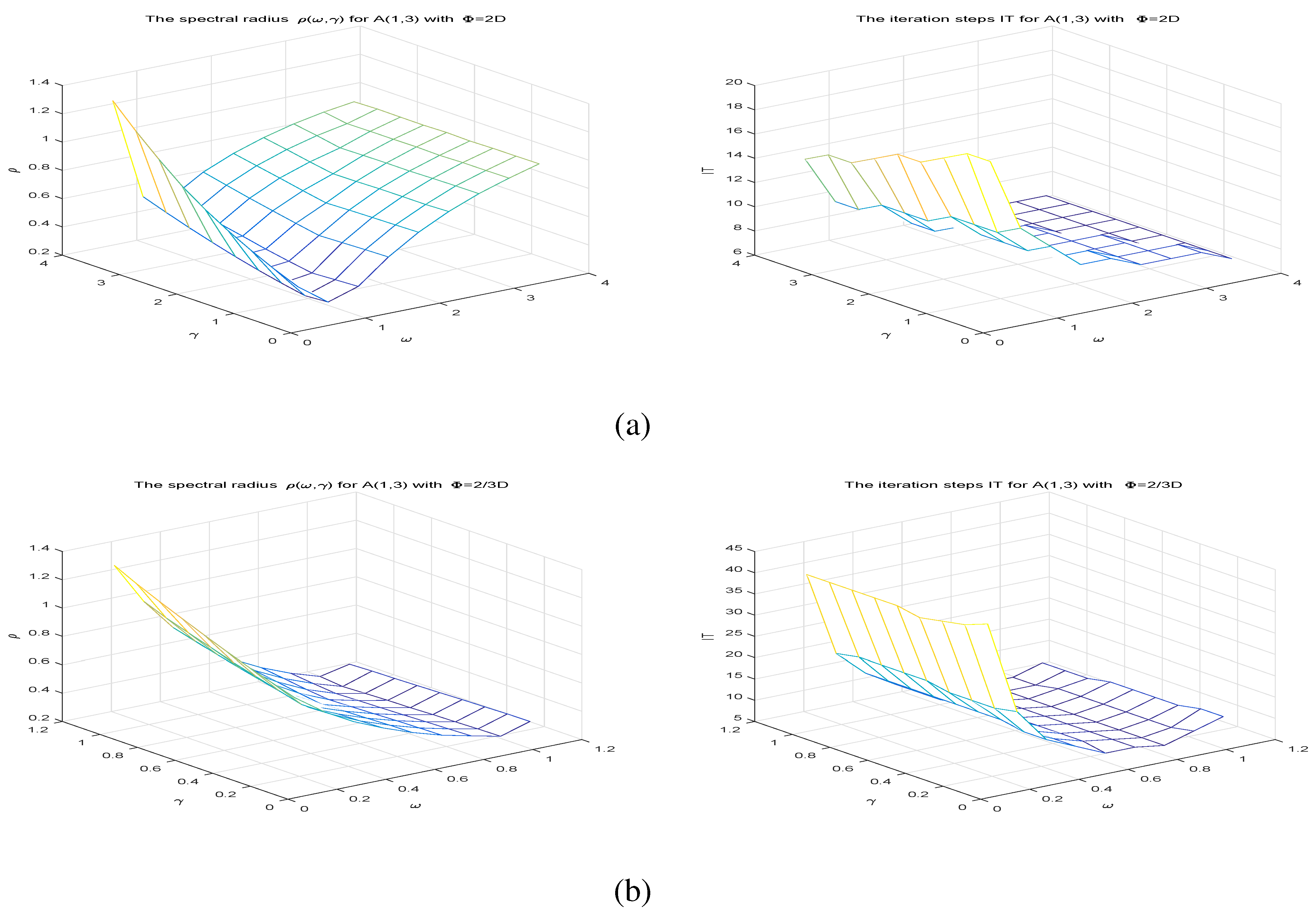
Example 1. 

In this example, we consider the convergence condition of Theorem 3. We let A in the LCP(1) be $A(0,3)$, $A(1,2)$, and $C=\mathrm{diag}\left([1,2,3,1,2,3,\cdots ]\right)\in R^{n\times n}$ with $n=1600$. Then, $A(0,3)$ is a symmetric P-matrix, and $A(1,2)$ is a nonsymmetric P-matrix. We set $\Phi =\varphi I$ with $\varphi >0$ in the TSMMS iteration method (6). For $A(0,2)$, we set

$$F_1=\mathrm{triu}(A,-1)-\mathrm{triu}(A,2)$$

and

$$F_2=A-{(\mathrm{triu}(A,-1)-\mathrm{triu}(A,0))}^{\mathrm{T}}-(\mathrm{triu}(A,-1)-\mathrm{triu}(A,0)).$$

For $A(1,2)$, we set

$$F_1={(\mathrm{triu}(A,-1)-\mathrm{triu}(A,0))}^{\mathrm{T}}+(\mathrm{triu}(A,-1)-\mathrm{triu}(A,1))$$

and

$$F_2={(\mathrm{triu}(A,-m)-\mathrm{triu}(A,0))}^{\mathrm{T}}+(\mathrm{triu}(A,-m)-\mathrm{triu}(A,1)),$$

where “$\mathrm{triu}$” is a function in Matlab. Then, we find that both cases satisfy the conditions (19) and (20) in Theorem 3. So, the convergence region of ϕ is

$$\varphi \in ({\rm Y},+\infty ).$$

To see the numerical results, we set $q=-A{z}^{(*)}$ in the LCP (1), with $z^{(*)}={(1,0,1,0,\cdots )}^{\mathrm{T}}$ being the true solution. We select the values of ϕ in the convergence region, and we denote

$$\sigma =\parallel {({\Phi }_1+F_1)}^{-1}\parallel \left(2\parallel G_1\parallel +\parallel {\Phi }_1-F_1\parallel \right)\parallel {({\Phi }_2+F_2)}^{-1}\parallel \left(2\parallel G_2\parallel +\parallel {\Phi }_2-F_2\parallel \right)$$

(see Theorem 2) and

$$\delta ={\lambda }_1^{\left(1\right)}+{\lambda }_1^{\left(2\right)}-{\tau }^{\left(1\right)}-{\tau }^{\left(2\right)}.$$

Set

$${\rm Y}:1:{\rm Y}+9,$$

and then the convergence domain of ϕ and the numerical results are shown in

Table 1. The convergence domain of $\varphi$ in the TSMMS iteration method.

$\mathit{n}=1600$	$\frac{{\mathit{\lambda }}_1^{\left(1\right)}+{\mathit{\lambda }}_{\mathit{n}}^{\left(1\right)}}{2}$	$\frac{{\mathit{\lambda }}_1^{\left(2\right)}+{\mathit{\lambda }}_{\mathit{n}}^{\left(2\right)}}{2}$	$\mathsf{{\rm Y}}$	$\mathsf{\Gamma }$	$\mathit{\delta }$	$\mathit{\varphi }$
$A(0,3)$	10.00	10.00	5.5367	−1.9941	8.9265	$(5.5367,+\infty )$
$A(1,2)$	8.00	8.00	5.5764	−2.0698	4.8122	$(5.5764,+\infty )$

and

Table 2. The numerical results of the TSMMS iteration method when $\Phi =\varphi I$.

	$A(0,3)$
	${\varphi }_1$	${\varphi }_2$	${\varphi }_3$	${\varphi }_4$	${\varphi }_5$	${\varphi }_6$	${\varphi }_7$	${\varphi }_8$	${\varphi }_9$	${\varphi }_{10}$
$\sigma$	1.00	0.71	0.51	0.35	0.24	0.22	0.25	0.28	0.31	0.33
IT	11	9	7	7	6	6	7	8	9	9
CPU	0.012	0.006	0.004	0.004	0.006	0.003	0.009	0.006	0.009	0.005
	$A(1,2)$
	${\varphi }_1$	${\varphi }_2$	${\varphi }_3$	${\varphi }_4$	${\varphi }_5$	${\varphi }_6$	${\varphi }_7$	${\varphi }_8$	${\varphi }_9$	${\varphi }_{10}$
$\sigma$	1.00	0.66	0.44	0.38	0.42	0.45	0.48	0.51	0.53	0.55
IT	7	6	6	7	8	9	9	10	11	12
CPU	0.025	0.009	0.009	0.011	0.012	0.014	0.014	0.016	0.017	0.019

, as well as Figure 1 below, respectively.

In Figure 1, subfigures (a) and (b) are related to the case $A(0,3)$; subfigures (c) and (d) are related to the case $A(1,2)$. The horizontal axis denotes $\varphi$, and the vertical axis denotes IT and the function $\sigma$, respectively.

Example 2. 

In this example, we consider the convergence of the TSMAOR iteration method. We set A to be $A(1,3)$ with $n=1600$ and C to be same as Example 1. Then, A is an $H_{+}$-matrix, and

$$\rho (D^{-1}\left(\right|L|+\left|U\right|\left)\right)=0.2470<{\displaystyle \frac{1}{2}}.$$

Then, from Corollaries 3 and 4 and Theorem 6, we know that, if $\Phi =2D$, one sufficient region of $\omega ,\gamma$ is

$$0\le \gamma \le \omega \le {\displaystyle \frac{1}{\rho (D^{-1}\left(\right|L|+\left|U\right|\left)\right)}}\mathrm{with}\omega \ne 0,$$

and if $\Phi ={\displaystyle \frac{2}{3}}D$, the sufficient region of $\omega ,\gamma$ is

$$0\le \gamma \le \omega \le {\displaystyle \frac{6}{5}}.$$

In order to see numerical results, we consider some concrete values of $\omega$ and $\gamma$ to perform the TSMAOR iteration method. For $\Phi =2D$, we set

$$\begin{array}{c}\hfill \left\{\begin{array}{c}\omega ={\displaystyle \frac{1}{l\rho }}:{\displaystyle \frac{1}{l\rho }}:{\displaystyle \frac{1}{\rho }}-{\displaystyle \frac{1}{l\rho }},\hfill \\ \gamma ={\displaystyle \frac{1}{l\rho }}:{\displaystyle \frac{1}{l\rho }}:{\displaystyle \frac{1}{\rho }}-{\displaystyle \frac{1}{l\rho }}.\hfill \end{array}\right.\end{array}$$

(28)

For $\Phi ={\displaystyle \frac{2}{3}}D$, we set

$$\begin{array}{c}\hfill \left\{\begin{array}{c}\omega ={\displaystyle \frac{6}{l5}}:{\displaystyle \frac{6}{l5}}:{\displaystyle \frac{6}{5}}-{\displaystyle \frac{6}{l5}},\hfill \\ \gamma ={\displaystyle \frac{6}{l5}}:{\displaystyle \frac{6}{l5}}:{\displaystyle \frac{6}{5}}-{\displaystyle \frac{6}{l5}}.\hfill \end{array}\right.\end{array}$$

(29)

We let $l=10$, and we denote the second conditions’ function (26) in Theorem 6 as

$${\rho }_{(\omega ,\gamma )}=\rho \left(|{({\Phi }_1+F_1)}^{-1}|\left(|G_1|+|A-{\Phi }_1|\right)\left|{({\Phi }_2+F_2)}^{-1}\right|\left(|G_2|+|A-{\Phi }_2|\right)\right).$$

Then, we obtain

Table 3. Numerical results of the TSMAOR iteration method with $\Phi =2D$.

$A(1,3)$
$\rho (\omega ,\gamma )$	${\omega }_1$	${\omega }_2$	${\omega }_3$	${\omega }_4$	${\omega }_5$	${\omega }_6$	${\omega }_7$	${\omega }_8$	${\omega }_9$
${\gamma }_1$	0.428	0.277	0.345	0.511	0.643	0.747	0.831	0.898	0.956
${\gamma }_2$	0.494	0.267	0.337	0.507	0.639	0.741	0.830	0.896	0.955
${\gamma }_3$	0.571	0.299	0.329	0.501	0.636	0.742	0.828	0.897	0.955
${\gamma }_4$	0.655	0.335	0.357	0.496	0.633	0.741	0.824	0.892	0.951
${\gamma }_5$	0.751	0.375	0.387	0.527	0.628	0.737	0.825	0.896	0.956
${\gamma }_6$	0.861	0.421	0.423	0.559	0.659	0.736	0.823	0.895	0.952
${\gamma }_7$	0.994	0.469	0.457	0.593	0.693	0.764	0.821	0.895	0.953
${\gamma }_8$	1.139	0.522	0.497	0.629	0.724	0.796	0.852	0.894	0.955
${\gamma }_9$	1.299	0.578	0.538	0.666	0.756	0.825	0.879	0.920	0.950
IT	${\omega }_1$	${\omega }_2$	${\omega }_3$	${\omega }_4$	${\omega }_5$	${\omega }_6$	${\omega }_7$	${\omega }_8$	${\omega }_9$
${\gamma }_1$	19	13	11	9	9	8	8	8	7
${\gamma }_2$	19	12	10	9	9	8	8	8	7
${\gamma }_3$	18	12	10	9	8	8	8	7	7
${\gamma }_4$	17	12	10	9	8	8	8	7	7
${\gamma }_5$	17	11	10	9	8	8	7	7	7
${\gamma }_6$	16	11	9	9	8	8	7	7	7
${\gamma }_7$	15	11	9	8	8	7	7	7	7
${\gamma }_8$	15	10	9	8	8	7	7	7	7
${\gamma }_9$	14	10	9	8	7	7	7	7	7

and

Table 4. Numerical results of the TSMAOR iteration method with $\Phi ={\displaystyle \frac{2}{3}}D$.

$A(1,3)$
$\rho (\omega ,\gamma )$	${\omega }_1$	${\omega }_2$	${\omega }_3$	${\omega }_4$	${\omega }_5$	${\omega }_6$	${\omega }_7$	${\omega }_8$	${\omega }_9$
${\gamma }_1$	0.821	0.680	0.568	0.480	0.406	0.345	0.298	0.253	0.315
${\gamma }_2$	0.870	0.675	0.565	0.475	0.403	0.341	0.292	0.250	0.314
${\gamma }_3$	0.922	0.718	0.559	0.470	0.397	0.338	0.287	0.245	0.309
${\gamma }_4$	0.979	0.761	0.592	0.464	0.392	0.332	0.281	0.242	0.305
${\gamma }_5$	1.040	0.804	0.629	0.492	0.385	0.326	0.277	0.235	0.300
${\gamma }_6$	1.104	0.855	0.667	0.521	0.408	0.321	0.273	0.232	0.295
${\gamma }_7$	1.170	0.904	0.706	0.553	0.435	0.339	0.268	0.226	0.290
${\gamma }_8$	1.238	0.956	0.749	0.585	0.460	0.361	0.283	0.220	0.287
${\gamma }_9$	1.315	1.019	0.791	0.620	0.485	0.383	0.301	0.236	0.281
IT	${\omega }_1$	${\omega }_2$	${\omega }_3$	${\omega }_4$	${\omega }_5$	${\omega }_6$	${\omega }_7$	${\omega }_8$	${\omega }_9$
${\gamma }_1$	43	21	13	10	7	7	6	8	10
${\gamma }_2$	41	20	13	10	8	7	6	7	10
${\gamma }_3$	40	20	14	10	8	7	6	7	9
${\gamma }_4$	39	20	14	11	8	7	6	7	9
${\gamma }_5$	40	21	14	11	8	7	6	7	9
${\gamma }_6$	40	21	14	11	8	7	6	7	9
${\gamma }_7$	40	21	14	10	8	7	6	7	8
${\gamma }_8$	40	21	14	10	8	7	6	6	8
${\gamma }_9$	40	20	14	10	8	7	6	6	8

, as well as Figure 2, as follows.

In Figure 2, subfigures (a) and (b) correspond to Table 3 and Table 4, respectively, that is, the case $A(1,3)$ with $\Phi =2D$ and the case $A(1,3)$ with $\Phi ={\displaystyle \frac{2}{3}}D$. From Table 3 and Table 4 and Figure 2, we can find that, when $\gamma \le \omega$, the TSMAOR iteration method is convergent, but when $\omega <\gamma$, there are cases in which the convergent condition $\rho (\omega ,\gamma )<1$ is not satisfied, but the TSMAOR iteration method is also convergent. Moreover, the numerical example also shows that the size of the spectral radius $\rho (\omega ,\gamma )<1$ is not exactly consistent with the number of iterative steps (IT), which is shown in sub-figure (a). Moreover, this example also shows that, when $\omega =\gamma$, the TSMGS iteration method usually performs better.

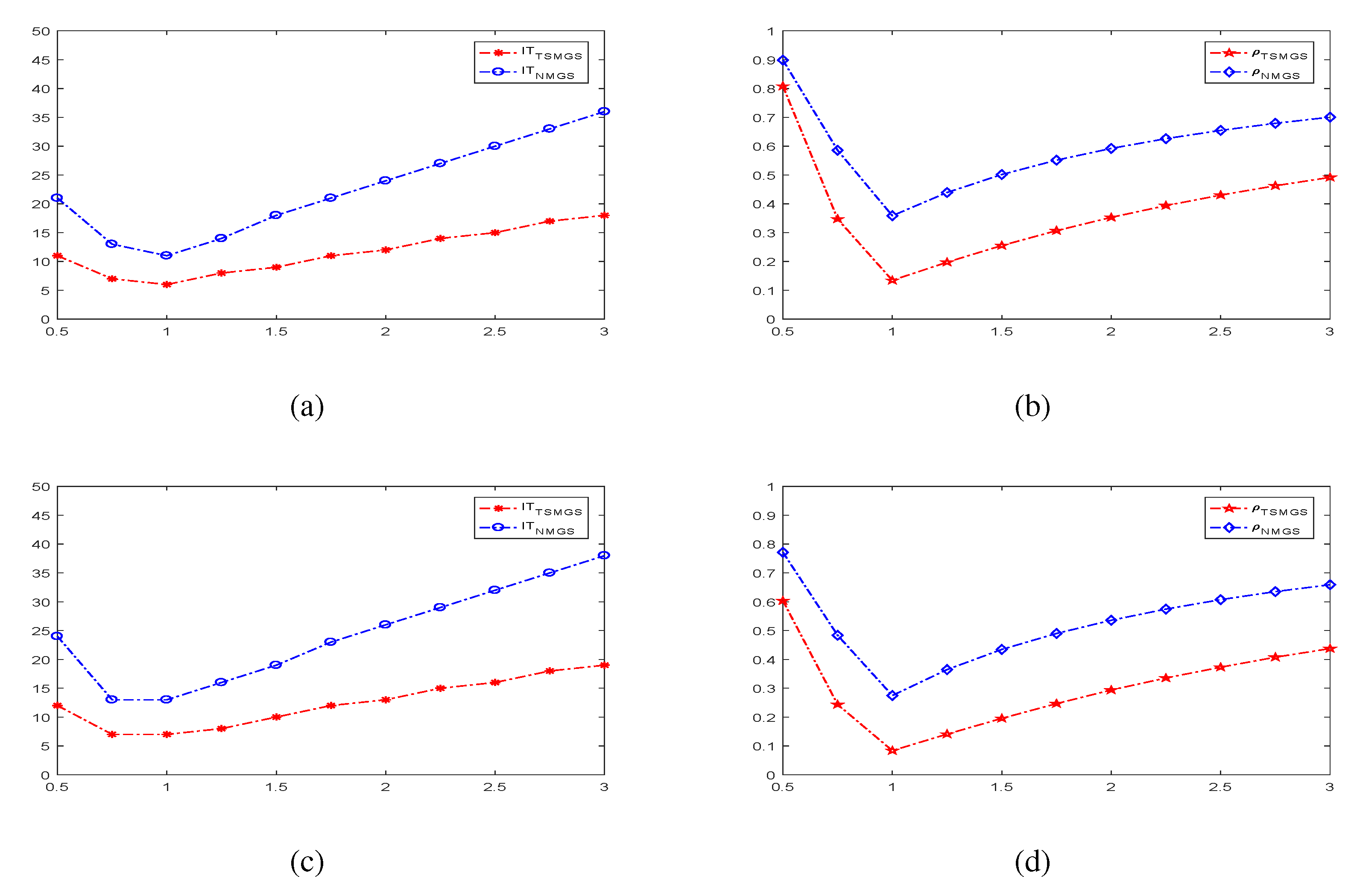
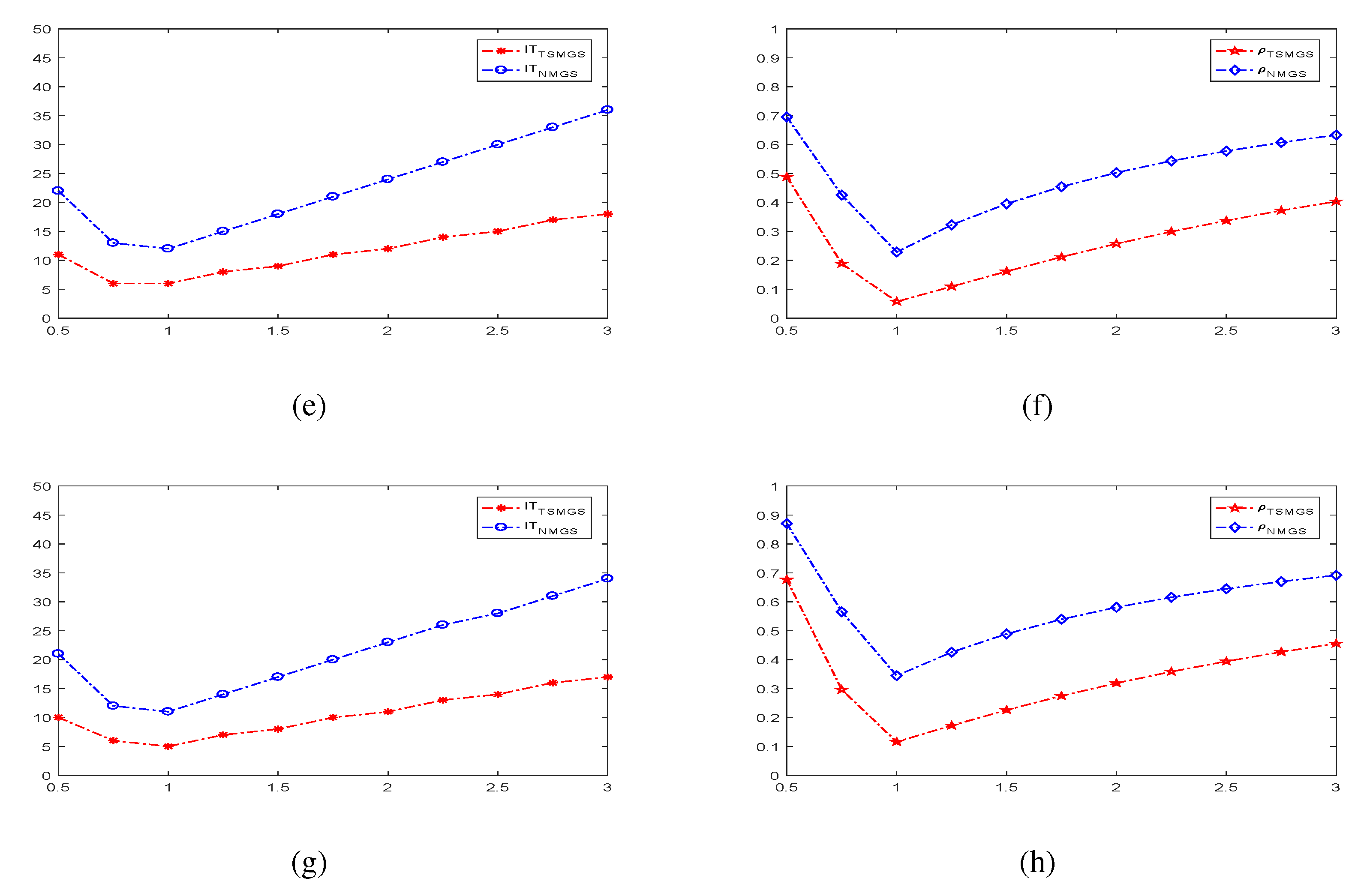
Example 3. 

In this example, we compare the two-step simplified modulus-based Gauss–Seidel (TSMGS) iteration method with the new modulus-based Gauss–Seidel (NMGS) iteration method in [2]. We consider four cases, $A(0,3)$, $A(1,2)$, $A(1,3)$, and $A(2,3)$. We set $n=2500$, and then all four cases satisfy the condition

$$\rho =\rho (D^{-1}\left(\right|L|+\left|U\right|\left)\right)<{\displaystyle \frac{1}{2}}$$

in Corollary 4. Then, the TSMGS iteration method is convergent when $\Phi \ge {\displaystyle \frac{1}{2}}D.$ We set some concrete value of $\Phi$ to perform the two iteration methods, i.e.,

$$\Phi ={\displaystyle \frac{1}{2}}D:{\displaystyle \frac{1}{4}}D:3D.$$

We denote

$${\rho }_{TSMGS}={\rho \left(\right|(\Phi +D-L)}^{-1}{\left|\right(\left|U\right|+|A-\Phi |\left)\right|(\Phi +D-U)}^{-1}\left|\right(\left|L\right|+|A-\Phi |\left)\right)$$

and

$${\rho }_{NMGS}={\rho \left(\right|(\Phi +D-L)}^{-1}\left|\right(\left|U\right|+|A-\Phi |\left)\right),$$

which determine the convergence of the TSMGS iteration method and the NMGS iteration method, respectively. Then, we obtain Figure 3 as follows.

In Figure 3, the horizontal axis denotes $\varphi$ with $\Phi =\varphi D$, and the vertical axis denotes IT. The sub-figures (a) and (b) are related to $A(0,3)$, (c) and (d) are related to $A(1,2)$, (e) and (f) are related to $A(1,3)$, and (g) and (h) are related to $A(2,3)$. This example shows that the TSMGS iteration method is usually better than the NMGS iteration method.

5. Concluding Remarks

We have presented the two-step simplified modulus-based matrix splitting (TSMMS) iteration method for solving the LCP. The general convergence conditions and some concrete convergence conditions were supplied. Numerical experiments verified the effectiveness of the presented method and the convergence conditions. Other complementary problems, such as the implicit complementarity problem and the horizontal linear complementarity problem, can also be considered to use the TSMMS iteration method to reach a solution, which is our future research topic.

References

1. Billups, S.C.; Murty, K.G. Complementarity problems. J. Comput. Appl. Math. 2000, 124, 303–328. [Google Scholar] [CrossRef]
2. Wu, S.L.; Li, C.X. A class of new modulus-based matrix splitting methods for linear complementarity problem. Optim. Lett. 2022, 16, 1427–1443. [Google Scholar] [CrossRef]
3. Ferris, M.C.; Pang, J.S. Complementarity and Variational Problems; State of the Art: Philadephia, PA, USA, 1997. [Google Scholar]
4. Hadjidimos, A.; Lapidakis, M.; Tzoumas, M. On iterative solution for linear complementarity problem with an H+-matrix. SIAM J. Matrix Anal. Appl. 2012, 33, 97–110. [Google Scholar] [CrossRef]
5. Shi, X.J.; Yang, L.; Huang, Z.H. A fixed point method for the linear complementarity problem arising from American option pricing. Acta Math. Appl. Sin. 2016, 32, 921–932. [Google Scholar] [CrossRef]
6. Cottle, R.W.; Sacher, R.S. On the solution of large, structured linear complementarity problems: The tridiagonal case. Appl. Math. Opt. 1976, 3, 321–340. [Google Scholar] [CrossRef]
7. Zheng, N.; Hayami, K.; Yin, J.F. Modulus-type inner outer iteration methods for nonnegative constrained least squares problems. SIAM J. Matrix Anal. Appl. 2016, 37, 1250–1278. [Google Scholar] [CrossRef]
8. Bai, Z.Z. Modulus-based matrix splitting iteration methods for linear complementarity problems. Numer. Linear Algebra Appl. 2010, 17, 917–933. [Google Scholar] [CrossRef]
9. Li, W. A general modulus-based matrix splitting method for linear complementarity problems of H-matrices. Appl. Math. Lett. 2013, 26, 1159–1164. [Google Scholar] [CrossRef]
10. Zheng, N.; Yin, J.F. Accelerated modulus-based matrix splitting iteration methods for linear complementarity problem. Numer. Algor. 2013, 64, 245–262. [Google Scholar] [CrossRef]
11. Zhang, L.L. Two-step modulus-based matrix splitting iteration method for linear complementarity problems. Numer. Algor. 2011, 57, 83–99. [Google Scholar] [CrossRef]
12. Cvetković, L.; Hadjidimos, A.; Kostić, V. On the choice of parameters in MAOR type splitting methods for the linear complementarity problem. Numer. Algor. 2014, 67, 793–806. [Google Scholar] [CrossRef]
13. Zheng, H.; Cui, J.J. Accelerated relaxation two-sweep modulus-based matrix splitting iteration method for linear complementarity problems. Int. J. Comp. Meth. 2024, 21, 2350025. [Google Scholar]
14. Zheng, H.; Vong, S. A modified modulus-based matrix splitting iteration method for solving implicit complementarity problems. Numer. Algor. 2019, 82, 573–592. [Google Scholar] [CrossRef]
15. Fang, X.M. The convergence of modulus-based matrix splitting iteration methods for implicit complementarity problems. Comput. Appl. Math. 2022, 411, 114241. [Google Scholar] [CrossRef]
16. Mezzadri, F.; Galligani, E. Modulus-based matrix splitting methods for a class of horizontal nonlinear complementarity problems. Numer. Algor. 2021, 87, 667–687. [Google Scholar] [CrossRef]
17. Mezzadri, F.; Galligani, E. Modulus-based matrix splitting methods for horizontal linear complementarity problems. Numer. Algor. 2020, 83, 201–219. [Google Scholar] [CrossRef]
18. Liao, S.W.; Zhang, G.F.; Liang, Z.Z. A preconditioned general modulus-based matrix splitting iteration method for solving horizontal linear complementarity problems. Numer. Algor. 2023, 93, 919–947. [Google Scholar] [CrossRef]
19. Guo, W.X.; Zheng, H.; Peng, X.F. New convergence results of the modulus-based methods for vertical linear complementarity problems. Appl. Math. Lett. 2023, 135, 108444. [Google Scholar] [CrossRef]
20. Mezzadri, F. A modulus-based formulation for the vertical linear complementarity problems. Numer. Algor. 2022, 90, 1547–1568. [Google Scholar] [CrossRef]
21. Zheng, H.; Zhang, Y.X.; Lu, X.P.; Vong, S. Modulus-based synchronous multisplitting iteration methods for large sparse vertical linear complementarity problems. Numer. Algor. 2023, 93, 711–729. [Google Scholar] [CrossRef]
22. Hong, J.T.; Li, C.L. Modulus-based matrix splitting iteration methods for a class of nonlinear complementarity problem. Appl. Math. Comput. 2016, 23, 629–641. [Google Scholar] [CrossRef]
23. Huang, N.; Ma, C.F. The modulus-based matrix splitting algorithms for a class of weakly nonlinear complementarity problems. Numer. Linear Algebra 2016, 23, 558–569. [Google Scholar] [CrossRef]
24. Wang, G.B.; Tan, F.P. Modulus-based multisplitting iteration method for a class of weakly nonlinear complementarity problems. Comput. Appl. Math. Comput. 2021, 3, 419–428. [Google Scholar] [CrossRef]
25. Fang, X. Convergence of modulus-based matrix splitting iteration method for a class of nonlinear complementarity problems. Numer. Algor. 2022, 90, 931–950. [Google Scholar] [CrossRef]
26. Sharaf, I.M. A projection algorithm for positive definite linear complementarity problems with applications. Int. J. Manag. Sci. Eng. 2016, 12, 141–147. [Google Scholar] [CrossRef]
27. Zheng, H.; Li, W. The modulus-based nonsmooth Newton’s method for solving linear complementarity problems. J. Comput. Appl. Math. 2015, 288, 116–126. [Google Scholar] [CrossRef]
28. Fang, X.M. The simplified modulus-based matrix splitting iteration method for the nonlinear complementarity problem. AIMS Math. 2024, 9, 8594–8609. [Google Scholar] [CrossRef]
29. Frommer, A.; Szyld, D.B. H-splittings and two-stage iterative methods. Numer. Math. 1992, 63, 345–356. [Google Scholar] [CrossRef]
30. Varga, R.S. Matrix Iterative Analysis; Springer: Berlin/Heidelberg, Germany, 2000. [Google Scholar]
Figure 1. Comparison of IT and σ for Method 1 with Φ = ϕ I .
Symmetry 16 01210 g001
Figure 2. Comparison of IT and the spectral radius ρ ( ω , γ ) in the TSMAOR iteration method.
Symmetry 16 01210 g002
Figure 3. Comparison between the TSMGS iteration method and the NMGS iteration method.
Symmetry 16 01210 g003aSymmetry 16 01210 g003b