Real-Time Control of Sintering Moisture Based on Temporal Fusion Transformers

Abstract

The quality of sintered ore, which serves as the primary raw material for blast furnace ironmaking, is directly influenced by the moisture in the sintering mixture. In order to improve the precision of water addition in the sintering process, this paper proposes an intelligent model for predicting water-filling volume based on Temporal Fusion Transformer (TFT), whose symmetry enables it to effectively capture long-term dependencies in time series data. Utilizing historical sintering data to develop a prediction model for the amount of mixing and water addition, the results indicate that the TFT model can achieve the R squared of 0.9881, and the root mean square error (RMSE) of 3.5951. When compared to the transformer, long short-term memory (LSTM), and particle swarm optimization–long short-term memory (PSO-LSTM), it is evident that the TFT model outperforms the other models, improving the RMSE by 8.5403, 6.9852, and 0.453, respectively. As an application, the TFT model provides an effective interval reference for moisture control in normal sintering processes, which ensures that the error is within 1 t.

1. Introduction

The automation and intelligent control of the entire sintering production process has become a prevailing trend [1]. The iron-sintering process involves mixing iron ore, fluxes and fuels in specific proportions and adding the appropriate amount of water [2]. The water content during the sintering process not only significantly affects the quality of the sintered ore but also impacts the production efficiency [3]. The traditional sintering process primarily relies on manual estimation by employees to control the water injection, leading to high variations in moisture content [4]. Since the empirical model is influenced by manual operation parameters, it is important to establish a more optimized water-adding volume control model to realize the automation and intelligent control of the water addition process.

In some study on the intelligent control of the sintering process, Li and Gong [5] proposed an adaptive fuzzy PID control system to address the time lag phenomenon and parameter uncertainty of the sintering process. However, the adaptive fuzzy PID model is sensitive to the selection of fuzzy sets and relies on manual experience. Giri and Roy [6] introduced a sintering process control system based on genetic algorithms to optimize the parameters of the PID model, but the complexity of the energy balance calculation makes the model challenging to apply. Artificial neural networks have been widely utilized in the field of sintering moisture prediction due to their ability to recognize nonlinear relationships. Cai [7] proposed a feedforward water addition model based on the least squares method to control the material balance, which can control the moisture content of the mixture during the sintering process; however, under the given mixed ore structure, the water absorption capacity of the mixture and the role of moisture in the granulation effect were ignored. Jiang et al. [8] proposed a NARX control system based on the combination of offline and online approaches, but there is room for improvement in the prediction accuracy of the model. Ren et al. [9] utilized the KPCA-GA model based on the BP neural network, which had better prediction accuracy compared to the traditional neural network model. But the model lacks interpretation and numerical prediction, and it is difficult to achieve the precise control of moisture.

In recent years, deep neural network architectures have been gradually applied in various fields, and the LSTM model is widely used in the field of time series prediction. The Transformer model, on the other hand, due to its stronger long-term memory capability and nonlinear mapping advantage, has also been successfully applied to many fields such as image recognition [10,11], medical data processing [12,13], and text processing [14,15], etc. However both models suffer from defects that are difficult to interpret. In 2021, Google proposed an improved Temporal Fusion Transformer (TFT) model [16], which improves on the Transformer model. The adequate consideration of different types of inputs makes the model more accurate in the prediction of nonlinear relationships, and it utilizes the attention mechanism to make the model interpretable. This paper argues that the symmetry of TFT is reflected in three aspects: time, characteristics and attention. Time series can be divided into past and future parts by symmetry in time because past events affect the occurrence of future events; our hypothesis is that the features in the time series are symmetrical and therefore the same in the choice of encoder and decoder. The symmetry of the self-attention mechanism is understood in this paper to mean that it is possible to focus on both past and future features, and the dependence between such data features can be captured. From this point of view, it can be argued that TFT captures the long-term dependencies between the past and the future in the data, making more accurate predictions, and the same decoder and encoder can reduce the complexity of the model. The advantages of the TFT model for nonlinear systems and the recognition of unexpected events by its attention mechanism make it possible to deal with sintering and water addition processes with transient on–off phenomena.

Therefore, in this study, a real-time prediction and control model for the addition of water to sintering is developed, and the results of the model are interpretable based on the attention mechanism from three perspectives: input characteristics, time, and abnormal working conditions. The main contributions of this paper are as follows:

1. A novel model for predicting sintering water addition parameters is proposed for the intelligent control of water addition in the sintering process, which combines multi-horizon forecasting with interpretability into temporal dynamics and utilizes the gating layers to suppress unnecessary components;

2. Interpretability analyses are conducted for the water addition model to investigate the effects of different materials, time of day, and contingencies on the amount of water added.

2. Sintering and Water Addition Process Mechanism

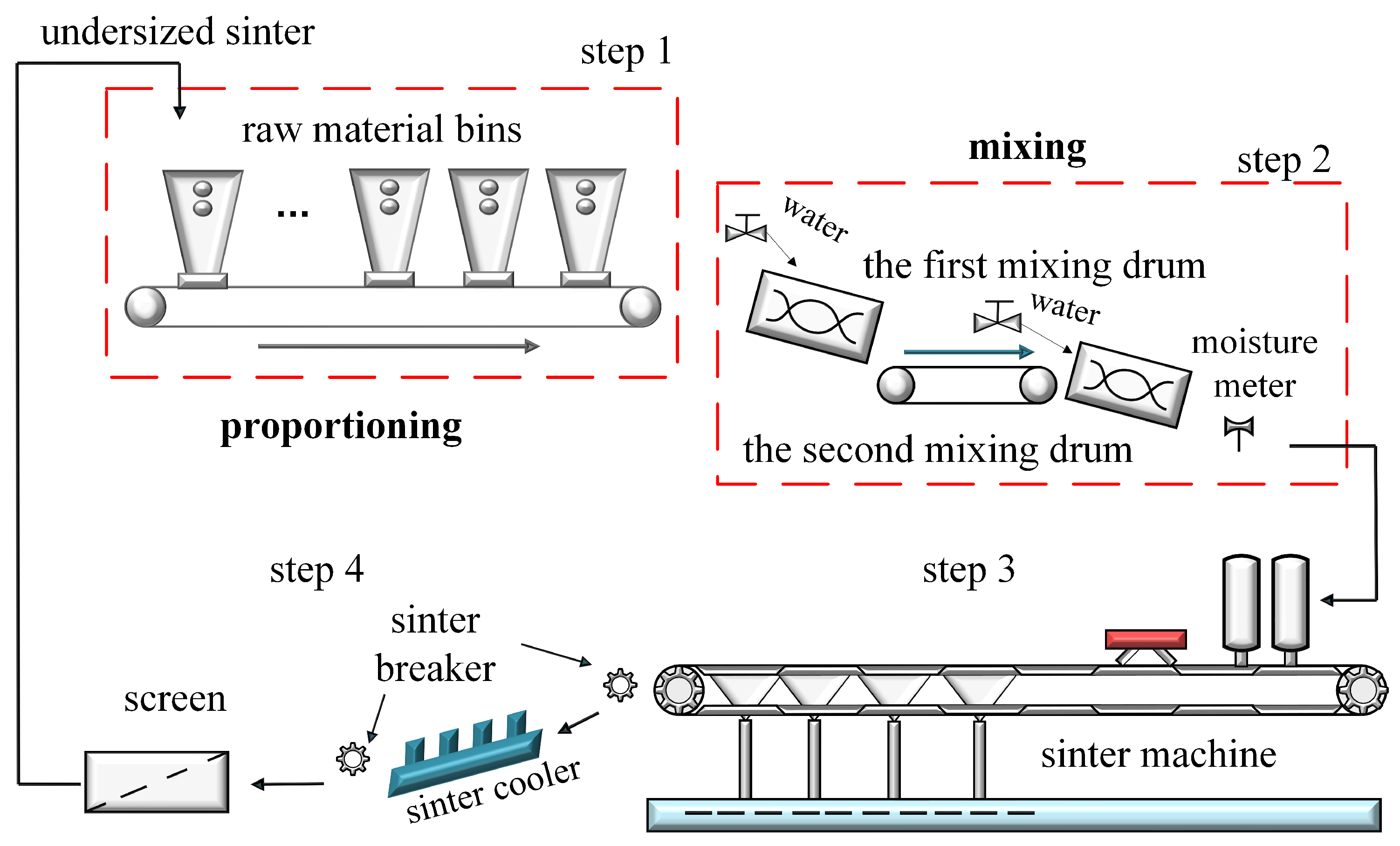
In the sintering process, the model of the actual mixer is shown in Figure 1. The whole sintering process can be divided into four steps: the first part is the batching, the second part is the mixing, the third part is the ignition high-temperature sintering, and the fourth part is the crushing, screening and cooling of the material. In the first step, various raw materials are placed in different containers, and the required raw materials are taken out in proportion to the conveyor belt under computer control, such as iron ore, dolomite, quicklime, etc. Then, enter the second step, the process can be divided into two mixing steps; this paper will mainly introduce and study this step. In the third step, the mixed raw material continues through the sintering machine for a series of operations, and the sintering process ends when the reaction in the unit reaches the end. In the fourth step, the sintered ore is crushed and sieved according to size and cooled in a cooler. After screening, the qualified sinter is sent to the blast furnace to make iron, while the unqualified part is returned to the batching area of step 1 for the next round of sintering. This paper focuses on the second step of the whole sintering process: mixing.

In the second step, there are two mixing drums, and various raw materials are first introduced into the first mixing drum, at which time the inlet valve adds water to the raw material mixture and mixes it fully to form the raw material mixture. The initial addition of materials includes sintered return ore, limestone, quicklime, dolomite, iron ore, etc. The raw materials are then transferred to a second mixing drum for mixing, and the second mixing is for granulation. The inlet valve also adds water to the raw material mixture and mixes it. There is a moisture meter at the end of both mixing drums to measure the moisture content in the mixture. The operator will dynamically adjust the amount of water added in the second inlet valve according to the quantity of raw materials and moisture content measured by the moisture meter so that the moisture content of the mixture coming out of the second mixing drum can reach the standard [8].

During the sintering process, various materials are introduced into the sintering machine, which then enter the mixer and combine with water to create a raw material mixture. Initially the added materials include sintered ore return, limestone, quicklime, dolomite, iron ore return, etc. After the raw materials are mixed, the water content in the mixture is measured at two points where water is added. At this stage, the worker will adjust the amount of water to be added based on the quantity of material and the moisture content measured by the hydrometer [8].

The water content of the raw material mixture is theoretically calculated as follows:

$$M={\displaystyle \frac{{\sum }_{i=1}^n{K}_i\times W_i+U+U_r}{{\sum }_{i=1}^n{W}_i+U+W_r}}$$

(1)

where M represents the water content of the mixture, $W_i$ denotes the weight of each raw material in the mixture, $W_r$ and $U_r$ indicate the weight and water content of the sintered ore, U signifies the amount of artificially added water, and $K_i$ represents the water content of the material. The units for M, $W_i$, $W_r$ and $U_r$ are $t/h$, and the unit for $K_i$ is %. Therefore, it can be concluded that the quantity of artificially added water should be:

$$U={\displaystyle \frac{M\times [{\sum }_{i=1}^n{W}_i+W_r]-[{\sum }_{i=1}^n{K}_i\times W_i+U_r]}{1-M}}$$

(2)

The amount of water added is controlled so that the water content of the mixture meets the optimal demand, and the amount of water added to the mixer at a given moment correlates with the amount added in the previous period. This correlation allows for controlling the water addition in the sintering process based on the previous amount added and the measured material quantity:

$$U(i+1)=g(u_1\left(i\right),u_1(i-1),\dots ,u_1(i-d_x)),$$

(3)

$${u_1}^T=[U_1,U_2,\dots ,U_n]$$

(4)

The control system for adding water during sintering becomes a complex nonlinear system due to the delay between measuring the material quantity and the actual fabric in the sintering process, and the influence of the raw material water content and moisture measurement values by the ambient temperature and humidity. The main objective of this study is to analyze and predict the complex nonlinear system using the Temporal Fusion Transformers (TFTs).

3. Model Architecture

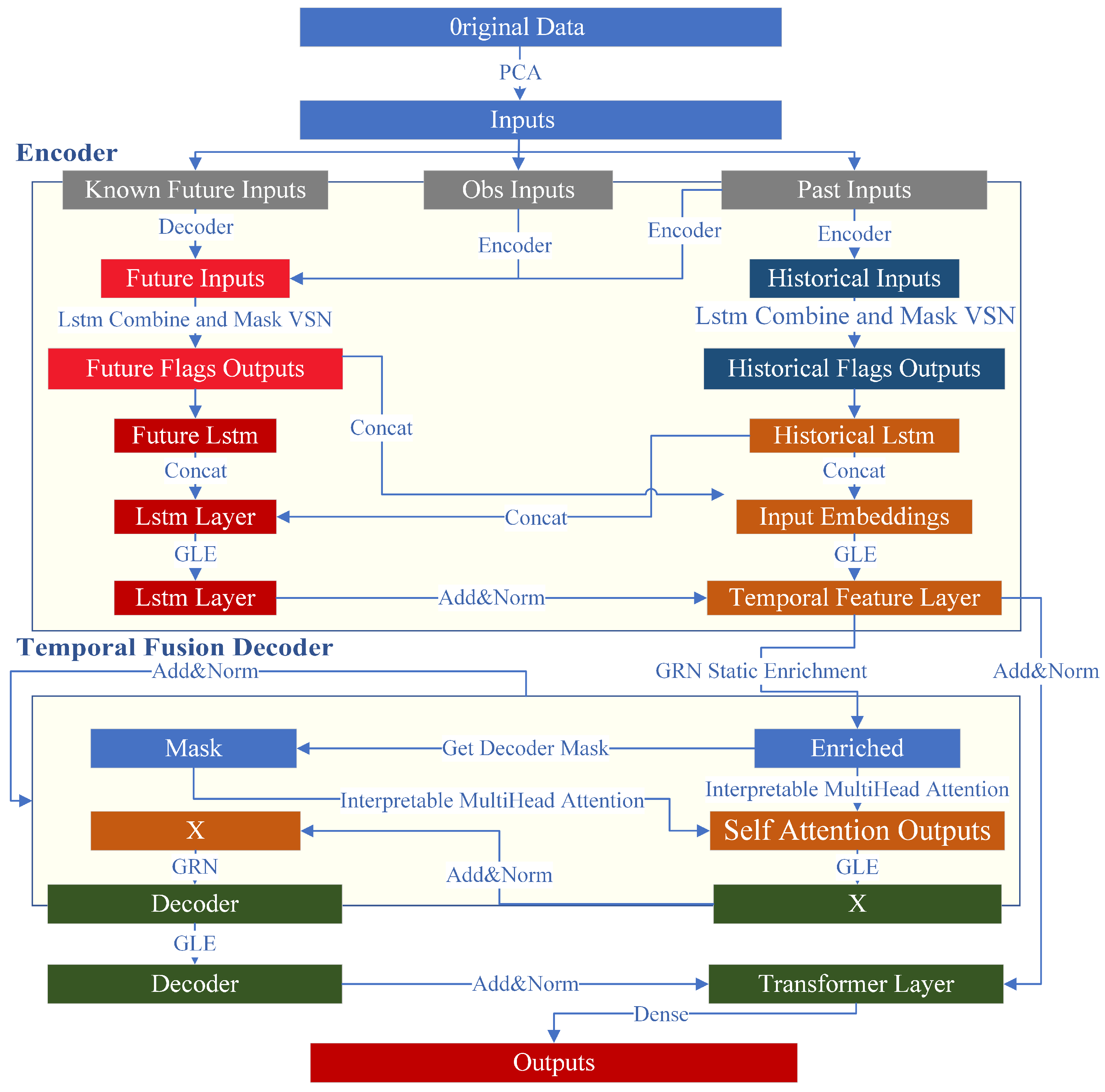
The TFT water addition control model used in this paper is shown in Figure 2, the model first uses principal component analysis to downscale the features obtained in the sintering process. Subsequently, the features are downscaled into the variable selection network (VSN) to identify the significant features.The model then utilizes LSTM to process temporal information, and the long-term dependency in the processing is analyzed using the multi-head attention mechanism. The Gated Residual Network (GRN) is designed to skip unused components of the architecture in order to manage the depth and complexity of the model. The entire prediction process uses a quantized loss function to calculate the model’s prediction error.

3.1. Gated Residual Networks

The Gated Residual Network (GRN) is primarily utilized to address the challenge of determining the extent of nonlinear processing resulting from the uncertain relationship between exogenous inputs and the target. This allows the model to apply nonlinear processing only when the exogenous inputs are strongly correlated with the target outputs. The GRN uses a group of Gated Linear Units (GLUs) to enable the component gating layer to bypass unnecessary components in the model architecture, thereby controlling model complexity and providing self-adaptation depth.

The formula for GRN is as follows:

$$\begin{array}{cc}\hfill GR{N}_{\omega }(a,c)& =LayerNorm(a+GL{U}_{\omega }\left({\eta }_1\right)),\hfill \end{array}$$

(5)

$$\begin{array}{cc}\hfill {\eta }_1& =W_{1,\omega }{\eta }_2+b_{1,\omega },\hfill \end{array}$$

(6)

$$\begin{array}{cc}\hfill {\eta }_2& =ELU(W_{2,\omega }a+W_{3,\omega }c+b_{2,\omega })\hfill \end{array}$$

(7)

ELU is an exponential linear unit activation function that mitigates the “dead zone” issue of Relu when the input is less than 0, making it more robust to input changes or noise. The linear component on the right side also addresses the problem of the vanishing gradient that occurs with the Sigmoid function. The intermediate layers include LayerNorm as the normalization criterion layer, and $\omega$ indicates an indicator of weight sharing.

3.2. Variable Selection Network

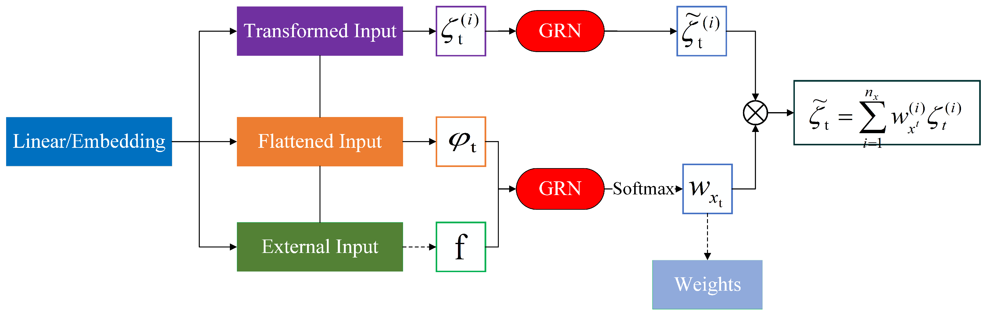
Most real-time series data contain only a few features directly related to the prediction target, along with time-varying covariates that change with the input features. Variable selection networks (as shown in Figure 3) analyze the importance of the input variables to the prediction target and eliminate noisy inputs that negatively impact the model’s performance. This process greatly improves the model’s performance by focusing on learning the most significant features using a learning mechanism.

An entity embedding representation is utilized for the categorical variables, while linear transformations are applied to the continuous variables. All input variables are then transformed into d-dimensional vectors to match the subsequent layer inputs. Let ${\zeta }_t^{\left(i\right)}$ denote the transformed j-th input variable at time t. Then, ${\psi }_t=[{{\zeta }_t^{\left(1\right)}}^T,{{\zeta }_t^{\left(2\right)}}^T,\dots ,{{\zeta }_t^{\left(n_x\right)}}^T]$ denotes the vector of all input features at time t. This vector and the external context vector c are acted upon by the Gated Residual Network and input to the Softmax function to determine the variable selection weights, and the formula is as follows:

$$w_{x_t}=Softmax\left(GR{N}_{w_x}({\psi }_t,c_s)\right)$$

(8)

For each time step, the GRN is used for nonlinear processing with the following equations:

$${\widetilde{{\zeta }_t}}^{\left(j\right)}=GR{N}_{\tilde{\zeta }\left(j\right)}\left({{\zeta }_t}^{\left(j\right)}\right)$$

(9)

where ${\widetilde{{\zeta }_t}}^{\left(j\right)}$ denotes the feature vector of variable j after the action of GRN, and the weights obtained by each variable through its own GRN are applicable at all time steps. At the end of the feature selection network, the variable weights will influence their corresponding transformation variables.

3.3. Interpretable Multi-Head Attention

The self-attentive mechanism utilizes its input features and the learnable parameters of the neural network to generate the corresponding query vector Q, key vector K, and value vector V^[19]. Where $Q=[q_1,q_2,\dots ,q_D]$, $K=[k_1,k_2,\dots ,k_D]$ and $V=[v_1,v_2,\dots ,v_D]$, using the normalization function and the scaled dot product as the scoring function, the result of the self-attention is:

$$ATT=Softmax\left({\displaystyle \frac{Q{K}^T}{\sqrt{d_{attn}}}}\right)$$

(10)

The multi-head attention mechanism is designed based on the self-attention mechanism and employs multiple attention heads, each capable of capturing the interaction information of different characteristics. This effectively improves the learning ability of the standard attention mechanism. The model of the multi-head attention mechanism is as follows:

$$Multihead\left(H\right)=[AT{T}_1\oplus AT{T}_2\oplus \cdots \oplus AT{T}_m]W_h$$

(11)

where m represents the number of attention heads.

To represent feature importance, multiple attention heads were designed to share the value of each attention head instead of each having a different value. The shared value was determined through the additive aggregation of each attention head:

$$\begin{array}{cc}\hfill & InterpretableMultihead\left(H\right)=\widetilde{ATT}{W}_h\hfill \end{array}$$

(12)

$$\begin{array}{cc}\hfill & \widetilde{ATT}=\tilde{A}(Q,K)V{W}_v,\hfill \end{array}$$

(13)

$$\begin{array}{cc}\hfill & =\{1/H\sum _{h=1}^{m_H}A(Q{W_Q}^{\left(h\right)},K{W_K}^{\left(h\right)})\}V{W}_V,\hfill \end{array}$$

(14)

$$\begin{array}{cc}\hfill & =1/H\sum _{h=1}^{m_H}Attention(Q{W_Q}^{\left(h\right)},K{W_K}^{\left(h\right)},V{W}_V)\hfill \end{array}$$

(15)

where $W_V$ represents the shared weight value of the attention head in the multi-head attention mechanism and $W_h$ is used to realize the linear mapping.

3.4. Temporal Fusion Decoder

3.4.1. Local Enhanced Sequence Layer

The significance of a point in time series data is often determined by the surrounding data, such as the position of variations. Peaks in data have periodic variations. The performance of the attention-based architecture model can be improved by integrating contextual features through pointwise computation. Due to the fluctuating number of past and future feature inputs, it is not feasible to extract local patterns using a filter with a single convolutional layer. The locally enhanced sequence layer can be handled by inputting ${\tilde{\xi }}_{t-k:t}$ into the LSTM encoder and ${\tilde{\xi }}_{t+1:t+{\tau }_{max}}$ into the LSTM decoder. This process produces a consistent temporal feature $\varphi (t,n)\in \{\varphi (t,-k),\dots ,\varphi (t,{\tau }_{max})\}$:

$$\tilde{\varphi }(t,n)=LayerNorm({\tilde{\xi }}_{t+n}+GL{U}_{\tilde{\varphi }}\left(\varphi (t,n)\right))$$

(16)

3.4.2. Static Enrichment Layer

The static enrichment layer enhances temporal characterization by utilizing static metadata to reflect the significant impact of static covariates on time-varying characteristics. For example, it can demonstrate how the material moisture content is affected by geographic variation. It is calculated using the formula:

$$\theta (t,n)=GR{N}_{\theta }(\tilde{\varphi }(t,n),c_e)$$

(17)

where n denotes the index of the static metadata, GRN weights are shared across the static enrichment layer, and $c_e$ corresponds to the context vector of the encoder.

3.4.3. Temporal Self-Attention Layer

The temporal self-attention layer allows the model to capture long-term temporal dependencies by utilizing the multi-attention mechanism on temporal features. It also incorporates the decoder masking principle with a gating layer to ensure that each temporal dimension focuses solely on events occurring before the current time node. The calculation formula is as follows:

$$\mathit{B}\left(t\right)=InterpretableMultiHead(\Theta (t),\Theta (t),\Theta (t\left)\right),$$

(18)

$$\mathit{\delta }(t,n)=LayerNorm(\mathit{\theta }(t,n)+GL{U}_{\delta }\left(\mathit{\beta }(t,n)\right))$$

(19)

where $\Theta \left(t\right)$ denotes the separate grouping matrix of the static time features and $\mathit{B}\left(t\right)=\left[\mathit{\beta }\right(t,-k),\dots ,\mathit{\beta }(t,{\tau }_{max}\left)\right]$.

3.4.4. Position-Wise Feedforward Layer

The positional feedforward layer is similar to the static enrichment layer and serves as a nonlinear transformation of the output from the temporal self-attention layer. Its computational formula is:

$$\psi (t,n)=GR{N}_{\psi }\left(\mathit{\delta }(t,n)\right)$$

(20)

At the same time, the TFT model considers the scenario in which the model does not require the application of the temporal fusion transformers. In this case, a gated residual connection is established to bypass the entire fusion transformer module. The model will then be simplified as:

$$\tilde{\psi }(t,n)=LayerNorm(\tilde{\varphi }(t,n)+GL{U}_{\tilde{\psi }}\left(\psi (t,n)\right))$$

(21)

3.5. Quantile Regression Loss Function

The traditional linear regression model applies to the conditional distribution of the dependent variable based on the independent variable X. In real-world applications, the least squares method may be less stable and more prone to instability when the data exhibit a distribution with sharp peaks or thick tails, as well as significant heteroskedasticity.

Compared with the traditional linear regression model, quantile regression offers greater robustness, improved flexibility, and stronger resistance to anomalies in the data. Unlike ordinary least squares regression, quantile regression applies a monotonic transformation to the dependent variable. Additionally, the parameters estimated by quantile regression demonstrate asymptotic excellence under the theory of large samples.

The formula for the loss function kernel in quantile regression is generally as follows:

$$max(q\times (y-y_{pred}),(1-q)\times (y_{pred}-y))$$

(22)

In a regular MSE, the loss per sample is ${(y-y_{pred})}^2$, whereas here, $y-y_{pred}$ and $y_{pred}-y$ are one positive and one negative.

4. TFT Sintering Mositure Model

4.1. Data Pre-Processing

The determination of the sintering water addition is primarily based on the real-time monitoring of the material volume and the moisture content. Factors affecting the water content also include the mixing efficiency of the mixer, fluctuations in the water content, the system turnover index, and the sintering environment [9]. Given that the mixing efficiency of the mixer is a controllable factor for the plant and that environmental factors are less variable for the determination of the plant, the assumptions in this article are only focused on analyzing the impact of material volume and moisture content on the amount of sintering water added under specific ambient temperature and mixing efficiency conditions.

The data used in the experiments in this paper are all from the real-time monitoring system of the plant (the volume of the sintering machine is 360 m², the volume of the mixed hopper is in tons, and the measuring accuracy of the moisture meter is 0.001). They contain the plant’s sintering system measurement data from January 2018 to April 2018. The data were collected every 4 s, totaling 1,636,000 entries (as shown in

Table 1. Historical data used in the experiment.

Time (s)	Limestone (t/h)	Quicklime (t/h)	⋯	Moisture (%)	Added Water (t/h)
0	229	76	⋯	7.4	115
4	232	67	⋯	7.4	115
8	237	56	⋯	7.4	114
12	230	54	⋯	7.5	113
16	224	62	⋯	7.4	113
⋯	⋯	⋯	⋯	⋯	⋯

), in which the amount of artificial added water is the predicted output variable of the model, and the remaining variables include the amount of each type of material in the sintering process with real-time moisture measurements as input variables.

The raw sintering data contain a variety of materials, and there is a correlation between the inputs of each material. In order to make the model results more accurate, the dimensionality of the input features was chosen to be reduced. The Bartlett’s test corresponds to a p-value of less than 0.05, indicating that each material quantity is suitable for principal component analysis. Therefore, we use principal component analysis to extract a total of nine materials as the main factors affecting the water addition process (shown in Figure 4); it can be seen that the input of each material quantity in the sintering process is a basically stable process.

Figure 5 shows the correlation between the principal component. Based on the correlation coefficients between the amount of each mixture and the moisture content of the sinter ore, it is concluded that there is a correlation between the sinter ore moisture content (Mo) and quicklime (Qu) inputs, with a correlation coefficient of 0.44. The sintered returned ore (Si) and limestone (Li) showed a correlation coefficient of 0.42 with the moisture measurements (Mo). At the same time, there is a positive correlation between the amount of each material input and the moisture content, and there is no negative correlation, which is consistent with the observation that an increase in the amount of material input is accompanied by a corresponding increase in water content.

The data need to be normalized because of the significant variations in the weights of the different sintered material inputs. In the sintering process, it is typical for the sintering machine to start running and shut down when the material amount reaches zero. Therefore, no specific treatment of this occurrence is conducted during the modeling process to allow the model to understand the actual sintering and water addition process, thereby guiding the water addition process. Moreover, the strength of the TFT model also lies in its ability to account for special events, which will be discussed in the model interpretability section of this paper.

4.2. TFT Network Architecture and Training Result Analysis

After reducing the dimensionality of the above data through principal component analysis, the TFT model is constructed using the model architecture proposed by Google [16]. The model contains 11 input variables and culminates in the amount of water added as an output.

Table 2. Table of model parameters.

Model Parameters	Value
Learning rate	0.001
Number of iterations	15
Number of attention heads	4
Encoding time step	168
Total time step	192
Number of single batches	36

lists the model parameters. The dataset is divided into 90% for training samples, 5% for validation samples, and 5% for test samples.

As depicted in

Table 3. Indicators for assessing model results.

Time Interval (s)	RMSE	RMSEr	R
0	3.5651	0.0298	0.9940
4	4.0208	0.0334	0.9924
8	4.4209	0.0367	0.9907
12	4.6186	0.0383	0.9899
16	4.4401	0.0369	0.9895
⋯	⋯	⋯	⋯

, the root mean square error (RMSE) and relative RMSE (RMSEr) between the predicted values and the actual values obtained from the water addition prediction model based on the TFT model are low. This indicates that the model can effectively minimize prediction errors and more accurately regulate the amount of water added during the sintering process.

Since the instant-on and instant-off process of sintering water addition is affected by humans, in order to accurately evaluate the prediction effect of the model on the water addition, the human interference is considered when assessing the degree of fit.The analysis reveals a slight increase in model error as the number of steps increases, but the overall change is small, which can more accurately determine the water filling volume control. However, the most accurate model predictions were made with fewer steps, and the results for steps 1 and 2 are shown in Figure 6.

A comparison of the predicted results with the true values using the TFT model is shown in

Table 4. TFT model predictions.

Times (s)	True Added Water	P50 Added Water	P90 Added Water
0	114	114.4302	114.9393
4	114	114.4522	114.9517
8	114	114.4081	114.9467
12	114	114.4565	114.9686
16	115	115.5932	116.1918
⋯	⋯	⋯	⋯

. It is evident that when the percentile loss is 50%, there is a more accurate prediction of the required amount of water to be added. On the other hand, a 90th percentile quartile ensures that the actual amount of water to be added meets a 90% probability to be less than the predicted amount. This provides an upper limit guide for the water addition process.

4.3. Comparative Analysis with Existing Models

To further analyze the TFT model’s ability to regulate the amount of water added during the sintering process, we compare the effectiveness of the TFT sintering water addition model with other time series prediction models. The LSTM model has been widely utilized in time series forecasting in recent years, yielding favorable results. However, the challenge of determining the parameters of the LSTM may result in a decline in its performance. In order to obtain more objective model comparison results, the experiments were designed to compare the LSTM model and the particle swarm optimized PSO-LSTM model. The PSO-LSTM model can objectively and accurately determine the optimal parameters of LSTM, leading to improved model performance. The TFT model is an optimization algorithm for the Transformer model, while the Transformer model excels in time series cases due to its contextual learning capability. Therefore, the paper will analyze the TFT model in comparison with the three models mentioned above.

As depicted in Figure 7, the prediction results of the LSTM exhibit significant fluctuation and noticeable bias. However, its optimization model, the PSO-LSTM model, still has a large prediction error when it comes to the amount of water added, so it is unable to effectively control the amount of sintering water added. The Transformer model makes similar predictions to the PSO-LSTM. The comparison results indicate that the TFT model is significantly superior to the other three models.

Further analysis of the variations in predictive effectiveness between the models can be derived from Figure 8 and Table 4, which show the differences in correlation coefficients (R) and root mean square errors (RMSEs) of the comparative models. It can be concluded that the TFT model has the best fit.

This paper compares the effectiveness of the TFT water addition prediction model with other time series prediction models(as shown in

Table 5. Comparison of model predictions.

Model	${\mathit{R}}^2$	RMSE	RMSEr
LSTM	0.8923	10.5703	0.0878
Transformer	0.8582	12.1254	0.1007
PSO-LSTM	0.9836	4.3081	0.0358
TFT	0.9881	3.5851	0.0298

.). It can be concluded that the prediction result of the TFT model is significantly closer to the target value. The RMSE value is reduced to 3.5851 and the RMSEr is reduced to 0.0298.

4.4. Interpretability Analysis

4.4.1. Characteristic Importance Analysis

The TFT model optimizes the performance of the underlying Transformer model. This is useful for analyzing the impact of material quantity and moisture content on the amount of sintering water added to the sintering process. It does so by quantifying the attentional weights of the variable choices in the variable selection hierarchy, thereby analyzing the importance of the input characteristics. Ultimately, this guides the main characteristics to be focused on during the sintering water addition control process. In order to comprehensively and consistently analyze the impact of each input variable, this paper chooses to examine the 10%, 50%, and 90% quartiles of the attention weights of each variable when the prediction step is 1.

In Figure 9, it is evident that the amount of water added plays a critical role in determining the amount of water to be added in the next step of the sintering process. This is linked to the moisture control of the sintering process. Since the sintering process is generally stable and the variation in the input quantities of each material is small, the historical amount of water added in the past is a crucial factor in determining the future water addition. It can be observed that the model exhibits strong attentional weights for inputs of unstable materials (such as dolomite and blast furnace ash), which subsequently regulate the impact of these variables on the amount of water added to the sintering process.

It is concerning that previous stabilizing input variables (such as sinter return, quicklime, etc.) did not directly and significantly influence the determination of the next water addition amount. The reason for this may be that the composition of such materials experiences minimal fluctuations during the sintering process, and there is a certain delay, causing their attention weights to remain smooth and low. This aligns with the actual conditions of the typical sintering process, where the manual addition of water should also consider the quantity of materials that are prone to fluctuations, in order to maintain overall control over the impact of the added water.

4.4.2. Analysis of Model Validity under Abnormal Operating Conditions

As the sintering process often occurs such that the machine starts and stops instantaneously, the amount of water added at this time should be controlled to zero. The sintering autofill model must be capable of analyzing sudden changes in these phenomena to be more effectively applied to the sintering process. This will reduce resource waste, control sintering quality, and minimize economic losses caused by unexpected conditions. The identification of mutations is also a crucial factor in the model’s ability to mitigate risk in emergency situations.

By plotting the 10%, 50%, and 90% temporal attentional weight distributions predicted in the previous step on the test set, it can be observed that during the normal operation of the sintering machine, the attentional weights within the time window exhibit minimal fluctuation.

Analyzing the temporal changes in the attention mechanism’s weight of the TFT model during the sintering and water addition process (as shown in Figure 10), it is concluded that the TFT water addition control model remains stable during the normal sintering process, as there are only minor fluctuations in the amount of water added. Consequently, the attention of such bands also operates in a fluctuating low-level attention mode.

However, when the sintering process is shut down, the amount of water added decreases significantly along with the amount of other materials. As depicted in the Figure 11, the model’s attention is drawn to such changes, resulting in a sharp decrease in the model’s attentional weights. The experiments indicate that the model can anticipate the activation and deactivation of the sintering machine and make attentional adjustments in advance. This demonstrates that the TFT model can effectively detect the transient start–stop phenomenon in the sintering process. Since the amount of material in the sintering machine during shutdown is 0, the model’s low attention level of the model at this time can maintain the model’s high performance for the smooth control of sintering moisture and reduce the impact of sudden changes on the entire sintering process.

4.4.3. Analysis of Quantile Forecasting Results

Since the process of adding sintering water is nonlinear and complex, various numerical prediction models cannot provide a practical reference for determining the amount of sintering water addition. Therefore, in this paper, we choose to predict the quantiles of the results to obtain the predicted amount of sintering water addition that satisfies the 10% and 90% quantiles (as shown in Figure 12). The predicted value at the 10% ensures a 90% probability that the dosage will be higher than this predicted amount, providing guidance on the lower limit of the sintering dosage. The 90% quantile water addition ensures that 90% of the predicted water additions will be lower than this amount, providing an upper limit guide for selecting the sintering water addition.

As depicted in Figure 12, the model ensures that the error in the water addition will be limited within 1 ton. This allows for the precise control of the sintering water addition within a narrow range, offering a practical reference for selecting the appropriate amount of water to be added while maintaining accuracy.

5. Conclusions

This paper demonstrates the use of the Temporal Fusion Transformers model for controlling the volume of water added during sintering, utilizing historical data to develop a self-learning Temporal Fusion Transformers model for the more precise control of water addition. The experimental results show that the model’s effectiveness is superior to that of most time series models. The R-squared value for one-step prediction results is 0.9881, and the RMSE is 3.5851. The error for the multi-step prediction increases slightly but still remains above 0.98. This model offers interpretability, allowing for the analysis of the impact of various materials and sintering times on the amount of water added as indicated by the attention weights. At the same time, the attention weights of the TFT water addition prediction model can recognize the transient start and stop process of the sintering machine. This allows for the advanced control of water addition changes, indicating the effectiveness of the TFT model in identifying the transient start–stop phenomenon in the sintering process. Providing interval guidance on the amount of water to be added based on the quantile prediction ensures that the error is within 1 t, which is more conducive to controlling the sintering quality and reducing the risks. Under the premise of only considering the amount of material, the predicted results of the model can provide reference for the water content determination of the mixing process. The subsequent study will further improve the model and combine the optimal control algorithm with it to realize the real-time optimal control of water addition.

References

1. Deng, X.; Chen, H.; Yang, X.; Jin, Y.; Miao, Z.; Long, H. Development and application of intelligent sintering control system. Metall. Ind. Autom. 2021, 45, 67–78. [Google Scholar] [CrossRef]
2. Loo, C.; Wong, D. Fundamental insights into the sintering behaviour of goethitic ore blends. ISIJ Int. 2005, 45, 459–468. [Google Scholar] [CrossRef]
3. Gao, F.; Wang, R.; Li, Z.; Shao, C. Design and Application of Automatic Water Adding System for Sintering Mixture. Autom. Instrum. 2023, 38, 18–22. [Google Scholar] [CrossRef]
4. Qin, X.; Shi, J.; Li, S.; Li, T.; Xie, X.; Liu, Z. Development and application of automatic control system for water content of sinterino. China Metall. 2022, 32, 72–77. [Google Scholar] [CrossRef]
5. Li, T.G.; Gong, Q.H. The Sinter Mixture Moisture Control System Based on Fuzzy PID Controller. Appl. Mech. Mater. 2014, 457–458, 899–904. [Google Scholar] [CrossRef]
6. Giri, B.K.; Roy, G.G. Mathematical modelling of iron ore sintering process using genetic algorithm. Ironmak. Steelmak. 2012, 39, 59–66. [Google Scholar] [CrossRef]
7. Cai, H. Intelligent Control and Research of Self-Learning Model in Sinter Mixture Moisture. Master’s Thesis, Northeastern University, Boston, MA, USA, 2019. [Google Scholar]
8. Jiang, Y.; Yang, N.; Yao, Q.; Wu, Z.; Jin, W. Real-time moisture control in sintering process using offline-online NARX neural networks. Neurocomputing 2020, 396, 209–215. [Google Scholar] [CrossRef]
9. Ren, Y.; Huang, C.; Jiang, Y.; Wu, Z. Neural network prediction model for sinter mixture water content based on KPCA-GA optimization. Metals 2022, 12, 1287. [Google Scholar] [CrossRef]
10. Wei, X.; Chengyi, X.; Zhirong, G.; Wenqi, C.; Ruihua, Z.; Jinwen, T. Image super-resolution with channel-attention-embedded Transformer. J. Image Graph. 2023, 28, 3744–3757. [Google Scholar] [CrossRef]
11. Zhang, M.; Zhou, H.; Wang, X. Fusion of Transformer and VGG networks for hyperspectral image classification. Transducer Microsyst. Technol. 2023, 42, 142–145. [Google Scholar] [CrossRef]
12. Shuai, H.; Wu, L.; Liu, Q. Adaptive Multi-View and Temporal Fusing Transformer for 3D Human Pose Estimation. IEEE Trans. Pattern Anal. Mach. Intell. 2023, 45, 4122–4135. [Google Scholar] [CrossRef] [PubMed]
13. Ngo, G.H.; Nguyen, M.; Chen, N.F.; Sabuncu, M.R. A transformer-Based neural language model that synthesizes brain activation maps from free-form text queries. Med Image Anal. 2022, 81, 102540. [Google Scholar] [CrossRef]
14. Medveď, M.; Horák, A.; Sabol, R. Comparing RNN and Transformer Context Representations in the Czech Answer Selection Task. ICAART 2022, 3, 388–394. [Google Scholar] [CrossRef]
15. Chukwuneke, C.; Ezeani, I.; Rayson, P.; El-Haj, M. IgboBERT Models: Building and Training Transformer Models for the Igbo Language. In Proceedings of the Thirteenth Language Resources and Evaluation Conference, Marseille, France, 20–25 June 2022; pp. 5114–5122. [Google Scholar]
16. Lim, B.; Arık, S.Ö.; Loeff, N.; Pfister, T. Temporal fusion transformers for interpretable multi-horizon time series forecasting. Int. J. Forecast. 2021, 37, 1748–1764. [Google Scholar] [CrossRef]
Figure 1. Sinter mixer model.
Symmetry 16 00636 g001
Figure 2. TFT architecture.
Symmetry 16 00636 g002
Figure 3. Variable selection network model.
Symmetry 16 00636 g003
Figure 4. Material volume change graph.
Symmetry 16 00636 g004
Figure 5. Correlation of mixture volume with water addition (where Du denotes dust ash, Si denotes sinter return, Li denotes limestone, Do denotes dolomite, Qu denotes quicklime, Ir denotes iron-tempering return, Bl denotes blast-furnace ash, Fi denotes mineral powder, Pu denotes pulverized coal, and Mo denotes moisture measurements).
Symmetry 16 00636 g005
Figure 6. Multi-step prediction fit (P50_step = 1 denotes the prediction result corresponding to the 50% quartile at one time step in backward prediction, P50_step = 2 denotes the prediction result corresponding to the 50% quartile at two time steps in backward prediction, P90_step = 1 denotes the prediction result corresponding to the 90% quartile at one time step in backward prediction, and P90_step = 2 denotes the prediction result corresponding to the 90% quartile at two time steps in the backward prediction).
Symmetry 16 00636 g006
Figure 7. Comparison with existing models.
Symmetry 16 00636 g007
Figure 8. Comparison of model fits.
Symmetry 16 00636 g008
Figure 9. Distribution of importance of characteristics (Du denotes dust ash, Si denotes sinter return, Li denotes limestone, Do denotes dolomite, Qu denotes quicklime, Ir denotes iron ore return, Bl denotes blast-furnace ash, Fi denotes mineral powder, Pu denotes coal dust, and Mo denotes moisture measurement).
Symmetry 16 00636 g009
Figure 10. Plot of average attentional weights of the multi-horizon forecasting.
Symmetry 16 00636 g010
Figure 11. Sintering process identification.
Symmetry 16 00636 g011
Figure 12. Quartile prediction effect.
Symmetry 16 00636 g012