1. Introduction
Research has extensively concentrated on optimization problems, which are prevalent in various real-world systems such as fault diagnostic systems, energy management systems, forecasting systems, and others. Researchers have employed several methodologies to address the growing quantity of intricate optimization problems that pose challenges when solved using conventional methods.
The dung beetle optimization (DBO) [
1] algorithm is a new swarm intelligence optimization algorithm proposed by Prof. Bo Shen’s research team at Donghua University, following the sparrow search algorithm (SSA) [
2]. It mainly simulates five behaviors of dung beetles: ball rolling, dancing, breeding, foraging, and stealing. Compared with the particle swarm algorithm, the artificial bee colony algorithm, and the fruit fly optimization algorithm, this algorithm guides the group to search for the optimal value by dividing the dung beetles into population classes and simulating their foraging and reproductive habits. It shows superior performance in solving function optimization problems with a strong ability to search for the optimal value and fast convergence speed. However, the basic DBO algorithm also suffers from dependence on the initial population, premature convergence, susceptibility to falling into local optima, and difficulty in coordinating its exploration and exploitation capabilities, and for complex function optimization problems, it suffers from issues such as an inability to search for a globally optimal solution.
To address the above problems, scholars have suggested appropriate techniques to enhance the efficiency of the DBO algorithm [
3,
4,
5], but these improved algorithms are slightly flawed in terms of their performance in solving complex problems. This paper presents the following innovations aimed at enhancing the performance of DBO:
The subsequent sections of this paper are structured in the following manner.
Section 2 describes the detailed process of the dung beetle optimization and osprey optimization algorithm.
Section 3 presents the principle of cat mapping and opposition-based learning, as well as the vertical and horizontal crossover strategy, used to improve the DBO.
Section 4 discusses the various properties that ODBO has based on experimental data and analyzes the reasons why ODBO exhibits these properties. Meanwhile, two applications of ODBO to engineering problems are given in
Section 5 as a demonstration of the superiority of ODBO in solving real-world problems. A comprehensive analysis and final remarks are provided in
Section 6 and
Section 7, respectively.
2. Introduction to Related Algorithms
2.1. Dung Beetle Optimization Algorithm
The dung beetle optimization algorithm is a swarm intelligence optimization algorithm based on the habits of dung beetles. The DBO algorithm mimics some behaviors of dung beetles in nature, and DBO divides the entire population into four corresponding segments based on these behaviors. In the following subsections, this paper will introduce the corresponding mathematical models of these four segments.
2.1.1. Ball Rolling
When dung beetles roll the dung ball, they need to make sure their path is a straight line according to the position of the celestial bodies. In order to simulate this behavior of the dung beetle, in the algorithm, individuals move in the specified direction throughout the search space. It is assumed that the intensity of the sun affects the path of individual dung beetles. This process changes the position of the individual as shown in Equation (
1) below.
where
is the position of the
n-th dung beetle at the
i-th iteration,
denotes the deflection coefficient (which is assigned a value of 0.1 in the code), and
denotes a natural coefficient (which is assigned a value of 0.3 in the code);
x is used to denote the degree of change in light intensity, where
is the worst position within the current population.
a is a natural coefficient assigned a value of 1 or , such that indicates that the natural environment does not affect the original direction, while indicates a deviation from the original direction. Similarly, the creators of the DBO algorithmviewed the global worst position as the sun, with higher values of x indicating a weaker light source, promoting dung beetles to avoid this position, thus exploring the entire search space as thoroughly as possible during optimization and making it easier to eliminate local optima.
In nature, when dung beetles encounter an obstacle in their path, they choose to twist their bodies to change direction and thus bypass the obstacle, and this process is similar to dancing. In DBO, this behavior of dung beetles is represented as follows:
where
represents the reflection angle between the dung beetle’s new direction and its original direction.
2.1.2. Reproduction
When the dung ball is rolled back to the nest, it is imperative that dung beetles choose an appropriate oviposition site in order to provide a safe environment for their offspring. Based on the above discussion, in the algorithm, a boundary selection strategy is elicited to model the area where females lay their eggs, which is defined as the following (
3).
where
is the current local optimum,
and
represent the lower and upper bounds of the spawning area,
and
are the lower and upper bounds of the search space, respectively, and the inertia weights
R =
, where
is the maximum number of iterations during the algorithm iteration.
Once the spawning region is determined, the female chooses the incubating fecal pellet in that region in which to lay her eggs. For the DBO algorithm, each female produces only one egg, i.e., one solution, in each iteration. It is clear from (
3) that the boundary range of the spawning area changes dynamically, which prevents the algorithm from falling into a local optimum. Consequently, in the iteration process, the position of the hatching balls is likewise subject to change, the process can be expressed as follows:
where
is the position of the
n-th hatching dung ball at the
t-th iteration,
and
are two independent random matrices of
, and
D is the dimensional size of the algorithm.
2.1.3. Small Dung Beetle
When the young dung beetles hatch successfully, they run out in groups to forage for food, a foraging process that also involves a range constraint. For these little dung beetles, the optimal foraging area is defined as follows:
where
represents the global optima, and
and
are the lower and upper bounds of the area, respectively. Once the region is determined, the position of the little dung beetle can be updated by the following (
6).
where
is the location information of the
i-th little dung beetle at the
t-th iteration,
is a random number that obeys the Gaussian distribution, and
denotes a set that belongs to the interval
.
2.1.4. Thief
In dung beetle populations, some dung beetles steal dung balls from others; these dung beetles are called thieves. As stated above,
is the global optimal position, that is, the best location for food. Therefore, it can be assumed that the neighborhood of
is the best place to compete for food. The location of the thief dung beetles is updated throughout the iteration process as follows (
7).
where
d indicates a random vector of size
conforming to the normal distribution, and
P denotes a constant.
2.2. Osprey Optimization Algorithm
The osprey optimization algorithm (OOA) [
8], introduced by Mohammad Dehghani and Pavel Trojovsk in 2023, emulates the predatory behavior of fish eagles. It has shown exceptional performance in the realm of economic forecasting [
10]. The osprey optimization method comprises two distinct phases: the initial phase involves the fish eagle’s identification of the fish’s location and subsequent capture (global exploration), while the subsequent phase entails transporting the fish to the suitable landing site (local exploitation). These phrases are described in detail in the following subsections.
2.2.1. Global Exploitation
Fish eagles are superb predators with excellent vision, which allows them to locate prey undersea. Once they have found the fish, they dive beneath the surface to attack and pursue it. Fish eagles’ natural behavior was simulated to create a model for the first step of the OOA population update. The position of the fish eagle in the search space is significantly altered when fish eagle assaults are modeled, which boosts the OOA’s exploratory capacity with the goal of locating ideal areas and avoiding local optima. Underwater fish are the locations of other ospreys in the search space with greater objective function values for each osprey in the OOA design. The following Equation (
8) is used to specify every osprey’s location:
where
represents the collection of places occupied by the
n-th osprey, while
denotes the precise location of the optimal osprey. The osprey autonomously identifies the location of one of the fish and initiates an assault on it. The calculation of the new position of the osprey in relation to the fish is determined based on the simulation of the osprey’s movement, as described in Equation (
9). If the objective function has a better value, the new position will supplant the former position of the osprey.
where
is the new position of the
j-th dimension of the
i-th osprey at the first stage, and
is its corresponding fitness value,
is a random number between
, and
is a random number in the set
.
2.2.2. Local Exploitation
Once the osprey captures a fish, it transports it to a secure area and consumes it there. The second phase of population update in the OOA involves the utilization of simulation modeling techniques to replicate the natural behavior of the osprey. The process of guiding the fish to an appropriate spot results in small adjustments to the osprey’s position within the search space. This, in turn, enhances the OOA’s capacity to use local search and converge towards a more optimal solution in close proximity to the identified solution. In the design of the OOA, the natural behavior of ospreys is modeled by calculating a new random position for each member of the population. This position is considered "suitable for eating fish" and is determined using the following Equation (
10). Subsequently, in the event that the objective function’s value exhibits enhancement at the aforementioned position, the preceding position of the associated offspring is substituted.
where
is the new position of the
j-th dimension of the
i-th osprey at the second stage, and
is its corresponding fitness value.
r is a random number between
, and
t and
T are the current iteration number and the maximum iteration number, respectively.
3. Techniques Used in the Algorithm Optimization Process
3.1. Cat Map and Opposition-Based Learning Design in ODBO
In the basic DBO algorithm, the initialization of population position mainly adopts the population initialization method containing boundary constraints, and after generating the initial population in this way, this can satisfy that the generated population solutions all satisfy the boundary constraints, which significantly improves the algorithm’s efficiency in solving boundary-constrained problems. Although the above initialization method can improve the solving efficiency of the swarm intelligence algorithms to a certain extent, it does not ensure that the initial population has good diversity. Furthermore, due to the absence of prior knowledge regarding the global optimal solution of the optimization issue, it is necessary to initialize the population in such a way that the dung beetles are distributed evenly across the search space as much as possible.
In this paper, we propose a mixed initialization strategy by combining cat map and an opposition-based learning initialization strategy, which makes the initial solutions as uniformly distributed in the solution space as possible, and helps to accelerate the convergence speed of the algorithm.
The cat map is a two-dimensional invertible chaotic mapping. Cat map has been heavily used in the field of image encryption [
11,
12,
13]. Meanwhile, prior to this paper, cat map was also applied to the gray wolf optimization and cat swarm optimization algorithms [
14,
15], and the results showed its ability to contribute to population diversity. Its dynamics equation is as follows (
11).
The structure of cat map is simple, with better traversal uniformity and faster iteration speed, and the chaotic sequences generated between
are uniformly distributed [
6].
The opposition-based learning strategy, a strategy used to improve the search space of optimization algorithms, is widely used in swarm intelligence optimizations and population-based evolutionary algorithms, and has been shown to be effective in improving the quality of the initial solution of the population [
5,
16,
17,
18,
19,
20,
21,
22]. The strategy uses the symmetry in the original problem and its dual problem to guide the optimization process. Since the primal problem has the same structure and properties as the dual problem, the opposition-based learning strategy obtains a suitable initial solution by comparing their solutions.
Based on the cat map and opposition-based learning strategy, the population is initialized as follows:
Firstly, some initial solutions are generated using cat chaotic sequences, and then corresponding opposite solutions are generated for each initial solution by the following (
12):
where
represents a randomly generated number within the range of
;
denotes the initial solution produced by the cat map,
represents the opposite solution associated with each initial solution
, and
and
are the maximums and minimums of the
D-th dimensional vectors of all initial solutions, respectively.
Finally, the initial and opposite solutions are combined and sorted in ascending (minimization) order according to the fitness values, and the top N best solutions in terms of fitness values are selected as the initial population.
3.2. A New Rolling Dung Ball Strategy
Meanwhile, in the original DBO (
1), dung beetles move according to the guidelines of the worst positions; however, this type of updating may be limited by the local search space and, at the same time, may be influenced by the position of the worse individual, causing the individual position to move in the worse direction.
Inspired by the osprey optimization algorithm, We combine the dung beetle algorithm’s strategy of dancing to find new directions with the global search scheme of the osprey algorithm to propose a new rolling dung ball strategy. In the new strategy, for each dung beetle, the positions of other dung beetles in the search space with better objective function values are searched to form a dung beetle group, which is defined as follows (
13):
where
represents the set of positions of the
i-th dung beetle, and
is the location of the best dung beetle. Then, a dung beetle position in the dung beetle group is selected in the following way: the optimal dung beetle position is selected with a probability of 50 percent, otherwise, a dung beetle position in the dung beetle group is randomly selected; then, after the dung beetle position is selected, the current dung beetle position is updated according to the location update strategy of the Osprey algorithm.
In addition, in the ball-rolling phase, the DBO algorithm generates a random number in (0, 1), and when it is greater than 0.9, the dung beetles engage in a dancing behavior to obtain a new direction. However, in this paper, this parameter is set to 0.8, which increases the probability of dung beetles dancing in the ODBO algorithm, and the ODBO is more likely to explore different search directions. This can help in escaping local optima and discovering new regions in the solution space.
3.3. Vertical and Horizontal Crossover
A vertical and horizontal crossover strategy contains horizontal crossover and vertical crossover. Populations are searched by horizontal crossover, which can reduce the search blind spots and give the algorithm a better global search capability. Vertical crossover can promote some stagnant dimensions of the population to escape from the premature convergence of the dimensions, thus enabling the algorithm to jump out of the local optima; at the same time, crossover operations increase population diversity by introducing asymmetries, and these crossover operations are asymmetrical in that vertical and horizontal crossovers may result in changes in traits or gene distributions among individuals that may alter their behavior and performance to varying degrees [
9].
In a horizontal and vertical crossover strategy, the resulting offspring are compared with their parents to ensure that the renewal process is carried out in a more optimal direction. The two kinds of crossover work together to improve the algorithm’s solution accuracy and accelerate the convergence speed.
3.3.1. Horizontal Crossover
Horizontal crossover involves crossing over between two distinct individuals across all dimensions. Initially, the individuals in the population are paired randomly. If the
k-th dimension of the parent individuals
and
is chosen, their offspring are generated as follows.
where
and
represent uniformly distributed number within the range of
, and so are
and
, but within
.
and
represent the children of
and
, respectively.
The resulting offspring are compared to their parents, retaining the individual with the smaller fitness function value.
3.3.2. Vertical Crossover
Vertical crossover is an arithmetic crossover in which all individuals operate in two different dimensions. When an individual performs a longitudinal crossover, only one of its dimensions is updated and the other dimensions remain unchanged so that it can eliminate local optima within this dimension without destroying the other dimension that may be optimal, and the value of the
-th dimension of its children is obtained by the following (
15)
where
represents a uniformly distributed number within the range of
, and
is the child of
and
. This child is consistent with the parent except for the value of the
-th dimension, which is different from that of the parent.
3.4. ODBO Algorithm Description
The ODBO algorithm runs as described in the following Algorithm 1.
| Algorithm 1: ODBO Algorithm |
![Symmetry 16 00586 i001]() |
4. Experimental Results
4.1. Test Function and Experimental Settings
In this section, the CEC2017 test function set [
23] is used, which contains a total of 29 test functions divided into four categories: single-peak (F1–F3), simple multi-peak (F4–F10), hybrid (F11–F20), and combined (F21–F30), which has been adopted by many algorithms in recent years for evaluating algorithm performance in single-objective numerical optimization. A series of swarm intelligence optimizations are selected to compare the advantages and disadvantages, and in the experimental process, the dimensions are set to 10/30/50/100, the maximum number of iterations is 100,000, the initial population size is 30, and the algorithm performs 30 times for each test function.
4.2. Analysis of Experimental Results
In the following, the convergence and accuracy of ODBO will be analyzed based on the results of the experiments.
4.2.1. Convergence
In order to evaluate the convergence of ODBO, a number of algorithms were selected to compare with ODBO, namely, the DBO algorithm, HHO [
24] algorithm, SSA algorithm, WOA algorithm [
25], and SABO algorithm [
26].
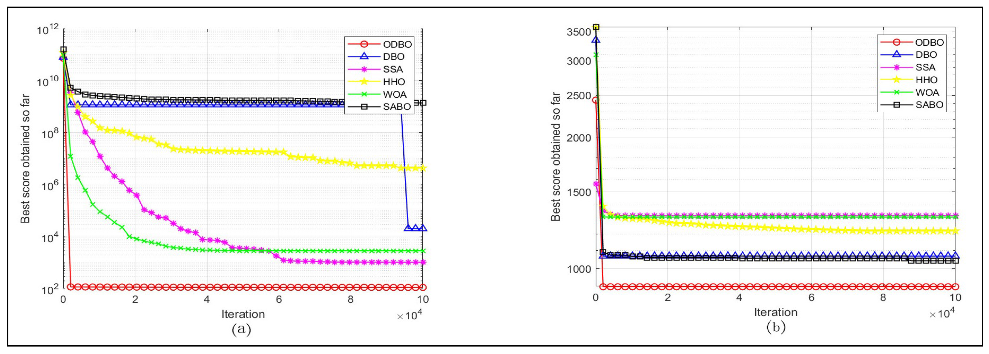
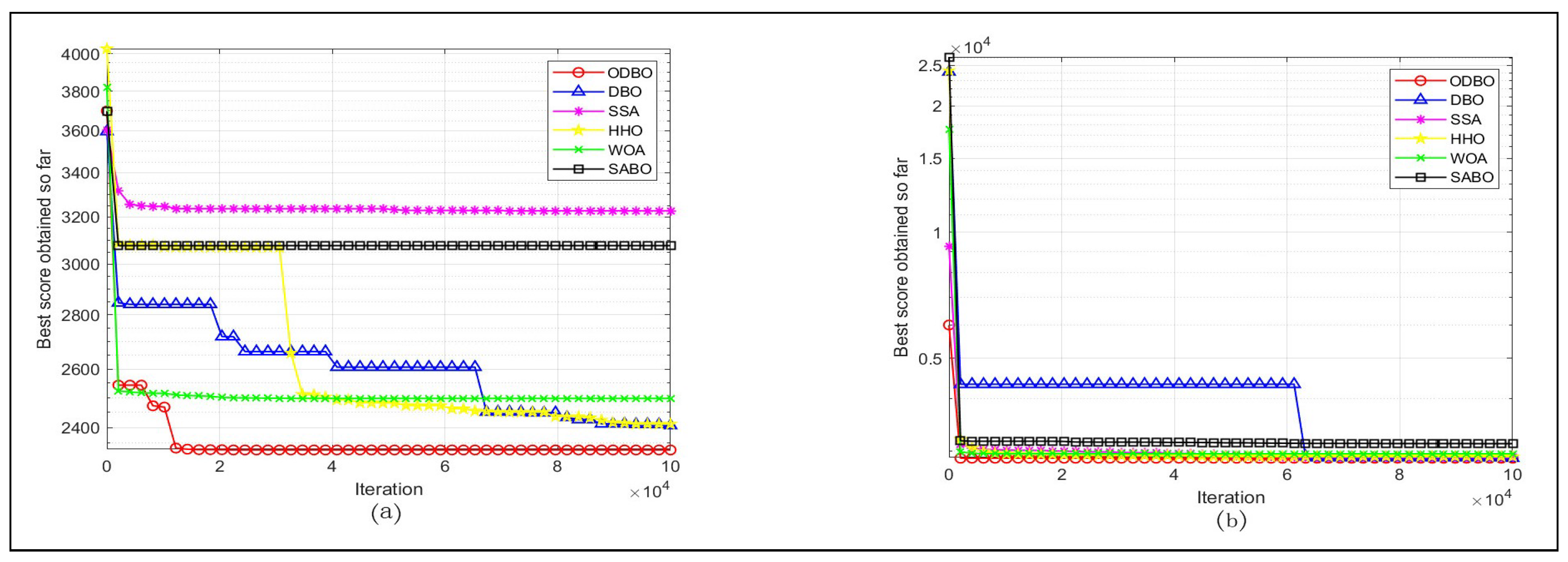
Figure 1 and
Figure 2 illustrate their operation on F1, F7, F20, and F25 of CEC2017, from which it can be seen that among the six algorithms, ODBO achieved the fastest convergence on F1, F7, and F25, and slightly slower than SABO on F20; however, ODBO always found the optimum in the shortest number of iterations, and the optimum was much smaller than the other five compared algorithms. It is also worth mentioning that ODBO converged fast in the preliminaries. Comparatively, DBO tends to require many iterations to converge and exhibits poor pre-exploration capabilities.
4.2.2. Accuracy
In this paper, the accuracy of ODBO is evaluated by comparing the effectiveness of ODBO and the five algorithms mentioned above on the CEC2017 test set.
Table A1 and
Table A2 (details in
Appendix A) are the experiment data of these six algorithms in the case of 10/30 dimensions. The mean, optima, worst, standard deviation, and median values obtained by these algorithms running on different functions in CEC2017 are listed in
Table A1 and
Table A2; their mean rankings on each test function are also given.
Based on the data in
Table A1 and
Table A2, ODBO performs poorly in 10 dimensions, but it tends to obtain better results than the DBO algorithm in single-peak and mixed-class test functions, especially when the results obtained by the DBO algorithm differ from the best results; In 30 dimensions, the ODBO algorithm runs significantly better than the DBO algorithm, performing excellently in the single-peak, simple multiple-peak, and mixed-class test functions, and slightly inferior to the DBO algorithm in the combined-class test functions.
In addition, based on the data in
Table A1 and
Table A2, it can be seen that ODBO is more suitable for solving higher-dimensional problems. In order to verify this property of ODBO,
Table 1 and
Table 2 give the experimental results of ODBO in 50 and 100 dimensions. The tables contain the mean and standard deviation as well as the ranking, and the PSO algorithm is added for comparison.
From the data in
Table A1 and
Table A2, it can be seen that the performance of ODBO in high-dimensional spaces presents a clear advantage over the other five swarm intelligence optimizations.
4.3. Friedman Test
In order to further rank the comparative performance of the algorithms, the Friedman test [
27] is used in this paper to examine the mean rankings of these six algorithms for 30 runs on each test function of the CEC2017 test set. The results of the test are shown in
Table 3, which lists the mean rankings of these six algorithms on CEC2017 for different dimensions along with their
p-values.
According to the data in
Table 3, the
p-value is less than 0.05 in all dimensions, so it can be concluded that all the compared algorithms perform significantly differently in the corresponding dimensions. Meanwhile, ODBO shows its superior performance in high numbers of dimensions, in that it is slightly inferior to DBO in 10 dimensions, but superior to DBO in 30, 50, and 100 dimensions, and the average ranking of ODBO in these four numbers of dimensions is much smaller than that of DBO.
4.4. Ablation Study
To assess the influence of the three algorithmic optimization components discussed in this study on the overall system, phase integration experiments were used, and the ablation of single units revealed their different contributions to the overall classification performance [
28]. In the ablation study, the dimensions were set to 10 and 30, and each algorithm was run 10 times on each test function.
Table A3 and
Table A4 (details in
Appendix A) illustrate the results of the ablation study in 10 and 30 dimensions, respectively. In the tables, the letters A, B, and C in front of DBO represent the three optimization strategies described in
Section 3, i.e., the letters in front of DBO indicate which optimization strategies are adopted.
From the results of the 10-dimensional ablation study, it can be seen that the vertical and horizontal crossover strategy (hereafter referred to as the B-strategy) negatively affects the algorithm’s average runtime effectiveness because the low-dimensional problems typically have a relatively small search space. When using the crossover strategy, the generated new solutions may be too similar, lacking sufficient diversity to explore the entire search space. However, the cat map and opposition-based learning strategy (hereinafter referred to as A-strategy) and the new rolling dung ball strategy (hereinafter referred to as C-strategy), which is mentioned above, enhance the algorithm’s average performance. However, it is worth mentioning that the B-strategy does not affect the ability of ODBO to find the optimal solution during its 30 runs on a test function.
From the results of the 30-dimensional ablation study, it can be seen that the A-strategy and C-strategy negatively affect the average running results of the algorithm, although the C-strategy is dominant among them, and it can also be seen that the combination of the B-strategy and the C-strategy does not have as big a negative impact on the algorithm as the combination of the A-strategy and the C-strategy. In addition, the B-strategy leads to a smaller optimal value of ODBO, but the combination of the A-strategy and B-strategy instead leads to a poor result of ODBO, and the negative impact of the A-strategy can be dispensed with by adding the C-strategy.
In summary, although the C-strategy makes the average running result of ODBO worse in both 10 or 30 dimensions, it can solve the conflict between the A-strategy and the B-strategy in 30 dimensions and obtain a better optimal value.
5. Engineering Applications
In order to verify the problem-solving ability of ODBO, in this section, the ODBO algorithm will be applied to two engineering applications: speed reducer design [
29] and compression spring design [
30], and the results of the runs will be compared with those of the five other algorithms.
5.1. Speed Reducer Design
The speed reducer design problem is an engineering design problem; the main objective of this design problem is to minimize the weight of the speed reducer while satisfying the constraints, and it can be presented as follows (
16).
where
to
are the seven design variables of the problem, which represent the face width (
b), the module of the teeth (
m), the number of gear teeth (
p), the length of the first axis between the bearings (
), the length of the second axis between the bearings (
), the diameter of the first axis (
), and the diameter of the second axis (
); there are also eleven constraint functions (
to
) for the problem.
Table 4 shows the results of ODBO and the five other algorithms running on the speed reducer problem, and it can be found that the ODBO has the smallest weight. Consequently, ODBO has a better performance than the other tested algorithms on such problems.
5.2. Compression Spring Design
The objective of compression spring design (CSD) is to minimize the spring’s mass
subject to certain constraints. The design issue consists of four inequality constraints, the minimum deflection, shear stress, oscillation frequency, and limit on the outer diameter, and three design variables, the average diameter of the spring coils(D), the diameter of the spring wires(d), and the number of active coils of the spring(N). The specific mathematical model is shown in (
17) below.
The constraint-processed mathematical model is solved using the six intelligent optimization algorithms described above.
Table 5 showed the detailed results of the comparative experiment.
From the data in the table, it can be seen that ODBO still obtains optimal results, indicating that ODBO performs well in this type of engineering problem.
6. Analysis and Discussion
In this paper, various properties of the proposed ODBO algorithm are clarified through the experiments described above. In addition, this paper compares the exploitation and exploration capabilities of ODBO and other algorithms on the CEC2017 test set in different dimensions and analyzes the reasons why ODBO exhibits these properties through ablation study. Meanwhile, to determine if ODBO has any value in engineering applications, this paper uses ODBO to solve two representative simple real-world problems, and the results show that ODBO performs well on both types of problems.
In our experiments, we found that ODBO converges very fast and can obtain better results than DBO with fewer iterations. In addition to this, ODBO can often perform better than DBO in high-dimensional spaces and achieve better results. However, ODBO is not stable enough in low-dimensional spaces, and can easily fall into local optima. In this paper, we conducted an ablation study and found that this is mainly the effect of the vertical and horizontal crossover strategy; however, the strategy is able to bring larger gains at high dimensions.
In conclusion, ODBO has excellent performance at high numbers of dimensions, but may not be stable enough to avoid falling into local optima at low numbers of dimensions. However, at the same time, it often has better performance than DBO in engineering problems. Therefore, in future research, the main goal will be to determine how to reduce the possibility of this algorithm falling into local optima in low-dimensional spaces.
7. Conclusions
In this paper, an enhanced DBO algorithm (ODBO) based on the cat mapping and opposition-based learning strategy, the osprey optimization algorithm, and the vertical and horizontal crossover strategy is proposed. The 29 test functions on the CEC2017 test set were used to test the performance of ODBO, including its convergence, population diversity, and accuracy. In addition, an ablation study showed the effects of the three enhancement strategies on the performance of ODBO. Moreover, ODBO is used to solve two real-world engineering design problems, and the results show the value of the ODBO algorithm in the real-world domain. Nevertheless, ODBO still has the defect of not being stable enough at low numbers of dimensions, which will be the focus of future work.
Author Contributions
Conceptualization, Y.S.; methodology, Y.S. and Q.C.; validation, H.K.; formal analysis, X.W.; investigation, X.S.; writing—original draft preparation, X.W.; writing—review and editing, X.W., H.K. and Q.C.; funding acquisition, H.K. and Y.S. All authors have read and agreed to the published version of the manuscript.
Funding
This research was supported by Open Foundation of Key Laboratory of Software Engineering of Yunnan Province (grant no. 2020SE308, 2020SE309).
Data Availability Statement
Data are contained within the article.
Conflicts of Interest
The authors declare no conflicts of interest.
Appendix A
Table A1.
Comparative Performance of ODBO (10 dimensions).
Table A1.
Comparative Performance of ODBO (10 dimensions).
| |
ODBO
|
DBO
|
HHO
|
SSA
|
WOA
|
SABO
|
|---|
| F1 | Mean | 861.14 | 5444.78 | 40,476.05 | 3783.35 | 3806.85 | 628,317.27 |
| | best | 100.05 | 132.53 | 6500.48 | 100.08 | 105.24 | 120,682.83 |
| | worst | 4328.76 | 12,740.83 | 101,725.39 | 12,735.19 | 12,748.67 | 2,648,334.93 |
| | std | 886.50 | 4267.76 | 28,512.90 | 3587.37 | 3820.37 | 589,833.00 |
| | median | 509.85 | 5261.17 | 29,826.27 | 2634.38 | 2368.60 | 373,737.10 |
| | rank | 1 | 4 | 5 | 2 | 3 | 6 |
| F3 | mean | 300.00 | 300.00 | 300.01 | 300.00 | 300.00 | 506.38 |
| | best | 300.00 | 300.00 | 300.00 | 300.00 | 300.00 | 304.60 |
| | worst | 300.00 | 300.00 | 300.05 | 300.00 | 300.00 | 3050.96 |
| | std | 0.00 | 0.00 | 0.01 | 0.00 | 0.00 | 496.99 |
| | median | 300.00 | 300.00 | 300.01 | 300.00 | 300.00 | 383.49 |
| | rank | 1 | 2 | 5 | 3 | 4 | 6 |
| F4 | Mean | 400.01 | 403.50 | 403.78 | 403.14 | 412.63 | 409.60 |
| | Min | 400.00 | 400.00 | 400.90 | 400.08 | 400.04 | 403.51 |
| | Max | 400.14 | 406.26 | 468.79 | 463.55 | 477.42 | 463.90 |
| | Std | 0.02 | 2.60 | 12.28 | 11.42 | 24.50 | 11.24 |
| | Median | 400.01 | 404.99 | 401.61 | 401.20 | 403.95 | 406.07 |
| | Rank | 1 | 3 | 4 | 2 | 6 | 5 |
| F5 | Mean | 526.62 | 520.40 | 526.40 | 563.87 | 540.37 | 529.35 |
| | Min | 506.96 | 507.96 | 510.97 | 527.86 | 508.95 | 511.63 |
| | Max | 555.72 | 537.81 | 556.79 | 622.35 | 575.62 | 548.15 |
| | Std | 11.52 | 8.57 | 9.39 | 25.19 | 17.04 | 9.15 |
| | Median | 525.16 | 518.90 | 523.90 | 558.70 | 542.29 | 528.97 |
| | Rank | 3 | 1 | 2 | 6 | 5 | 4 |
| F6 | Mean | 604.12 | 603.46 | 602.20 | 642.85 | 613.53 | 608.06 |
| | Min | 600.09 | 600.00 | 600.14 | 619.82 | 601.09 | 600.53 |
| | Max | 617.16 | 611.85 | 617.57 | 667.40 | 633.74 | 619.88 |
| | Std | 4.42 | 3.40 | 3.70 | 11.81 | 9.49 | 4.74 |
| | Median | 602.35 | 602.86 | 600.34 | 642.71 | 610.65 | 606.99 |
| | Rank | 3 | 2 | 1 | 6 | 5 | 4 |
| F7 | Mean | 745.92 | 741.03 | 744.47 | 812.33 | 755.43 | 736.79 |
| | Min | 720.48 | 715.62 | 718.07 | 765.65 | 730.71 | 724.32 |
| | Max | 786.50 | 798.82 | 764.08 | 830.41 | 773.79 | 759.18 |
| | Std | 17.16 | 17.05 | 11.32 | 13.79 | 12.28 | 7.14 |
| | Median | 744.17 | 738.59 | 746.46 | 814.89 | 756.53 | 735.46 |
| | Rank | 4 | 2 | 3 | 6 | 5 | 1 |
| F8 | Mean | 820.60 | 817.78 | 818.06 | 846.02 | 831.16 | 830.62 |
| | Min | 807.96 | 805.97 | 806.13 | 816.91 | 808.95 | 816.02 |
| | Max | 836.81 | 833.44 | 826.92 | 878.60 | 853.73 | 852.55 |
| | Std | 7.80 | 7.24 | 5.05 | 15.49 | 10.73 | 9.45 |
| | Median | 818.90 | 817.91 | 817.95 | 843.78 | 830.35 | 830.00 |
| | Rank | 3 | 1 | 2 | 6 | 5 | 4 |
| F9 | Mean | 924.38 | 910.84 | 923.91 | 1677.66 | 972.16 | 964.04 |
| | Min | 900.00 | 900.00 | 900.02 | 1187.55 | 900.03 | 901.07 |
| | Max | 1064.39 | 947.88 | 1127.72 | 2525.39 | 1358.49 | 1,075.95 |
| | Std | 39.72 | 13.27 | 64.19 | 251.66 | 96.71 | 52.63 |
| | Median | 908.63 | 904.29 | 900.05 | 1657.35 | 950.62 | 965.91 |
| | Rank | 3 | 1 | 2 | 6 | 5 | 4 |
| F10 | Mean | 1704.88 | 1586.03 | 1669.72 | 2354.35 | 1734.52 | 2302.70 |
| | Min | 1167.83 | 1140.21 | 1131.63 | 1734.92 | 1252.46 | 1780.95 |
| | Max | 2275.79 | 2036.14 | 2264.90 | 2870.28 | 2308.98 | 2734.63 |
| | Std | 296.46 | 238.19 | 251.12 | 314.22 | 273.90 | 253.44 |
| | Median | 1683.30 | 1566.08 | 1619.06 | 2373.73 | 1743.75 | 2334.62 |
| | Rank | 3 | 1 | 2 | 6 | 4 | 5 |
| F11 | Mean | 1119.75 | 1159.84 | 1122.48 | 1191.14 | 1146.89 | 1220.54 |
| | Min | 1102.98 | 1105.97 | 1106.07 | 1124.60 | 1109.35 | 1119.59 |
| | Max | 1152.51 | 1304.73 | 1150.89 | 1275.07 | 1285.44 | 1637.58 |
| | Std | 12.40 | 59.23 | 11.88 | 37.31 | 43.52 | 110.27 |
| | Median | 1118.27 | 1133.86 | 1121.31 | 1188.26 | 1131.68 | 1186.06 |
| | Rank | 1 | 4 | 2 | 5 | 3 | 6 |
| F12 | Mean | 12,025.18 | 291,570.06 | 27,271.93 | 34,271.89 | 337,534.23 | 441,392.69 |
| | Min | 2182.61 | 2004.27 | 5481.02 | 3259.06 | 3041.68 | 13,000.08 |
| | Max | 51,226.51 | 8,224,141.37 | 171,871.51 | 299,996.13 | 2,240,664.25 | 2,384,855.35 |
| | Std | 12,447.60 | 1,498,321.98 | 32,659.34 | 53,259.41 | 527,762.91 | 624,439.53 |
| | Median | 6903.58 | 11,354.48 | 17,100.72 | 20,087.28 | 95,705.48 | 81,846.10 |
| | Rank | 1 | 4 | 2 | 3 | 5 | 6 |
| F13 | Mean | 1479.79 | 3393.73 | 8484.82 | 10,157.15 | 14,266.43 | 9461.66 |
| | Min | 1317.18 | 1376.93 | 1761.12 | 1447.64 | 1708.89 | 3385.13 |
| | Max | 2086.40 | 20,703.52 | 22,709.62 | 32,764.56 | 41,113.18 | 16,638.99 |
| | Std | 192.39 | 3657.18 | 6929.22 | 10,128.33 | 11,510.28 | 3873.86 |
| | Median | 1387.53 | 2596.11 | 5603.41 | 4969.11 | 9589.88 | 8464.25 |
| | Rank | 1 | 2 | 3 | 5 | 6 | 4 |
| F14 | Mean | 1456.50 | 1454.09 | 1478.94 | 1668.14 | 1467.04 | 1474.31 |
| | Min | 1425.97 | 1424.28 | 1426.57 | 1430.75 | 1425.51 | 1446.92 |
| | Max | 1497.61 | 1509.60 | 1527.44 | 2351.36 | 1534.04 | 1517.52 |
| | Std | 22.59 | 22.62 | 22.66 | 208.98 | 28.90 | 19.58 |
| | Median | 1454.82 | 1448.94 | 1484.61 | 1625.57 | 1462.75 | 1471.19 |
| | Rank | 2 | 1 | 5 | 6 | 3 | 4 |
| F15 | Mean | 1565.53 | 1531.34 | 1556.91 | 1594.66 | 1610.31 | 2527.25 |
| | Min | 1502.16 | 1502.47 | 1504.71 | 1520.05 | 1521.04 | 1652.72 |
| | Max | 1700.86 | 1591.82 | 1638.13 | 1712.34 | 1732.42 | 4972.58 |
| | Std | 57.67 | 24.42 | 34.27 | 61.93 | 56.66 | 1046.91 |
| | Median | 1556.39 | 1526.23 | 1549.31 | 1585.65 | 1603.96 | 2076.77 |
| | Rank | 3 | 1 | 2 | 4 | 5 | 6 |
| F16 | Mean | 1692.58 | 1681.46 | 1800.78 | 1935.62 | 1724.60 | 1,957.67 |
| | Min | 1600.53 | 1601.04 | 1602.11 | 1719.58 | 1603.37 | 1760.97 |
| | Max | 1856.10 | 1871.14 | 2025.59 | 2281.63 | 1906.44 | 2115.76 |
| | Std | 89.03 | 93.62 | 128.89 | 160.13 | 113.11 | 98.82 |
| | Median | 1719.54 | 1639.54 | 1790.88 | 1925.56 | 1727.32 | 1981.33 |
| | Rank | 2 | 1 | 4 | 5 | 3 | 6 |
| F17 | Mean | 1743.94 | 1733.19 | 1752.57 | 1858.20 | 1758.65 | 1843.59 |
| | Min | 1716.13 | 1703.72 | 1712.16 | 1755.43 | 1725.99 | 1760.82 |
| | Max | 1803.42 | 1793.02 | 1803.44 | 2219.89 | 1806.99 | 1963.71 |
| | Std | 20.94 | 16.39 | 27.54 | 90.83 | 20.37 | 61.09 |
| | Median | 1740.68 | 1728.14 | 1744.75 | 1851.68 | 1756.79 | 1852.33 |
| | Rank | 2 | 1 | 3 | 6 | 4 | 5 |
| F18 | Mean | 1871.26 | 10,992.65 | 13,342.50 | 12,774.85 | 16,900.15 | 9657.25 |
| | Min | 1821.00 | 1822.02 | 2076.90 | 1898.89 | 3671.05 | 2325.72 |
| | Max | 1991.31 | 35,034.90 | 34,097.35 | 33,955.42 | 52,494.93 | 29,728.31 |
| | Std | 52.34 | 11,245.87 | 9588.49 | 10,846.68 | 11,418.80 | 6712.09 |
| | Median | 1849.23 | 6662.53 | 11,426.05 | 8541.78 | 14,087.94 | 8022.62 |
| | Rank | 1 | 3 | 5 | 4 | 6 | 2 |
| F19 | Mean | 1936.95 | 1955.05 | 1938.56 | 12,422.76 | 5013.29 | 3451.84 |
| | Min | 1902.07 | 1902.70 | 1906.50 | 2288.56 | 1956.26 | 1919.04 |
| | Max | 2042.10 | 2509.46 | 1991.69 | 33,397.64 | 15,866.25 | 9062.67 |
| | Std | 43.20 | 120.18 | 22.94 | 10,763.62 | 4204.40 | 1785.29 |
| | Median | 1918.68 | 1927.08 | 1934.85 | 6436.95 | 2618.05 | 2766.75 |
| | Rank | 1 | 3 | 2 | 6 | 5 | 4 |
| F20 | Mean | 2074.52 | 2042.49 | 2043.88 | 2219.32 | 2071.37 | 2191.59 |
| | Min | 2003.98 | 2013.02 | 2001.78 | 2076.85 | 2030.80 | 2067.30 |
| | Max | 2195.66 | 2093.94 | 2184.41 | 2406.45 | 2172.87 | 2282.30 |
| | Std | 59.23 | 20.95 | 37.73 | 84.32 | 31.12 | 48.01 |
| | Median | 2046.92 | 2039.09 | 2032.93 | 2207.82 | 2068.35 | 2199.72 |
| | Rank | 4 | 1 | 2 | 6 | 3 | 5 |
| F21 | Mean | 2254.78 | 2202.29 | 2304.57 | 2352.64 | 2232.56 | 2324.71 |
| | Min | 2200.00 | 2200.00 | 2200.01 | 2200.00 | 2200.00 | 2204.03 |
| | Max | 2335.68 | 2205.45 | 2385.27 | 2428.22 | 2354.41 | 2357.75 |
| | Std | 62.51 | 1.26 | 65.69 | 48.02 | 58.47 | 26.69 |
| | Median | 2203.55 | 2202.33 | 2333.04 | 2357.57 | 2201.14 | 2332.34 |
| | Rank | 3 | 1 | 4 | 6 | 2 | 5 |
| F22 | Mean | 2295.09 | 2304.35 | 2325.15 | 2739.69 | 2304.51 | 2308.34 |
| | Min | 2216.35 | 2300.29 | 2245.47 | 2328.01 | 2235.89 | 2304.20 |
| | Max | 2313.71 | 2318.14 | 2855.09 | 4593.87 | 2320.74 | 2330.83 |
| | Std | 22.77 | 4.18 | 101.60 | 630.33 | 22.75 | 5.34 |
| | Median | 2301.65 | 2302.62 | 2309.81 | 2417.78 | 2311.43 | 2307.03 |
| | Rank | 1 | 2 | 5 | 6 | 3 | 4 |
| F23 | Mean | 2632.03 | 2606.03 | 2637.79 | 2680.81 | 2631.48 | 2,632.12 |
| | Min | 2608.35 | 2302.80 | 2609.77 | 2629.62 | 2610.51 | 2617.92 |
| | Max | 2665.25 | 2665.55 | 2686.65 | 2806.75 | 2653.84 | 2666.23 |
| | Std | 13.87 | 82.48 | 19.05 | 39.47 | 12.09 | 10.84 |
| | Median | 2632.62 | 2627.12 | 2635.47 | 2677.01 | 2630.98 | 2628.64 |
| | Rank | 4 | 1 | 5 | 6 | 3 | 2 |
| F24 | Mean | 2726.53 | 2500.00 | 2750.36 | 2821.57 | 2761.03 | 2757.10 |
| | Min | 2500.00 | 2500.00 | 2500.14 | 2500.00 | 2500.01 | 2745.18 |
| | Max | 2849.01 | 2500.00 | 2906.04 | 2976.16 | 2803.80 | 2773.74 |
| | Std | 105.39 | 0.00 | 105.99 | 125.39 | 52.22 | 7.82 |
| | Median | 2760.07 | 2500.00 | 2778.96 | 2855.86 | 2765.93 | 2755.53 |
| | Rank | 2 | 1 | 3 | 6 | 5 | 4 |
| F25 | Mean | 2933.58 | 2936.30 | 2931.25 | 2960.40 | 2919.96 | 2940.31 |
| | Min | 2897.75 | 2897.94 | 2897.91 | 2899.58 | 2700.02 | 2898.67 |
| | Max | 2973.78 | 2971.23 | 2969.44 | 3130.62 | 2959.76 | 3028.90 |
| | Std | 25.95 | 25.20 | 23.35 | 55.39 | 63.78 | 29.27 |
| | Median | 2945.28 | 2947.83 | 2944.36 | 2957.35 | 2947.21 | 2944.52 |
| | Rank | 3 | 4 | 2 | 6 | 1 | 5 |
| F26 | Mean | 3117.23 | 3003.50 | 3039.84 | 3875.30 | 3223.73 | 3163.00 |
| | Min | 2600.00 | 2600.00 | 2600.87 | 2815.36 | 2600.01 | 2843.68 |
| | Max | 4181.83 | 3178.22 | 4115.67 | 4689.55 | 4306.42 | 4157.65 |
| | Std | 391.54 | 152.18 | 423.70 | 581.17 | 467.10 | 297.14 |
| | Median | 3020.69 | 3039.25 | 2900.45 | 4066.51 | 3044.67 | 3107.92 |
| | Rank | 3 | 1 | 2 | 6 | 5 | 4 |
| F27 | Mean | 3110.84 | 3095.65 | 3126.05 | 3228.58 | 3098.13 | 3103.28 |
| | Min | 3089.31 | 3089.31 | 3093.00 | 3107.98 | 3089.52 | 3092.25 |
| | Max | 3186.68 | 3104.64 | 3205.44 | 3432.86 | 3126.29 | 3119.37 |
| | Std | 28.11 | 3.26 | 33.46 | 72.45 | 7.74 | 6.95 |
| | Median | 3098.02 | 3095.29 | 3113.82 | 3216.50 | 3096.02 | 3102.61 |
| | Rank | 4 | 1 | 5 | 6 | 2 | 3 |
| F28 | Mean | 3431.22 | 3174.93 | 3313.95 | 3364.34 | 3228.41 | 3363.28 |
| | Min | 3100.00 | 3100.00 | 3100.45 | 3100.00 | 3100.00 | 3114.31 |
| | Max | 3749.37 | 3412.05 | 3444.13 | 3749.37 | 3411.82 | 3462.13 |
| | Std | 178.25 | 124.03 | 125.44 | 159.41 | 90.42 | 96.68 |
| | Median | 3411.89 | 3100.01 | 3383.75 | 3411.82 | 3215.91 | 3410.29 |
| | Rank | 6 | 1 | 3 | 5 | 2 | 4 |
| F29 | Mean | 3201.09 | 3167.38 | 3218.04 | 3407.74 | 3252.52 | 3249.19 |
| | Min | 3134.10 | 3131.57 | 3153.83 | 3186.52 | 3146.26 | 3157.45 |
| | Max | 3319.28 | 3227.94 | 3354.51 | 3728.68 | 3399.48 | 3437.59 |
| | Std | 49.67 | 23.70 | 43.22 | 148.99 | 65.77 | 73.56 |
| | Median | 3192.86 | 3164.17 | 3203.27 | 3365.28 | 3234.39 | 3231.25 |
| | Rank | 2 | 1 | 3 | 6 | 5 | 4 |
| F30 | Mean | 545,708.33 | 424,727.23 | 246,953.64 | 677,688.82 | 41,081.77 | 608,175.69 |
| | Min | 3456.77 | 3857.38 | 4897.28 | 4220.88 | 4705.30 | 6,084.85 |
| | Max | 4,737,611.44 | 1,760,900.98 | 1,721,162.03 | 4,757,519.66 | 820,578.06 | 3,161,260.04 |
| | Std | 1,240,300.95 | 561,347.23 | 457,703.17 | 1,184,340.55 | 147,733.26 | 811,466.62 |
| | Median | 3904.83 | 17,355.03 | 15,844.40 | 36,243.90 | 10,900.95 | 271,528.48 |
| | Rank | 4 | 3 | 2 | 6 | 1 | 5 |
| (#) | Best | 9 | 16 | 1 | 0 | 2 | 1 |
Table A2.
Comparative Performance of ODBO (30 dimensions).
Table A2.
Comparative Performance of ODBO (30 dimensions).
| |
ODBO
|
DBO
|
HHO
|
SSA
|
WOA
|
SABO
|
|---|
| F1 | Mean | 2771.75 | 11,635.85 | 4,371,879.00 | 3427.03 | 5697.96 | 2,676,267,000.00 |
| | Min | 100.09 | 109.70 | 2,912,012.00 | 119.10 | 475.80 | 962,481,400.00 |
| | Max | 15,773.86 | 20,941.77 | 5,802,485.00 | 16,700.23 | 17,346.32 | 7,070,487,000.00 |
| | Std | 4485.09 | 8168.68 | 804,167.80 | 3934.59 | 4418.48 | 1,328,230,000.00 |
| | Median | 948.23 | 7525.17 | 4,242,747.00 | 1962.36 | 5270.19 | 2,420,224,000.00 |
| | Rank | 1 | 4 | 5 | 2 | 3 | 6 |
| F3 | Mean | 300.00 | 300.05 | 319.34 | 1,014.77 | 40,608.46 | 14,635.05 |
| | Min | 300.00 | 300.00 | 312.67 | 336.10 | 10,503.43 | 6213.00 |
| | Max | 300.00 | 300.54 | 329.94 | 3433.24 | 92,169.43 | 39,660.44 |
| | Std | 0.00 | 0.13 | 4.52 | 722.14 | 20,243.21 | 6952.10 |
| | Median | 300.00 | 300.00 | 318.40 | 760.95 | 34,444.54 | 12,389.33 |
| | Rank | 1 | 2 | 3 | 4 | 6 | 5 |
| F4 | Mean | 438.77 | 483.86 | 500.96 | 485.12 | 496.42 | 886.27 |
| | Min | 400.00 | 400.99 | 407.17 | 402.89 | 459.60 | 569.57 |
| | Max | 526.32 | 593.12 | 543.73 | 521.65 | 522.64 | 2,031.66 |
| | Std | 47.41 | 39.75 | 26.08 | 26.63 | 17.90 | 342.79 |
| | Median | 404.14 | 489.22 | 511.77 | 482.10 | 491.63 | 723.88 |
| | Rank | 1 | 2 | 5 | 3 | 4 | 6 |
| F5 | Mean | 667.19 | 680.84 | 698.48 | 798.40 | 787.91 | 738.04 |
| | Min | 592.53 | 552.73 | 627.56 | 744.76 | 719.65 | 689.06 |
| | Max | 751.72 | 773.66 | 763.59 | 876.24 | 891.01 | 770.92 |
| | Std | 40.77 | 58.31 | 30.27 | 24.93 | 41.71 | 25.46 |
| | Median | 667.65 | 687.85 | 696.95 | 804.45 | 784.06 | 745.59 |
| | Rank | 1 | 2 | 3 | 6 | 5 | 4 |
| F6 | Mean | 630.17 | 627.65 | 650.39 | 670.50 | 664.99 | 646.46 |
| | Min | 609.37 | 612.52 | 624.05 | 650.62 | 649.44 | 633.90 |
| | Max | 659.17 | 658.81 | 662.33 | 694.96 | 685.62 | 663.22 |
| | Std | 9.70 | 14.07 | 9.91 | 9.24 | 9.30 | 7.87 |
| | Median | 629.58 | 621.32 | 650.78 | 669.63 | 663.94 | 646.03 |
| | Rank | 2 | 1 | 4 | 6 | 5 | 3 |
| F7 | Mean | 1011.54 | 949.42 | 1125.31 | 1326.63 | 1216.49 | 1047.28 |
| | Min | 901.60 | 832.21 | 994.32 | 1,213.47 | 1060.55 | 960.69 |
| | Max | 1176.78 | 1162.40 | 1,277.88 | 1363.14 | 1348.47 | 1206.57 |
| | Std | 65.08 | 80.03 | 65.40 | 26.29 | 78.94 | 58.10 |
| | Median | 1014.19 | 930.76 | 1122.01 | 1332.70 | 1228.09 | 1028.59 |
| | Rank | 2 | 1 | 4 | 6 | 5 | 3 |
| F8 | Mean | 936.78 | 968.03 | 943.30 | 994.51 | 993.97 | 1002.54 |
| | Min | 891.54 | 890.74 | 901.65 | 947.25 | 923.37 | 947.15 |
| | Max | 984.22 | 1047.39 | 994.00 | 1062.67 | 1111.42 | 1146.73 |
| | Std | 24.43 | 42.59 | 24.62 | 24.74 | 41.42 | 41.35 |
| | Median | 934.82 | 967.10 | 943.12 | 997.00 | 983.57 | 993.87 |
| | Rank | 1 | 3 | 2 | 5 | 4 | 6 |
| F9 | Mean | 3310.71 | 3653.03 | 5286.88 | 5393.36 | 7118.71 | 3866.76 |
| | Min | 1478.68 | 1553.79 | 3847.58 | 5005.37 | 4377.41 | 2428.71 |
| | Max | 4864.14 | 6849.88 | 6345.13 | 5562.35 | 14,223.28 | 5561.60 |
| | Std | 806.33 | 1426.83 | 556.14 | 110.19 | 2587.51 | 840.97 |
| | Median | 3225.69 | 3467.74 | 5437.57 | 5418.92 | 6316.18 | 3637.72 |
| | Rank | 1 | 2 | 4 | 5 | 6 | 3 |
| F10 | Mean | 4801.83 | 5336.12 | 4932.59 | 5906.22 | 5784.99 | 7901.41 |
| | Min | 3582.19 | 3516.54 | 3744.15 | 4395.73 | 4287.98 | 7047.10 |
| | Max | 5860.84 | 7232.40 | 6220.44 | 7327.28 | 7347.55 | 8710.53 |
| | Std | 642.24 | 870.19 | 598.91 | 719.45 | 682.35 | 403.82 |
| | Median | 4793.31 | 5264.63 | 4915.07 | 5802.38 | 5657.54 | 7914.76 |
| | Rank | 1 | 3 | 2 | 5 | 4 | 6 |
| F11 | Mean | 1240.04 | 1340.64 | 1233.23 | 1239.76 | 1247.07 | 1765.20 |
| | Min | 1141.39 | 1202.62 | 1153.27 | 1147.45 | 1126.21 | 1411.17 |
| | Max | 1385.22 | 1624.59 | 1309.68 | 1352.00 | 1339.45 | 2711.11 |
| | Std | 70.95 | 93.75 | 43.32 | 54.74 | 54.06 | 295.16 |
| | Median | 1213.42 | 1329.28 | 1233.24 | 1231.86 | 1254.00 | 1654.91 |
| | Rank | 3 | 5 | 1 | 2 | 4 | 6 |
| F12 | Mean | 29,122.47 | 3,384,297.76 | 3,847,104.82 | 5,661,165.88 | 8,550,797.51 | 113,420,679.40 |
| | Min | 9,928.68 | 89,218.57 | 1,170,668.44 | 315,175.00 | 789,420.11 | 6,013,554.94 |
| | Max | 94,490.62 | 12,520,448.57 | 8,098,426.82 | 25,941,955.51 | 26,597,474.74 | 423,718,099.40 |
| | Std | 18,832.59 | 3,819,269.87 | 1,978,848.97 | 5,698,037.83 | 7,484,040.93 | 117,412,400.00 |
| | Median | 23,449.23 | 2,018,825.72 | 3,531,145.73 | 4,168,797.06 | 6,503,727.75 | 52,588,936.52 |
| | Rank | 1 | 2 | 3 | 4 | 5 | 6 |
| F13 | Mean | 12,339.57 | 181,894.63 | 173,424.77 | 24,193.31 | 154,740.68 | 344,482.35 |
| | Min | 1798.87 | 14,584.93 | 44,058.17 | 6161.05 | 27,450.42 | 170,198.80 |
| | Max | 69,573.79 | 1,271,364.69 | 499,035.93 | 61,635.58 | 461,808.70 | 579,331.84 |
| | Std | 13,662.73 | 254,316.80 | 104,361.82 | 13,778.98 | 101,385.26 | 112,739.55 |
| | Median | 7264.54 | 107,813.02 | 156,024.33 | 22,018.84 | 127,889.01 | 334,604.30 |
| | Rank | 1 | 5 | 4 | 2 | 3 | 6 |
| F14 | Mean | 2651.49 | 15,446.98 | 13,565.08 | 76,981.93 | 84,598.10 | 91,899.11 |
| | Min | 1507.86 | 2256.03 | 1806.35 | 5467.63 | 6689.92 | 3033.09 |
| | Max | 6414.55 | 52,301.46 | 35,043.05 | 264,462.28 | 563,803.34 | 571,543.17 |
| | Std | 1021.70 | 15,501.36 | 8443.13 | 66,638.53 | 111,901.29 | 141,545.29 |
| | Median | 2528.26 | 9540.77 | 12,092.64 | 62,700.37 | 51,235.78 | 35,639.14 |
| | Rank | 1 | 3 | 2 | 4 | 5 | 6 |
| F15 | Mean | 9786.54 | 83,970.17 | 35,941.19 | 9906.68 | 61,109.53 | 29,144.49 |
| | Min | 1716.55 | 6037.35 | 13,524.10 | 2416.16 | 4737.53 | 13,100.64 |
| | Max | 32,667.20 | 344,115.28 | 93,874.80 | 35,168.41 | 260,789.99 | 63,240.47 |
| | Std | 8584.88 | 81,059.62 | 19,829.46 | 10,153.94 | 55,336.10 | 11,731.51 |
| | Median | 5533.12 | 60,364.14 | 31,231.28 | 6016.48 | 44,674.30 | 25,835.97 |
| | Rank | 1 | 6 | 4 | 2 | 5 | 3 |
| F16 | Mean | 2753.04 | 2605.29 | 2894.08 | 3408.24 | 2847.48 | 3448.36 |
| | Min | 2261.20 | 2000.84 | 2181.71 | 2745.70 | 2170.51 | 2918.17 |
| | Max | 3420.34 | 3047.00 | 4084.77 | 4250.03 | 3805.59 | 4203.16 |
| | Std | 264.76 | 304.88 | 414.97 | 343.83 | 418.86 | 317.31 |
| | Median | 2732.65 | 2621.15 | 2858.14 | 3370.84 | 2835.01 | 3469.85 |
| | Rank | 2 | 1 | 4 | 5 | 3 | 6 |
| F17 | Mean | 2351.85 | 2127.37 | 2381.57 | 3189.46 | 2343.69 | 2650.66 |
| | Min | 1811.27 | 1875.15 | 1955.42 | 2246.18 | 1936.44 | 2224.69 |
| | Max | 2973.01 | 2488.78 | 2726.99 | 4292.47 | 2800.31 | 3303.33 |
| | Std | 284.85 | 167.62 | 230.63 | 527.85 | 242.01 | 261.23 |
| | Median | 2367.11 | 2101.54 | 2399.86 | 3164.02 | 2353.85 | 2658.58 |
| | Rank | 3 | 1 | 4 | 6 | 2 | 5 |
| F18 | Mean | 35,778.21 | 291,473.42 | 129,489.13 | 384,199.29 | 690,768.13 | 515,284.99 |
| | Min | 3170.36 | 4667.21 | 31,004.69 | 40,077.88 | 49,251.86 | 57,408.70 |
| | Max | 375,683.29 | 1,290,669.58 | 401,161.76 | 1,230,598.43 | 2,811,412.15 | 2,202,196.77 |
| | Std | 67,261.65 | 300,996.47 | 97,490.67 | 361,904.83 | 866,096.88 | 540,874.95 |
| | Median | 18,811.40 | 183,162.66 | 93,559.03 | 183,422.67 | 314,892.71 | 322,143.21 |
| | Rank | 1 | 3 | 2 | 4 | 6 | 5 |
| F19 | Mean | 10,223.97 | 38,337.44 | 68,516.68 | 12,854.47 | 524,317.55 | 283,672.81 |
| | Min | 2166.89 | 2260.82 | 11,537.50 | 3900.83 | 9461.23 | 13,490.70 |
| | Max | 55,848.86 | 132,218.97 | 139,420.80 | 119,527.49 | 1,835,282.43 | 1,521,871.20 |
| | Std | 10,498.32 | 31,401.12 | 34,769.09 | 20,863.43 | 490,892.89 | 316,597.96 |
| | Median | 7,054.74 | 34,951.58 | 61,939.13 | 7515.31 | 354,591.78 | 154,389.05 |
| | Rank | 1 | 3 | 4 | 2 | 6 | 5 |
| F20 | Mean | 2451.86 | 2346.89 | 2601.62 | 2921.55 | 2635.37 | 2847.06 |
| | Min | 2218.45 | 2164.67 | 2209.25 | 2382.26 | 2309.89 | 2506.64 |
| | Max | 3070.22 | 2592.71 | 3039.40 | 3316.86 | 3044.34 | 3170.43 |
| | Std | 178.53 | 97.33 | 215.26 | 210.96 | 172.11 | 167.07 |
| | Median | 2422.43 | 2318.70 | 2582.27 | 2902.71 | 2647.07 | 2848.80 |
| | Rank | 2 | 1 | 3 | 6 | 4 | 5 |
| F21 | Mean | 2439.13 | 2407.86 | 2508.25 | 2662.38 | 2580.32 | 2531.19 |
| | Min | 2365.53 | 2204.54 | 2463.04 | 2513.22 | 2426.58 | 2477.76 |
| | Max | 2535.44 | 2545.04 | 2578.40 | 2818.00 | 2735.73 | 2583.34 |
| | Std | 38.79 | 105.48 | 33.11 | 69.87 | 73.98 | 31.92 |
| | Median | 2436.88 | 2432.95 | 2503.61 | 2650.65 | 2567.66 | 2532.05 |
| | Rank | 2 | 1 | 3 | 6 | 5 | 4 |
| F22 | Mean | 4056.96 | 2572.08 | 5834.19 | 7616.40 | 5985.34 | 3279.45 |
| | Min | 2300.00 | 2300.00 | 2315.31 | 6497.77 | 2300.65 | 2492.08 |
| | Max | 8060.44 | 5526.70 | 7809.77 | 8663.68 | 9072.92 | 6281.43 |
| | Std | 2109.85 | 758.54 | 2034.68 | 571.77 | 2183.23 | 817.58 |
| | Median | 2304.24 | 2304.02 | 6590.17 | 7712.35 | 6668.18 | 3024.07 |
| | Rank | 3 | 1 | 4 | 6 | 5 | 2 |
| F23 | Mean | 2895.75 | 2867.25 | 2996.35 | 3309.60 | 3032.05 | 3041.48 |
| | Min | 2768.01 | 2778.38 | 2819.62 | 2989.18 | 2842.35 | 2941.81 |
| | Max | 3058.69 | 3083.73 | 3174.49 | 3659.24 | 3192.41 | 3174.86 |
| | Std | 74.41 | 66.04 | 75.86 | 154.07 | 100.08 | 66.69 |
| | Median | 2898.67 | 2861.51 | 2987.08 | 3285.40 | 3028.83 | 3035.92 |
| | Rank | 2 | 1 | 3 | 6 | 4 | 5 |
| F24 | Mean | 3101.33 | 3019.60 | 3376.15 | 3490.92 | 3168.84 | 3161.54 |
| | Min | 2930.37 | 2905.82 | 3121.07 | 3182.80 | 3008.18 | 3062.31 |
| | Max | 3398.20 | 3208.45 | 3598.57 | 3772.34 | 3354.65 | 3261.16 |
| | Std | 110.81 | 79.26 | 115.82 | 136.67 | 90.65 | 52.25 |
| | Median | 3086.85 | 3008.08 | 3405.95 | 3500.81 | 3173.93 | 3164.64 |
| | Rank | 2 | 1 | 5 | 6 | 4 | 3 |
| F25 | Mean | 2897.44 | 2901.04 | 2897.66 | 2922.64 | 2927.59 | 3111.44 |
| | Min | 2883.66 | 2883.67 | 2883.99 | 2885.62 | 2885.93 | 3000.35 |
| | Max | 2938.11 | 2951.13 | 2938.17 | 2983.72 | 2989.19 | 3512.93 |
| | Std | 15.37 | 20.23 | 16.08 | 27.22 | 29.25 | 117.98 |
| | Median | 2890.09 | 2889.76 | 2890.87 | 2915.66 | 2930.90 | 3090.08 |
| | Rank | 1 | 3 | 2 | 4 | 5 | 6 |
| F26 | Mean | 5753.94 | 4800.56 | 6125.07 | 8998.23 | 6869.82 | 7087.81 |
| | Min | 2900.00 | 2900.00 | 2909.48 | 5591.69 | 2800.92 | 4132.38 |
| | Max | 8038.44 | 6307.60 | 7939.56 | 11,354.93 | 9398.34 | 9444.73 |
| | Std | 998.25 | 998.82 | 1429.69 | 1174.81 | 1454.94 | 1423.83 |
| | Median | 5726.45 | 5105.00 | 6479.29 | 9023.17 | 7057.25 | 7399.49 |
| | Rank | 2 | 1 | 3 | 6 | 4 | 5 |
| F27 | Mean | 3293.59 | 3280.04 | 3267.14 | 3765.24 | 3299.38 | 3354.36 |
| | Min | 3222.69 | 3220.95 | 3223.16 | 3384.83 | 3223.86 | 3222.30 |
| | Max | 3558.71 | 3488.27 | 3360.39 | 5022.88 | 3566.25 | 3557.30 |
| | Std | 75.32 | 53.09 | 29.19 | 401.24 | 80.13 | 92.45 |
| | Median | 3274.53 | 3260.29 | 3263.18 | 3649.05 | 3279.40 | 3330.63 |
| | Rank | 3 | 2 | 1 | 6 | 4 | 5 |
| F28 | Mean | 3143.77 | 3248.30 | 3221.18 | 3231.48 | 3230.33 | 3594.46 |
| | Min | 3100.00 | 3135.32 | 3103.16 | 3199.95 | 3197.28 | 3375.67 |
| | Max | 3261.85 | 3376.34 | 3261.47 | 3269.70 | 3386.82 | 4119.58 |
| | Std | 64.65 | 42.44 | 31.19 | 23.60 | 36.55 | 176.17 |
| | Median | 3100.00 | 3251.68 | 3215.40 | 3227.23 | 3216.37 | 3541.44 |
| | Rank | 1 | 5 | 2 | 4 | 3 | 6 |
| F29 | Mean | 4065.12 | 4078.29 | 4052.41 | 5437.20 | 4310.03 | 4847.60 |
| | Min | 3670.37 | 3494.83 | 3642.43 | 4529.30 | 3784.78 | 4162.51 |
| | Max | 4777.19 | 4730.23 | 4643.55 | 7622.84 | 5198.04 | 5700.05 |
| | Std | 277.98 | 282.19 | 279.26 | 706.42 | 339.27 | 400.63 |
| | Median | 4056.40 | 4080.80 | 3994.15 | 5250.17 | 4249.67 | 4776.13 |
| | Rank | 2 | 3 | 1 | 6 | 4 | 5 |
| F30 | Mean | 72,623.55 | 935,070.58 | 339,804.14 | 165,131.41 | 3,794,006.15 | 4,203,038.93 |
| | Min | 5083.58 | 20,905.81 | 86,196.28 | 20,149.37 | 631,665.09 | 364,881.16 |
| | Max | 813,472.17 | 9,511,088.12 | 898,320.04 | 561,520.96 | 9,022,587.27 | 17,101,108.31 |
| | Std | 169,646.10 | 2,090,365.15 | 170,334.59 | 125,268.35 | 2,542,204.35 | 3,758,415.54 |
| | Median | 14,998.65 | 178,006.07 | 315,621.98 | 132,065.74 | 2,834,691.40 | 3,552,881.51 |
| | Rank | 1 | 6 | 3 | 2 | 4 | 5 |
| (#) | Best | 16 | 10 | 3 | 0 | 0 | 0 |
Table A3.
Ablation Study (10 dimensions).
Table A3.
Ablation Study (10 dimensions).
| | ODBO | BCDBO | ACDBO | ABDBO | ADBO | BDBO | CDBO |
|---|
| F1 | Mean | 821.00 | 1203.36 | 174,505,435.40 | 1259.87 | 3795.27 | 1979.72 | 753,243,666.40 |
| | Min | 101.07 | 118.45 | 759.66 | 147.24 | 112.98 | 217.04 | 281.37 |
| | Max | 2313.31 | 5469.57 | 1,674,961,782.00 | 3133.82 | 5631.98 | 5214.69 | 3,086,914,054.00 |
| | Std | 871.17 | 1621.11 | 527,666,100.90 | 1146.07 | 2123.92 | 1812.00 | 1,058,676,731.00 |
| | Median | 429.56 | 659.99 | 4950.20 | 709.46 | 4560.64 | 1599.95 | 70,058,020.80 |
| F3 | Mean | 300.00 | 300.00 | 856.07 | 300.00 | 300.00 | 300.00 | 1051.36 |
| | Min | 300.00 | 300.00 | 300.00 | 300.00 | 300.00 | 300.00 | 300.00 |
| | Max | 300.00 | 300.00 | 3080.33 | 300.00 | 300.00 | 300.00 | 4553.84 |
| | Std | 0.00 | 0.00 | 1172.29 | 0.00 | 0.00 | 0.00 | 1404.86 |
| | Median | 300.00 | 300.00 | 300.00 | 300.00 | 300.00 | 300.00 | 300.00 |
| F4 | Mean | 400.01 | 400.02 | 466.91 | 400.00 | 412.93 | 400.00 | 477.22 |
| | Min | 400.00 | 400.00 | 400.00 | 400.00 | 400.00 | 400.00 | 400.00 |
| | Max | 400.04 | 400.15 | 637.46 | 400.00 | 455.62 | 400.00 | 698.10 |
| | Std | 0.01 | 0.04 | 80.30 | 0.00 | 22.64 | 0.00 | 97.39 |
| | Median | 400.01 | 400.01 | 439.42 | 400.00 | 402.96 | 400.00 | 445.03 |
| F5 | Mean | 529.10 | 532.20 | 533.10 | 523.42 | 523.57 | 521.76 | 538.42 |
| | Min | 515.92 | 515.92 | 509.95 | 508.95 | 506.96 | 508.95 | 508.95 |
| | Max | 541.79 | 571.64 | 553.28 | 534.96 | 537.73 | 533.04 | 563.88 |
| | Std | 7.75 | 15.41 | 13.84 | 8.57 | 9.94 | 9.58 | 17.71 |
| | Median | 529.35 | 527.86 | 533.98 | 525.37 | 526.86 | 521.39 | 540.00 |
| F6 | Mean | 603.23 | 602.97 | 605.02 | 603.49 | 602.31 | 601.28 | 613.62 |
| | Min | 600.01 | 600.20 | 600.19 | 600.09 | 600.13 | 600.06 | 600.63 |
| | Max | 610.47 | 608.47 | 608.75 | 606.64 | 605.92 | 605.01 | 640.70 |
| | Std | 3.18 | 2.83 | 2.59 | 2.46 | 2.28 | 1.52 | 12.01 |
| | Median | 602.29 | 602.12 | 604.44 | 603.59 | 601.33 | 600.77 | 609.59 |
| F7 | Mean | 740.83 | 743.83 | 742.50 | 736.87 | 738.02 | 745.39 | 743.34 |
| | Min | 727.66 | 730.00 | 727.91 | 725.91 | 717.98 | 729.12 | 717.75 |
| | Max | 748.45 | 764.70 | 803.74 | 751.20 | 766.61 | 772.80 | 770.78 |
| | Std | 5.89 | 11.91 | 22.40 | 9.27 | 14.93 | 15.80 | 17.26 |
| | Median | 741.36 | 745.13 | 733.86 | 735.19 | 739.70 | 739.86 | 744.14 |
| F8 | Mean | 820.20 | 817.51 | 824.28 | 819.10 | 821.24 | 816.89 | 824.56 |
| | Min | 813.93 | 810.94 | 811.94 | 808.95 | 809.06 | 810.94 | 807.96 |
| | Max | 827.86 | 824.87 | 836.84 | 830.84 | 832.21 | 824.87 | 836.52 |
| | Std | 4.92 | 4.79 | 8.72 | 8.03 | 8.03 | 4.80 | 9.52 |
| | Median | 821.89 | 815.92 | 828.67 | 819.90 | 821.97 | 817.41 | 826.40 |
| F9 | Mean | 948.80 | 910.06 | 1032.83 | 928.11 | 907.38 | 916.49 | 1006.21 |
| | Min | 900.18 | 901.09 | 902.27 | 900.45 | 900.09 | 900.45 | 905.18 |
| | Max | 1173.73 | 927.57 | 1125.03 | 972.31 | 920.69 | 952.35 | 1458.45 |
| | Std | 85.89 | 8.18 | 84.64 | 23.09 | 7.68 | 18.95 | 169.48 |
| | Median | 906.27 | 908.27 | 1063.38 | 929.11 | 903.86 | 908.68 | 926.57 |
| F10 | Mean | 1547.30 | 1700.69 | 1577.30 | 1570.84 | 1565.35 | 1623.62 | 1595.17 |
| | Min | 1015.18 | 1133.62 | 1155.94 | 1266.84 | 1018.60 | 1138.55 | 1246.19 |
| | Max | 2010.70 | 2315.13 | 1954.54 | 1978.38 | 2123.74 | 2138.55 | 2113.82 |
| | Std | 341.36 | 383.72 | 224.33 | 203.84 | 312.37 | 327.69 | 262.10 |
| | Median | 1580.15 | 1757.73 | 1578.03 | 1556.03 | 1641.43 | 1624.34 | 1591.14 |
| F11 | Mean | 1122.62 | 1116.19 | 1291.16 | 1131.16 | 1146.48 | 1119.32 | 1319.23 |
| | Min | 1105.97 | 1102.98 | 1125.99 | 1105.97 | 1107.96 | 1105.97 | 1110.07 |
| | Max | 1138.80 | 1133.83 | 1613.16 | 1164.67 | 1219.42 | 1154.72 | 1992.43 |
| | Std | 12.33 | 9.79 | 158.24 | 17.49 | 32.50 | 15.88 | 307.12 |
| | Median | 1123.24 | 1113.79 | 1260.38 | 1129.85 | 1136.82 | 1114.92 | 1182.00 |
| F12 | Mean | 11,640.11 | 8194.98 | 6,406,249.85 | 13,476.52 | 23,647.90 | 14,365.94 | 512,243.69 |
| | Min | 1415.59 | 1714.53 | 2926.11 | 2191.74 | 3759.59 | 2571.23 | 2530.23 |
| | Max | 32,876.82 | 20,841.51 | 23,826,741.10 | 47,044.21 | 147,259.78 | 52,385.51 | 4,950,892.56 |
| | Std | 10,205.32 | 7548.98 | 9,770,450.16 | 14,853.11 | 43,776.39 | 14,841.62 | 1,559,673.78 |
| | Median | 9422.62 | 5039.15 | 7391.09 | 6229.28 | 9503.22 | 10,953.25 | 15,937.72 |
| F13 | Mean | 1497.52 | 1488.72 | 7252.56 | 1477.25 | 5511.74 | 1652.80 | 11,817.51 |
| | Min | 1316.41 | 1328.26 | 1390.59 | 1322.51 | 1480.89 | 1321.13 | 1534.34 |
| | Max | 2059.89 | 1859.48 | 32,913.93 | 1737.96 | 33,008.66 | 2145.97 | 39,551.22 |
| | Std | 225.07 | 166.74 | 10,722.71 | 157.07 | 9710.73 | 284.12 | 14,438.77 |
| | Median | 1407.76 | 1477.16 | 2275.70 | 1416.96 | 2324.46 | 1623.99 | 2581.83 |
| F14 | Mean | 1446.72 | 1469.10 | 1467.98 | 1445.09 | 1462.10 | 1440.60 | 1466.47 |
| | Min | 1415.00 | 1410.95 | 1427.08 | 1405.27 | 1440.79 | 1413.04 | 1431.94 |
| | Max | 1469.75 | 1552.87 | 1518.14 | 1480.98 | 1495.85 | 1471.15 | 1524.42 |
| | Std | 17.91 | 38.52 | 31.32 | 21.07 | 20.24 | 16.75 | 32.36 |
| | Median | 1452.83 | 1463.30 | 1460.06 | 1441.56 | 1457.77 | 1440.55 | 1455.59 |
| F15 | Mean | 1546.53 | 1535.64 | 1581.91 | 1520.45 | 1535.60 | 1536.74 | 2305.71 |
| | Min | 1504.58 | 1503.00 | 1509.31 | 1505.45 | 1504.94 | 1504.14 | 1507.74 |
| | Max | 1601.64 | 1628.37 | 1670.91 | 1546.27 | 1610.87 | 1590.34 | 8744.54 |
| | Std | 36.19 | 39.12 | 48.23 | 13.70 | 31.47 | 33.25 | 2263.18 |
| | Median | 1535.63 | 1529.21 | 1572.08 | 1516.10 | 1527.05 | 1523.25 | 1594.66 |
| F16 | Mean | 1757.16 | 1782.85 | 1720.97 | 1668.96 | 1663.69 | 1724.04 | 1794.79 |
| | Min | 1601.91 | 1601.52 | 1601.98 | 1600.70 | 1601.37 | 1601.31 | 1600.78 |
| | Max | 1998.06 | 1973.79 | 1884.08 | 1735.21 | 1848.59 | 1893.18 | 1992.01 |
| | Std | 125.95 | 125.24 | 102.77 | 63.82 | 87.58 | 112.88 | 125.88 |
| | Median | 1732.01 | 1786.85 | 1687.93 | 1679.85 | 1611.33 | 1727.49 | 1775.72 |
| F17 | Mean | 1733.51 | 1729.26 | 1756.60 | 1728.61 | 1731.98 | 1736.88 | 1760.59 |
| | Min | 1709.57 | 1705.58 | 1702.47 | 1705.22 | 1702.67 | 1716.71 | 1723.10 |
| | Max | 1766.08 | 1757.90 | 1820.08 | 1750.79 | 1,744.95 | 1750.34 | 1876.85 |
| | Std | 17.20 | 16.18 | 42.55 | 14.21 | 13.42 | 10.15 | 44.47 |
| | Median | 1733.13 | 1727.56 | 1754.82 | 1724.56 | 1735.21 | 1739.61 | 1748.88 |
| F18 | Mean | 3980.85 | 1876.74 | 11,525.76 | 1868.24 | 3456.31 | 1847.47 | 14,643.55 |
| | Min | 1822.06 | 1828.43 | 1864.78 | 1822.27 | 1830.52 | 1821.40 | 1874.17 |
| | Max | 22,637.10 | 1965.70 | 55,272.42 | 2005.84 | 12,807.91 | 1923.48 | 35,085.85 |
| | Std | 6556.02 | 53.28 | 18,495.36 | 64.21 | 3554.17 | 30.07 | 15,290.45 |
| | Median | 1874.56 | 1859.69 | 2118.52 | 1845.82 | 1939.74 | 1837.22 | 5783.31 |
| F19 | Mean | 1933.73 | 1957.09 | 2007.67 | 1913.49 | 1930.67 | 1924.10 | 8258.55 |
| | Min | 1904.05 | 1904.52 | 1906.46 | 1905.97 | 1902.33 | 1901.44 | 1902.01 |
| | Max | 2041.38 | 2047.25 | 2699.18 | 1929.82 | 2040.03 | 2035.30 | 33,102.17 |
| | Std | 44.88 | 51.19 | 245.98 | 7.38 | 40.03 | 40.29 | 13,087.73 |
| | Median | 1911.88 | 1931.47 | 1923.54 | 1911.68 | 1916.51 | 1910.31 | 1964.48 |
| F20 | Mean | 2087.71 | 2079.28 | 2057.92 | 2037.59 | 2034.50 | 2049.47 | 2058.65 |
| | Min | 2001.99 | 2010.26 | 2021.33 | 2021.62 | 2009.09 | 2009.95 | 2023.22 |
| | Max | 2183.29 | 2203.01 | 2145.38 | 2077.37 | 2,057.66 | 2157.32 | 2163.78 |
| | Std | 72.37 | 62.18 | 43.34 | 15.46 | 15.53 | 45.71 | 39.00 |
| | Median | 2072.39 | 2052.33 | 2040.89 | 2034.91 | 2029.31 | 2029.00 | 2047.54 |
| F21 | Mean | 2264.11 | 2251.69 | 2327.08 | 2201.76 | 2202.29 | 2201.68 | 2274.13 |
| | Min | 2200.00 | 2200.00 | 2205.55 | 2200.00 | 2200.00 | 2200.00 | 2200.00 |
| | Max | 2340.80 | 2332.31 | 2359.16 | 2203.08 | 2204.41 | 2203.18 | 2360.17 |
| | Std | 67.31 | 64.73 | 43.99 | 1.34 | 1.33 | 1.47 | 74.49 |
| | Median | 2259.17 | 2203.46 | 2338.66 | 2202.50 | 2202.37 | 2202.43 | 2267.27 |
| F22 | Mean | 2304.56 | 2304.63 | 2353.04 | 2304.29 | 2286.93 | 2295.89 | 2378.46 |
| | Min | 2300.92 | 2300.85 | 2262.46 | 2300.40 | 2200.00 | 2231.00 | 2305.89 |
| | Max | 2310.46 | 2309.91 | 2554.06 | 2312.03 | 2322.48 | 2307.82 | 2552.12 |
| | Std | 3.21 | 2.56 | 99.02 | 3.80 | 40.86 | 22.91 | 83.45 |
| | Median | 2303.78 | 2304.74 | 2312.69 | 2303.08 | 2302.29 | 2301.98 | 2349.63 |
| F23 | Mean | 2636.87 | 2630.64 | 2654.31 | 2628.87 | 2594.54 | 2631.60 | 2650.04 |
| | Min | 2614.41 | 2612.38 | 2619.54 | 2617.92 | 2310.87 | 2615.43 | 2620.17 |
| | Max | 2664.88 | 2651.90 | 2700.30 | 2637.37 | 2639.37 | 2649.54 | 2675.65 |
| | Std | 18.89 | 14.05 | 26.75 | 6.07 | 100.07 | 10.80 | 20.01 |
| | Median | 2631.96 | 2627.50 | 2655.35 | 2627.77 | 2624.60 | 2629.63 | 2649.48 |
| F24 | Mean | 2714.08 | 2633.52 | 2715.92 | 2500.00 | 2520.62 | 2521.65 | 2644.15 |
| | Min | 2500.00 | 2500.00 | 2500.00 | 2500.00 | 2500.00 | 2500.00 | 2500.00 |
| | Max | 2801.05 | 2785.74 | 2823.30 | 2500.00 | 2603.79 | 2610.18 | 2788.37 |
| | Std | 113.85 | 141.12 | 133.45 | 0.00 | 43.48 | 45.65 | 137.97 |
| | Median | 2764.54 | 2623.56 | 2790.39 | 2500.00 | 2500.00 | 2500.00 | 2666.79 |
| F25 | Mean | 2928.56 | 2936.54 | 2984.87 | 2938.38 | 2925.09 | 2908.97 | 2961.00 |
| | Min | 2899.58 | 2899.58 | 2911.03 | 2899.61 | 2897.94 | 2897.94 | 2908.62 |
| | Max | 2948.81 | 2951.03 | 3052.55 | 2952.69 | 2954.77 | 2948.38 | 3024.34 |
| | Std | 24.24 | 19.43 | 46.23 | 20.43 | 27.26 | 20.54 | 38.39 |
| | Median | 2945.43 | 2944.38 | 2987.54 | 2947.09 | 2924.33 | 2899.56 | 2949.43 |
| F26 | Mean | 3220.59 | 3351.17 | 3268.53 | 2953.58 | 3002.03 | 2926.57 | 3200.08 |
| | Min | 2800.00 | 2900.00 | 2600.00 | 2800.00 | 2800.00 | 2600.00 | 2816.06 |
| | Max | 4200.44 | 4180.45 | 4560.79 | 3118.75 | 3100.08 | 3125.18 | 3764.22 |
| | Std | 506.78 | 486.81 | 524.70 | 119.38 | 120.65 | 167.36 | 253.01 |
| | Median | 3026.97 | 3098.38 | 3180.13 | 2993.85 | 3057.99 | 2900.00 | 3183.18 |
| F27 | Mean | 3105.37 | 3099.25 | 3130.90 | 3093.38 | 3096.00 | 3093.82 | 3118.78 |
| | Min | 3094.49 | 3093.98 | 3095.01 | 3089.01 | 3089.80 | 3089.75 | 3097.79 |
| | Max | 3148.53 | 3110.43 | 3187.43 | 3098.02 | 3102.46 | 3095.99 | 3182.31 |
| | Std | 17.38 | 4.81 | 34.14 | 3.24 | 3.63 | 2.03 | 30.46 |
| | Median | 3097.34 | 3098.91 | 3122.72 | 3092.73 | 3095.98 | 3094.06 | 3105.74 |
| F28 | Mean | 3520.95 | 3301.85 | 3493.47 | 3142.46 | 3143.13 | 3235.40 | 3520.80 |
| | Min | 3411.89 | 3100.00 | 3217.10 | 3100.00 | 3100.00 | 3100.00 | 3291.20 |
| | Max | 3736.18 | 3412.02 | 3641.33 | 3215.73 | 3411.89 | 3411.89 | 3736.18 |
| | Std | 124.10 | 136.23 | 153.50 | 55.19 | 101.50 | 154.01 | 176.35 |
| | Median | 3482.89 | 3393.21 | 3553.76 | 3100.00 | 3100.02 | 3157.86 | 3503.15 |
| F29 | Mean | 3219.57 | 3210.83 | 3199.87 | 3178.81 | 3162.96 | 3173.49 | 3219.64 |
| | Min | 3151.62 | 3130.38 | 3163.63 | 3151.24 | 3141.88 | 3149.41 | 3139.85 |
| | Max | 3312.63 | 3315.47 | 3287.85 | 3210.85 | 3198.32 | 3197.15 | 3343.48 |
| | Std | 57.55 | 57.12 | 37.29 | 21.03 | 16.81 | 16.30 | 73.28 |
| | Median | 3212.62 | 3197.99 | 3185.25 | 3174.95 | 3157.74 | 3169.23 | 3201.41 |
| F30 | Mean | 569,588.80 | 711,963.61 | 406,268.23 | 8244.81 | 133,437.27 | 485,512.48 | 1,047,217.60 |
| | Min | 3661.08 | 3467.15 | 3714.16 | 3420.86 | 3747.79 | 3416.82 | 4363.91 |
| | Max | 2,670,551.26 | 2,047,950.63 | 885,863.26 | 46,219.48 | 1,251,762.74 | 1,251,762.74 | 2,670,987.02 |
| | Std | 924,613.69 | 803,198.11 | 378,111.74 | 13,360.06 | 392,983.72 | 532,663.13 | 865,801.77 |
| | Median | 4727.07 | 396,198.70 | 389,028.03 | 3772.30 | 7817.60 | 372,302.72 | 853,220.67 |
Table A4.
Ablation Study (30 dimensions).
Table A4.
Ablation Study (30 dimensions).
| | ODBO | BCDBO | ACDBO | ABDBO | ADBO | BDBO | CDBO |
|---|
| F1 | Mean | 991.85 | 6895.26 | 9,852,482,817.00 | 2315.68 | 11,336.43 | 4207.50 | 11,687,597,835.00 |
| | Min | 115.59 | 199.74 | 2438.20 | 204.55 | 934.33 | 557.55 | 1,184,049,882.00 |
| | Max | 3501.17 | 20,941.77 | 28,016,480,705.00 | 8264.17 | 20,941.77 | 11,579.74 | 27,657,080,743.00 |
| | Std | 1007.09 | 7349.02 | 9,586,477,152.00 | 2275.28 | 8282.47 | 3377.12 | 8,751,526,885.00 |
| | Median | 785.14 | 3162.01 | 6,458,599,488.00 | 1591.31 | 10,032.45 | 4243.80 | 11,457,120,714.00 |
| F3 | Mean | 300.00 | 300.00 | 3266.77 | 300.00 | 300.00 | 300.00 | 4307.88 |
| | Min | 300.00 | 300.00 | 300.00 | 300.00 | 300.00 | 300.00 | 300.00 |
| | Max | 300.00 | 300.00 | 10,981.05 | 300.00 | 300.01 | 300.00 | 17,869.15 |
| | Std | 0.00 | 0.00 | 3646.37 | 0.00 | 0.00 | 0.00 | 5830.63 |
| | Median | 300.00 | 300.00 | 1439.59 | 300.00 | 300.00 | 300.00 | 2185.71 |
| F4 | Mean | 440.27 | 431.59 | 1253.54 | 406.27 | 477.10 | 441.86 | 3371.50 |
| | Min | 400.00 | 400.02 | 516.64 | 400.00 | 421.13 | 400.01 | 853.58 |
| | Max | 515.49 | 490.31 | 3858.23 | 425.44 | 547.09 | 487.99 | 7669.58 |
| | Std | 50.78 | 39.93 | 1066.24 | 9.22 | 33.93 | 33.09 | 2201.21 |
| | Median | 404.23 | 404.01 | 773.65 | 403.99 | 479.93 | 458.56 | 2949.80 |
| F5 | Mean | 674.14 | 651.03 | 692.21 | 664.18 | 658.68 | 653.66 | 735.03 |
| | Min | 629.34 | 579.60 | 620.03 | 619.43 | 591.86 | 614.42 | 670.60 |
| | Max | 726.32 | 697.00 | 755.55 | 754.71 | 733.94 | 715.90 | 813.56 |
| | Std | 31.25 | 34.46 | 43.70 | 41.93 | 46.67 | 33.09 | 45.24 |
| | Median | 677.00 | 651.23 | 697.64 | 649.31 | 647.10 | 654.43 | 739.72 |
| F6 | Mean | 631.06 | 631.57 | 641.21 | 631.57 | 623.71 | 625.59 | 646.37 |
| | Min | 608.69 | 619.01 | 623.44 | 614.63 | 608.45 | 611.52 | 623.06 |
| | Max | 652.53 | 641.27 | 654.86 | 654.08 | 636.72 | 646.53 | 656.80 |
| | Std | 13.22 | 8.96 | 11.68 | 12.59 | 9.61 | 12.04 | 11.43 |
| | Median | 631.57 | 633.68 | 642.68 | 632.43 | 625.07 | 624.41 | 650.75 |
| F7 | Mean | 986.54 | 1028.50 | 1040.08 | 1007.91 | 991.98 | 938.08 | 1068.23 |
| | Min | 865.38 | 951.49 | 894.45 | 939.68 | 864.07 | 861.60 | 951.96 |
| | Max | 1128.86 | 1131.91 | 1229.31 | 1106.38 | 1159.37 | 1023.28 | 1204.68 |
| | Std | 75.75 | 73.13 | 103.30 | 61.67 | 102.49 | 63.91 | 78.05 |
| | Median | 983.71 | 1025.77 | 1052.42 | 985.35 | 976.64 | 931.30 | 1064.61 |
| F8 | Mean | 931.46 | 942.08 | 967.35 | 926.16 | 966.60 | 941.78 | 1002.65 |
| | Min | 890.54 | 915.41 | 923.44 | 875.62 | 894.52 | 893.53 | 931.33 |
| | Max | 975.11 | 990.04 | 1061.00 | 998.00 | 1044.06 | 996.01 | 1068.01 |
| | Std | 23.50 | 25.38 | 46.36 | 32.96 | 49.57 | 30.84 | 41.80 |
| | Median | 929.34 | 939.29 | 954.63 | 928.58 | 974.04 | 942.78 | 1005.01 |
| F9 | Mean | 3426.17 | 3810.79 | 4453.76 | 3122.54 | 4519.16 | 3389.88 | 3504.59 |
| | Min | 2348.60 | 2398.51 | 3071.76 | 2233.30 | 1693.33 | 2569.58 | 1366.34 |
| | Max | 5020.29 | 5393.58 | 6189.46 | 4209.51 | 6888.71 | 5009.03 | 7827.01 |
| | Std | 814.73 | 1058.47 | 1007.71 | 623.10 | 1889.37 | 924.15 | 1863.46 |
| | Median | 3472.69 | 3628.79 | 4289.20 | 3141.01 | 4645.16 | 3043.92 | 3288.23 |
| F10 | Mean | 4954.68 | 4688.51 | 5848.23 | 5328.84 | 6012.38 | 4981.10 | 5768.13 |
| | Min | 4397.08 | 3521.01 | 3649.60 | 3784.26 | 4844.54 | 3518.43 | 3845.47 |
| | Max | 5994.82 | 5452.66 | 7450.03 | 7387.25 | 7767.46 | 6307.96 | 7050.45 |
| | Std | 490.18 | 687.39 | 1276.36 | 1008.67 | 835.19 | 893.05 | 923.61 |
| | Median | 4859.63 | 4728.49 | 6197.30 | 5137.24 | 6126.15 | 4740.60 | 5908.46 |
| F11 | Mean | 1324.84 | 1260.11 | 1532.27 | 1236.26 | 1320.33 | 1245.94 | 2845.44 |
| | Min | 1191.54 | 1175.63 | 1348.83 | 1175.62 | 1225.02 | 1135.83 | 1329.54 |
| | Max | 1445.75 | 1342.77 | 1728.53 | 1293.30 | 1475.50 | 1337.08 | 7506.53 |
| | Std | 82.31 | 55.79 | 139.90 | 44.07 | 78.38 | 66.28 | 2270.31 |
| | Median | 1325.84 | 1270.99 | 1504.64 | 1241.52 | 1285.50 | 1252.03 | 1850.29 |
| F12 | Mean | 209,055.12 | 67,012.49 | 78,059,967.66 | 374,059.80 | 2,146,900.66 | 35,130.64 | 1,186,174,511.00 |
| | Min | 8515.82 | 4723.83 | 6,864,454.96 | 6908.16 | 1,149,469.40 | 14,001.09 | 37,121.57 |
| | Max | 1,871,679.86 | 449,964.86 | 522,504,089.70 | 2,882,081.64 | 3,798,204.57 | 77,431.35 | 4,268,548,772.00 |
| | Std | 584,326.15 | 135,959.45 | 157,436,902.60 | 902,661.78 | 811,225.20 | 22,386.62 | 1,355,469,526.00 |
| | Median | 21,895.17 | 20,732.55 | 22,020,126.05 | 28,235.93 | 1,984,919.55 | 25,879.02 | 748,201,060.70 |
| F13 | Mean | 11,621.46 | 28,496.64 | 113,827,755.90 | 13,513.57 | 114,887.80 | 46,107.98 | 539,492,426.30 |
| | Min | 1956.62 | 9604.73 | 80,365.21 | 1991.33 | 7559.98 | 2122.20 | 16,129.15 |
| | Max | 19,706.10 | 65,948.94 | 1,059,515,612.00 | 50,845.60 | 442,163.78 | 80,508.08 | 3,306,251,837.00 |
| | Std | 6293.30 | 19,838.10 | 333,032,261.70 | 14,376.61 | 123,326.45 | 27,781.43 | 1,171,837,125.00 |
| | Median | 12,048.84 | 19,369.53 | 409,911.12 | 10,956.47 | 83,243.02 | 51,748.88 | 288,056.79 |
| F14 | Mean | 2241.55 | 2486.17 | 207,508.67 | 2353.91 | 21,919.45 | 2706.60 | 21,038.34 |
| | Min | 1581.16 | 1676.17 | 2714.44 | 1587.64 | 3009.73 | 1779.50 | 1779.99 |
| | Max | 3796.60 | 3486.71 | 1,673,130.70 | 3552.82 | 77,676.50 | 3357.07 | 124,834.84 |
| | Std | 678.77 | 618.20 | 519,426.69 | 678.86 | 25,601.34 | 531.07 | 38,415.10 |
| | Median | 2107.78 | 2518.45 | 9692.37 | 2152.06 | 9704.01 | 2671.13 | 5472.59 |
| F15 | Mean | 8316.59 | 9859.01 | 70,161.29 | 10,337.47 | 71,909.06 | 5035.37 | 141,906.20 |
| | Min | 1991.71 | 1945.09 | 15,032.76 | 2131.58 | 8024.79 | 1873.69 | 5980.50 |
| | Max | 26,174.22 | 41,026.97 | 178,707.50 | 42,303.56 | 169,396.78 | 12,794.25 | 407,676.57 |
| | Std | 8187.00 | 11,649.61 | 50,874.39 | 11,988.64 | 45,350.57 | 4008.37 | 132,771.31 |
| | Median | 3933.85 | 6218.10 | 59,057.69 | 6344.72 | 70,201.48 | 3217.77 | 99,344.52 |
| F16 | Mean | 2768.43 | 2621.74 | 3454.42 | 2711.12 | 2508.68 | 2911.37 | 3583.10 |
| | Min | 2232.95 | 2010.20 | 2538.70 | 2127.58 | 2055.59 | 2512.24 | 2697.64 |
| | Max | 3141.92 | 3240.67 | 4459.26 | 3057.09 | 2945.67 | 3299.95 | 4260.09 |
| | Std | 235.57 | 392.61 | 541.76 | 260.71 | 294.46 | 215.19 | 550.46 |
| | Median | 2781.92 | 2542.64 | 3451.79 | 2733.24 | 2532.01 | 2903.29 | 3709.08 |
| F17 | Mean | 2226.18 | 2391.30 | 2755.58 | 2198.22 | 2142.01 | 2118.71 | 2652.90 |
| | Min | 1999.28 | 1951.85 | 2263.50 | 1910.84 | 1923.29 | 1798.30 | 2198.39 |
| | Max | 2593.20 | 2739.10 | 3006.24 | 2690.36 | 2448.43 | 2324.48 | 3065.77 |
| | Std | 191.83 | 276.06 | 205.06 | 247.98 | 168.22 | 169.64 | 217.43 |
| | Median | 2149.61 | 2494.98 | 2789.93 | 2195.61 | 2115.58 | 2148.40 | 2646.71 |
| F18 | Mean | 24,454.45 | 19,513.25 | 2,045,692.73 | 18,928.36 | 270,916.83 | 36,213.61 | 673,385.52 |
| | Min | 2512.19 | 4638.10 | 13,903.76 | 2730.13 | 4242.18 | 8752.87 | 34,362.82 |
| | Max | 68,758.10 | 65,074.86 | 12,716,262.58 | 54,573.33 | 699,650.05 | 122,063.36 | 2,795,774.76 |
| | Std | 21,093.12 | 17,025.03 | 4,084,983.21 | 16,917.82 | 238,140.68 | 33,466.26 | 908,222.36 |
| | Median | 22,173.44 | 14,431.67 | 130,122.09 | 11,980.73 | 282,147.30 | 30,716.40 | 122,419.34 |
| F19 | Mean | 7756.66 | 19,557.07 | 9,320,349.24 | 4582.10 | 52,935.57 | 8811.10 | 26,352,462.74 |
| | Min | 2212.67 | 2348.52 | 7444.73 | 2225.00 | 3110.76 | 2015.43 | 12,920.23 |
| | Max | 13,716.41 | 55,001.60 | 89,017,114.58 | 9716.70 | 108,838.38 | 47,010.33 | 180,595,318.50 |
| | Std | 3837.01 | 20,250.40 | 28,012,679.02 | 2872.18 | 35,917.86 | 14,037.50 | 58,847,535.40 |
| | Median | 7835.11 | 11,615.25 | 84,618.65 | 3324.47 | 56,273.90 | 3060.69 | 1,321,235.46 |
| F20 | Mean | 2512.81 | 2458.10 | 2500.35 | 2352.24 | 2,335.39 | 2388.02 | 2547.26 |
| | Min | 2217.46 | 2272.64 | 2259.83 | 2213.41 | 2188.32 | 2251.27 | 2345.87 |
| | Max | 2651.59 | 2783.47 | 2778.56 | 2455.94 | 2560.06 | 2480.99 | 2725.26 |
| | Std | 149.72 | 172.13 | 199.19 | 68.08 | 118.71 | 76.88 | 133.38 |
| | Median | 2562.16 | 2429.59 | 2463.32 | 2349.49 | 2340.32 | 2382.49 | 2535.91 |
| F21 | Mean | 2446.71 | 2452.31 | 2530.37 | 2347.87 | 2462.83 | 2370.20 | 2525.45 |
| | Min | 2393.05 | 2387.76 | 2469.35 | 2218.19 | 2322.72 | 2200.00 | 2459.07 |
| | Max | 2532.43 | 2498.88 | 2620.37 | 2510.66 | 2571.97 | 2527.76 | 2668.46 |
| | Std | 45.82 | 38.91 | 51.51 | 93.71 | 88.66 | 110.93 | 66.38 |
| | Median | 2435.42 | 2452.88 | 2520.74 | 2370.70 | 2501.37 | 2380.32 | 2520.45 |
| F22 | Mean | 4099.57 | 3175.61 | 4795.78 | 2370.94 | 2823.36 | 2569.33 | 4949.45 |
| | Min | 2300.00 | 2300.00 | 2915.64 | 2300.00 | 2300.00 | 2300.00 | 2857.21 |
| | Max | 7498.27 | 6727.26 | 9546.73 | 2979.62 | 4875.04 | 3822.67 | 7754.51 |
| | Std | 2358.71 | 1840.82 | 2234.80 | 213.91 | 984.21 | 569.80 | 1611.27 |
| | Median | 2301.71 | 2304.07 | 3430.17 | 2302.93 | 2303.72 | 2300.00 | 4751.68 |
| F23 | Mean | 2870.82 | 2892.34 | 3007.80 | 2853.86 | 2802.13 | 2868.35 | 3005.27 |
| | Min | 2742.44 | 2720.68 | 2847.70 | 2742.14 | 2741.21 | 2750.45 | 2834.76 |
| | Max | 2949.65 | 2965.46 | 3127.62 | 3028.97 | 2869.74 | 3056.99 | 3118.85 |
| | Std | 68.33 | 75.09 | 85.89 | 89.78 | 36.53 | 108.54 | 72.96 |
| | Median | 2895.75 | 2910.81 | 2993.41 | 2866.39 | 2799.93 | 2849.96 | 3011.34 |
| F24 | Mean | 3080.31 | 3080.60 | 3178.34 | 3022.10 | 2976.42 | 2993.13 | 3174.72 |
| | Min | 2958.13 | 2883.62 | 3043.82 | 2917.32 | 2917.89 | 2875.17 | 3105.29 |
| | Max | 3284.66 | 3287.99 | 3396.13 | 3119.79 | 3066.62 | 3103.50 | 9223.14 |
| | Std | 96.48 | 139.33 | 99.25 | 61.94 | 43.23 | 66.47 | 33.76 |
| | Median | 3048.37 | 3096.23 | 3140.20 | 3008.01 | 2976.30 | 3010.15 | 3169.93 |
| F25 | Mean | 2910.01 | 2892.71 | 3062.87 | 2908.45 | 2904.68 | 2900.50 | 3132.16 |
| | Min | 2888.49 | 2884.02 | 2883.72 | 2883.84 | 2884.21 | 2883.59 | 2938.63 |
| | Max | 2939.74 | 2938.45 | 3612.37 | 2941.95 | 2942.10 | 2935.89 | 3456.25 |
| | Std | 16.96 | 16.31 | 290.05 | 21.39 | 22.35 | 21.04 | 170.57 |
| | Median | 2910.57 | 2888.71 | 2904.75 | 2906.78 | 2890.82 | 2887.73 | 3086.19 |
| F26 | Mean | 6020.87 | 5326.67 | 7158.26 | 5391.69 | 4986.15 | 6281.48 | 7486.34 |
| | Min | 5415.16 | 2800.00 | 6255.10 | 2900.00 | 3746.95 | 4390.70 | 6315.45 |
| | Max | 6985.94 | 6827.00 | 8676.24 | 6599.98 | 5668.44 | 8252.37 | 8036.34 |
| | Std | 452.89 | 1426.74 | 629.00 | 1176.22 | 517.82 | 1297.49 | 640.71 |
| | Median | 6016.56 | 5504.94 | 7134.80 | 5443.80 | 5065.07 | 5907.30 | 7833.78 |
| F27 | Mean | 3282.73 | 3330.01 | 3333.64 | 3291.12 | 3269.24 | 3276.21 | 3436.13 |
| | Min | 3226.84 | 3242.89 | 3249.30 | 3223.05 | 3225.74 | 3239.12 | 3285.70 |
| | Max | 3352.68 | 3478.10 | 3396.48 | 3398.92 | 3379.19 | 3327.86 | 3769.56 |
| | Std | 53.09 | 81.34 | 50.03 | 73.53 | 45.96 | 28.99 | 138.34 |
| | Median | 3256.93 | 3310.78 | 3351.29 | 3256.46 | 3256.76 | 3268.37 | 3440.88 |
| F28 | Mean | 3115.77 | 3156.14 | 4243.63 | 3116.18 | 3248.75 | 3158.84 | 4459.09 |
| | Min | 3100.00 | 3100.00 | 3231.76 | 3100.00 | 3200.78 | 3100.00 | 3305.47 |
| | Max | 3257.67 | 3454.80 | 5713.56 | 3261.85 | 3282.87 | 3261.85 | 6986.39 |
| | Std | 49.86 | 113.38 | 894.94 | 51.18 | 30.29 | 77.07 | 1387.35 |
| | Median | 3100.00 | 3100.00 | 4139.34 | 3100.00 | 3262.00 | 3100.00 | 3809.51 |
| F29 | Mean | 4119.96 | 4167.93 | 4454.30 | 4059.37 | 3896.30 | 4000.76 | 4453.80 |
| | Min | 3760.47 | 3638.06 | 3600.70 | 3661.91 | 3599.97 | 3662.99 | 4096.09 |
| | Max | 4602.20 | 4826.96 | 5085.13 | 4681.50 | 4300.80 | 4331.72 | 4960.68 |
| | Std | 280.68 | 427.59 | 393.05 | 310.60 | 231.18 | 227.75 | 338.40 |
| | Median | 4081.35 | 4103.36 | 4471.66 | 3946.68 | 3902.30 | 4049.57 | 4427.01 |
| F30 | Mean | 1,779,269.36 | 25,278.91 | 2,031,195.85 | 28,089.83 | 1,225,871.22 | 114,246.02 | 109,064,271.20 |
| | Min | 6640.39 | 5744.56 | 84,493.35 | 7219.38 | 32,378.86 | 8745.37 | 22,026.73 |
| | Max | 16,298,203.36 | 127,383.64 | 5,940,449.98 | 158,311.51 | 7,253,048.80 | 541,469.68 | 1,067,821,225.00 |
| | Std | 5,119,459.17 | 37,210.99 | 2,101,483.90 | 46,589.88 | 2,470,286.00 | 176,510.83 | 336,884,261.20 |
| | Median | 17,646.81 | 10,190.74 | 1,411,789.60 | 10,596.67 | 123,970.81 | 22,014.29 | 2,076,157.04 |
References
- Xue, J.; Shen, B. Dung beetle optimizer: A new meta-heuristic algorithm for global optimization. J. Supercomput. 2022, 79, 7305–7336. [Google Scholar] [CrossRef]
- Xue, J.; Shen, B. A novel swarm intelligence optimization approach: Sparrow search algorithm. Syst. Sci. Control Eng. 2020, 8, 22–34. [Google Scholar] [CrossRef]
- Li, S.; Li, J. Chaotic dung beetle optimization algorithm based on adaptive t-Distribution. In Proceedings of the 2023 IEEE 3rd International Conference on Information Technology, Big Data and Artificial Intelligence (ICIBA), Chongqing, China, 26–28 May 2023; pp. 925–933. [Google Scholar] [CrossRef]
- Duan, J.; Gong, Y.; Luo, J.; Zhao, Z. Air-quality prediction based on the ARIMA-CNN-LSTM combination model optimized by dung beetle optimizer. Sci. Rep. 2023, 13, 12127. [Google Scholar] [CrossRef] [PubMed]
- Zilong, W.; Peng, S. A Multi-Strategy Dung Beetle Optimization Algorithm for Optimizing Constrained Engineering Problems. IEEE Access 2023, 11, 98805–98817. [Google Scholar] [CrossRef]
- Soleymani, A.; Nordin, J.; Sundararajan, E. A chaotic cryptosystem for images based on Henon and Arnold Cat map. Sci. World J. 2014, 2024, 536930. [Google Scholar] [CrossRef]
- Tizhoosh, H.R. Opposition-Based Learning: A New Scheme for Machine Intelligence. In Proceedings of the International Conference on Computational Intelligence for Modelling, Control and Automation and International Conference on Intelligent Agents, Web Technologies and Internet Commerce (CIMCA-IAWTIC’06), Vienna, Austria, 28–30 November 2005; pp. 695–701. [Google Scholar] [CrossRef]
- Dehghani, M.; Trojovský, P. Osprey optimization algorithm: A new bio-inspired metaheuristic algorithm for solving engineering optimization problems. Front. Mech. Eng. 2023, 8, 1126450. [Google Scholar] [CrossRef]
- Su, H.; Zhao, D.; Yu, F.; Heidari, A.A.; Xu, Z.; Alotaibi, F.S.; Mafarja, M.; Chen, H. A horizontal and vertical crossover cuckoo search: Optimizing performance for the engineering problems. J. Comput. Des. Eng. 2022, 10, 36–64. [Google Scholar] [CrossRef]
- Ismaeel, A.A.; Houssein, E.H.; Khafaga, D.S.; Abdullah Aldakheel, E.; AbdElrazek, A.S.; Said, M. Performance of Osprey Optimization Algorithm for solving economic load dispatch Problem. Mathematics 2023, 11, 4107. [Google Scholar] [CrossRef]
- Inam, S.; Kanwal, S.; Firdous, R.; Hajjej, F. Blockchain based medical image encryption using Arnold’s cat map in a cloud environment. Sci. Rep. 2024, 14, 5678. [Google Scholar] [CrossRef]
- Musanna, F.; Rani, A.; Kumar, S. Image encryption using chaotic 3-D Arnold’s cat map and logistic map. In Advances in Intelligent Systems and Computing; Springer: Singapore, 2018; pp. 365–378. [Google Scholar] [CrossRef]
- Das, S.; Mondal, S.; Sanyal, M.K. Image encryption based on Arnold Cat Map and GA Operator. In Advances in Intelligent Systems and Computing; Springer: Singapore, 2018; pp. 19–28. [Google Scholar] [CrossRef]
- Chen, H.; LI, C.; Yu, X.; Huang, Q. Improved grey wolf optimization algorithm based on chaotic Cat mapping and Gaussian mutation. Comput. Eng. Appl. 2017, 53, 1–9. [Google Scholar] [CrossRef]
- Luo, C.; Guo, Y.; Ma, Y.; Lv, C.; Zhang, Y. A non-random multi-objective cat swarm optimization algorithm based on CAT MAP. In Proceedings of the 2016 International Conference on Machine Learning and Cybernetics (ICMLC), Jeju Island, Republic of Korea, 10–13 July 2016; pp. 29–35. [Google Scholar] [CrossRef]
- Li, Y.; Sun, K.; Yao, Q.; Wang, L. A dual-optimization wind speed forecasting model based on deep learning and improved dung beetle optimization algorithm. Energy 2024, 286, 129604. [Google Scholar] [CrossRef]
- Rahnamayan, S.; Tizhoosh, H.R.; Salama, M.M.A. Opposition versus randomness in soft computing techniques. Appl. Soft Comput. 2008, 8, 906–918. [Google Scholar] [CrossRef]
- Rahnamayan, S.; Wang, G.G.; Ventresca, M. An intuitive distance-based explanation of opposition-based sampling. Appl. Soft Comput. 2012, 12, 2828–2839. [Google Scholar] [CrossRef]
- Wang, H.; Wu, Z.; Rahnamayan, S.; Liu, Y.; Ventresca, M. Enhancing particle swarm optimization using generalized opposition-based learning. Inf. Sci. 2011, 181, 4699–4714. [Google Scholar] [CrossRef]
- Zhou, Y.; Hao, J.; Duval, B. Opposition-Based Memetic Search for the Maximum Diversity Problem. IEEE Trans. Evol. Comput. 2017, 21, 731–745. [Google Scholar] [CrossRef]
- Ahandani, M.A.; Alavi-Rad, H. Opposition-based learning in the shuffled differential evolution algorithm. Soft Comput. 2012, 16, 1303–1337. [Google Scholar] [CrossRef]
- Yu, S.; Zhu, S.; Ma, Y.; Mao, D. Enhancing firefly algorithm using generalized opposition-based learning. Computing 2015, 97, 741–754. [Google Scholar] [CrossRef]
- Wu, G.; Mallipeddi, R.; Suganthan, P.N. Problem Definitions and Evaluation Criteria for the CEC 2017 Competition and Special Session on Constrained Single Objective Real-Parameter Optimization; Technical Report; Nanyang Technological University: Singapore, 2016. [Google Scholar]
- Heidari, A.A.; Mirjalili, S.; Faris, H.; Aljarah, I.; Mafarja, M.; Chen, H. Harris hawks optimization: Algorithm and applications. Future Gener. Comput. Syst. 2019, 97, 849–872. [Google Scholar] [CrossRef]
- Mirjalili, S.; Lewis, A. The whale Optimization Algorithm. Adv. Eng. Softw. 2016, 95, 51–67. [Google Scholar] [CrossRef]
- Trojovský, P.; Dehghani, M. Subtraction-Average-Based Optimizer: A new Swarm-Inspired metaheuristic algorithm for solving optimization problems. Biomimetics 2023, 8, 149. [Google Scholar] [CrossRef]
- Carrasco, J.; García, S.; Rueda, M.D.M.; Das, S.; Herrera, F. Recent trends in the use of statistical tests for comparing swarm and evolutionary computing algorithms: Practical guidelines and a critical review. Swarm Evol. Comput. 2020, 54, 100665. [Google Scholar] [CrossRef]
- Meyes, R.; Lu, M.; Puiseau, C.W.D.; Meisen, T. Ablation Studies in Artificial Neural Networks. arXiv 2019, arXiv:1901.08644. [Google Scholar]
- Lin, C.-C.; Tsai, J.; Hu, N.-Z.; Chang, S.-C. Design optimization of a speed reducer using deterministic techniques. Math. Probl. Eng. 2013, 2013, 419043. [Google Scholar] [CrossRef]
- Paredes, M.; Sartor, M.; Masclet, C. Obtaining an optimal compression spring design directly from a user specification. Proc. Inst. Mech. Eng. Part B J. Eng. Manuf. 2002, 216, 419–428. [Google Scholar] [CrossRef]
| Disclaimer/Publisher’s Note: The statements, opinions and data contained in all publications are solely those of the individual author(s) and contributor(s) and not of MDPI and/or the editor(s). MDPI and/or the editor(s) disclaim responsibility for any injury to people or property resulting from any ideas, methods, instructions or products referred to in the content. |
© 2024 by the authors. Licensee MDPI, Basel, Switzerland. This article is an open access article distributed under the terms and conditions of the Creative Commons Attribution (CC BY) license (https://creativecommons.org/licenses/by/4.0/).


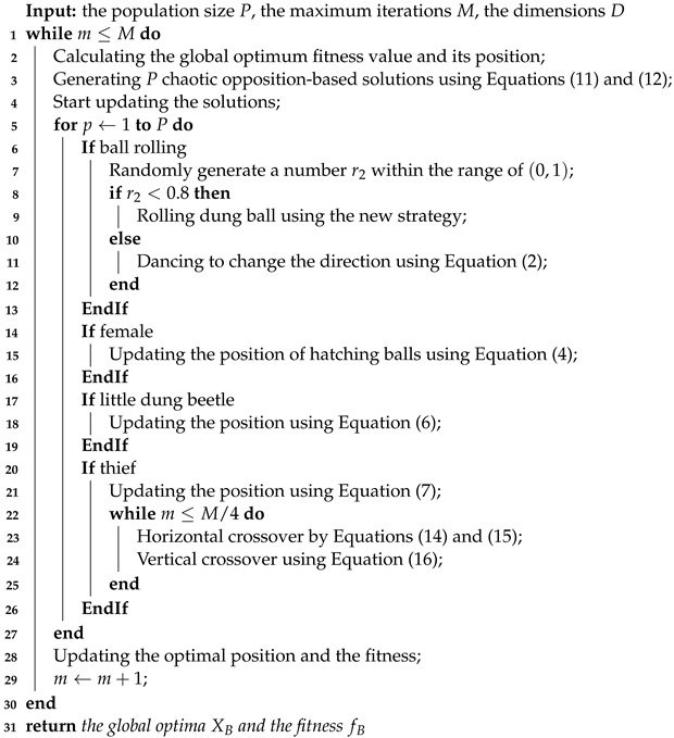
