Enhancing Portfolio Performance through Financial Time-Series Decomposition-Based Variational Encoder-Decoder Data Augmentation

Abstract

The objective of portfolio diversification is to reduce risk and potentially enhance returns by spreading investments across different asset classes. Existing portfolio diversification models have traditionally been trained on historical financial time series data. However, several issues arise with historical financial time series data, making it challenging to train models effectively to achieve the portfolio diversification objective: an insufficient amount of training data and the uncertainty deficiency problem, wherein the uncertainty that existed in the past is not visible in the present. Insufficient datasets, characterized by small data size, result in information asymmetry and compromise portfolio performance. This limitation underscores the importance of adopting a pattern-centric data augmentation approach, capable of unveiling hidden patterns and structures within the financial time series data. To address these challenges, this paper introduces the financial time series decomposition-based variational encoder-decoder (FED) method to augment financial time series data, overcoming the limitations of insufficient training data and providing a more realistic and dynamic simulation of the financial market environment. By decomposing the data into distinct components, such as trend, dispersion, and residual, FED leverages pattern-centric data augmentation within the financial time series data. In the environment generated using the FED method, this paper proposes a two-class portfolio diversification, called FED2Port. It integrates stochastic elements into the reward function, enabling a reinforcement learning algorithm to learn from a comprehensive spectrum of financial market uncertainties. The experimental results demonstrate that the proposed model significantly enhances portfolio performance.

1. Introduction

Financial investments involve a trade-off between risk and return. Higher potential returns usually come with higher risks. A diversified portfolio is an investment strategy that involves spreading investments across different asset classes. Large-scale funds, such as national pensions worldwide, invest in a diverse range of assets. In most countries, equities and bills and bonds were the two main asset classes in which pension capital was invested in 2020, accounting for more than half of the investment in 35 out of 38 OECD countries and four reporting non-OECD G20 jurisdictions [1]. The Melbourne Mercer Global Pension Index (MMGPI) considers a split between growth and defensive assets [2]. Growth assets typically include high-risk assets, such as equities, property, and some alternative assets. On the other hand, defensive assets include low-risk assets, such as bills and bonds, as well as cash and deposits.

The present study classifies financial assets into two broad categories based on their inherent characteristics and the level of associated risk: high-risk and low-risk assets. This classification is similar to the MMGPI categorization, with growth representing high-risk and defensive representing low-risk. Such categorization assists investors in making well-informed portfolio decisions, balancing risk tolerance and investment goals. Investments in high-risk assets can offer significantly large returns, making them attractive to investors seeking aggressive growth, but they also come with a higher likelihood of losses. On the other hand, investments in low-risk assets are often considered safer for preserving capital and generating modest, consistent returns. Two-class portfolio diversification involves spreading investments between these two classes of assets to reduce the overall portfolio risk.

A buy-and-hold strategy is a long-term investment approach where an investor buys assets and holds onto them for an extended period, regardless of short-term market fluctuations. Portfolio rebalancing is the process of periodically adjusting the weights of assets in a portfolio. The tangency portfolio among Markowitz optimization [3], risk budgeting [4,5], recurrent reinforcement learning (RRL) [6,7], and deep deterministic policy gradient (DDPG) [8,9] aims to find the optimal proportion of assets within a given period. Traditional portfolio diversification models [3,4,5] aim to optimize the allocation of assets in a portfolio to balance risk and return. Markowitz optimization [3] provides a mathematical approach for constructing an investment portfolio that maximizes the expected return for a given level of risk or minimizes the risk for an expected return. Risk budgeting [4,5] involves allocating risk across different assets or asset classes based on predefined risk constraints. This strategy aims to control and manage the portfolio risk effectively. Reinforcement learning (RL) portfolio diversification models [6,7,8,9,10,11] make decisions by interacting with an environment to maximize a cumulative reward signal. While RRL [6,7,10] aims to learn the optimal policy by maximizing the reward functions, DDPG [8,9] achieves this goal by adjusting the parameters of the actor and critic networks iteratively using optimization techniques.

Existing portfolio diversification models have a common deficit; they are trained using only historical financial time series data. On the other hand, historical financial time series data have the following problems.

• Uncertainty deficiency. Both the financial market and its empirical time series data contain inherent uncertainty. At some point, probabilities were assigned to different events or market scenarios, including rises, falls, and magnitudes of changes, with non-zero probabilities. On the other hand, as time elapses, all past events collapse into a single outcome. Consequently, only one event is assigned a 100% probability, and the probabilities of all other events are set to 0%. This phenomenon, termed uncertainty deficiency, suggests that historical financial time series data only represent a sequence of singular events, lacking the diversity of market uncertainties that existed in the past. Ignoring financial market uncertainty can lead to overly confident models that fail to account for unforeseen risks. RL algorithms or traditional models optimized solely based on historical financial time series data may lack robustness and show poor capability when applied to novel or extreme events.
• Insufficient amount of training data. Historical financial time-series datasets are often not large enough for training due to financial market uncertainty. For example, even with 10 years of daily data for an asset class (250 trading days in a year × 10 years = 2500), the amount is relatively small, only 2.5k. Insufficient datasets, characterized by small data size, result in information asymmetry and compromise portfolio performance.

Good results are not possible in the face of future uncertainty because of these problems. A financial time series decomposition-based variational encoder-decoder (FED) data augmentation is proposed to address the challenges of financial market uncertainty and insufficient training data, providing a more realistic and dynamic simulation of the financial market environment. Under the environment generated by FED, this paper proposes a two-class portfolio diversification (FED2Port), allowing the RL algorithm to learn from a comprehensive spectrum of financial market uncertainties.

The main contributions of this paper are as follows.

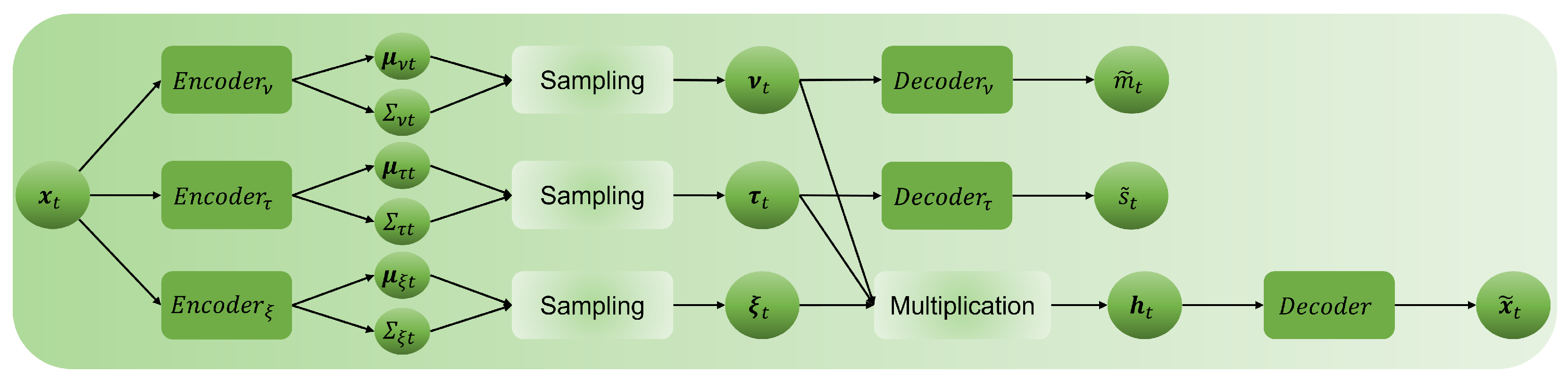
• FED for Financial Time Series Data Augmentation. The first contribution introduces an innovative financial time series data augmentation called the FED. Generating nonstationary financial time series data is deemed challenging, and FED addresses this challenge by leveraging decomposition techniques, separating the financial time series into distinct components (trend, dispersion, and residual). Based on the encoder-decoder architecture, the FED method utilizes latent variables further decomposed into components. This pattern-centric approach provides a profound understanding of the underlying structure of financial time series data, unveiling the hidden patterns or structures and offering insights into factors influencing observed trends and fluctuations. FED captures the distributions of latent variable components, generating more realistic financial time series data. In doing so, the FED method revives some of the past uncertainty that had disappeared, compensating for the problems of uncertainty deficiency and an insufficient amount of training data.
• FED2Port for Decision-Making under Financial Market Uncertainty. The second contribution is the proposal of FED2Port as a novel diversification approach to enhance the efficiency of RL algorithms. Specifically tailored for RL portfolio diversification models, FED2Port addresses the uncertainty deficiency problem inherent in historical financial time series data. FED2Port trains the RL algorithm under the financial market environment generated using the FED. This environment simulation incorporates stochastic elements in the reward function, enabling the algorithm to learn from a more comprehensive spectrum of financial market uncertainties. Therefore, FED2Port improves the adaptability of the algorithm significantly, empowering it to make well-informed decisions in the face of future uncertainty, ultimately enhancing portfolio performance.

2. Related Work

Financial time series data generation plays a significant role in RL portfolio diversification models by addressing the challenges of financial market uncertainty and enhancing portfolio performance. Simulating the financial market environment with additional scenarios and variations can help improve the robustness of portfolio diversification. This ensures that the RL algorithm is exposed to a broader range of market conditions. The two most prominent types of generative models are the generative adversarial nets (GANs) [12,13] and variational autoencoders (VAEs) [14,15].

GANs usually generate more realistic data but face training stability and sampling diversity challenges. GANs are based on a two-player minimax game with value function $V(G,D)$:

$$\begin{array}{cc}\hfill \underset{G}{min}\underset{D}{max}V(G,D):=& {\mathbb{E}}_{x\sim p_{data}\left(x\right)}[logD\left(x\right)]\hfill \\ \hfill & +{\mathbb{E}}_{z\sim p_Z\left(z\right)}[log(1-D\left(G\left(z\right)\right))]\hfill \end{array}$$

where $z,G$, and D are random noise, a generator, and a discriminator, respectively. GANs involve training a generator and a discriminator in a competitive setting, which can sometimes lead to training instabilities, mode collapse, or difficulties in convergence. Time-series GAN (TimeGAN) [16] and real-world time series GAN (RTSGAN) [17] are designed to generate synthetic data that closely resemble real-world time series data. In TimeGAN, the generator produces embeddings, and the recovery produces time series data based on the generated embeddings. RTSGAN shares similarities with TimeGAN but sets itself apart by specializing in generating time series data with variable lengths. They do not address the nonstationary financial time series data generation.

VAEs often exhibit more stable training dynamics compared to GANs. VAEs explicitly model the generative process by assuming a specific form for the latent variable distribution. This can be advantageous in scenarios where understanding the generative process is crucial. VAEs aim to maximize the probability of the generated output with respect to the input and produce an output from a target distribution by compressing the input into a latent space. VAEs can learn via maximum likelihood using a variational approach to maximize the evidence lower bound (ELBO) as follows:

$$\mathit{ELBO}=-D_{KL}[q_{\varphi }\left(z\right|x)\left|\right|p\left(z\right)]+{\mathbb{E}}_{q_{\varphi }\left(z\right|x)}[log{p}_{\theta }\left(x\right|z)]$$

where $q_{\varphi }\left(z\right|x)$ is an approximate posterior distribution for the latent variables, also known as a probabilistic encoder; $p\left(z\right)$ is a prior over the latent variables; $p_{\theta }\left(x\right|z)$ is a likelihood function, also known as a probabilistic decoder.

Time series decomposition [18,19,20,21,22,23,24,25,26] aims to decompose a time series into its components structurally and interpretably. These components typically include the trend, seasonal, and residual components. The trend component represents the long-term direction or underlying movement in the financial time series data, capturing the overall trajectory, which can be either linear or nonlinear. It helps identify whether the financial time series data generally increases or decreases over time. The seasonal component captures the periodic patterns and fluctuations within a year or specified period, elucidating regular, predictable movements in the financial time series data. The cyclical component represents longer-term fluctuations tied to economic or business cycles, spanning multiple years and identifying broader economic trends. The residual component, the error term or reminder, accounts for random and unexplained variability in the financial time series data, not attributable to the trend, seasonal, or cyclical components. Time series decomposition can be expressed in additive or multiplicative forms. An additive decomposition [22] would be written as

$$y_t=T_t+S_t+R_t$$

A multiplicative decomposition [22] would be written as

$$y_t=T_t\times S_t\times R_t$$

where $y_t,S_t,T_t$, and $R_t$ are the data, seasonal component, trend component, and residual component, respectively, all at time t. The additive decomposition is appropriate when the magnitude of the seasonal fluctuations or the variation around the trend does not change as the level of the time series increases. The multiplicative decomposition is more appropriate when the variation in the seasonal pattern or the variation around the trend is proportional to the time series level [22].

STD decomposition [26] extracts the components of the seasonality, trend, and dispersion, it is expressed as

$$y_t=S_t\times D_t+T_t$$

where $y_t,S_t,D_t$, and $T_t$ are the data, seasonal component, dispersion component, and trend component, respectively, all at time t. STD with a reminder component [26], called STDR, is defined as follows:

$$y_t=S_t^{\prime }\times D_t+T_t+R_t$$

where $S_t^{\prime }$ is an averaged seasonal component, and $R_t$ is a reminder component, all at time t.

Decomposition is a crucial tool in analyzing and simulating nonstationary financial time series data, providing insights into changing patterns and helping simulators better understand and model the complexities of financial markets.

The Markowitz optimization [3], known as modern portfolio theory (MPT), provides a mathematical approach to constructing portfolios to maximize the expected returns while minimizing risk. The tangency portfolio represents the optimal portfolio that maximizes a risk-adjusted return measure, the Sharpe ratio [27]. Risk budgeting [4,5] is a portfolio construction approach that involves allocating risk among different assets based on predefined risk constraints. A risk budgeting model helps to manage and control the overall risk of a portfolio while optimizing returns. Previous studies [3,4,5] relied on the assumption of a stationary market. The Black–Litterman model [28] is an asset allocation framework that combines market equilibrium assumptions [29] with an investor’s subjective views. Applying the Black–Litterman model requires the availability of expert views or a predictive model that can represent those expert views.

Maximizing future rewards typically involves optimizing a sequence of decisions or actions to achieve the best possible outcomes. It is a fundamental problem in various fields, including reinforcement learning. Ref. [6] introduced an RL model called recurrent reinforcement learning (RRL) for portfolio management. They used the Sharpe ratio as the reward. A previous study [7] used the modified RRL, which optimizes the Sharpe ratio with batch learning. The deep deterministic policy gradient (DDPG) [30] was used for portfolio management [8,9]. RL portfolio diversification models [6,7,8,9] can construct optimal portfolios that achieve the best possible rewards, such as the expected return, the Sharpe ratio [27], the Sortino ratio [31], or the market-adaptive ratio [32]. The Sharpe ratio [27] relates the excess returns on a portfolio to its risk, the standard deviation of the excess return. The market-adaptive ratio [32] is a risk-adjusted return based on a market-type measure, rho. This ratio is a general form of the Sharpe ratio, considering the characteristics of the market types. During bull markets, the focus is on seeking high returns and embracing risk. In contrast, it aims to preserve capital and minimize risk during bear markets. The Sortino ratio [31] focuses on the downside risk. RL portfolio diversification models leverage insights gained from data analysis instead of relying on an assumption. On the other hand, they use observed historical environments to estimate the model parameters that lead to the uncertainty deficiency and the shortage of training data problems.

3. Proposed Methods

The d-day log-return vector of the high-risk asset (or the low-risk asset) at time t is defined as

$$\begin{array}{c}\hfill {\mathit{x}}_t=\left[\begin{array}{c}{x}_{t-d+1}\\ x_{t-d+2}\\ \cdots \\ x_t\end{array}\right]=\left[\begin{array}{c}log\frac{p_{t-d+1}}{p_{t-d}}\\ log\frac{p_{t-d+2}}{p_{t-d+1}}\\ \cdots \\ log\frac{p_t}{p_{t-1}}\end{array}\right]\end{array}$$

(1)

where $p_t$ is the price of a high-risk asset (or the low-risk asset) at time t.

3.1. FED

The encoder-decoder architecture encourages the latent space to have meaningful representations of the data, which is advantageous for operations like interpolation or feature manipulation. Based on this architecture, the FED method utilizes latent variables further decomposed into components. This approach provides a profound understanding of the underlying structure of financial time series data, unveiling the hidden patterns or structures and offering insights into factors influencing observed trends and fluctuations.

Time series decomposition is a fundamental technique in time series analysis that separates complex time series data into individual components, helping understand the underlying dynamics. Most time series decomposition methods have focused on the trend, seasonal, and residual components. Previous work [26] considers a component related to the dispersion of the time series. The trend and dispersion components are crucial for generating financial time series data due to their nonstationary property. FED incorporates components of the trend, dispersion, and residual. The trend component, $m_t$, is the mean return at time t, representing the direction of financial time series data. The dispersion component, $s_t$, is the standard deviation of the return at time t, representing the fluctuation of financial time series data. The residual component accounts for the unexplained variability in the financial time series data. The primary concept of the proposed model is to apply decomposition into the hidden space. By emphasizing these components, FED leverages pattern-centric data augmentation within the financial time series data.

Assume that data ${\tilde{\mathit{x}}}_t$ are generated by a decoder with a probabilistic latent variable, ${\mathit{h}}_t$.

$${\tilde{\mathit{x}}}_t=D\left({\mathit{h}}_t\right)$$

(2)

The FED method is based on the latent variable decomposition,

$${\mathit{h}}_t={\mathit{\nu }}_t\times {\mathit{\tau }}_t\times {\mathit{\xi }}_t$$

(3)

where ${\mathit{\nu }}_t\sim N({\mathit{\mu }}_{\nu t},{\mathrm{\Sigma }}_{\nu t})$ is a probabilistic trend component of the latent variable, ${\mathbf{\tau }}_t\sim N({\mathit{\mu }}_{\mathit{\tau }t},{\mathrm{\Sigma }}_{\mathit{\tau }t})$ is a probabilistic dispersion component of the latent variable, and ${\mathbf{\xi }}_t\sim N({\mathit{\mu }}_{\xi t},{\mathrm{\Sigma }}_{\xi t})$ is a probabilistic residual component of the latent variable, all at time t.

The product of two multivariate normal distributions results in another multivariate normal distribution [33], which is valuable and highly useful in the proposed model. Consequently, the parameters of the probabilistic hidden variable, ${\mathit{h}}_t\sim N({\mathit{\mu }}_{ht},{\mathrm{\Sigma }}_{ht})$ were calculated, as follows:

$$\begin{array}{cc}\hfill N({\mathit{\mu }}_{\nu t},{\mathrm{\Sigma }}_{\nu t})\times N({\mathit{\mu }}_{\mathit{\tau }t},{\mathrm{\Sigma }}_{\mathit{\tau }t})\times N({\mathit{\mu }}_{\xi t},{\mathrm{\Sigma }}_{\xi t})& =N({\mathit{\mu }}_{1t},{\mathrm{\Sigma }}_{1t})\times N({\mathit{\mu }}_{\xi t},{\mathrm{\Sigma }}_{\xi t})\hfill \\ \hfill & =N({\mathit{\mu }}_{ht},{\mathrm{\Sigma }}_{ht})\hfill \end{array}$$

(4)

where

$$\begin{array}{cc}\hfill {\mathrm{\Sigma }}_{1t}& ={({\mathrm{\Sigma }}_{\nu t}^{-1}+{\mathrm{\Sigma }}_{\mathit{\tau }t}^{-1})}^{-1}\hfill \\ \hfill {\mathit{\mu }}_{1t}& ={\mathrm{\Sigma }}_{1t}{\mathrm{\Sigma }}_{\nu t}^{-1}{\mathit{\mu }}_{\nu t}+{\mathrm{\Sigma }}_{1t}{\mathrm{\Sigma }}_{\tau t}^{-1}{\mathit{\mu }}_{\tau t}\hfill \end{array}$$

(5)

and

$$\begin{array}{cc}\hfill {\mathrm{\Sigma }}_{ht}& ={({\mathrm{\Sigma }}_{1t}^{-1}+{\mathrm{\Sigma }}_{\xi t}^{-1})}^{-1}\hfill \\ \hfill & ={({\mathrm{\Sigma }}_{\nu t}^{-1}+{\mathrm{\Sigma }}_{\mathit{\tau }t}^{-1}+{\mathrm{\Sigma }}_{\xi t}^{-1})}^{-1}\hfill \\ \hfill {\mathit{\mu }}_{ht}& ={\mathrm{\Sigma }}_{ht}{\mathrm{\Sigma }}_{1t}^{-1}{\mathit{\mu }}_{1t}+{\mathrm{\Sigma }}_{ht}{\mathrm{\Sigma }}_{\xi t}^{-1}{\mathit{\mu }}_{\xi t}\hfill \\ \hfill & ={\mathrm{\Sigma }}_{ht}{\mathrm{\Sigma }}_{\nu t}^{-1}{\mathit{\mu }}_{\nu t}+{\mathrm{\Sigma }}_{ht}{\mathrm{\Sigma }}_{\mathit{\tau }t}^{-1}{\mathit{\mu }}_{\mathit{\tau }t}+{\mathrm{\Sigma }}_{ht}{\mathrm{\Sigma }}_{\xi t}^{-1}{\mathit{\mu }}_{\xi t}\hfill \end{array}$$

(6)

FED employs three encoders to model the three probabilistic components of the latent variables, including trend (return), dispersion (standard deviation), and residual. Similar to reference [14], the reparameterization trick was used. Figure 1 illustrates the general framework of FED.

Figure 1. General framework of financial time series decomposition-based variational encoder-decoder (FED). ${\mathit{x}}_t$ is the d-day log-return vector of the high-risk asset (or the low-risk asset) at time t. ${\tilde{m}}_t$, ${\tilde{s}}_t$, and ${\tilde{\mathit{x}}}_t$ are the generated trend (return), the generated dispersion (standard deviation), and the generated d-day log-return vector of the high-risk asset (or the low-risk asset), respectively, all at time t. ${\mathit{\nu }}_t\sim N({\mathit{\mu }}_{\nu t},{\mathrm{\Sigma }}_{\nu t})$ is a probabilistic trend component of the latent variable, ${\mathbf{\tau }}_t\sim N({\mathit{\mu }}_{\tau t},{\mathrm{\Sigma }}_{\tau t})$ is a probabilistic dispersion component of the latent variable, and ${\mathit{\xi }}_t\sim N({\mathit{\mu }}_{\xi t},{\mathrm{\Sigma }}_{\xi t})$ is a probabilistic residual component of the latent variable. ${\mathit{h}}_t={\mathit{\nu }}_t\times {\mathbf{\tau }}_t\times {\mathit{\xi }}_t$ is the decomposed latent variable.

The marginal log-likelihood of the trend $m_t$:

$$\begin{array}{cc}\hfill logp\left(m_t\right)& =log\int p_{{\theta }_{\nu }}\left(m_t\right|{\mathit{\nu }}_t)p\left({\mathit{\nu }}_t\right)d{\mathit{\nu }}_t\hfill \\ \hfill & =log\int \frac{q_{{\varphi }_{\nu }}\left({\nu }_t\right|{\mathit{x}}_t)}{q_{{\varphi }_{\nu }}\left({\mathit{\nu }}_t\right|{\mathit{x}}_t)}{p}_{{\theta }_{\nu }}\left(m_t\right|{\mathit{\nu }}_t)p\left({\mathit{\nu }}_t\right)d{\mathit{\nu }}_t\hfill \\ \hfill & \ge \int q_{{\varphi }_{\nu }}\left({\mathit{\nu }}_t\right|{\mathit{x}}_t)log\left[\frac{p\left({\mathit{\nu }}_t\right)}{q_{{\varphi }_{\nu }}\left({\mathit{\nu }}_t\right|{\mathit{x}}_t)}{p}_{{\theta }_{\nu }}\left(m_t\right|{\mathit{\nu }}_t)\right]d{\mathit{\nu }}_t\hfill \\ \hfill & =-\int q_{{\varphi }_{\nu }}\left({\mathit{\nu }}_t\right|{\mathit{x}}_t)log\left[\frac{q_{{\varphi }_{\nu }}\left({\mathit{\nu }}_t\right|{\mathit{x}}_t)}{p\left({\mathit{\nu }}_t\right)}\right]d{\mathit{\nu }}_t+\int q_{{\varphi }_{\nu }}\left({\mathit{\nu }}_t\right|{\mathit{x}}_t)log\left[p_{{\theta }_{\nu }}\left(m_t\right|{\mathit{\nu }}_t)\right]d{\mathit{\nu }}_t\hfill \\ \hfill & =-D_{KL}\left[q_{{\varphi }_{\nu }}\left({\mathit{\nu }}_t\right|{\mathit{x}}_t)\left|\right|p\left({\mathit{\nu }}_t\right)\right]+{\mathbb{E}}_{q_{{\varphi }_{\nu }}\left({\mathit{\nu }}_t\right|{\mathit{x}}_t)}\left[log{p}_{{\theta }_{\nu }}\left(m_t\right|{\mathit{\nu }}_t)\right]\hfill \end{array}$$

(7)

where $p_{{\theta }_{\mathit{\nu }}}\left(m_t\right|{\mathit{\nu }}_t)$ is the conditional probability distribution of the trend $m_t$ given the latent variable ${\mathit{\nu }}_t$, modeled by a decoder and the sampling of the latent variable, and $q_{{\varphi }_{\nu }}\left({\mathit{\nu }}_t\right|{\mathit{x}}_t)$ is the conditional probability distribution of the latent variable ${\mathit{\nu }}_t$ given data ${\mathit{x}}_t$, modeled by an encoder and the reparameterization trick. The above bound is the evidence lower bound (ELBO).

Similarly, the marginal log-likelihood of dispersion $s_t$ is expressed as

$$\begin{array}{cc}\hfill logp\left(s_t\right)& =log\int p_{{\theta }_{\tau }}\left(s_t\right|{\mathit{\tau }}_t)p\left({\mathit{\tau }}_t\right)d{\mathit{\tau }}_t\hfill \\ \hfill & =log\int \frac{q_{{\varphi }_{\tau }}\left({\mathit{\tau }}_t\right|{\mathit{x}}_t)}{q_{{\varphi }_{\tau }}\left({\mathit{\tau }}_t\right|{\mathit{x}}_t)}{p}_{{\theta }_{\tau }}\left(s_t\right|{\mathit{\tau }}_t)p\left({\mathit{\tau }}_t\right)d{\mathit{\tau }}_t\hfill \\ \hfill & \ge -D_{KL}\left[q_{{\varphi }_{\tau }}\left({\mathit{\tau }}_t\right|{\mathit{x}}_t)\left|\right|p\left({\mathit{\tau }}_t\right)\right]+{\mathbb{E}}_{q_{{\varphi }_{\tau }}\left({\mathit{\tau }}_t\right|{\mathit{x}}_t)}\left[log{p}_{{\theta }_{\tau }}\left(s_t\right|{\mathit{\tau }}_t)\right]\hfill \end{array}$$

(8)

where $p_{{\theta }_{\mathit{\tau }}}\left(s_t\right|{\mathit{\tau }}_t)$ is the conditional probability distribution of the dispersion $s_t$ given the latent variable ${\mathit{\tau }}_t$, modeled by a decoder and the sampling of the latent variable, and $q_{{\varphi }_{\tau }}\left({\mathit{\tau }}_t\right|{\mathit{x}}_t)$ is the conditional probability distribution of the latent variable ${\mathit{\tau }}_t$ given data ${\mathit{x}}_t$, modeled by an encoder and the reparameterization trick.

Similarly, the marginal log-likelihood of data ${\mathit{x}}_t$ is expressed as

$$\begin{array}{cc}\hfill logp\left({\mathit{x}}_t\right)& =log\int p_{\theta }\left({\mathit{x}}_t\right|{\mathit{h}}_t)p\left({\mathit{h}}_t\right)d{\mathit{h}}_t\hfill \\ \hfill & =log\int \frac{q_{\varphi }\left({\mathit{h}}_t\right|{\mathit{x}}_t)}{q_{\varphi }\left({\mathit{h}}_t\right|{\mathit{x}}_t)}{p}_{\theta }\left({\mathit{x}}_t\right|{\mathit{h}}_t)p\left({\mathit{h}}_t\right)d{\mathit{h}}_t\hfill \\ \hfill & \ge -D_{KL}\left[q_{\varphi }\left({\mathit{h}}_t\right|{\mathit{x}}_t)\left|\right|p\left({\mathit{h}}_t\right)\right]+{\mathbb{E}}_{q_{\varphi }\left({\mathit{h}}_t\right|{\mathit{x}}_t)}\left[log{p}_{\theta }\left({\mathit{x}}_t\right|{\mathit{h}}_t)\right]\hfill \end{array}$$

(9)

where $p_{\theta }\left({\mathit{x}}_t\right|{\mathit{h}}_t)$ is the conditional probability distribution of data ${\mathit{x}}_t$ given the latent variable ${\mathit{h}}_t$, modeled by a decoder and the sampling of the latent variable, and $q_{\varphi }\left({\mathit{h}}_t\right|{\mathit{x}}_t)$ is the conditional probability distribution of the latent variable ${\mathit{h}}_t$ given data ${\mathit{x}}_t$, modeled by encoders and the reparameterization trick. The FED method aims to maximize the combination of the above three bounds as follows:

$$\begin{array}{cc}\hfill L_{FED}& :=\alpha \left(-D_{KL}\left[q_{{\varphi }_{\nu }}\left({\mathit{\nu }}_t\right|{\mathit{x}}_t)\left|\right|p\left({\mathit{\nu }}_t\right)\right]+{\mathbb{E}}_{q_{{\varphi }_{\nu }}\left({\mathit{\nu }}_t\right|{\mathit{x}}_t)}\left[log{p}_{{\theta }_{\nu }}\left(m_t\right|{\mathit{\nu }}_t)\right]\right)\hfill \\ \hfill & +\beta \left(-D_{KL}\left[q_{{\varphi }_{\tau }}\left({\mathit{\tau }}_t\right|{\mathit{x}}_t)\left|\right|p\left({\mathit{\tau }}_t\right)\right]+{\mathbb{E}}_{q_{{\varphi }_{\tau }}\left({\mathit{\tau }}_t\right|{\mathit{x}}_t)}\left[log{p}_{{\theta }_{\tau }}\left(s_t\right|{\mathit{\tau }}_t)\right]\right)\hfill \\ \hfill & +\gamma \left(-D_{KL}\left[q_{\varphi }\left({\mathit{h}}_t\right|{\mathit{x}}_t)\left|\right|p\left({\mathit{h}}_t\right)\right]+{\mathbb{E}}_{q_{\varphi }\left({\mathit{h}}_t\right|{\mathit{x}}_t)}\left[log{p}_{\theta }\left({\mathit{x}}_t\right|{\mathit{h}}_t)\right]\right)\hfill \end{array}$$

(10)

where $\alpha$, $\beta$, and $\gamma$ are hyperparameters that control the importance of each task.

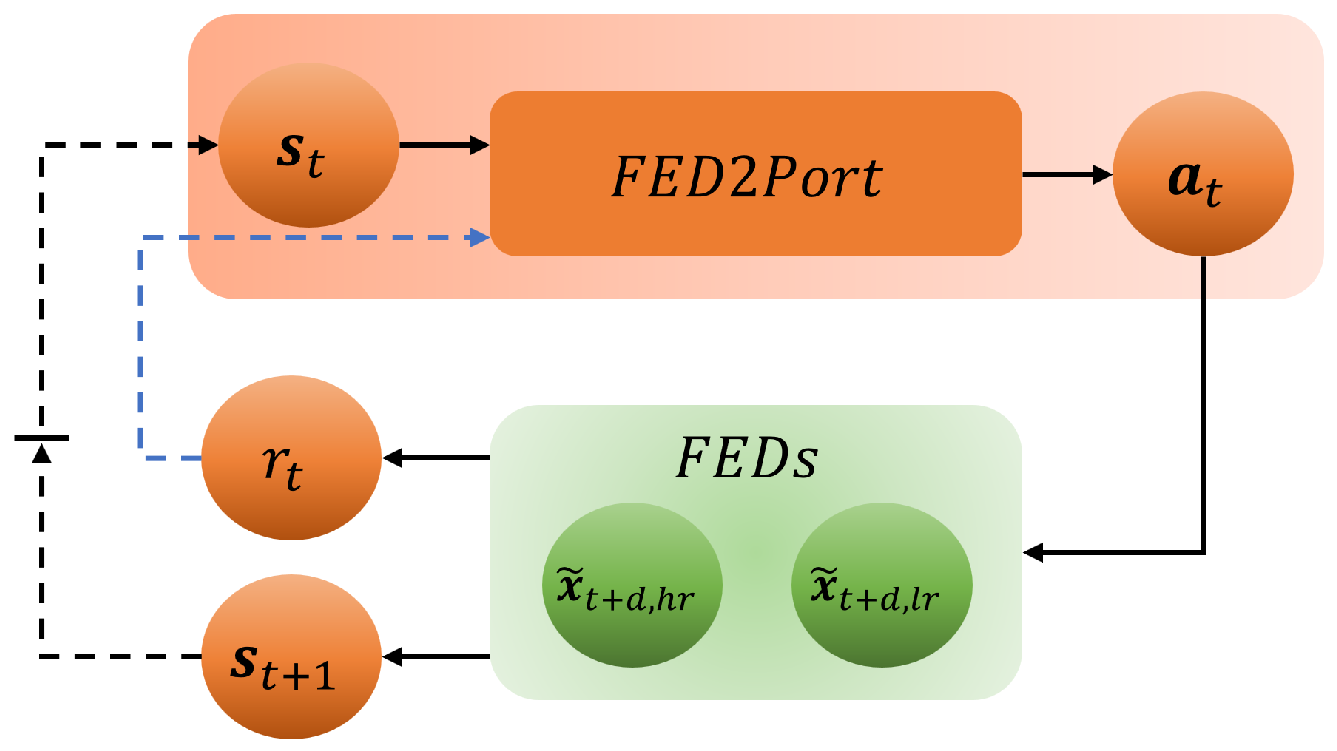
3.2. FED2Port

The environment of the FED2Port is defined as follows.

• The action is defined as the weight vector:

  $$\begin{array}{c}\hfill {\mathit{a}}_t=\left[\begin{array}{c}{a}_{t,hr}\\ a_{t,lr}\end{array}\right]\end{array}$$

  (11)

  where $a_{t,hr}$ and $a_{t,lr}\ge 0$ represent the weights of a high-risk asset and a low-risk asset, respectively, with the constraint that $a_{t,hr}+a_{t,lr}=1$.
• The state is defined as the portfolio return ${\mathit{s}}_t$:

  $${\mathit{s}}_t=a_{t-1,hr}{\mathit{x}}_{t,hr}+a_{t-1,lr}{\mathit{x}}_{t,lr}$$

  (12)

  where ${\mathit{x}}_{t,hr}$ and ${\mathit{x}}_{t,lr}$ are the d-day log-return vectors of the high-risk and low-risk assets, respectively.
• The reward is defined as the market-adaptive ratio [32]:

  $$r_t({\tilde{\mathit{x}}}_{t+d,hr},{\tilde{\mathit{x}}}_{t+d,lr},{\mathit{a}}_t)=\frac{{({\overline{R}}_p-R_f)}^{{\rho }_{hr}}}{{\sigma }_p^{1/{\rho }_{hr}}}$$

  (13)

  where ${\rho }_{hr}=\frac{2}{1+e^{-R_{hr}}}$ represents the rho of the high-risk asset; $R_{hr}$ is the return of the high-risk asset, ${\tilde{\mathit{x}}}_{t+d,hr}$ and ${\tilde{\mathit{x}}}_{t+d,lr}$ are the generated log-return vectors of the high-risk and low-risk assets, respectively. FED methods are used for high-risk and low-risk assets. ${\overline{R}}_p$ and ${\sigma }_p$ represent the expected return and standard deviation of the total portfolio, respectively, and $R_f$ is the risk-free rate. In this paper, the risk-free rate equals zero. By using the market-adaptive ratio as the reward, FED2Port can take into account market characteristics such as bull and bear markets.

The agent, ${\pi }_{\omega }$, receives the portfolio return and selects an action.

$${\mathit{a}}_t={\pi }_{\omega }\left({\mathit{s}}_t\right)$$

(14)

It controls the policy using an evaluation of the reward. Figure 2 illustrates the general framework of FED2Port.

Figure 2. General framework of two-class portfolio diversification (FED2Port). ${\mathit{s}}_t$ and ${\mathit{a}}_t$ are the state and the action, respectively, at time t. ${\tilde{\mathit{x}}}_{t+d,hr}$ and ${\tilde{\mathit{x}}}_{t+d,lr}$ represent the generated log-return vectors of the high-risk and low-risk assets, respectively, at time t. $r_t$ is the reward at time t.

The objective of FED2Port is to maximize the expected reward,

$$\underset{\omega }{max}{\mathbb{E}}_{{\tilde{\mathit{x}}}_{t+d,hr},{\tilde{\mathit{x}}}_{t+d,lr}}\left[r_t({\tilde{\mathit{x}}}_{t+d,hr},{\tilde{\mathit{x}}}_{t+d,lr},{\mathit{a}}_t)\right]$$

(15)

4. Experiment

4.1. Dataset

FED2Port aims to allocate the total investment into two classes: high-risk and low-risk assets. This paper considers three stock indices and three bond funds (Table 1) in the experiment. The daily data from January 2010 to December 2022 (https://finance.yahoo.com/ accessed on 1 October 2023) were included. To initialize models, they were trained using the five-year data from January 2010 to December 2014 for each dataset. Then, we tested the model using eight-year data, from January 2015 to December 2022.

Table 1. Assets.

Class	Symbol	Explanation
High-risk assets	SP500	S&P500 Index
	DAX	DAX Index
	KOSPI	KOSPI Index
Low-risk assets	BND	Vanguard Total Bond Market Index Fund
	BSV	Vanguard Short-Term Bond Index Fund
	VCIT	Vanguard Intermediate-Term Treasury Index Fund

Figure 3 depicts the price data of the assets, while Table 2 lists the differences between stock market indices and bond funds. While stock market indices carry higher risk, bond funds offer lower risk. Nine two-class portfolios (Table 3) were considered, comprising three stock indices and three bond funds (Table 1), to assess the performance of the proposed model.

Figure 3. Graphs of the price data of the assets.

Table 2. Statistic of funds during test period.

	SP500	DAX	KOSPI	BND	BSV	VCIT
The standard deviation of the portfolio return	0.5221	0.6125	0.5564	0.1429	0.0590	0.1702

Table 3. Portfolios.

	Portfolio	Low-Risk Asset	High-Risk Asset
1	BND&SP500	Vanguard Total Bond Market Index Fund	S&P500 Index
2	BND&DAX	Vanguard Total Bond Market Index Fund	DAX Index
3	BND&KOSPI	Vanguard Total Bond Market Index Fund	KOSPI Index
4	BSV&SP500	Vanguard Short-Term Bond Index Fund	S&P500 Index
5	BSV&DAX	Vanguard Short-Term Bond Index Fund	DAX Index
6	BSV&KOSPI	Vanguard Short-Term Bond Index Fund	KOSPI Index
7	VCIT&SP500	Vanguard Intermediate-Term Treasury Index Fund	S&P500 Index
8	VCIT&DAX	Vanguard Intermediate-Term Treasury Index Fund	DAX Index
9	VCIT&KOSPI	Vanguard Intermediate-Term Treasury Index Fund	KOSPI Index

4.2. Benchmarks

For comparison, several benchmarks (Table 4) were considered, including buy-and-hold strategies, traditional portfolio diversification models, and RL portfolio diversification models. The buy-and-hold strategy is a long-term investment approach in portfolio management where an investor buys financial assets and holds onto them for an extended period, regardless of short-term market fluctuations. Traditional portfolio diversification models help construct portfolios that align with the investors’ risk tolerance and return objectives. RL portfolio diversification models showcase the adaptability and learning capabilities of reinforcement learning.

Table 4. Comparison benchmarks.

	Model	Explanation
1	100% low-risk asset portfolio	Buy-and-Hold strategies
2	Equally Weighted
3	100% high-risk asset portfolio
4	Tangency portfolio	Traditional portfolio diversification models
5	Risk Budgeting
6	RRL	Historical data-based RL portfolio diversification models
7	DDPG
8	TimeGAN2Port	Data augmentation-based RL portfolio diversification models
9	RTSGAN2Port

4.3. Performance Measures

The expected portfolio return, the standard deviation of the portfolio return, and the Sharpe ratio were considered to evaluate the effectiveness of portfolio strategies.

The expected portfolio return (Profit) is expressed as

$${\mu }_p=t\times {\overline{R}}_p$$

(16)

where t is the length of the test period, and ${\overline{R}}_p$ is the daily mean return of the portfolio. The expected portfolio return provides insight into the overall portfolio performance, capturing the total change in value over time.

The standard deviation of the portfolio return (Risk) is expressed as follows:

$${\sigma }_p=\sqrt{t\times \frac{{\sum }_{i=1}^t{(R_{p,i}-{\overline{R}}_p)}^2}{t-1}}$$

(17)

where $R_{p,i}$ is a daily return of the portfolio at time i. The standard deviation of the portfolio return is a key metric in assessing the risk associated with a portfolio. A higher standard deviation indicates greater variability in returns, suggesting higher risk, while a lower standard deviation implies more stability.

The Sharpe ratio is a risk-adjusted return that evaluates the portfolio performance, which was calculated using expected return and risk during the test period, as follows.

$$\mathit{Sharpe\; ratio}=\frac{{\mu }_p}{{\sigma }_p}$$

(18)

4.4. Experimental Results

Network architectures in Figure 4 were used for the encoder and decoder of the FED method. The dimensions of the latent variables were set to 100. The network architecture in Figure 5 was used for the FED2Port agent, ${\pi }_{\omega }$, which utilizes the Softmax function to generate portfolio weights. A rolling window approach was implemented to retrain the FED2Port model annually from January 2015 to December 2022. The total portfolios were rebalanced for each month (20 trading days). The Profit (Equation (16)), Risk (Equation (17)), and Sharpe ratio (Equation (18)) were considered to evaluate the effectiveness of the portfolio strategies.

Figure 4. Network architecture of financial time series decomposition-based variational encoder-decoder (FED). (a) Encoders. (b) Decoders.

Figure 5. Network architecture of two-class portfolio diversification (FED2Port).

The importance of using FED in FED2Port was demonstrated by comparing the performances of TimeGAN2Port and RTSGAN2Port. Synthetic data were generated using TimeGAN [16] for TimeGAN2Port and RTSGAN [17] for RTSGAN2Port. Ten samples were generated at each time step for each generation.

Table 5, Table 6, Table 7, Table 8, Table 9, Table 10, Table 11, Table 12 and Table 13 list the experimental results. The empirical evaluation of FED2Port across diverse datasets underscored its robustness and superior performance, consistently outperforming benchmark models, including traditional and reinforcement learning models. The risk–return trade-off is a fundamental trading principle that describes the inverse relationship between investment risk and return. The Sharpe ratio is a helpful measure for quantifying this trade-off. For eight portfolios out of nine, 100% low-risk asset portfolios provided the lowest risks, but the profits were not sufficiently strong. In the VCIT&DAX dataset (Table 12), TimeGAN2Port provided the lowest risk, but its profit was also lower. For five portfolios out of nine, 100% high-risk asset portfolios offered the highest profits but they also came with the highest risks. In the BND&KOSPI (Table 7) and the BSV&KOSPI (Table 10) datasets, DDPG offered the highest profits, but its risks were higher than those of the proposed model, FED2Port. The Sharpe ratios of FED2Port were the highest among the compared models across all portfolios, indicating that FED2Port delivered the most favorable return per unit of risk undertaken. Other RL portfolio diversification models (RRL, DDPG, TimeGAN2Port, and RTSGAN2Port) exhibited mixed results in terms of robustness. They sometimes outperformed traditional portfolio models (tangency portfolio and risk budgeting) while yielding poorer results at other times. This variability suggests that the performance of these RL models may be sensitive to specific market conditions or dataset characteristics. The primary concept behind FED2Port is to utilize financial market environment simulation through FED. The importance of using FED was highlighted by comparing the performances of FED2Port, TimeGAN2Port, and RTSGAN2Port. The results demonstrated that employing financial market environment simulation through FED is crucial for enhancing portfolio performance.

Table 5. Results of the BND&SP500 portfolio. Cells with a red background color indicate the best Sharpe ratio in the experiment.

Model	Profit (Higher the Better)	Risk (Lower the Better)	Sharpe Ratio (Higher the Better)
100% low-risk asset portfolio	0.0904	0.1429	0.6322
Equally Weighted	0.3833	0.2779	1.3793
100% high-risk asset portfolio	0.7459	0.5221	1.4286
Tangency portfolio	0.5587	0.4183	1.3356
Risk Budgeting	0.2303	0.2126	1.0835
RRL	0.2866	0.2483	1.1540
DDPG	0.0853	0.2939	0.2903
TimeGAN2Port	0.3956	0.3027	1.3072
RTSGAN2Port	0.1277	0.2549	0.5009
FED2Port (our)	0.3755	0.2101	1.7869

Table 6. Results of the BND&DAX portfolio. Cells with a red background color indicate the best Sharpe ratio in the experiment.

Model	Profit (Higher the Better)	Risk (Lower the Better)	Sharpe Ratio (Higher the Better)
100% low-risk asset portfolio	0.0904	0.1429	0.6322
Equally Weighted	0.2001	0.3164	0.6322
100% high-risk asset portfolio	0.4074	0.6125	0.6652
Tangency portfolio	0.3568	0.4915	0.7260
Risk Budgeting	0.0806	0.1685	0.4783
RRL	0.0993	0.1696	0.5857
DDPG	0.2662	0.3133	0.8496
TimeGAN2Port	0.1444	0.3209	0.4500
RTSGAN2Port	0.0940	0.2750	0.3417
FED2Port (our)	0.2084	0.1778	1.1722

Table 7. Results of the BND&KOSPI portfolio. Cells with a red background color indicate the best Sharpe ratio in the experiment.

Model	Profit (Higher the Better)	Risk (Lower the Better)	Sharpe Ratio (Higher the Better)
100% low-risk asset portfolio	0.0904	0.1429	0.6322
Equally Weighted	0.0990	0.2873	0.3447
100% high-risk asset portfolio	0.1903	0.5564	0.3420
Tangency portfolio	0.2562	0.4268	0.6002
Risk Budgeting	0.1232	0.1781	0.6917
RRL	−0.1851	0.2737	−0.6765
DDPG	0.2909	0.3223	0.9026
TimeGAN2Port	0.0539	0.1460	0.3690
RTSGAN2Port	0.0452	0.1510	0.2995
FED2Port (our)	0.2510	0.1845	1.3604

Table 8. Results of the BSV&SP500 portfolio. Cells with a red background color indicate the best Sharpe ratio in the experiment.

Model	Profit (Higher the Better)	Risk (Lower the Better)	Sharpe Ratio (Higher the Better)
100% low-risk asset portfolio	0.0776	0.0590	1.3158
Equally Weighted	0.3772	0.2633	1.4325
100% high-risk asset portfolio	0.7459	0.5221	1.4286
Tangency portfolio	0.6639	0.4328	1.5342
Risk Budgeting	0.1548	0.1545	1.0019
RRL	0.1337	0.2343	0.5704
DDPG	0.1307	0.2737	0.4775
TimeGAN2Port	0.0825	0.0592	1.3931
RTSGAN2Port	0.0780	0.0602	1.2958
FED2Port (our)	0.3964	0.1562	2.5377

Table 9. Results of the BSV&DAX portfolio. Cells with a red background color indicate the best Sharpe ratio in the experiment.

Model	Profit (Higher the Better)	Risk (Lower the Better)	Sharpe Ratio (Higher the Better)
100% low-risk asset portfolio	0.0776	0.0590	1.3158
Equally Weighted	0.1948	0.3070	0.6346
100% high-risk asset portfolio	0.4074	0.6125	0.6652
Tangency portfolio	0.3822	0.5053	0.7564
Risk Budgeting	0.0782	0.0947	0.8264
RRL	0.0421	0.1884	0.2235
DDPG	0.1343	0.2874	0.4675
TimeGAN2Port	0.2224	0.4972	0.4473
RTSGAN2Port	0.1487	0.4921	0.3021
FED2Port (our)	0.1997	0.1296	1.5406

Table 10. Results of the BSV&KOSPI portfolio. Cells with a red background color indicate the best Sharpe ratio in the experiment.

Model	Profit (Higher the Better)	Risk (Lower the Better)	Sharpe Ratio (Higher the Better)
100% low-risk asset portfolio	0.0776	0.0590	1.3158
Equally Weighted	0.0956	0.2827	0.3381
100% high-risk asset portfolio	0.1903	0.5564	0.3420
Tangency portfolio	0.2746	0.4441	0.6183
Risk Budgeting	0.0835	0.0715	1.1677
RRL	0.0961	0.0696	1.3822
DDPG	0.3463	0.2891	1.1978
TimeGAN2Port	0.0451	0.0637	0.7075
RTSGAN2Port	0.0407	0.0651	0.6245
FED2Port (our)	0.2610	0.1446	1.8056

Table 11. Results of the VCIT&SP500 portfolio. Cells with a red background color indicate the best Sharpe ratio in the experiment.

Model	Profit (Higher the Better)	Risk (Lower the Better)	Sharpe Ratio (Higher the Better)
100% low-risk asset portfolio	0.1660	0.1702	0.9750
Equally Weighted	0.4231	0.2922	1.4480
100% high-risk asset portfolio	0.7459	0.5221	1.4286
Tangency portfolio	0.5802	0.3769	1.5396
Risk Budgeting	0.3235	0.2429	1.3319
RRL	0.4325	0.2765	1.5642
DDPG	0.1164	0.3092	0.3766
TimeGAN2Port	0.4754	0.2835	1.6765
RTSGAN2Port	0.3242	0.3162	1.0252
FED2Port (our)	0.4941	0.2167	2.2800

Table 12. Results of the VCIT&DAX portfolio. Cells with a red background color indicate the best Sharpe ratio in the experiment.

Model	Profit (Higher the Better)	Risk (Lower the Better)	Sharpe Ratio (Higher the Better)
100% low-risk asset portfolio	0.1660	0.1702	0.9750
Equally Weighted	0.2389	0.3265	0.7317
100% high-risk asset portfolio	0.4074	0.6125	0.6652
Tangency portfolio	0.4429	0.4696	0.9431
Risk Budgeting	0.1447	0.2078	0.6964
RRL	0.4450	0.2473	1.7990
DDPG	0.3058	0.3202	0.9551
TimeGAN2Port	0.1617	0.1700	0.9510
RTSGAN2Port	0.1779	0.2882	0.6173
FED2Port (our)	0.5214	0.2401	2.1714

Table 13. Results of the VCIT&KOSPI portfolio. Cells with a red background color indicate the best Sharpe ratio in the experiment.

Model	Profit (Higher the Better)	Risk (Lower the Better)	Sharpe Ratio (Higher the Better)
100% low-risk asset portfolio	0.1660	0.1702	0.9750
Equally Weighted	0.1374	0.2962	0.4637
100% high-risk asset portfolio	0.1903	0.5564	0.3420
Tangency portfolio	0.3115	0.4115	0.7570
Risk Budgeting	0.1778	0.1962	0.9065
RRL	0.0478	0.1767	0.2706
DDPG	0.1967	0.3161	0.6223
TimeGAN2Port	0.1305	0.1729	0.7545
RTSGAN2Port	0.0355	0.2280	0.1556
FED2Port (our)	0.3683	0.2044	1.8021

FED was compared with the most recent time series data generation models, namely TimeGAN [16] and RTSGAN [17]. TimeGAN and RTSGAN are designed to generate synthetic data that closely resembles real-world time series data. However, neither of these models addresses the generation of nonstationary financial time series data. FED leverages decomposition techniques to break down financial time series data into distinct components, such as trend, dispersion, and residual. By decomposing the data in this manner, FED can capture the various underlying factors influencing the trends and fluctuations in the market, leading to a more accurate representation of real-world financial time series data. The t-SNE plots of original versus generated data were plotted in Figure 6. The results indicated that FED produces synthetic data that closely match the original distribution of the data, suggesting that FED is more effective in capturing the underlying structure and characteristics of financial time series data compared to other models.

Figure 6. t-SNE plots for original versus generated data. (a) Financial time series decomposition-based variational encoder-decoder (FED). (b) Time-series generative adversarial net (TimeGAN). (c) Real-world time series GAN (RTSGAN).

5. Conclusions

This paper introduced a novel portfolio diversification approach called FED2Port, which effectively addresses the uncertainty deficiency problem inherent in historical financial time series data and insufficient training data. This is achieved by utilizing dynamic financial market environment simulation during reinforcement learning algorithm training. Our experimental results across diverse datasets have demonstrated the robustness and superior performance of FED2Port compared to benchmark models, including traditional and reinforcement learning models. Notably, FED2Port consistently outperformed in terms of the Sharpe ratio, emphasizing its effectiveness in delivering risk-adjusted returns. This superior performance underscores the importance of environment simulation in enhancing portfolio diversification strategies, as it allows for a more accurate representation of real-world conditions.

However, it is important to note that the experimental results for TimeGAN2Port and RTSGAN2Port were not as favorable as those of the other benchmarks. This highlights the limitations of solely relying on synthetic data generation methods that do not specifically address the complexities of financial markets. Our findings suggest the necessity of employing financial pattern-centric data augmentation techniques, such as FED, to enhance portfolio diversification strategies. By providing more accurate insights into market trends and fluctuations, FED2Port enables investors to make informed decisions that can potentially enhance portfolio performance and mitigate risks.

Overall, our findings highlight the practical importance of incorporating sophisticated data augmentation techniques, like FED, into portfolio diversification. Moving forward, further research in this area could explore additional applications of FED and similar methods in portfolio optimization and risk management, ultimately contributing to more robust and effective investment strategies in financial markets.

References

- Pensions at a Glance 2021: OECD and G20 Indicators. Available online: https://www.oecd-ilibrary.org/finance-and-investment/pensions-at-a-glance-2021_ca401ebd-en (accessed on 22 January 2024).
- Asset Allocation of Pension Funds. Available online: https://www.monash.edu/__data/assets/pdf_file/0003/2357238/Research-1-Asset-allocation-of-pension-funds.pdf (accessed on 22 January 2024).
- Markowitz, H. Portfolio Selection. J. Financ. 1952, 7, 77–91. [Google Scholar]
- Roncalli, T. Introduction to Risk Parity and Budgeting. arXiv 2014, arXiv:1403.1889. [Google Scholar]
- Richard, J.E.; Roncalli, T. Constrained Risk Budgeting Portfolios: Theory, Algorithms, Applications & Puzzles. arXiv 2019, arXiv:1902.05710. [Google Scholar]
- Moody, J.; Wu, L.; Liao, Y.; Saffell, M. Performance Functions and Reinforcement Learning for Trading Systems and Portfolios. J. Forecast. 1998, 17, 441–470. [Google Scholar] [CrossRef]
- Li, L. Financial Trading with Feature Preprocessing and Recurrent Reinforcement Learning. arXiv 2021, arXiv:2109.05283. [Google Scholar]
- Liu, X.; Xiong, Z.; Zhong, S.; Yang, H.; Walid, A. Practical Deep Reinforcement Learning Approach for Stock Trading. arXiv 2018, arXiv:1811.07522. [Google Scholar]
- Kalina, B.; Lee, J.; Song, J. A Study on Portfolio Asset Allocation Using Actor-Critic Model. In Proceedings of the Korea Information Processing Society Conference, Online, 29–30 May 2020; pp. 439–441. [Google Scholar]
- Almahdi, S.; Yang, S.Y. An adaptive portfolio trading system: A risk-return portfolio optimization using recurrent reinforcement learning with expected maximum drawdown. Expert Syst. Appl. 2017, 87, 267–279. [Google Scholar] [CrossRef]
- Pendharker, P.C.; Cusatis, P. Trading financial indices with reinforcement learning agents. Expert Syst. Appl. 2018, 102, 1–13. [Google Scholar] [CrossRef]
- Mirza, M.; Osindero, S. Conditional Generative Adversarial Nets. arXiv 2014, arXiv:1411.1784. [Google Scholar]
- Goodfellow, I.J.; Pouget-Abadie, J.; Mirza, M.; Xu, B.; Warde-Farley, D.; Ozair, S.; Courville, A.; Bengio, Y. Generative Adversarial Nets. In Proceedings of the 27th Conference on Neural Information Processing Systems, Montréal, QC, Canada, 8–13 December 2014; pp. 2672–2680. [Google Scholar]
- Kingma, D.P.; Welling, M. Auto-Encoding Variational Bayes. arXiv 2013, arXiv:1312.6114. [Google Scholar]
- Kingma, D.P.; Welling, M. An Introduction to Variational Autoencoders. arXiv 2019, arXiv:1906.02691. [Google Scholar]
- Yoon, J.; Jarrett, D.; Schaar, M.v. Time-series Generative Adversarial Networks. In Proceedings of the 33rd Conference on Neural Information Processing Systems, Vancouver, BC, Canada, 8–14 December 2019; pp. 5508–5518. [Google Scholar]
- Pei, H.; Ren, K.; Yang, Y.; Liu, C.; Qin, T.; Li, D. Towards Generating Real-World Time Series Data. In Proceedings of the 2021 IEEE International Conference on Data Mining (ICDM), Auckland, New Zealand, 7–10 December 2021; pp. 469–478. [Google Scholar]
- West, M. Time Series Decomposition. Biometrika 1997, 84, 489–494. [Google Scholar] [CrossRef]
- Wen, Q.; Gao, J.; Song, X.; Sun, L.; Xu, H.; Zhu, S. RobustSTL: A Robust Seasonal-Trend Decomposition Algorithm for Long Time Series. In Proceedings of the Thirty-Third AAAI Conference on Artificial Intelligence, Honolulu, HI, USA, 27 January–1 February 2019; pp. 5409–5416. [Google Scholar]
- Patidar, S.; Jenkins, D.P.; Peacock, A.; McCallum, P. Time Series Decomposition Approach for Simulating Electricity Demand Profile. In Proceedings of the 16th IBPSA Conference, Rome, Italy, 2–4 September 2019; pp. 1388–1395. [Google Scholar]
- Wen, Q.; Zhang, Z.; Li, Y.; Sun, L. Fast RobustSTL: Efficient and Robust Seasonal-Trend Decomposition for Time Series with Complex Patterns. In Proceedings of the 26th ACM SIGKDD International Conference on Knowledge Discovery & Data Mining, Online, 6–10 July 2020; pp. 2203–2213. [Google Scholar]
- Hyndman, R.J.; Athanasopoulos, G. Time series decomposition. In Forecasting: Principles and Practice, 3rd ed.; OTexts: Melbourne, Australia, 2021; Chapter 3. [Google Scholar]
- Dokumentov, A.; Hyndman, R.J. STR: Seasonal-Trend Decomposition Using Regression. INFORMS J. Data Sci. 2021, 1, 50–62. [Google Scholar] [CrossRef]
- Mishra, A.; Sriharsha, R.; Zhong, S. OnlineSTL: Scaling Time Series Decomposition by 100x. arXiv 2021, arXiv:2107.09110. [Google Scholar] [CrossRef]
- Jiang, S.; Syed, T.; Zhu, X.; Levy, J.; Aronchik, B. Bridging Self-Attention and Time Series Decomposition for Periodic Forecasting. In Proceedings of the 31st ACM International Conference on Information & Knowledge Management, Atlanta, GA, USA, 17–21 October 2022; pp. 3202–3211. [Google Scholar]
- Dudek, G. STD: A Seasonal-Trend-Dispersion Decomposition of Time Series. IEEE Trans. Knowl. Data Eng. 2023, 35, 10339–10350. [Google Scholar] [CrossRef]
- Sharpe, W.F. Mutual Fund Performance. J. Bus. 1966, 39, 119–138. [Google Scholar] [CrossRef]
- Black, F.; Litterman, R. Global Portfolio Optimization. Financ. Anal. J. 1992, 48, 28–43. [Google Scholar] [CrossRef]
- Sharpe, W.F. Capital asset prices: A theory of market equilibrium under conditions of risk. J. Financ. 1964, 19, 425–442. [Google Scholar]
- Lillicrap, T.P.; Hunt, J.J.; Pritzel, A.; Heess, N.; Erez, T.; Tassa, Y.; Silver, D.; Wierstra, D. Continuous control with deep reinforcement learning. arXiv 2015, arXiv:1509.02971. [Google Scholar]
- Sortino, F.A.; Price, L.N. Performance measurement in a downside risk framework. J. Investig. 1994, 3, 59–64. [Google Scholar] [CrossRef]
- Lee, J.H.; Kalina, B.; Na, K. Market-Adaptive Ratio for Portfolio Management. arXiv 2023, arXiv:2312.13719. [Google Scholar]
- Peterson, K.B.; Pedersen, M.S. 8.1.8 Product of gaussian densities. In The Matrix Cookbook; Technical University of Denmark: Lyngby, Denmark, 2012. [Google Scholar]