Numerical Algorithms for Approximation of Fractional Integrals and Derivatives Based on Quintic Spline Interpolation

Abstract

Numerical algorithms for calculating the left- and right-sided Riemann–Liouville fractional integrals and the left- and right-sided fractional derivatives in the Caputo sense using spline interpolation techniques are derived. The spline of the fifth degree (the so-called quintic spline) is mainly taken into account, but the linear and cubic splines are also considered to compare the quality of the developed method and numerical calculations. The estimation of errors for the derived approximation algorithms is presented. Examples of the numerical evaluation of the fractional integrals and derivatives are executed using 128-bit floating-point numbers and arithmetic routines. For each derived algorithm, the experimental orders of convergence are calculated. Also, an illustrative computational example showing the action of the considered fractional operators on the symmetric function in the interval is presented.

1. Introduction

Fractional integral and differential operators are the most important elements of fractional calculus [1,2,3,4]. Many researchers are still looking for physical and geometrical interpretations for these operators. Fractional-order differential and/or integral equations are naturally related to modeling systems with memory (history), because the fractional operators used in them are usually nonlocal operators. In order to calculate, for example, the time or space fractional integrals and/or derivatives at a given time or a given point, then knowledge of the function at all previous times or positions is required. There are many applications of fractional calculus in the fields of science and engineering (see, e.g., recent works [5,6,7,8,9,10,11]), and it is impossible to list all their applications.

There are many kinds of definitions for fractional integrals and derivatives [1,2,3,4,12,13]. It is impossible to mention and characterize all of them. Generally speaking, these definitions are not equivalent to each other. This work focuses exclusively on the definitions of the left- and right-sided Riemann–Liouville fractional integrals ($I_{a^{+}}^{\alpha }$ and $I_{b^{-}}^{\alpha }$) and the left- and right-sided Caputo fractional derivatives (${ }^C{D}_{a^{+}}^{\alpha }$ and ${ }^C{D}_{b^{-}}^{\alpha }$). The mentioned operators of order $\alpha >0$ acting on a function $y\left(x\right)$ on the interval $[a,b]$ are defined as follows:

$$I_{a^{+}}^{\alpha }y\left(x\right)=\frac{1}{\Gamma \left(\alpha \right)}\underset{a}{\overset{x}{\int }}\frac{y\left(\xi \right)}{{\left(x-\xi \right)}^{1-\alpha }}d\xi ,\mathrm{for}x>a,$$

(1)

$$I_{b^{-}}^{\alpha }y\left(x\right)=\frac{1}{\Gamma \left(\alpha \right)}\underset{x}{\overset{b}{\int }}\frac{y\left(\xi \right)}{{\left(\xi -x\right)}^{1-\alpha }}d\xi ,\mathrm{for}x<b,$$

(2)

$${ }^C{D}_{a^{+}}^{\alpha }y\left(x\right):=I_{a^{+}}^{n-\alpha }{y}^{\left(n\right)}\left(x\right)=\left\{\begin{array}{ccc}\frac{1}{\Gamma \left(n-\alpha \right)}\underset{a}{\overset{x}{\int }}\frac{y^{\left(n\right)}\left(\xi \right)}{{\left(x-\xi \right)}^{\alpha -n+1}}d\xi ,\hfill & \hfill & \mathrm{for}n-1<\alpha <n,\hfill \\ y^{\left(n\right)}\left(x\right),\hfill & \hfill & \mathrm{for}\alpha =n,\hfill \end{array}\right.$$

(3)

$${ }^C{D}_{b^{-}}^{\alpha }y\left(x\right):={\left(-1\right)}^n{I}_{b^{-}}^{n-\alpha }{y}^{\left(n\right)}\left(x\right)=\left\{\begin{array}{ccc}\frac{{\left(-1\right)}^n}{\Gamma \left(n-\alpha \right)}\underset{x}{\overset{b}{\int }}\frac{y^{\left(n\right)}\left(\xi \right)}{{\left(\xi -x\right)}^{\alpha -n+1}}d\xi ,\hfill & \hfill & \mathrm{for}n-1<\alpha <n,\hfill \\ {\left(-1\right)}^n{y}^{\left(n\right)}\left(x\right),\hfill & \hfill & \mathrm{for}\alpha =n,\hfill \end{array}\right.$$

(4)

where $n\in \mathbb{N}$, and $\Gamma$ denotes the Euler Gamma function. If $\alpha =0$, then $I_{a^{+}}^{0}y\left(x\right)=I_{b^{-}}^{0}y\left(x\right)={ }^C{D}_{a^{+}}^{0}y\left(x\right)={ }^C{D}_{b^{-}}^{0}y\left(x\right)=y\left(x\right)$.

With the development of fractional calculus, there is a need to develop more and more accurate methods for calculating the values of fractional operators for the given functions. If the exact forms of fractional operators (derivatives and integrals) acting on a function are not known, then their approximate values can be determined using numerical methods. The general rule in approximate calculations of the values of these operators is to replace the integrand function with simple interpolation functions for which known analytical forms of the fractional operators can be used. Often, piecewise-polynomial interpolants on the grid of points are used for this purpose. The fractional integration or differentiation of the polynomial interpolant instead of the given function has the consequence that approximation errors may occur, and hence, the errors must also be estimated.

The development of new and more accurate numerical methods for the approximation of fractional operators has been very popular in recent years. Here, it is worth mentioning the book written in 1974 by Oldham and Spanier [1], which describes several numerical schemes known as, for example, the $L1$, $L2$, $R1$ and $R2$ formulas. In later years, numerical methods of fractional integration and differentiation were developed and improved; reviews of different methods can be found in [13,14,15,16,17,18].

The polynomial interpolation of a finite set of data points resulting from the discretization of integrand functions is most often used in interpolating algorithms. This can lead to the construction of high-degree polynomials that, however, have a tendency to oscillate. Hence, splines [19,20,21,22] become useful for this purpose, especially those of odd degree. By definition, a spline is a set of combined piecewise polynomials. The most commonly used splines are of degree 3, but higher-degree splines allow more flexibility, and more data are required to determine them. However, such splines have a higher degree of smoothness, and it is worth using them in the interpolation. The application of second-degree splines for the approximation of fractional integral operators was considered, for example, in [18,23]. Ciesielski and Grodzki [24] developed numerical integration schemes for the left- and right-sided Riemann–Liouville and Riesz fractional integrals using, among other methods, cubic spline interpolation techniques. Also, the computational errors were estimated using analytical methods and then validated on examples by determining the experimental orders of convergence. In [25], numerical algorithms for evaluating the left- and right-sided Riemann–Liouville fractional integrals using Akima cubic spline interpolations [26] were derived. The coefficients of spline segments for the Akima cubic spline are determined locally, and there is no need to solve the system of linear equations to determine the spline coefficients.

The main contribution of this work consists of providing numerical algorithms for the approximation of the previously mentioned fractional integrals and derivatives (1)–(4), which are based on quintic spline interpolation, because it seems necessary to develop numerical algorithms with high accuracy and fast convergence. After this introduction, in Section 2, a general introduction to splines of any degree is presented, and three algorithms for constructing interpolation splines of the first, third and fifth degrees are derived in detail, along with an analysis of approximation errors. Section 3 presents numerical approaches to the fractional integration and differentiation of the considered kinds of splines. In Section 4, sample numerical calculations of the fractional operators, along with computational errors and experimental orders of convergence, are presented. Finally, Section 5 provides concluding remarks.

2. Algorithms for Spline Interpolation

Suppose that the integrand function $y\left(x\right)$ in Equations (1)–(4) is defined on the interval $[a,b]$ and is sufficiently smooth. Let us assume that the considered interval $[a,b]$ is split into N equispaced sub-intervals $[x_i,x_{i+1}]$ for $i=0,1,\dots ,N-1$, with the length $\Delta x=(b-a)/N$. The coordinates of the nodal points are equal to $x_i=a+i\Delta x$ for $i=0,1,\dots ,N$, wherein $x_N=b$. The values of the function $y\left(x\right)$ at the set of nodal points $x_i$ are tabulated as $y_i=y\left(x_i\right)$ for $i=0,1,\dots ,N$.

The function $y\left(x\right)$ is replaced by an interpolation spline [26,27] that is a set of piecewise polynomials linked in the set of points $(x_0,y_0)$, $(x_1,y_1)$, $\dots$, $(x_N,y_N)$, defined as

$$y\left(x\right)\cong s\left(x\right)=\left\{\begin{array}{ccc}{s}_0\left(x\right),\hfill & \hfill & \mathrm{if}x\in \left[x_0,x_1\right],\hfill \\ s_1\left(x\right),\hfill & \hfill & \mathrm{if}x\in \left[x_1,x_2\right],\hfill \\ \dots \hfill & \hfill & \hfill \\ s_i\left(x\right),\hfill & \hfill & \mathrm{if}x\in \left[x_i,x_{i+1}\right],\hfill \\ \dots \hfill & \hfill & \hfill \\ s_{N-1}\left(x\right),\hfill & \hfill & \mathrm{if}x\in \left[x_{N-1},x_N\right],\hfill \end{array}\right.$$

(5)

where

$$s_i\left(x\right)=\sum _{k=0}^p{c}_{k,i}{\left(x-x_i\right)}^k,\mathrm{for}x\in \left[x_i,x_{i+1}\right],i=0,1,\dots ,N-1,$$

(6)

are polynomials of degree p in each sub-interval. The coefficients $c_{k,i}$, for $k=0,1,\dots ,p$, are the coefficients of polynomial $s_i\left(x\right)$ in the i-th sub-interval $[x_i,x_{i+1}]$. In further considerations, the number of segments (i.e., equispaced sub-intervals) N, the spline degree p, the location of nodes $x_i$, for $i=0,\dots ,N$, and the tabulated function values $y_i$ are assumed to be known. It is easy to see that (for $x_{i+1}-x_i=\Delta x$)

$$s_i\left(x_i\right)=c_{0,i},\mathrm{for}i=0,1,\dots ,N-1,$$

(7)

$$s_i\left(x_{i+1}\right)=\sum _{k=0}^p{c}_{k,i}{\left(x_{i+1}-x_i\right)}^k=\sum _{k=0}^p{c}_{k,i}{\left(\Delta x\right)}^k,\mathrm{for}i=0,1,\dots ,N-1.$$

(8)

An important feature of the spline $s\left(x\right)$ is the fulfillment of the following interpolation conditions:

$$s_i\left(x_i\right)=y_i\mathrm{and}{s}_i\left(x_{i+1}\right)=y_{i+1},\mathrm{for}i=0,1,\dots ,N-1.$$

(9)

In addition, the spline $s\left(x\right)\in C^m\left[a,b\right]$ is m-times ($m\ge 0$) continuously differentiable at the nodal points. In this paper, three kinds of splines are considered, depending on the degree p:

• $p=1$: The particular polynomials $s_i$ are line segments (linear spline), and $m=0$;
• $p=3$: The particular polynomials $s_i$ are polynomials of degree 3 (cubic spline), and $m=2$;
• $p=5$: The particular polynomials $s_i$ are polynomials of degree 5 (quintic spline), and $m=4$.

The determination of the spline coefficients $c_{k,i}$ in Equation (6) depends on the degree of spline interpolation that is used. For splines of degree $p>1$, the following continuity conditions (also known as smoothness conditions) at the nonboundary data points

$$s_i^{\left(l\right)}\left(x_{i+1}\right)=s_{i+1}^{\left(l\right)}\left(x_{i+1}\right)$$

(10)

for $i=0,\dots ,N-2$ and $l=1,\dots ,p-1$ must be satisfied. The l-th derivative of the spline segments $s_i$ of degree p is defined as

$$s_i^{\left(l\right)}\left(x\right)=\left\{\begin{array}{ccc}\sum _{k=l}^p\frac{k!}{\left(k-l\right)!}{c}_{k,i}{\left(x-x_i\right)}^{k-l},\hfill & \hfill & \mathrm{if}l=1,\dots ,p,\hfill \\ 0,\hfill & \hfill & \mathrm{if}l>p.\hfill \end{array}\right.$$

(11)

In order to construct the complete spline $s\left(x\right)$ (5) of degree p, a total of $N·(p+1)$ coefficients $c_{k,i}$, for $i=0,\dots ,N-1$ and $k=0,1,\dots ,p$, need to be determined, and hence, the same number of equations should be created. The interpolation conditions (10) and the values $s_i\left(x_i\right)=y_i$ and $s_i\left(x_{i+1}\right)=y_{i+1}$, for $i=1,\dots ,N-1$, provide $(N-1)·(p+1)$ equations in total from the nonboundary data points. The $p+1$ missing equations are formed on the basis of the colloquially named endpoint conditions, where two of them result from the relations $s_0\left(x_0\right)=y_0$ and $s_{N-1}\left(x_N\right)=y_N$. The $p-1$ remaining equations can be provided by the choice of some derivatives of the polynomials at the boundary points, i.e., $s_0^{\left(l\right)}\left(x_0\right)$ and $s_{N-1}^{\left(l\right)}\left(x_N\right)$, for $l=1,\dots ,p-1$. Such spline constructions, in which derivative information is involved, are called clamped spline interpolations. In the case of the quintic spline ($p=5$), it is necessary to set the values of four additional derivatives, and in this research, $s_0^{\prime }\left(x_0\right)$, $s_{N-1}^{\prime }\left(x_N\right)$, $s_0^{″}\left(x_0\right)$ and $s_{N-1}^{″}\left(x_N\right)$ are selected. Similarly, in the case of the cubic spline ($p=3$), the values of two additional derivatives of the first order $s_0^{\prime }\left(x_0\right)$ and $s_{N-1}^{\prime }\left(x_N\right)$ are chosen. In contrast, for the linear spline, there is no need to specify additional dependencies. Often, in scientific and engineering works, the so-called natural splines are considered. Such splines are built by setting the highest-order derivatives to zero at the boundary nodes up to the required number of equations (e.g., for the quintic spline, $s_0^{\left(3\right)}\left(x_0\right)=s_0^{\left(4\right)}\left(x_0\right)=s_{N-1}^{\left(3\right)}\left(x_N\right)=s_{N-1}^{\left(4\right)}\left(x_N\right)=0$). Basically, natural splines are characterized by lower approximation accuracy than the so-called clamped splines, and therefore, their consideration is omitted in this work. The appropriate choice of the endpoint conditions plays an important role in the quality of the spline approximation.

In the definition of the spline segment (6), one can also take $(x_{i+1}-x)$ instead of $(x-x_i)$ using the property of symmetry on the i-th interval $[x_i,x_{i+1}]$. The shapes of both complete splines will be the same, but the coefficients creating the particular segments of splines will have different values.

Below, detailed methods for constructing each kind of spline are presented. Based on the theoretical considerations in [26,27], certain simplifications were made, and the mathematical formulas were adapted for fractional integration and differentiation.

2.1. Quintic Spline Interpolation

First, the construction of the spline of degree five ($p=5$) is considered. In general, the values of $6N$ coefficients $c_{k,i}$ (for $k=0,\dots ,5$ and $i=0,\dots ,N-1$) need to be determined. In accordance with the above-mentioned considerations, here, a system of $6N$ linear equations is constructed that satisfies both dependencies defined by Equation (9), written out using (7) and (8) as

$$c_{0,i}=y_i,$$

(12)

$$c_{0,i}+c_{1,i}\Delta x+c_{2,i}{\left(\Delta x\right)}^2+c_{3,i}{\left(\Delta x\right)}^3+c_{4,i}{\left(\Delta x\right)}^4+c_{5,i}{\left(\Delta x\right)}^5=y_{i+1},$$

(13)

and dependencies (10), for $l=1,\dots ,4$, as

$$\begin{array}{cc}\hfill l=1:& c_{1,i}+2c_{2,i}\Delta x+3c_{3,i}{\left(\Delta x\right)}^2+4c_{4,i}{\left(\Delta x\right)}^3+5c_{5,i}{\left(\Delta x\right)}^4=c_{1,i+1},\hfill \end{array}$$

(14)

$$\begin{array}{cc}\hfill l=2:& 2c_{2,i}+6c_{3,i}\Delta x+12c_{4,i}{\left(\Delta x\right)}^2+20c_{5,i}{\left(\Delta x\right)}^3=2c_{2,i+1},\hfill \end{array}$$

(15)

$$\begin{array}{cc}\hfill l=3:& 6c_{3,i}+24c_{4,i}\Delta x+60c_{5,i}{\left(\Delta x\right)}^2=6c_{3,i+1},\hfill \end{array}$$

(16)

$$\begin{array}{cc}\hfill l=4:& 24c_{4,i}+120c_{5,i}\Delta x=24c_{4,i+1},\hfill \end{array}$$

(17)

for $i=0,1,\dots ,N-1$.

To solve a system of $6N$ equations, four endpoint conditions also need to be taken into account:

$$s_0^{\prime }\left(x_0\right)=y_0^{\prime },s_0^{″}\left(x_0\right)=y_0^{″},$$

(18)

$$s_{N-1}^{\prime }\left(x_N\right)=y_N^{\prime },s_{N-1}^{″}\left(x_N\right)=y_N^{″},$$

(19)

but the details of their implementation will be provided later.

The system of Equations (12)–(17) is first reduced to a smaller number of equations by applying substitutions. Taking Equations (13)–(15) (where the coefficients $c_{0,i}$ from Equation (12) are first inserted into Equation (13)), the following system of equations is obtained:

$$c_{1,i}+c_{2,i}\Delta x+c_{3,i}{\left(\Delta x\right)}^2+c_{4,i}{\left(\Delta x\right)}^3+c_{5,i}{\left(\Delta x\right)}^4=\frac{y_{i+1}-y_i}{\Delta x},$$

(20)

$$c_{1,i}+2c_{2,i}\Delta x+3c_{3,i}{\left(\Delta x\right)}^2+4c_{4,i}{\left(\Delta x\right)}^3+5c_{5,i}{\left(\Delta x\right)}^4=c_{1,i+1},$$

(21)

$$c_{2,i}+3c_{3,i}\Delta x+6c_{4,i}{\left(\Delta x\right)}^2+10c_{5,i}{\left(\Delta x\right)}^3=c_{2,i+1},$$

(22)

for $i=0,\dots ,N-1$. The solution of this system for the assumed unknowns $c_{3,i}$, $c_{4,i}$ and $c_{5,i}$ is as follows:

$$c_{3,i}=\frac{-6c_{1,i}-4c_{1,i+1}}{{\left(\Delta x\right)}^2}+\frac{-3c_{2,i}+c_{2,i+1}}{\Delta x}+10\frac{y_{i+1}-y_i}{{\left(\Delta x\right)}^3},$$

(23)

$$c_{4,i}=\frac{8c_{1,i}+7c_{1,i+1}}{{\left(\Delta x\right)}^3}+\frac{3c_{2,i}-2c_{2,i+1}}{{\left(\Delta x\right)}^2}-15\frac{y_{i+1}-y_i}{{\left(\Delta x\right)}^4},$$

(24)

$$c_{5,i}=\frac{-3c_{1,i}-3c_{1,i+1}}{{\left(\Delta x\right)}^4}+\frac{-c_{2,i}+c_{2,i+1}}{{\left(\Delta x\right)}^3}+6\frac{y_{i+1}-y_i}{{\left(\Delta x\right)}^5}.$$

(25)

Replacing i by $i-1$ in Equations (16) and (17) and reducing the constant numbers, these equations take the form

$$c_{3,i-1}+4c_{4,i-1}\Delta x+10c_{5,i-1}{\left(\Delta x\right)}^2=c_{3,i},$$

(26)

$$c_{4,i-1}+5c_{5,i-1}\Delta x=c_{4,i}.$$

(27)

Substituting Equations (23)–(25) into Equations (26) and (27), after simplifications, the following system of equations is obtained:

$$-4c_{1,i-1}+4c_{1,i+1}-c_{2,i-1}\Delta x+6c_{2,i}\Delta x-c_{2,i+1}\Delta x=10\frac{y_{i+1}-2y_i+y_{i-1}}{\Delta x},$$

(28)

$$7c_{1,i-1}+16c_{1,i}+7c_{1,i+1}+2c_{2,i-1}\Delta x-2c_{2,i+1}\Delta x=15\frac{y_{i+1}-y_{i-1}}{\Delta x},$$

(29)

for $i=1,\dots ,N-1$. This can also be written in the matrix form:

$$\begin{array}{cc}\hfill & \left[\begin{array}{cc}-4& -\Delta x\\ 7& 2\Delta x\end{array}\right]·\left[\begin{array}{c}{c}_{1,i-1}\\ c_{2,i-1}\end{array}\right]+\left[\begin{array}{cc}0& 6\Delta x\\ 16& 0\end{array}\right]·\left[\begin{array}{c}{c}_{1,i}\\ c_{2,i}\end{array}\right]+\left[\begin{array}{cc}4& -\Delta x\\ 7& -2\Delta x\end{array}\right]·\left[\begin{array}{c}{c}_{1,i+1}\\ c_{2,i+1}\end{array}\right]\hfill \\ \hfill & =\left[\begin{array}{c}{\displaystyle \frac{10}{\Delta x}}\left(y_{i+1}-2y_i+y_{i-1}\right)\\ {\displaystyle \frac{15}{\Delta x}}\left(y_{i+1}-y_{i-1}\right)\end{array}\right].\hfill \end{array}$$

(30)

The above system of equations consists of $2(N-1)$ equations and $2(N+1)$ unknown coefficients $c_{1,i}$ and $c_{2,i}$ for $i=0,1,\dots ,N$. The missing four equations result from the endpoint conditions (18) and (19). By inserting Equation (11) into Equation (18), for node $x_0$, one directly obtains

$$c_{1,0}=y_0^{\prime },2c_{2,0}=y_0^{″},$$

(31)

while, for node $x_N$, one obtains

$$c_{1,N-1}+2c_{2,N-1}\Delta x+3c_{3,N-1}{\left(\Delta x\right)}^2+4c_{4,N-1}{\left(\Delta x\right)}^3+5c_{5,N-1}{\left(\Delta x\right)}^4=y_N^{\prime },$$

(32)

$$2c_{2,N-1}+6c_{3,N-1}\Delta x+12c_{4,N-1}{\left(\Delta x\right)}^2+20c_{5,N-1}{\left(\Delta x\right)}^3=y_N^{″}.$$

(33)

Next, by inserting Equations (23)–(25), for $i=N-1$, into Equations (32) and (33), after simplifications, these equations are reduced to the following forms:

$$c_{1,N}=y_N^{\prime },2c_{2,N}=y_N^{″}.$$

(34)

Both relationships (31) and (34) can also be written in matrix form as

$$\left[\begin{array}{cc}1& 0\\ 0& 1\end{array}\right]·\left[\begin{array}{c}{c}_{1,0}\\ c_{2,0}\end{array}\right]=\left[\begin{array}{c}{y}_0^{\prime }\\ y_0^{″}/2\end{array}\right],\left[\begin{array}{cc}1& 0\\ 0& 1\end{array}\right]·\left[\begin{array}{c}{c}_{1,N}\\ c_{2,N}\end{array}\right]=\left[\begin{array}{c}{y}_N^{\prime }\\ y_N^{″}/2\end{array}\right].$$

(35)

In summary, based on the above relationships, the particular coefficients of the quintic spline segment $s_i$, for $p=5$ in Equation (6), are as follows: coefficients $c_{0,i}$ result directly from Equation (12), and the values of coefficients $c_{1,i}$ and $c_{2,i}$, for $i=0,\dots ,N$, result from solving the following system of linear equations:

$$\left[\begin{array}{cccccccc}\mathbf{I}& 0& 0& 0& \cdots & 0& 0& 0\\ {\mathbf{A}}_1& {\mathbf{A}}_2& {\mathbf{A}}_3& 0& & 0& 0& 0\\ 0& {\mathbf{A}}_1& {\mathbf{A}}_2& {\mathbf{A}}_3& & 0& 0& 0\\ 0& 0& {\mathbf{A}}_1& {\mathbf{A}}_2& & 0& 0& 0\\ ⋮& & & & \ddots & & & ⋮\\ 0& 0& 0& 0& & {\mathbf{A}}_2& {\mathbf{A}}_3& 0\\ 0& 0& 0& 0& & {\mathbf{A}}_1& {\mathbf{A}}_2& {\mathbf{A}}_3\\ 0& 0& 0& 0& \cdots & 0& 0& \mathbf{I}\end{array}\right]·\left[\begin{array}{c}{\mathbf{C}}_0\\ {\mathbf{C}}_1\\ {\mathbf{C}}_2\\ {\mathbf{C}}_3\\ ⋮\\ {\mathbf{C}}_{N-2}\\ {\mathbf{C}}_{N-1}\\ {\mathbf{C}}_N\end{array}\right]=\left[\begin{array}{c}{\mathbf{D}}_0\\ {\mathbf{D}}_1\\ {\mathbf{D}}_2\\ {\mathbf{D}}_3\\ ⋮\\ {\mathbf{D}}_{N-2}\\ {\mathbf{D}}_{N-1}\\ {\mathbf{D}}_N\end{array}\right],$$

(36)

where

$$\mathbf{I}=\left[\begin{array}{cc}1& 0\\ 0& 1\end{array}\right],{\mathbf{A}}_1=\left[\begin{array}{cc}-4& -\Delta x\\ 7& 2\Delta x\end{array}\right],{\mathbf{A}}_2=\left[\begin{array}{cc}0& 6\Delta x\\ 16& 0\end{array}\right],{\mathbf{A}}_3=\left[\begin{array}{cc}4& -\Delta x\\ 7& -2\Delta x\end{array}\right],$$

(37)

$${\mathbf{C}}_i=\left[\begin{array}{c}{c}_{1,i}\\ c_{2,i}\end{array}\right],\mathrm{for}i=0,1,\dots ,N,$$

(38)

$$\begin{array}{c}{\mathbf{D}}_0=\left[\begin{array}{c}{y}_0^{\prime }\\ y_0^{″}/2\end{array}\right],{\mathbf{D}}_N=\left[\begin{array}{c}{y}_N^{\prime }\\ y_N^{″}/2\end{array}\right],\\ {\mathbf{D}}_i=\left[\begin{array}{c}{\displaystyle \frac{10}{\Delta x}}\left(y_{i+1}-2y_i+y_{i-1}\right)\\ {\displaystyle \frac{15}{\Delta x}}\left(y_{i+1}-y_{i-1}\right)\end{array}\right],\mathrm{for}i=1,2,\dots ,N-1,\end{array}$$

(39)

whereas the remaining coefficients, $c_{3,i}$, $c_{4,i}$ and $c_{5,i}$, can be calculated on the basis of prior knowledge of coefficients $c_{1,i}$ and $c_{2,i}$ using Equations (23)–(25).

The above system of equations (36) is characterized by a block tridiagonal and diagonal dominant matrix of coefficients. Such a construction of the system of equations in which two sets of coefficients, $c_{1,i}$ and $c_{2,i}$, are simultaneously determined makes it difficult to create a symmetric matrix of coefficients. One can notice an important feature of this matrix: it is a block tridiagonal-constant matrix (except the first and last rows) that involves 2 × 2-block sub-matrices. To numerically solve such a system of equations, one can use, e.g., the Thomas algorithm [20,21], which can be adapted to block tridiagonal matrices, or the Gaussian elimination algorithm with necessary pivoting (because the coefficient matrix contains zeros on the main diagonal resulting from matrix ${\mathbf{A}}_2$). The additional coefficients $c_{1,N}$ and $c_{2,N}$ (not occurring in the general spline construction) are only used to determine the remaining coefficients c.

One can also notice in ${\mathbf{D}}_0$ and ${\mathbf{D}}_N$ (39) that the values of the first and second derivatives of the function y at the boundary nodes (i.e., $y_0^{\prime }$, $y_N^{\prime }$, $y_0^{″}$ and $y_N^{″}$) need to be specified and inserted into the system of equations. These values can be assumed as exact (if they can be calculated analytically for any functions whose first and second derivatives are known) or can be determined numerically based on the known values of the function $y_i$, for $i=0,\dots ,N$, in each node (e.g., in the case of functions having complicated forms). In the case of a numerical approach, the forward and backward finite difference schemes of sixth-order accuracy (with uniform grid spacing) [28] are proposed to be used as follows:

$$y_0^{\prime }\cong \frac{1}{\Delta x}\left(-\frac{49}{20}{y}_0+6y_1-\frac{15}{2}{y}_2+\frac{20}{3}{y}_3-\frac{15}{4}{y}_4+\frac{6}{5}{y}_5-\frac{1}{6}{y}_6\right)+\mathrm{O}\left({\left(\Delta x\right)}^6\right),$$

(40)

$$\begin{array}{cc}\hfill y_N^{\prime }\cong & \frac{1}{\Delta x}\left(\frac{49}{20}{y}_N-6y_{N-1}+\frac{15}{2}{y}_{N-2}-\frac{20}{3}{y}_{N-3}+\frac{15}{4}{y}_{N-4}-\frac{6}{5}{y}_{N-5}+\frac{1}{6}{y}_{N-6}\right)\hfill \\ \hfill & +\mathrm{O}\left({\left(\Delta x\right)}^6\right),\hfill \end{array}$$

(41)

$$\begin{array}{cc}\hfill y_0^{″}\cong & \frac{1}{{\left(\Delta x\right)}^2}\left(\frac{469}{90}{y}_0-\frac{223}{10}{y}_1+\frac{879}{20}{y}_2-\frac{949}{18}{y}_3+41y_4-\frac{201}{10}{y}_5+\frac{1019}{180}{y}_6-\frac{7}{10}{y}_7\right)\hfill \\ \hfill & +\mathrm{O}\left({\left(\Delta x\right)}^6\right),\hfill \end{array}$$

(42)

$$\begin{array}{cc}\hfill y_N^{″}\cong & \frac{1}{{\left(\Delta x\right)}^2}\left(\frac{469}{90}{y}_N-\frac{223}{10}{y}_{N-1}+\frac{879}{20}{y}_{N-2}-\frac{949}{18}{y}_{N-3}+41y_{N-4}-\frac{201}{10}{y}_{N-5}\right.\hfill \\ \hfill & \left.+\frac{1019}{180}{y}_{N-6}-\frac{7}{10}{y}_{N-7}\right)+\mathrm{O}\left({\left(\Delta x\right)}^6\right),\hfill \end{array}$$

(43)

for $N\ge 7$.

2.2. Cubic Spline Interpolation

Compared to the quintic spline construction approach, the construction of the cubic spline ($p=3$) is a bit simpler because the method requires taking into account fewer interpolation conditions, as well as fewer terms of the interpolation polynomial. Other approaches to the construction of systems of equations for determining cubic spline coefficients have been presented in, e.g., [24,26].

In the case of cubic spline interpolation, the values of $4N$ coefficients $c_{k,i}$ (for $k=0,\dots ,3$ and $i=0,\dots ,N-1$) in Equation (6) should be determined. Hence, a system of $4N$ linear equations should be built based on the conditions (9)

$$c_{0,i}=y_i,$$

(44)

$$c_{0,i}+c_{1,i}\Delta x+c_{2,i}{\left(\Delta x\right)}^2+c_{3,i}{\left(\Delta x\right)}^3=y_{i+1},$$

(45)

and on two relations (10), for $l=1,2$,

$$\begin{array}{cc}\hfill l=1:& c_{1,i}+2c_{2,i}\Delta x+3c_{3,i}{\left(\Delta x\right)}^2=c_{1,i+1},\hfill \end{array}$$

(46)

$$\begin{array}{cc}\hfill l=2:& 2c_{2,i}+6c_{3,i}\Delta x=2c_{2,i+1},\hfill \end{array}$$

(47)

for $i=0,1,\dots ,N-1$.

Additionally, the following two endpoint conditions are included:

$$s_0^{\prime }\left(x_0\right)=y_0^{\prime },$$

(48)

$$s_{N-1}^{\prime }\left(x_N\right)=y_N^{\prime }.$$

(49)

Here, the method of solving the system of equations is much simpler. From Equations (45) and (46) (after the previous insertion of the coefficients $c_{0,i}$ from Equation (44) into Equation (45)), the following system of linear equations is created:

$$c_{1,i}+c_{2,i}\Delta x+c_{3,i}{\left(\Delta x\right)}^2=\frac{y_{i+1}-y_i}{\Delta x},$$

(50)

$$c_{1,i}+2c_{2,i}\Delta x+3c_{3,i}{\left(\Delta x\right)}^2=c_{1,i+1},$$

(51)

for $i=0,\dots ,N-1$, whose solution with respect to the unknowns $c_{2,i}$ and $c_{3,i}$ has the form

$$c_{2,i}=\frac{-2c_{1,i}-c_{1,i+1}}{\Delta x}+3\frac{y_{i+1}-y_i}{{\left(\Delta x\right)}^2},$$

(52)

$$c_{3,i}=\frac{c_{1,i}+c_{1,i+1}}{{\left(\Delta x\right)}^2}-2\frac{y_{i+1}-y_i}{{\left(\Delta x\right)}^3}.$$

(53)

Next, the index i is replaced by $i-1$ in Equation (47) and hence yields

$$c_{2,i-1}+3c_{3,i-1}\Delta x=c_{2,i}.$$

(54)

After inserting Equations (52) and (53) into Equation (54) and after performing simplifications, the following system of $N-1$ equations is obtained:

$$c_{1,i-1}+4c_{1,i}+c_{1,i+1}=3\frac{y_{i+1}-y_{i-1}}{\Delta x},\mathrm{for}i=1,\dots ,N-1$$

(55)

with $N+1$ unknown coefficients $c_1$. Based on the endpoint conditions (48) and (49), two missing equations can be created (using a principle similar to that in the quintic spline construction), which finally take the form

$$c_{1,0}=y_0^{\prime },$$

(56)

$$c_{1,N}=y_N^{\prime }.$$

(57)

Equations (55)–(57) constitute the system of equations written in the matrix form:

$$\left[\begin{array}{cccccccc}1& 0& 0& 0& \cdots & 0& 0& 0\\ 1& 4& 1& 0& & 0& 0& 0\\ 0& 1& 4& 1& & 0& 0& 0\\ 0& 0& 1& 4& & 0& 0& 0\\ ⋮& & & & \ddots & & & ⋮\\ 0& 0& 0& 0& & 4& 1& 0\\ 0& 0& 0& 0& & 1& 4& 1\\ 0& 0& 0& 0& \cdots & 0& 0& 1\end{array}\right]·\left[\begin{array}{c}{c}_{1,0}\\ c_{1,1}\\ c_{1,2}\\ c_{1,3}\\ ⋮\\ c_{1,N-2}\\ c_{1,N-1}\\ c_{1,N}\end{array}\right]=\left[\begin{array}{c}{d}_0\\ d_1\\ d_2\\ d_3\\ ⋮\\ d_{N-2}\\ d_{N-1}\\ d_N\end{array}\right],$$

(58)

where

$$d_i=\left\{\begin{array}{ccc}{y}_0^{\prime },\hfill & \hfill & \mathrm{for}i=0,\hfill \\ \frac{3}{\Delta x}\left(y_{i+1}-y_{i-1}\right),\hfill & \hfill & \mathrm{for}i=1,2,\dots ,N-1,\hfill \\ y_N^{\prime },\hfill & \hfill & \mathrm{for}i=N.\hfill \end{array}\right.$$

(59)

One can notice that the coefficient matrix of system (58) is positive definite. Moreover, when omitting the first and last rows and columns of this matrix, it is symmetric and tridiagonal, in which the non-zero entries are on only the diagonal and adjacent sub-diagonals.

The values of the coefficients $c_{1,i}$, for $i=0,\dots ,N$, are determined on the basis of the solution of the above system of equations, and the coefficients $c_{0,i}$, for $i=0,\dots ,N-1$, are given in Equation (44), while the remaining coefficients $c_{2,i}$ and $c_{3,i}$ are calculated using Equations (52) and (53), knowing the values of the coefficients $c_{1,i}$. In order to solve the tridiagonal system of equations, the Thomas algorithm is best to use in practice and has the computational complexity O(N). There is also one additional coefficient $c_{1,N}$ here, which is used to calculate the remaining coefficients. Therefore, the knowledge of all coefficients is sufficient to construct the complete cubic spline $s\left(x\right)$ for $p=3$.

The values of the derivatives $y_0^{\prime }$ and $y_N^{\prime }$ occurring in (59) can be inserted directly if the first derivatives of the function $y\left(x\right)$ in the nodes $x_0$ and $x_N$ can be derived analytically. Otherwise, numerical methods can be used. Here, the forward/backward finite difference schemes of fourth-order accuracy (with uniform grid spacing) in the form [28]

$$y_0^{\prime }\cong \frac{1}{\Delta x}\left(-\frac{25}{12}{y}_0+4y_1-3y_2+\frac{4}{3}{y}_3-\frac{1}{4}{y}_4\right)+\mathrm{O}\left({\left(\Delta x\right)}^4\right),$$

(60)

$$y_N^{\prime }\cong \frac{1}{\Delta x}\left(\frac{25}{12}{y}_N-4y_{N-1}+3y_{N-2}-\frac{4}{3}{y}_{N-3}+\frac{1}{4}{y}_{N-4}\right)+\mathrm{O}\left({\left(\Delta x\right)}^4\right),$$

(61)

for the grid size $N\ge 4$ are proposed for the application. Finite difference schemes of sixth-order accuracy (40) and (41) can also be used here, or even higher orders of accuracy, while a lower order of accuracy significantly reduces the accuracy of the approximation of the complete spline.

2.3. Linear Spline Interpolation

This kind of spline is the simplest form of interpolation. The linear interpolation polynomial in the sub-interval $x\in [x_i,x_{i+1}]$, for $i=0,1,\dots ,N-1$, passes through the data points $(x_i,y_i)$ and $(x_{i+1},y_{i+1})$, which means that the adjacent data points are connected by straight lines. Maintaining the same spline construction methodology as for the previous kinds of splines, based on (9) for $p=1$, one obtains

$$c_{0,i}=y_i,$$

(62)

$$c_{0,i}+c_{1,i}\Delta x=y_{i+1},$$

(63)

for $i=0,1,\dots ,N-1$. However, the dependencies (10) for $p=1$ are omitted here. From the above system of equations, it directly follows that

$$c_{1,i}=\frac{y_{i+1}-y_i}{\Delta x}.$$

(64)

Therefore, the set of $2N$ coefficients $c_{k,i}$ (for $k=0,1$ and $i=0,\dots ,N-1$) in the complete spline is established.

2.4. Errors of Spline Interpolations

Based on the theorems in [29,30], one can determine the interpolation errors for the presented spline approximations. Here, the contents of these theorems have been adapted to a uniform grid and to the considered endpoint conditions for every kind of spline. The detailed proofs are quite lengthy, but the reader can deduce them from the proofs in [29].

Theorem 1. 

Let $s\left(x\right)$ be the quintic spline that interpolates the function $y\left(x\right)\in C^6\left[a,b\right]$ on a uniform mesh with the step size $\Delta x$, fulfilling the endpoint conditions (18) and (19). Then,

$$∥y^{\left(r\right)}\left(x\right)-s^{\left(r\right)}\left(x\right)∥\le {\gamma }_{5,r}∥y^{\left(6\right)}\left(x\right)∥{\left(\Delta x\right)}^{6-r},\mathrm{for}r=0,1,\dots ,5,$$

(65)

where

$${\gamma }_{5,0}=\frac{1}{15360},{\gamma }_{5,1}=\frac{\sqrt{5}}{30000}+\frac{\sqrt{3}}{12960},{\gamma }_{5,2}=\frac{11}{5760},{\gamma }_{5,3}=\frac{1}{40},{\gamma }_{5,4}=\frac{11}{60},{\gamma }_{5,5}=\frac{2}{3}.$$

(66)

Theorem 2. 

Let $\left(x\right)$ be the cubic spline that interpolates the function $y\left(x\right)\in C^4\left[a,b\right]$ on a uniform mesh with the step size $\Delta x$, fulfilling the endpoint conditions (48) and (49). Then,

$$∥y^{\left(r\right)}\left(x\right)-s^{\left(r\right)}\left(x\right)∥\le {\gamma }_{3,r}∥y^{\left(4\right)}\left(x\right)∥{\left(\Delta x\right)}^{4-r},\mathrm{for}r=0,1,2,3,$$

(67)

where

$${\gamma }_{3,0}=\frac{5}{384},{\gamma }_{3,1}=\frac{9+\sqrt{3}}{216},{\gamma }_{3,2}=\frac{1}{3},{\gamma }_{3,3}=1.$$

(68)

Theorem 3. 

Let $s\left(x\right)$ be the linear spline that interpolates the function $y\left(x\right)\in C^2\left[a,b\right]$ on a uniform mesh with the step size $\Delta x$. Then,

$$∥y^{\left(r\right)}\left(x\right)-s^{\left(r\right)}\left(x\right)∥\le {\gamma }_{1,r}∥y^{\left(2\right)}\left(x\right)∥{\left(\Delta x\right)}^{2-r},\mathrm{for}r=0,1,$$

(69)

where

$${\gamma }_{1,0}=\frac{1}{8},{\gamma }_{1,1}=\frac{1}{2}.$$

(70)

The above relations (65), (67) and (69) can be collectively written as

$$∥y^{\left(r\right)}\left(x\right)-s^{\left(r\right)}\left(x\right)∥\le {\gamma }_{p,r}∥y^{\left(p+1\right)}\left(x\right)∥{\left(\Delta x\right)}^{p+1-r},\mathrm{for}r=0,1,\dots ,p,$$

(71)

where $p\in \left\{1,3,5\right\}$.

3. Numerical Approximations of Fractional Operators

After specifying the splines of various degrees ($p\in \{1,3,5\}$) that approximate the finite set of values of the function, the integrand functions in fractional operators (1)–(4) are replaced by piecewise-polynomial interpolants defined on the given grid of $N+1$ points. Next, instead of the fractional integration or differentiation of the original function $y\left(x\right)$, the spline $s\left(x\right)$ is integrated or differentiated. At this stage, these calculations of the fractional integrals and derivatives have already been performed analytically (i.e., the exact values have been obtained). Numerical errors in the calculation of these operators mainly result from the quality of the approximation of the integrand functions by the splines.

The numerical values of fractional calculus operators are determined in the set of data points $x\in x_0,x_1,\dots ,x_N$. Let $x_R$, for $R=0,1,\dots ,N$, denote any data point from this set.

3.1. Left- and Right-Sided Riemann–Liouville Fractional Integrals

The fractional integrals (1) and (2) are replaced by the formulas

$$I_{a^{+}}^{\alpha }y\left(x\right)\cong I_{a^{+}}^{\alpha }s\left(x\right)=\frac{1}{\Gamma \left(\alpha \right)}\underset{a}{\overset{x}{\int }}\frac{s\left(\xi \right)}{{\left(x-\xi \right)}^{1-\alpha }}d\xi ,$$

(72)

$$I_{b^{-}}^{\alpha }y\left(x\right)\cong I_{b^{-}}^{\alpha }s\left(x\right)=\frac{1}{\Gamma \left(\alpha \right)}\underset{x}{\overset{b}{\int }}\frac{s\left(\xi \right)}{{\left(\xi -x\right)}^{1-\alpha }}d\xi ,$$

(73)

and then, substituting the general form of the spline (5) into Equations (72) and (73) for $x=x_R$, one obtains

$${\left.I_{a^{+}}^{\alpha }s\left(x\right)\right|}_{x=x_R}=\left\{\begin{array}{ccc}0,\hfill & \hfill & \mathrm{for}R=0,\hfill \\ \sum _{i=0}^{R-1}\frac{1}{\Gamma \left(\alpha \right)}\underset{x_i}{\overset{x_{i+1}}{\int }}\frac{s_i\left(\xi \right)}{{\left(x_R-\xi \right)}^{1-\alpha }}d\xi ,\hfill & \hfill & \mathrm{for}R=1,\dots ,N,\hfill \end{array}\right.$$

(74)

$${\left.I_{b^{-}}^{\alpha }s\left(x\right)\right|}_{x=x_R}=\left\{\begin{array}{ccc}\sum _{i=R}^{N-1}\frac{1}{\Gamma \left(\alpha \right)}\underset{x_i}{\overset{x_{i+1}}{\int }}\frac{s_i\left(\xi \right)}{{\left(\xi -x_R\right)}^{1-\alpha }}d\xi ,\hfill & \hfill & \mathrm{for}R=0,\dots ,N-1,\hfill \\ 0,\hfill & \hfill & \mathrm{for}R=N.\hfill \end{array}\right.$$

(75)

In further considerations, the cases in which the values of integrals are equal to zero are omitted.

By inserting Equation (6) into Equations (74) and (75), the formulas become

$$\begin{array}{cc}\hfill {\left.I_{a^{+}}^{\alpha }s\left(x\right)\right|}_{x=x_R}& =\sum _{i=0}^{R-1}\frac{1}{\Gamma \left(\alpha \right)}\underset{x_i}{\overset{x_{i+1}}{\int }}\frac{1}{{\left(x_R-\xi \right)}^{1-\alpha }}\sum _{k=0}^p{c}_{k,i}{\left(\xi -x_i\right)}^{k}d\xi \hfill \\ \hfill & =\sum _{i=0}^{R-1}\sum _{k=0}^p{c}_{k,i}\frac{1}{\Gamma \left(\alpha \right)}\underset{x_i}{\overset{x_{i+1}}{\int }}\frac{{\left(\xi -x_i\right)}^k}{{\left(x_R-\xi \right)}^{1-\alpha }}d\xi ,\hfill \end{array}$$

(76)

$$\begin{array}{cc}\hfill {\left.I_{b^{-}}^{\alpha }s\left(x\right)\right|}_{x=x_R}& =\sum _{i=R}^{N-1}\frac{1}{\Gamma \left(\alpha \right)}\underset{x_i}{\overset{x_{i+1}}{\int }}\frac{1}{{\left(\xi -x_R\right)}^{1-\alpha }}\sum _{k=0}^p{c}_{k,i}{\left(\xi -x_i\right)}^{k}d\xi \hfill \\ \hfill & =\sum _{i=R}^{N-1}\sum _{k=0}^p{c}_{k,i}\frac{1}{\Gamma \left(\alpha \right)}\underset{x_i}{\overset{x_{i+1}}{\int }}\frac{{\left(\xi -x_i\right)}^k}{{\left(\xi -x_R\right)}^{1-\alpha }}d\xi ,\hfill \end{array}$$

(77)

or are written in the form

$${\left.I_{a^{+}}^{\alpha }s\left(x\right)\right|}_{x=x_R}=\sum _{i=0}^{R-1}\sum _{k=0}^p{c}_{k,i}{\Phi }_{a^{+}}^{\alpha ,k,i,R},\mathrm{for}R=1,\dots ,N,$$

(78)

$${\left.I_{b^{-}}^{\alpha }s\left(x\right)\right|}_{x=x_R}=\sum _{i=M}^{N-1}\sum _{k=0}^p{c}_{k,i}{\Phi }_{b^{-}}^{\alpha ,k,i,R},\mathrm{for}R=0,\dots ,N-1,$$

(79)

where the integrals ${\Phi }_{a^{+}}^{\alpha ,k,i,R}$ and ${\Phi }_{b^{-}}^{\alpha ,k,i,R}$, for $k=0,1,\dots ,p$, relating to the point $x_R$ in the i-th sub-interval, can be determined analytically as

$${\Phi }_{a^{+}}^{\alpha ,k,i,R}=k!{\left(\Delta x\right)}^{\alpha +k}\left(\frac{{\left(R-i\right)}^{\alpha +k}}{\Gamma \left(\alpha +k+1\right)}-\sum _{m=0}^k\frac{{\left(R-i-1\right)}^{m+\alpha }}{\left(k-m\right)!\Gamma \left(\alpha +m+1\right)}\right),$$

(80)

$${\Phi }_{b^{-}}^{\alpha ,k,i,R}=k!{\left(\Delta x\right)}^{\alpha +k}\left(\frac{{\left(-1\right)}^{k+1}{\left(i-R\right)}^{\alpha +k}}{\Gamma \left(\alpha +k+1\right)}+\sum _{m=0}^k\frac{{\left(-1\right)}^m{\left(i-R+1\right)}^{m+\alpha }}{\left(k-m\right)!\Gamma \left(\alpha +m+1\right)}\right).$$

(81)

Remark: For example, in the case of ${\Phi }_{a^{+}}^{\alpha ,k,i,R}$, the particular integrals can be written by using the appropriate substitution:

$${\Phi }_{a^{+}}^{\alpha ,k,i,R}=\frac{1}{\Gamma \left(\alpha \right)}\underset{x_i}{\overset{x_{i+1}}{\int }}\frac{{\left(\xi -x_i\right)}^k}{{\left(x_R-\xi \right)}^{1-\alpha }}d\xi \stackrel{\xi =x_i+\eta \Delta x}{ =}{\left(\Delta x\right)}^{\alpha +k}\frac{1}{\Gamma \left(\alpha \right)}\underset{0}{\overset{1}{\int }}\frac{{\eta }^k}{{\left(R-i-\eta \right)}^{1-\alpha }}d\eta .$$

(82)

Next, integration by reduction is used; i.e., k-times (repeated) integration by parts takes place until $\eta$ raised to a power becomes one. Finally, one obtains (80). Calculations for (81) are performed in a similar way.

3.2. Left- and Right-Sided Caputo Fractional Derivatives

Here, two cases are considered, depending on the value of $\alpha$.

3.2.1. Case of $n-1<\alpha <n$, $n\in \mathbb{N}$

Both fractional derivatives (3) and (4) are approximated as follows:

$${ }^C{D}_{a^{+}}^{\alpha }y\left(x\right)\cong { }^C{D}_{a^{+}}^{\alpha }s\left(x\right)=I_{a^{+}}^{n-\alpha }{s}^{\left(n\right)}\left(x\right)=\frac{1}{\Gamma \left(n-\alpha \right)}\underset{a}{\overset{x}{\int }}\frac{s^{\left(n\right)}\left(\xi \right)}{{\left(x-\xi \right)}^{\alpha -n+1}}d\xi ,$$

(83)

$${ }^C{D}_{b^{-}}^{\alpha }y\left(x\right)\cong { }^C{D}_{b^{-}}^{\alpha }s\left(x\right)={\left(-1\right)}^n{I}_{b^{-}}^{n-\alpha }{s}^{\left(n\right)}\left(x\right)=\frac{{\left(-1\right)}^n}{\Gamma \left(n-\alpha \right)}\underset{x}{\overset{b}{\int }}\frac{s^{\left(n\right)}\left(\xi \right)}{{\left(\xi -x\right)}^{\alpha -n+1}}d\xi .$$

(84)

Putting formula (5) into Equations (83) and (84) for $x=x_R$, one obtains

$${\left.{ }^C{D}_{a^{+}}^{\alpha }s\left(x\right)\right|}_{x=x_R}=\left\{\begin{array}{ccc}0,\hfill & \hfill & \mathrm{for}R=0,\hfill \\ \sum _{i=0}^{R-1}\frac{1}{\Gamma \left(n-\alpha \right)}\underset{x_i}{\overset{x_{i+1}}{\int }}\frac{s_i^{\left(n\right)}\left(\xi \right)}{{\left(x_R-\xi \right)}^{\alpha -n+1}}d\xi ,\hfill & \hfill & \mathrm{for}R=1,\dots ,N,\hfill \end{array}\right.$$

(85)

$${\left.{ }^C{D}_{b^{-}}^{\alpha }s\left(x\right)\right|}_{x=x_R}=\left\{\begin{array}{ccc}\sum _{i=R}^{N-1}\frac{{\left(-1\right)}^n}{\Gamma \left(n-\alpha \right)}\underset{x_i}{\overset{x_{i+1}}{\int }}\frac{s_i^{\left(n\right)}\left(\xi \right)}{{\left(\xi -x_R\right)}^{\alpha -n+1}}d\xi ,\hfill & \hfill & \mathrm{for}R=0,\dots ,N-1,\hfill \\ 0,\hfill & \hfill & \mathrm{for}R=N.\hfill \end{array}\right.$$

(86)

Further, the appropriate cases for $R=0$ and $R=N$ are omitted. Here, the n-th-order derivative of the spline defined by Equation (11) is inserted in place of $s_i^{\left(n\right)}$ into Equations (85) and (86). Hence, the approximations of the fractional differential operators take the form

$$\begin{array}{cc}\hfill {\left.{ }^C{D}_{a^{+}}^{\alpha }s\left(x\right)\right|}_{x=x_R}& =\sum _{i=0}^{R-1}\frac{1}{\Gamma \left(n-\alpha \right)}\underset{x_i}{\overset{x_{i+1}}{\int }}\frac{1}{{\left(x_R-\xi \right)}^{\alpha -n+1}}\sum _{k=n}^p\frac{k!}{\left(k-n\right)!}{c}_{k,i}{\left(\xi -x_i\right)}^{k-n}d\xi \hfill \\ \hfill & =\sum _{i=0}^{R-1}\sum _{k=n}^p{c}_{k,i}\frac{k!}{\left(k-n\right)!}\frac{1}{\Gamma \left(n-\alpha \right)}\underset{x_i}{\overset{x_{i+1}}{\int }}\frac{{\left(\xi -x_i\right)}^{k-n}}{{\left(x_R-\xi \right)}^{\alpha -n+1}}d\xi ,\hfill \end{array}$$

(87)

$$\begin{array}{cc}\hfill {\left.{ }^C{D}_{b^{-}}^{\alpha }s\left(x\right)\right|}_{x=x_R}& =\sum _{i=R}^{N-1}\frac{{\left(-1\right)}^n}{\Gamma \left(n-\alpha \right)}\underset{x_i}{\overset{x_{i+1}}{\int }}\frac{1}{{\left(\xi -x_R\right)}^{\alpha -n+1}}\sum _{k=n}^p\frac{k!}{\left(k-n\right)!}{c}_{k,i}{\left(\xi -x_i\right)}^{k-n}d\xi \hfill \\ \hfill & =\sum _{i=R}^{N-1}\sum _{k=n}^p{c}_{k,i}\frac{k!}{\left(k-n\right)!}\frac{{\left(-1\right)}^n}{\Gamma \left(n-\alpha \right)}\underset{x_i}{\overset{x_{i+1}}{\int }}\frac{{\left(\xi -x_i\right)}^{k-n}}{{\left(\xi -x_R\right)}^{\alpha -n+1}}d\xi ,\hfill \end{array}$$

(88)

or are written as

$${\left.{ }^C{D}_{a^{+}}^{\alpha }s\left(x\right)\right|}_{x=x_R}=\sum _{i=0}^{R-1}\sum _{k=n}^p{c}_{k,i}\frac{k!}{\left(k-n\right)!}{\Phi }_{a^{+}}^{n-\alpha ,k-n,i,R},$$

(89)

$${\left.{ }^C{D}_{b^{-}}^{\alpha }s\left(x\right)\right|}_{x=x_R}=\sum _{i=R}^{N-1}\sum _{k=n}^p{c}_{k,i}\frac{{\left(-1\right)}^{n}k!}{\left(k-n\right)!}{\Phi }_{b^{-}}^{n-\alpha ,k-n,i,R},$$

(90)

where the integrals ${\Phi }_{a^{+}}$ and ${\Phi }_{b^{-}}$ are defined by Equations (80) and (81), respectively.

For the linear spline ($p=1$) and $0\le \alpha <1$, the numerical scheme (89) corresponds to the algorithm named $L1$ in [1].

3.2.2. Case of $\alpha =n\in \mathbb{N}$

Here, the Caputo fractional derivatives (3) and (4) correspond to the dependencies

$${ }^C{D}_{a^{+}}^{\alpha }y\left(x\right)={ }^C{D}_{a^{+}}^{n}y\left(x\right)\cong { }^C{D}_{a^{+}}^{n}s\left(x\right)=s^{\left(n\right)}\left(x\right),$$

(91)

$${ }^C{D}_{b^{-}}^{\alpha }y\left(x\right)={ }^C{D}_{b^{-}}^{n}y\left(x\right)\cong { }^C{D}_{b^{-}}^{n}s\left(x\right)={\left(-1\right)}^n{s}^{\left(n\right)}\left(x\right).$$

(92)

Hence, taking $x=x_R$, it follows that

$${\left.{ }^C{D}_{a^{+}}^{n}s\left(x\right)\right|}_{x=x_R}=\left\{\begin{array}{ccc}n!c_{n,R},\hfill & \hfill & \mathrm{for}R=0,1,\dots ,N-1,\hfill \\ \sum _{k=n}^p\frac{k!}{\left(k-n\right)!}{c}_{k,R-1}{\left(\Delta x\right)}^{k-n},\hfill & \hfill & \mathrm{for}R=N,\hfill \end{array}\right.$$

(93)

$${\left.{ }^C{D}_{b^{-}}^{n}s\left(x\right)\right|}_{x=x_R}={\left(-1\right)}^n·\left\{\begin{array}{ccc}n!c_{n,R},\hfill & \hfill & \mathrm{for}R=0,\dots ,N-1,\hfill \\ \sum _{k=n}^p\frac{k!}{\left(k-n\right)!}{c}_{k,R-1}{\left(\Delta x\right)}^{k-n},\hfill & \hfill & \mathrm{for}R=N.\hfill \end{array}\right.$$

(94)

The application of splines for the approximation of Caputo fractional derivatives has some limitations. As can be seen, if the order of this derivative is $\alpha >p$, then the $(n+1)$-th-order derivative of the spline, where $n-1<\alpha <n$, $n\in \mathbb{N}$ (as well as when $\alpha =n\in \mathbb{N}$), and higher-order derivatives are equal to zero. Hence, the choice of the appropriate kind of spline (here, $p\in \{1,3,5\}$), depending on the derivative order $\alpha$ that satisfies the condition $\alpha \le p$, is important.

3.3. Error Estimates for the Numerical Schemes

As is widely known, numerical methods may contain computational errors. Based on knowledge of the approximation errors of functions by using splines (see previous section), the error estimations for the calculation of fractional integrals and derivatives can be determined.

The approximation error for the left-sided Riemann–Liouville fractional integral ${\left.I_{a^{+}}^{\alpha }y\left(x\right)\right|}_{x=x_R}$ (for $R\ge 1$) can be determined in the following way:

$$\begin{array}{cc}\hfill Err& =∥{\left.I_{a^{+}}^{\alpha }y\left(x\right)\right|}_{x=x_R}-{\left.I_{a^{+}}^{\alpha }s\left(x\right)\right|}_{x=x_R}∥=∥{\left.\left(I_{a^{+}}^{\alpha }\left(y\left(x\right)-s\left(x\right)\right)\right)\right|}_{x=x_R}∥\hfill \\ \hfill & =∥\frac{1}{\Gamma \left(\alpha \right)}\sum _{i=0}^{R-1}\underset{x_i}{\overset{x_{i+1}}{\int }}\frac{y\left(\xi \right)-s\left(\xi \right)}{{\left(x_R-\xi \right)}^{1-\alpha }}d\xi ∥\le \frac{1}{\Gamma \left(\alpha \right)}\sum _{i=0}^{R-1}\underset{x_i}{\overset{x_{i+1}}{\int }}\frac{∥y\left(\xi \right)-s\left(\xi \right)∥}{{\left(x_R-\xi \right)}^{1-\alpha }}d\xi \hfill \\ \hfill & \le \frac{1}{\Gamma \left(\alpha \right)}\sum _{i=0}^{R-1}\left(∥y\left({\overline{x}}_i\right)-s\left({\overline{x}}_i\right)∥\underset{x_i}{\overset{x_{i+1}}{\int }}\frac{1}{{\left(x_R-\xi \right)}^{1-\alpha }}d\xi \right),\hfill \end{array}$$

(95)

where ${\overline{x}}_i\in \left[x_i,x_{i+1}\right]$. Assuming that $∥y\left(\overline{x}\right)-s\left(\overline{x}\right)∥=\underset{i=0,1,\dots ,R-1}{max}∥y\left({\overline{x}}_i\right)-s\left({\overline{x}}_i\right)∥$, for $\overline{x}\in \left[x_0,x_R\right]$, the further estimation of $Err$ takes the form

$$\begin{array}{cc}\hfill Err& \le ∥y\left(\overline{x}\right)-s\left(\overline{x}\right)∥\frac{1}{\Gamma \left(\alpha \right)}\sum _{i=0}^{R-1}\underset{x_i}{\overset{x_{i+1}}{\int }}\frac{1}{{\left(x_R-\xi \right)}^{1-\alpha }}d\xi \hfill \\ \hfill & =∥y\left(\overline{x}\right)-s\left(\overline{x}\right)∥\frac{1}{\Gamma \left(\alpha \right)}\underset{x_0}{\overset{x_R}{\int }}\frac{1}{{\left(x_R-\xi \right)}^{1-\alpha }}d\xi =∥y\left(\overline{x}\right)-s\left(\overline{x}\right)∥\frac{{\left(x_R-x_0\right)}^{\alpha }}{\Gamma \left(1+\alpha \right)}.\hfill \end{array}$$

(96)

After the insertion of relationship (71), for $r=0$, into Equation (96), one obtains

$$Err\le {\gamma }_{p,0}∥y^{\left(p+1\right)}\left(\overline{x}\right)∥{\left(\Delta x\right)}^{p+1}\frac{{\left(x_R-x_0\right)}^{\alpha }}{\Gamma \left(1+\alpha \right)},\mathrm{for}p\in \left\{1,3,5\right\},$$

(97)

where $∥y^{\left(p+1\right)}\left(\overline{x}\right)∥=\underset{i=0,1,\dots ,R-1}{max}\left|y^{\left(p+1\right)}\left({\overline{x}}_i\right)\right|$. In the particular case of $x_R=x_N$, the term ${\left(x_R-x_0\right)}^{\alpha }$ in the above equation is replaced by ${\left(b-a\right)}^{\alpha }$, and then the error value is the highest.

On the other hand, the approximation error for the calculation of the left-sided Caputo fractional derivative at the nodes $x=x_R$, $R=1,\dots ,N$, is estimated as

$$\begin{array}{cc}\hfill Err& =∥{\left.{ }^C{D}_{a^{+}}^{\alpha }y\left(x\right)\right|}_{x=x_R}-{\left.{ }^C{D}_{a^{+}}^{\alpha }s\left(x\right)\right|}_{x=x_R}∥=∥{\left.\left({ }^C{D}_{a^{+}}^{\alpha }\left(y\left(x\right)-s\left(x\right)\right)\right)\right|}_{x=x_R}∥\hfill \\ \hfill & =∥{\left.\left(I_{a^{+}}^{n-\alpha }\left(y^{\left(n\right)}\left(x\right)-s^{\left(n\right)}\left(x\right)\right)\right)\right|}_{x=x_R}∥=∥\frac{1}{\Gamma \left(n-\alpha \right)}\sum _{i=0}^{R-1}\underset{x_i}{\overset{x_{i+1}}{\int }}\frac{y^{\left(n\right)}\left(\xi \right)-s^{\left(n\right)}\left(\xi \right)}{{\left(x_R-\xi \right)}^{\alpha -n+1}}d\xi ∥\hfill \\ \hfill & =\frac{1}{\Gamma \left(n-\alpha \right)}∥\sum _{i=0}^{R-2}\underset{x_i}{\overset{x_{i+1}}{\int }}\frac{y^{\left(n\right)}\left(\xi \right)-s^{\left(n\right)}\left(\xi \right)}{{\left(x_R-\xi \right)}^{\alpha -n+1}}d\xi ∥+\frac{1}{\Gamma \left(n-\alpha \right)}∥\underset{x_{R-1}}{\overset{x_R}{\int }}\frac{y^{\left(n\right)}\left(\xi \right)-s^{\left(n\right)}\left(\xi \right)}{{\left(x_R-\xi \right)}^{\alpha -n+1}}d\xi ∥\hfill \\ \hfill & =Er{r}_1+Er{r}_2,\hfill \end{array}$$

(98)

By using the concept of repeated integration by parts, the integral in the interval $[x_i,x_{i+1}]$ can be written as

$$\begin{array}{cc}\hfill \underset{x_i}{\overset{x_{i+1}}{\int }}\frac{y^{\left(n\right)}\left(\xi \right)-s^{\left(n\right)}\left(\xi \right)}{{\left(x_R-\xi \right)}^{\alpha -n+1}}d\xi =& \sum _{k=0}^{n-1}{\left[{\left(-1\right)}^k\frac{\Gamma \left(n-\alpha \right)}{\Gamma \left(n-k-\alpha \right)}\frac{y^{\left(n-1-k\right)}\left(\xi \right)-s^{\left(n-1-k\right)}\left(\xi \right)}{{\left(x_R-\xi \right)}^{\alpha -n+k+1}}\right]}_{\xi =x_i}^{x_{i+1}}\hfill \\ \hfill & -{\left(-1\right)}^n\frac{\Gamma \left(n-\alpha \right)}{\Gamma \left(-\alpha \right)}\underset{x_i}{\overset{x_{i+1}}{\int }}\frac{y\left(\xi \right)-s\left(\xi \right)}{{\left(x_R-\xi \right)}^{\alpha +1}}d\xi ,\hfill \end{array}$$

(99)

and when the properties $y^{\left(l\right)}\left(x_i\right)=s^{\left(l\right)}\left(x_i\right)$, for $i=0,\dots ,R-1$ and $l=0,\dots ,n-1$, are applied, then all terms under the sum sign disappear. Taking advantage of this fact, the error $Er{r}_1$ can be estimated as

$$\begin{array}{cc}\hfill Er{r}_1& =\frac{1}{\Gamma \left(n-\alpha \right)}∥\sum _{i=0}^{R-2}\underset{x_i}{\overset{x_{i+1}}{\int }}\frac{y^{\left(n\right)}\left(\xi \right)-s^{\left(n\right)}\left(\xi \right)}{{\left(x_R-\xi \right)}^{\alpha -n+1}}d\xi ∥\hfill \\ \hfill & \le \frac{-1}{\Gamma \left(n-\alpha \right)}∥\sum _{i=0}^{R-2}{\left(-1\right)}^n\frac{\Gamma \left(n-\alpha \right)}{\Gamma \left(-\alpha \right)}\underset{x_i}{\overset{x_{i+1}}{\int }}\frac{y\left(\xi \right)-s\left(\xi \right)}{{\left(x_R-\xi \right)}^{\alpha +1}}d\xi ∥\hfill \\ \hfill & =\frac{{\left(-1\right)}^{n+1}}{\Gamma \left(-\alpha \right)}∥\sum _{i=0}^{R-2}\underset{x_i}{\overset{x_{i+1}}{\int }}\frac{y\left(\xi \right)-s\left(\xi \right)}{{\left(x_R-\xi \right)}^{\alpha +1}}d\xi ∥\le \frac{{\left(-1\right)}^{n+1}}{\Gamma \left(-\alpha \right)}\sum _{i=0}^{R-2}\underset{x_i}{\overset{x_{i+1}}{\int }}\frac{∥y\left(\xi \right)-s\left(\xi \right)∥}{{\left(x_R-\xi \right)}^{\alpha +1}}d\xi \hfill \\ \hfill & \le \frac{{\left(-1\right)}^{n+1}}{\Gamma \left(-\alpha \right)}\sum _{i=0}^{R-2}∥y\left({\overline{x}}_i\right)-s\left({\overline{x}}_i\right)∥\underset{x_i}{\overset{x_{i+1}}{\int }}\frac{1}{{\left(x_R-\xi \right)}^{\alpha +1}}d\xi ,\hfill \end{array}$$

(100)

where ${\overline{x}}_i\in \left[x_i,x_{i+1}\right]$. Assuming that $∥y\left(\overline{x}\right)-s\left(\overline{x}\right)∥=\underset{i=0,\dots ,R-2}{max}∥y\left({\overline{x}}_i\right)-s\left({\overline{x}}_i\right)∥$, $\overline{x}\in \left[x_0,x_{R-1}\right]$, the further estimation of $Er{r}_1$ takes the form

$$\begin{array}{cc}\hfill Er{r}_1& \le ∥y\left(\overline{x}\right)-s\left(\overline{x}\right)∥\frac{{\left(-1\right)}^{n+1}}{\Gamma \left(-\alpha \right)}\sum _{i=0}^{R-2}\underset{x_i}{\overset{x_{i+1}}{\int }}\frac{1}{{\left(x_R-\xi \right)}^{\alpha +1}}d\xi \hfill \\ \hfill & =∥y\left(\overline{x}\right)-s\left(\overline{x}\right)∥\frac{{\left(-1\right)}^{n+1}}{\Gamma \left(-\alpha \right)}\underset{x_0}{\overset{x_{R-1}}{\int }}\frac{1}{{\left(x_R-\xi \right)}^{\alpha +1}}d\xi \hfill \\ \hfill & =∥y\left(\overline{x}\right)-s\left(\overline{x}\right)∥\frac{{\left(-1\right)}^{n+1}{\left(\Delta x\right)}^{-\alpha }}{\Gamma \left(1-\alpha \right)}\left(1-R^{-\alpha }\right)<∥y\left(\overline{x}\right)-s\left(\overline{x}\right)∥\frac{{\left(-1\right)}^{n+1}{\left(\Delta x\right)}^{-\alpha }}{\Gamma \left(1-\alpha \right)}.\hfill \end{array}$$

(101)

In the case of the second part of the error (98), the following estimation is used:

$$\begin{array}{cc}\hfill Er{r}_2& =∥\frac{1}{\Gamma \left(n-\alpha \right)}\underset{x_{R-1}}{\overset{x_R}{\int }}\frac{y^{\left(n\right)}\left(\xi \right)-s^{\left(n\right)}\left(\xi \right)}{{\left(x_R-\xi \right)}^{\alpha -n+1}}d\xi ∥\le \frac{1}{\Gamma \left(n-\alpha \right)}\underset{x_{R-1}}{\overset{x_R}{\int }}\frac{∥y^{\left(n\right)}\left(\xi \right)-s^{\left(n\right)}\left(\xi \right)∥}{{\left(x_R-\xi \right)}^{\alpha -n+1}}d\xi \hfill \\ \hfill & \le ∥y^{\left(n\right)}\left({\overline{x}}_{R-1}\right)-s^{\left(n\right)}\left({\overline{x}}_{R-1}\right)∥\frac{1}{\Gamma \left(n-\alpha \right)}\underset{x_{R-1}}{\overset{x_R}{\int }}\frac{1}{{\left(x_R-\xi \right)}^{\alpha -n+1}}d\xi \hfill \\ \hfill & =∥y^{\left(n\right)}\left({\overline{x}}_{R-1}\right)-s^{\left(n\right)}\left({\overline{x}}_{R-1}\right)∥\frac{{\left(\Delta x\right)}^{n-\alpha }}{\Gamma \left(n-\alpha +1\right)}.\hfill \end{array}$$

(102)

By inserting $Er{r}_1$ and $Er{r}_2$ into Equation (98) and using relationship (71), for $r=0$ and $r=n$, respectively, the following formula for error estimation is obtained:

$$\begin{array}{cc}\hfill Err& <∥y\left(x\right)-s\left(x\right)∥\frac{{\left(-1\right)}^{n+1}{\left(\Delta x\right)}^{-\alpha }}{\Gamma \left(1-\alpha \right)}+∥y^{\left(n\right)}\left(x\right)-s^{\left(n\right)}\left(x\right)∥\frac{{\left(\Delta x\right)}^{n-\alpha }}{\Gamma \left(n-\alpha +1\right)}\hfill \\ \hfill & \le {\gamma }_{p,0}∥y^{\left(p+1\right)}\left(x\right)∥{\left(\Delta x\right)}^{p+1}\frac{{\left(-1\right)}^{n+1}{\left(\Delta x\right)}^{-\alpha }}{\Gamma \left(1-\alpha \right)}+{\gamma }_{p,n}∥y^{\left(p+1\right)}\left(x\right)∥{\left(\Delta x\right)}^{p+1-n}\frac{{\left(\Delta x\right)}^{n-\alpha }}{\Gamma \left(n-\alpha +1\right)}\hfill \\ \hfill & =∥y^{\left(p+1\right)}\left(x\right)∥{\left(\Delta x\right)}^{p+1-\alpha }\left({\left(-1\right)}^{n+1}\frac{{\gamma }_{p,0}}{\Gamma \left(1-\alpha \right)}+\frac{{\gamma }_{p,n}}{\Gamma \left(n-\alpha +1\right)}\right),\hfill \end{array}$$

(103)

for $p\in \{1,3,5\}$.

If $\alpha =n\ge 1$, then $1/\Gamma \left(1-n\right)=0$, and hence, $Err\le {\gamma }_{p,n}∥y^{\left(p+1\right)}\left(x\right)∥{\left(\Delta x\right)}^{p+1-n}$.

For the right-sided fractional operators, the formulas are analogous.

4. Examples of Computations

The correctness and quality of the proposed numerical schemes have been verified on the first computational example. A polynomial of the seventh degree as the integrand function $y\left(x\right)$ in all fractional operators is taken into account in the form

$$y\left(x\right)=x^7-3x^6-11x^5+27x^4+47x^3-60x^2-72x+18.$$

(104)

This polynomial is of a higher degree than the quintic spline. The endpoints of the considered interval $[a,b]$ are as follows: $a=-2$ and $b=3$. The values of the function $y\left(x\right)$ and its first and second derivatives at these endpoints are equal to $y\left(a\right)=10$, $y^{\prime }\left(a\right)=12$, $y^{″}\left(a\right)=-412$, $y\left(b\right)=45$, $y^{\prime }\left(b\right)=27$ and $y^{″}\left(b\right)=618$. These values can be used directly in the proposed methods, but in the computational example, they are calculated numerically using the finite difference schemes (60) and (61) or (40)–(43).

For functions of the polynomial type, one can easily find the analytical forms of the left- and right-sided Riemann–Liouville fractional integrals and Caputo fractional derivatives. For this purpose, the properties of the fractional integration and differentiation of the power functions ${(x-a)}^{\beta }$ and ${(b-x)}^{\beta }$, for $\beta >-1$ and $\alpha >0$, are recalled [3,13]:

$$I_{a^{+}}^{\alpha }{\left(x-a\right)}^{\beta }={{\rm Y}}_{\alpha +\beta }^{\beta }{\left(x-a\right)}^{\beta +\alpha },$$

(105)

$$I_{b^{-}}^{\alpha }{\left(b-x\right)}^{\beta }={{\rm Y}}_{\alpha +\beta }^{\beta }{\left(b-x\right)}^{\beta +\alpha },$$

(106)

$${ }^C{D}_{a^{+}}^{\alpha }{\left(x-a\right)}^{\beta }=\left\{\begin{array}{ccc}0,\hfill & \hfill & \mathrm{if}\beta \in \left\{0,1,\dots ,n-1\right\},\hfill \\ {{\rm Y}}_{\beta -\alpha }^{\beta }{\left(x-a\right)}^{\beta -\alpha },\hfill & \hfill & \mathrm{if}\beta \in \mathbb{N}\mathrm{and}\beta \ge n\hfill \\ & & \mathrm{or}\beta \notin \mathbb{N}\mathrm{and}\beta >n-1,\hfill \end{array}\right.$$

(107)

$${ }^C{D}_{b^{-}}^{\alpha }{\left(b-x\right)}^{\beta }=\left\{\begin{array}{ccc}0,\hfill & \hfill & \mathrm{if}\beta \in \left\{0,1,\dots ,n-1\right\},\hfill \\ {{\rm Y}}_{\beta -\alpha }^{\beta }{\left(b-x\right)}^{\beta -\alpha },\hfill & \hfill & \mathrm{if}\beta \in \mathbb{N}\mathrm{and}\beta \ge n\hfill \\ & & \mathrm{or}\beta \notin \mathbb{N}\mathrm{and}\beta >n-1,\hfill \end{array}\right.$$

(108)

where $n=⌈\alpha ⌉$, $n\ge 0$ and

$${{\rm Y}}_{\gamma }^{\beta }=\frac{\Gamma \left(\beta +1\right)}{\Gamma \left(\gamma +1\right)}.$$

(109)

It should be noted that the values of ${{\rm Y}}_{\gamma }^{\beta }$, for $\gamma =-1,-2,-3,\dots$, are equal to zero.

In order to apply properties (105)–(108), the function $y\left(x\right)$ (104) should be transformed and rewritten to include the expressions $(x-a)$ and $(b-x)$ (here, $a=-1$ and $b=3$, respectively) as

$$\begin{array}{cc}\hfill y\left(x\right)=& {\left(x+2\right)}^7-17{\left(x+2\right)}^6+109{\left(x+2\right)}^5-323{\left(x+2\right)}^4+431{\left(x+2\right)}^3\hfill \\ \hfill & -206{\left(x+2\right)}^2+12\left(x+2\right)+10,\hfill \end{array}$$

(110)

$$\begin{array}{cc}\hfill y\left(x\right)=& -{\left(3-x\right)}^7+18{\left(3-x\right)}^6-124{\left(3-x\right)}^5+402{\left(3-x\right)}^4-596{\left(3-x\right)}^3\hfill \\ \hfill & +309{\left(3-x\right)}^2-27\left(3-x\right)+45,\hfill \end{array}$$

(111)

and then, using (105)–(108), the analytical forms of all fractional operators are as follows:

$$\begin{array}{cc}\hfill I_{-2^{+}}^{\alpha }y\left(x\right)=& {{\rm Y}}_{7+\alpha }^7{\left(x+2\right)}^{7+\alpha }-17{{\rm Y}}_{6+\alpha }^6{\left(x+2\right)}^{6+\alpha }+109{{\rm Y}}_{5+\alpha }^5{\left(x+2\right)}^{5+\alpha }\hfill \\ \hfill & -323{{\rm Y}}_{4+\alpha }^4{\left(x+2\right)}^{4+\alpha }+431{{\rm Y}}_{3+\alpha }^3{\left(x+2\right)}^{3+\alpha }-206{{\rm Y}}_{2+\alpha }^2{\left(x+2\right)}^{2+\alpha }\hfill \\ \hfill & +12{{\rm Y}}_{1+\alpha }^1{\left(x+2\right)}^{1+\alpha }+10{{\rm Y}}_{\alpha }^0{\left(x+2\right)}^{\alpha },\hfill \end{array}$$

(112)

$$\begin{array}{cc}\hfill I_{3^{-}}^{\alpha }y\left(x\right)=& -{{\rm Y}}_{7+\alpha }^7{\left(3-x\right)}^{7+\alpha }+18{{\rm Y}}_{6+\alpha }^6{\left(3-x\right)}^{6+\alpha }-124{{\rm Y}}_{5+\alpha }^5{\left(3-x\right)}^{5+\alpha }\hfill \\ \hfill & +402{{\rm Y}}_{4+\alpha }^4{\left(3-x\right)}^{4+\alpha }-596{{\rm Y}}_{3+\alpha }^3{\left(3-x\right)}^{3+\alpha }+309{{\rm Y}}_{2+\alpha }^2{\left(3-x\right)}^{2+\alpha }\hfill \\ \hfill & -27{{\rm Y}}_{1+\alpha }^1{\left(3-x\right)}^{1+\alpha }+45{{\rm Y}}_{\alpha }^0{\left(3-x\right)}^{\alpha },\hfill \end{array}$$

(113)

$$\begin{array}{cc}\hfill { }^C{D}_{-2^{+}}^{\alpha }y\left(x\right)=& {\overline{{\rm Y}}}_{7-\alpha }^7{\left(x+2\right)}^{7-\alpha }-17{\overline{{\rm Y}}}_{6-\alpha }^6{\left(x+2\right)}^{6-\alpha }+109{\overline{{\rm Y}}}_{5-\alpha }^5{\left(x+2\right)}^{5-\alpha }\hfill \\ \hfill & -323{\overline{{\rm Y}}}_{4-\alpha }^4{\left(x+2\right)}^{4-\alpha }+431{\overline{{\rm Y}}}_{3-\alpha }^3{\left(x+2\right)}^{3-\alpha }-206{\overline{{\rm Y}}}_{2-\alpha }^2{\left(x+2\right)}^{2-\alpha }\hfill \\ \hfill & +12{\overline{{\rm Y}}}_{1-\alpha }^1{\left(x+2\right)}^{1-\alpha }+10{\overline{{\rm Y}}}_{-\alpha }^0{\left(x+2\right)}^{-\alpha },\hfill \end{array}$$

(114)

$$\begin{array}{cc}\hfill { }^C{D}_{3^{-}}^{\alpha }y\left(x\right)=& -{\overline{{\rm Y}}}_{7-\alpha }^7{\left(3-x\right)}^{7-\alpha }+18{\overline{{\rm Y}}}_{6-\alpha }^6{\left(3-x\right)}^{6-\alpha }-124{\overline{{\rm Y}}}_{5-\alpha }^5{\left(3-x\right)}^{5-\alpha }\hfill \\ \hfill & +402{\overline{{\rm Y}}}_{4-\alpha }^4{\left(3-x\right)}^{4-\alpha }-596{\overline{{\rm Y}}}_{3-\alpha }^3{\left(3-x\right)}^{3-\alpha }+309{\overline{{\rm Y}}}_{2-\alpha }^2{\left(3-x\right)}^{2-\alpha }\hfill \\ \hfill & -27{\overline{{\rm Y}}}_{1-\alpha }^1{\left(3-x\right)}^{1-\alpha }+45{\overline{{\rm Y}}}_{-\alpha }^0{\left(3-x\right)}^{-\alpha },\hfill \end{array}$$

(115)

where

$${\overline{{\rm Y}}}_{\gamma }^k=\left\{\begin{array}{ccc}0,\hfill & \hfill & \mathrm{if}k\in \left\{0,1,\dots ,n-1\right\},\hfill \\ {{\rm Y}}_{\gamma }^k,\hfill & \hfill & \mathrm{otherwise},\hfill \end{array}\right.\mathrm{for}n-1\le \alpha <n,n\in \mathbb{N},k\in \mathbb{N}.$$

(116)

Hence, certain terms in Equations (114) and (115) may vanish.

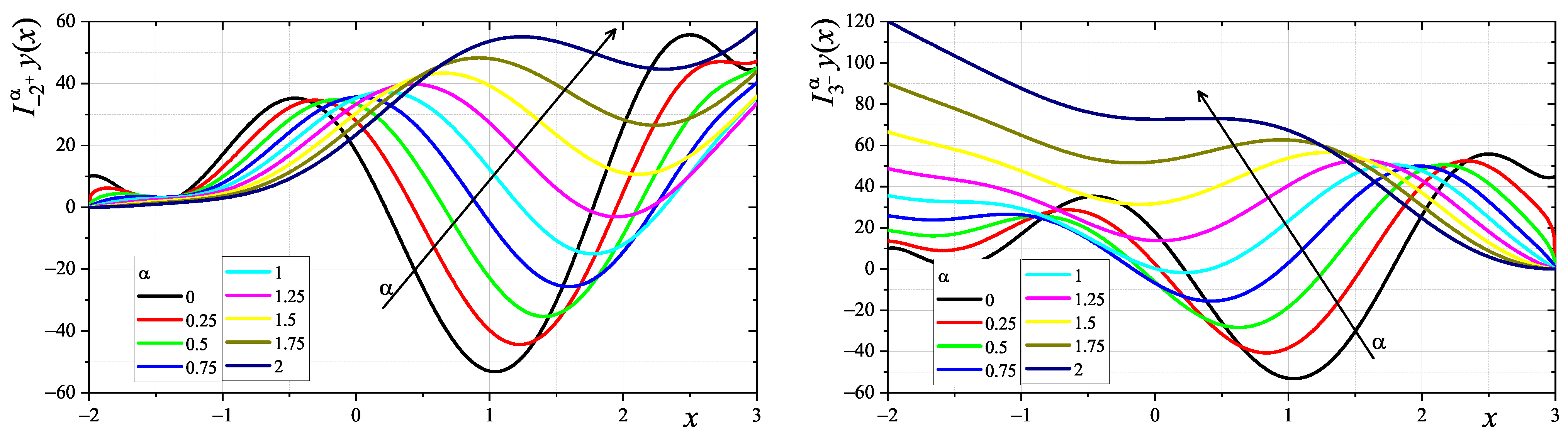
In Figure 1, the plots of the left- and right-sided fractional integrals $I_{-2^{+}}^{\alpha }y\left(x\right)$ and $I_{3^{-}}^{\alpha }y\left(x\right)$, (112) and (113), respectively, for $\alpha \in \{0,0.25,0.5,0.75,1,1.25,1.5,1.75,2\}$, are shown. The cases for $\alpha =0$ correspond to the plot of the function $y\left(x\right)$ (i.e., $I_{-2^{+}}^{0}y\left(x\right)=I_{3^{-}}^{0}y\left(x\right)=y\left(x\right)$), and, e.g., for $\alpha =1$: $I_{-2^{+}}^{1}y\left(x\right){|}_{x=3}=I_{3^{-}}^{1}y\left(x\right){|}_{x=-2}$, which is identical to the classical integration of the function $y\left(x\right)$ in the interval $[-2,3]$. 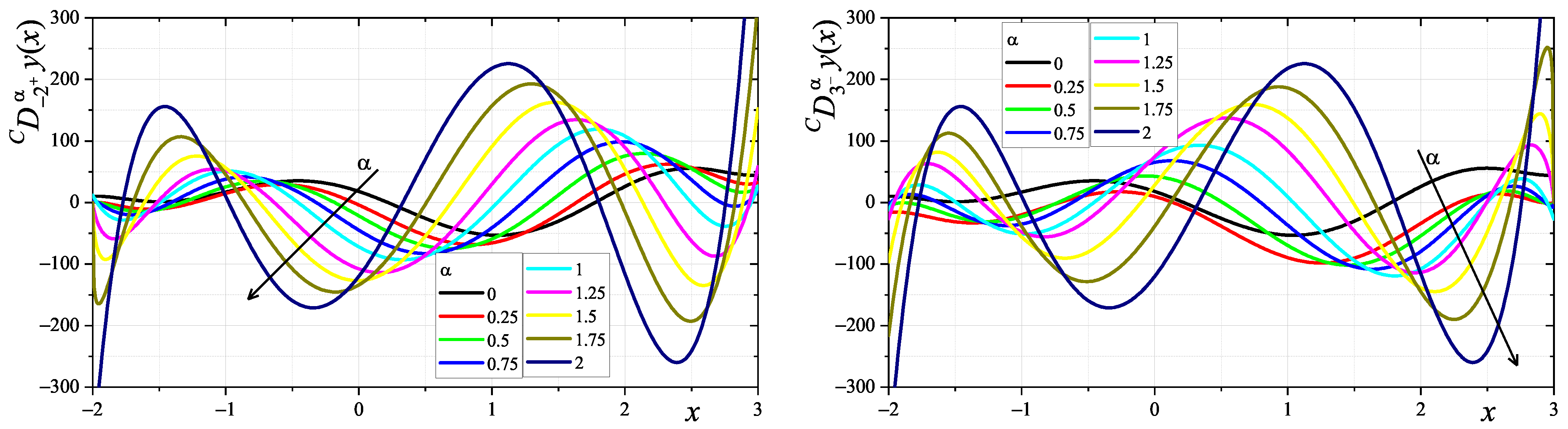Also, it can be seen that, for $\alpha >0$, $I_{-2^{+}}^{\alpha }y\left(x\right){|}_{x=-2}=0$ and $I_{3^{-}}^{\alpha }y\left(x\right){|}_{x=3}=0$ hold. In Figure 2, the plots related to the fractional derivatives ${ }^C{D}_{-2^{+}}^{\alpha }y\left(x\right)$ and ${ }^C{D}_{3^{-}}^{\alpha }y\left(x\right)$ are presented. As before, it can be noted that ${ }^C{D}_{-2^{+}}^{0}y\left(x\right)={ }^C{D}_{3^{-}}^{0}y\left(x\right)=y\left(x\right)$. On the other hand, for, e.g., $\alpha \in \{1,2\}$, ${ }^C{D}_{-2^{+}}^{1}y\left(x\right)=y^{\prime }\left(x\right)$, ${ }^C{D}_{-2^{+}}^{2}y\left(x\right)=y^{″}\left(x\right)$ and ${ }^C{D}_{3^{-}}^{1}y\left(x\right)=-y^{\prime }\left(x\right)$, ${ }^C{D}_{3^{-}}^{2}y\left(x\right)=y^{″}\left(x\right)$ occur. Moreover, for $\alpha \ne \mathbb{N}$, ${ }^C{D}_{-2^{+}}^{\alpha }y\left(x\right){|}_{x=-2}=0$ and ${ }^C{D}_{3^{-}}^{\alpha }y\left(x\right){|}_{x=3}=0$ occur.

Figure 1. Plots of integrals $I_{-2^{+}}^{\alpha }y\left(x\right)$ and $I_{3^{-}}^{\alpha }y\left(x\right)$ for function (104) and different orders of $\alpha$.

Figure 2. Plots of derivatives ${ }^C{D}_{-2^{+}}^{\alpha }y\left(x\right)$ and ${ }^C{D}_{3^{-}}^{\alpha }y\left(x\right)$ for function (104) and different orders of $\alpha$.

For each derived numerical scheme, the experimental order of convergence has been examined. Such tests make it possible to show the correctness and quality of these schemes based on sample calculations depending on, among other factors, the grid size N and order $\alpha$. If the exact/analytical solutions of fractional integrals and derivatives are known, then one can determine the computational error of the numerical scheme. In the case of $I_{a^{+}}^{\alpha }y\left(x\right)$, the error is as follows:

$$erro{r}_N={\left.I_{a^{+}}^{\alpha }y\left(x\right)\right|}_{x=x_R}-{\left.I_{a^{+}}^{\alpha }s\left(x\right)\right|}_{x=x_R},$$

(117)

where $I_{a^{+}}^{\alpha }s\left(x\right){|}_{x=x_R}$ denotes the approximate value of $I_{a^{+}}^{\alpha }y\left(x\right){|}_{x=x_R}$ that has been obtained on a grid of size N at a given data point $x_R$ by using the spline constructed by polynomials of degree p. The errors for the remaining operators are defined similarly. Based on the determined error values, the experimental order of convergence can be calculated using the following formula:

$$orde{r}_N={log}_2\frac{\left|erro{r}_{N/2}\right|}{\left|erro{r}_N\right|}.$$

(118)

In Table 1, the numerical errors (117) and the experimental orders of convergence (118) for the calculations of $I_{-2^{+}}^{\alpha }y\left(x\right){|}_{x=3}$ and $I_{3^{-}}^{\alpha }y\left(x\right){|}_{x=-2}$, for $\alpha \in \{0.25,0.5,0.75,1.0,1.25,1.5, 1.75,2.0\}$ and $N=125,250,500,1000,2000,4000$, using three kinds of splines are shown. Additionally, this table also provides the exact values of the calculated integrals. When $\alpha =1$, then the values of the left- and right-sided fractional integrals are identical. On the other hand, Table 2 contains the same set of data for the left- and right-sided Caputo fractional derivatives, but they are calculated for the same internal point $x=1$, i.e., ${ }^C{D}_{-2^{+}}^{\alpha }y\left(x\right){|}_{x=1}$ and ${ }^C{D}_{3^{-}}^{\alpha }y\left(x\right){|}_{x=1}$ (which corresponds to $x=x_R$, $R=N·3/5$). It is not possible to calculate fractional derivatives of order $\alpha >1$ in the case of the linear spline ($p=1$) or, analogously, $\alpha >3$ using the cubic spline and $\alpha >5$ using the quintic spline. Calculations for $\alpha >2$ have also been performed, but the results are omitted from both tables (due to lack of space).

Table 1. Results related to Riemann–Liouville fractional integrals.

$\mathit{\alpha }$	N	Left-Sided Riemann–Liouville Fractional Integral ${\left.{\mathit{I}}_{-2^{+}}^{\mathit{\alpha }}\mathit{y}\left(\mathit{x}\right)\right|}_{\mathit{x}=3}$						Right-Sided Riemann–Liouville Fractional Integral ${\left.{\mathit{I}}_{3^{-}}^{\mathit{\alpha }}\mathit{y}\left(\mathit{x}\right)\right|}_{\mathit{x}=-2}$
		Linear Spline		Cubic Spline		Quintic Spline		Linear Spline		Cubic Spline		Quintic Spline
		$\mathit{Error}$	$\mathit{Order}$	$\mathit{Error}$	$\mathit{Order}$	$\mathit{Error}$	$\mathit{Order}$	$\mathit{Error}$	$\mathit{Order}$	$\mathit{Error}$	$\mathit{Order}$	$\mathit{Error}$	$\mathit{Order}$
0.25	125	$-2.41675\times {10}^{-2}$	-	$1.04535\times {10}^{-5}$	-	$-5.69516\times {10}^{-9}$	-	$1.57811\times {10}^{-2}$	-	$6.80603\times {10}^{-6}$	-	$5.57276\times {10}^{-9}$	-
	250	$-6.86729\times {10}^{-3}$	1.815	$1.03230\times {10}^{-6}$	3.340	$-4.90212\times {10}^{-11}$	6.860	$4.49869\times {10}^{-3}$	1.811	$-7.49419\times {10}^{-7}$	3.183	$4.70124\times {10}^{-11}$	6.889
	500	$-1.88377\times {10}^{-3}$	1.866	$7.71362\times {10}^{-8}$	3.742	$-5.13316\times {10}^{-13}$	6.577	$1.23635\times {10}^{-3}$	1.863	$-5.75466\times {10}^{-8}$	3.703	$4.80667\times {10}^{-13}$	6.612
	1000	$-5.05293\times {10}^{-4}$	1.898	$5.27856\times {10}^{-9}$	3.869	$-6.50363\times {10}^{-15}$	6.302	$3.32029\times {10}^{-4}$	1.897	$-3.98006\times {10}^{-9}$	3.854	$5.97696\times {10}^{-15}$	6.329
	2000	$-1.33463\times {10}^{-4}$	1.921	$3.48367\times {10}^{-10}$	3.921	$-9.35790\times {10}^{-17}$	6.119	$8.77715\times {10}^{-5}$	1.919	$-2.64009\times {10}^{-10}$	3.914	$8.51330\times {10}^{-17}$	6.134
	4000	$-3.48577\times {10}^{-5}$	1.937	$2.25936\times {10}^{-11}$	3.947	$-1.43484\times {10}^{-18}$	6.027	$2.29381\times {10}^{-5}$	1.936	$-1.71712\times {10}^{-11}$	3.943	$1.30003\times {10}^{-18}$	6.033
0.50	125	$-1.63053\times {10}^{-2}$	-	$1.32582\times {10}^{-5}$	-	$-4.13856\times {10}^{-9}$	-	$1.01751\times {10}^{-2}$	-	$-8.06872\times {10}^{-6}$	-	$3.90697\times {10}^{-9}$	-
	250	$-4.39242\times {10}^{-3}$	1.892	$1.06143\times {10}^{-6}$	3.643	$-3.74296\times {10}^{-11}$	6.789	$2.75606\times {10}^3$	1.884	$-7.02674\times {10}^{-7}$	3.521	$3.37436\times {10}^{-11}$	6.855
	500	$-1.15081\times {10}^{-3}$	1.932	$7.24796\times {10}^{-8}$	3.872	$-4.38185\times {10}^{-13}$	6.416	$7.24321\times {10}^{-4}$	1.928	$-4.91460\times {10}^{-8}$	3.838	$3.79855\times {10}^{-13}$	6.473
	1000	$-2.96714\times {10}^{-4}$	1.956	$4.70229\times {10}^{-9}$	3.946	$-6.09673\times {10}^{-15}$	6.167	$1.87104\times {10}^{-4}$	1.953	$-3.21722\times {10}^{-9}$	3.933	$5.17726\times {10}^{-15}$	6.197
	2000	$-7.57427\times {10}^{-5}$	1.970	$2.99228\times {10}^{-10}$	3.974	$-9.18566\times {10}^{-17}$	6.053	$4.78204\times {10}^{-5}$	1.968	$-2.05529\times {10}^{-10}$	3.968	$7.74015\times {10}^{-17}$	6.064
	4000	$-1.92095\times {10}^{-5}$	1.979	$1.88860\times {10}^{-11}$	3.986	$-1.42490\times {10}^{-18}$	6.010	$1.21378\times {10}^{-5}$	1.978	$-1.29974\times {10}^{-11}$	3.983	$1.19807\times {10}^{-18}$	6.014
0.75	125	$-7.12111\times {10}^{-3}$	-	$9.97799\times {10}^{-6}$	-	$-2.05688\times {10}^{-9}$	-	$3.09092\times {10}^{-3}$	-	$-4.01756\times {10}^{-6}$	-	$1.70773\times {10}^{-9}$	-
	250	$-1.84844\times {10}^{-3}$	1.946	$7.14034\times {10}^{-7}$	3.805	$-2.10930\times {10}^{-11}$	6.608	$8.18172\times {10}^{-4}$	1.918	$-3.23904\times {10}^{-7}$	3.633	$1.56005\times {10}^{-11}$	6.774
	500	$-4.71369\times {10}^{-4}$	1.971	$4.65613\times {10}^{-8}$	3.939	$-2.78012\times {10}^{-13}$	6.245	$2.10729\times {10}^{-4}$	1.957	$-2.18291\times {10}^{-8}$	3.891	$1.91856\times {10}^{-13}$	6.345
	1000	$-1.19146\times {10}^{-4}$	1.984	$2.95257\times {10}^{-9}$	3.979	$-4.11580\times {10}^{-15}$	6.078	$5.35530\times {10}^{-5}$	1.976	$-1.39945\times {10}^{-9}$	3.963	$2.76659\times {10}^{-15}$	6.116
	2000	$-2.99742\times {10}^{-5}$	1.991	$1.85532\times {10}^{-10}$	3.992	$-6.34116\times {10}^{-17}$	6.020	$1.35137\times {10}^{-5}$	1.987	$-8.82904\times {10}^{-11}$	3.986	$4.23025\times {10}^{-17}$	6.031
	4000	$-7.52101\times {10}^{-6}$	1.995	$1.16215\times {10}^{-11}$	3.997	$-9.88375\times {10}^{-19}$	6.004	$3.39674\times {10}^{-6}$	1.992	$-5.53936\times {10}^{-12}$	3.994	$6.58293\times {10}^{-19}$	6.006
1.00	125	$-1.99648\times {10}^{-3}$	-	$3.40015\times {10}^{-6}$	-	$-2.42291\times {10}^{-10}$	-	$-1.99648\times {10}^{-3}$	-	$3.40015\times {10}^{-6}$	-	$-2.42291\times {10}^{-10}$	-
	250	$-4.99780\times {10}^{-4}$	1.998	$2.18102\times {10}^{-7}$	3.963	$-3.79766\times {10}^{-12}$	5.995	$-4.99780\times {10}^{-4}$	1.998	$2.18102\times {10}^{-7}$	3.963	$-3.79766\times {10}^{-12}$	5.995
	500	$-1.24986\times {10}^{-4}$	2.000	$1.37201\times {10}^{-8}$	3.991	$-5.94311\times {10}^{-14}$	5.998	$-1.24986\times {10}^{-4}$	2.000	$1.37201\times {10}^{-8}$	3.991	$-5.94311\times {10}^{-14}$	5.998
	1000	$-3.12491\times {10}^{-5}$	2.000	$8.58907\times {10}^{-10}$	3.998	$-9.29335\times {10}^{-16}$	5.999	$-3.12491\times {10}^{-5}$	2.000	$8.58907\times {10}^{-10}$	3.998	$-9.29335\times {10}^{-16}$	5.999
	2000	$-7.81245\times {10}^{-6}$	2.000	$5.37036\times {10}^{-11}$	3.999	$-1.45265\times {10}^{-17}$	5.999	$-7.81245\times {10}^{-6}$	2.000	$5.37036\times {10}^{-11}$	3.999	$-1.45265\times {10}^{-17}$	5.999
	4000	$-1.95312\times {10}^{-6}$	2.000	$3.35682\times {10}^{-12}$	4.000	$-2.27021\times {10}^{-19}$	6.000	$-1.95312\times {10}^{-6}$	2.000	$3.35682\times {10}^{-12}$	4.000	$-2.27021\times {10}^{-19}$	6.000
1.25	125	$2.94905\times {10}^{-5}$	-	$-5.04636\times {10}^{-6}$	-	$1.57623\times {10}^{-9}$	-	$-5.49391\times {10}^{-3}$	-	$1.31980\times {10}^{-5}$	-	$-2.21686\times {10}^{-9}$	-
	250	$8.21939\times {10}^{-6}$	1.843	$-3.63161\times {10}^{-7}$	3.797	$1.70155\times {10}^{-11}$	6.533	$-1.38221\times {10}^{-3}$	1.991	$8.83867\times {10}^{-7}$	3.900	$-2.70488\times {10}^{-11}$	6.357
	500	$2.18938\times {10}^{-6}$	1.909	$-2.35242\times {10}^{-8}$	3.948	$2.35877\times {10}^{-13}$	6.173	$-3.46277\times {10}^{-4}$	1.997	$5.62397\times {10}^{-8}$	3.974	$-3.92826\times {10}^{-13}$	6.106
	1000	$5.78985\times {10}^{-7}$	1.919	$-1.48421\times {10}^{-9}$	3.986	$3.57289\times {10}^{-15}$	6.045	$-8.66327\times {10}^{-5}$	1.999	$3.53152\times {10}^{-9}$	3.993	$-6.02658\times {10}^{-15}$	6.026
	2000	$1.51795\times {10}^{-7}$	1.931	$-9.29967\times {10}^{-11}$	3.996	$5.54430\times {10}^{-17}$	6.010	$-2.16640\times {10}^{-5}$	2.000	$2.20992\times {10}^{-10}$	3.998	$-9.37923\times {10}^{-17}$	6.006
	4000	$3.87101\times {10}^{-8}$	1.971	$-5.81622\times {10}^{-12}$	3.999	$8.65318\times {10}^{-19}$	6.002	$-5.41656\times {10}^{-6}$	2.000	$1.38165\times {10}^{-11}$	4.000	$-1.46461\times {10}^{-18}$	6.001
1.50	125	$6.47994\times {10}^{-4}$	-	$-1.48482\times {10}^{-5}$	-	$3.65727\times {10}^{-9}$	-	$-8.25052\times {10}^{-3}$	-	$2.50930\times {10}^{-5}$	-	$-4.47356\times {10}^{-9}$	−
	250	$1.71560\times {10}^{-4}$	1.917	$-1.02016\times {10}^{-6}$	3.863	$4.29330\times {10}^{-11}$	6.413	$-2.07231\times {10}^{-3}$	1.993	$1.67526\times {10}^{-6}$	3.905	$-5.57184\times {10}^{-11}$	6.327
	500	$4.35821\times {10}^{-5}$	1.977	$-6.52856\times {10}^{-8}$	3.966	$6.16466\times {10}^{-13}$	6.122	$-5.18747\times {10}^{-4}$	1.998	$1.06460\times {10}^{-7}$	3.976	$-8.16477\times {10}^{-13}$	6.093
	1000	$1.09467\times {10}^{-5}$	1.993	$-4.10500\times {10}^{-9}$	3.991	$9.43308\times {10}^{-15}$	6.030	$-1.29734\times {10}^{-4}$	1.999	$6.68202\times {10}^{-9}$	3.994	$-1.25601\times {10}^{-14}$	6.022
	2000	$2.74055\times {10}^{-6}$	1.998	$-2.56956\times {10}^{-10}$	3.998	$1.46728\times {10}^{-16}$	6.007	$-3.24368\times {10}^{-5}$	2.000	$4.18075\times {10}^{-10}$	3.998	$-1.95603\times {10}^{-16}$	6.005
	4000	$6.85440\times {10}^{-7}$	1.999	$-1.60660\times {10}^{-11}$	3.999	$2.29096\times {10}^{-18}$	6.001	$-8.10946\times {10}^{-6}$	2.000	$2.61368\times {10}^{-11}$	4.000	$-3.05474\times {10}^{-18}$	6.001
1.75	125	$1.46683\times {10}^{-3}$	-	$-2.58868\times {10}^{-5}$	-	$6.11752\times {10}^{-9}$	-	$-1.07883\times {10}^{-2}$	-	$3.90746\times {10}^{-5}$	-	$-7.12572\times {10}^{-9}$	-
	250	$3.76033\times {10}^{-4}$	1.964	$-1.75690\times {10}^{-6}$	3.881	$7.43135\times {10}^{-11}$	6.363	$-2.70816\times {10}^{-3}$	1.994	$2.60169\times {10}^{-6}$	3.909	$-9.01099\times {10}^{-11}$	6.305
	500	$9.46089\times {10}^{-5}$	1.991	$-1.12075\times {10}^{-7}$	3.970	$1.08058\times {10}^{-12}$	6.104	$-6.77746\times {10}^{-4}$	1.998	$1.65199\times {10}^{-7}$	3.977	$-1.32774\times {10}^{-12}$	6.085
	1000	$2.36910\times {10}^{-5}$	1.998	$-7.04090\times {10}^{-9}$	3.993	$1.65911\times {10}^{-14}$	6.025	$-1.69481\times {10}^{-4}$	2.000	$1.03663\times {10}^{-8}$	3.994	$-2.04555\times {10}^{-14}$	6.020
	2000	$5.92525\times {10}^{-6}$	1.999	$-4.40629\times {10}^{-10}$	3.998	$2.58264\times {10}^{-16}$	6.005	$-4.23732\times {10}^{-5}$	2.000	$6.48547\times {10}^{-10}$	3.999	$-3.18667\times {10}^{-16}$	6.004
	4000	$1.48148\times {10}^{-6}$	2.000	$-2.75483\times {10}^{-11}$	4.000	$4.03294\times {10}^{-18}$	6.001	$-1.05935\times {10}^{-5}$	2.000	$4.05444\times {10}^{-11}$	4.000	$-4.97689\times {10}^{-18}$	6.001
2.00	125	$3.27639\times {10}^{-3}$	-	$-3.81492\times {10}^{-5}$	-	$8.97159\times {10}^{-9}$	-	$-1.32588\times {10}^{-2}$	-	$5.51500\times {10}^{-5}$	-	$-1.01830\times {10}^{-8}$	-
	250	$8.29774\times {10}^{-4}$	1.981	$-2.57717\times {10}^{-6}$	3.888	$1.10742\times {10}^{-10}$	6.340	$-3.32867\times {10}^{-3}$	1.994	$3.66768\times {10}^{-6}$	3.910	$-1.29731\times {10}^{-10}$	6.295
	500	$2.08111\times {10}^{-4}$	1.995	$-1.64209\times {10}^{-7}$	3.972	$1.61914\times {10}^{-12}$	6.096	$-8.33042\times {10}^{-4}$	1.998	$2.32809\times {10}^{-7}$	3.978	$-1.91630\times {10}^{-12}$	6.081
	1000	$5.20694\times {10}^{-5}$	1.999	$-1.03130\times {10}^{-8}$	3.993	$2.48952\times {10}^{-14}$	6.023	$-2.08315\times {10}^{-4}$	2.000	$1.46076\times {10}^{-8}$	3.994	$-2.95419\times {10}^{-14}$	6.019
	2000	$1.30200\times {10}^{-5}$	2.000	$-6.45352\times {10}^{-10}$	3.998	$3.87650\times {10}^{-16}$	6.005	$-5.20822\times {10}^{-5}$	2.000	$9.13870\times {10}^{-10}$	3.999	$-4.60283\times {10}^{-16}$	6.004
	4000	$3.25515\times {10}^{-6}$	2.000	$-4.03469\times {10}^{-11}$	4.000	$6.05369\times {10}^{-18}$	6.001	$-1.30208\times {10}^{-5}$	2.000	$5.71310\times {10}^{-11}$	4.000	$-7.18879\times {10}^{-18}$	6.001
$\alpha$		Analytical values of ${\left.I_{-2^{+}}^{\alpha }y\left(x\right)\right|}_{x=3}$ calculated using (112)						Analytical values of ${\left.I_{3^{-}}^{\alpha }y\left(x\right)\right|}_{x=-2}$ calculated using (113)
0.25		47.231705520698452904374875899367						13.548112447243133497964663253209
0.50		44.959314436662925135432890756581						18.729546832067732625877247675307
0.75		40.207326196989011686391620773830						25.873320468390417138456826053977
1.00		35.565476190476190476190476190354						35.565476190476190476190476190594
1.25		33.495522685430899963086433632447						48.724522699297574882594335266746
1.50		35.883958339131400674417388236684						66.494895409838463421125458683182
1.75		43.817498620131802938994234913290						90.037106096993660710700647449116
2.00		57.539682539682539682539682539625						120.287698412698412698412698412756

Table 2. Results related to Caputo fractional derivatives.

$\mathit{\alpha }$	N	Left-Sided Caputo Fractional Derivative ${\left.{ }^{\mathit{C}}{\mathit{D}}_{-2^{+}}^{\mathit{\alpha }}\mathit{y}\left(\mathit{x}\right)\right|}_{\mathit{x}=1}$						Right-Sided Caputo Fractional Derivative ${\left.{ }^{\mathit{C}}{\mathit{D}}_{3^{-}}^{\mathit{\alpha }}\mathit{y}\left(\mathit{x}\right)\right|}_{\mathit{x}=1}$
		Linear Spline		Cubic Spline		Quintic Spline		Linear Spline		Cubic Spline		Quintic Spline
		$\mathit{Error}$	$\mathit{Order}$	$\mathit{Error}$	$\mathit{Order}$	$\mathit{Error}$	$\mathit{Order}$	$\mathit{Error}$	$\mathit{Order}$	$\mathit{Error}$	$\mathit{Order}$	$\mathit{Error}$	$\mathit{Order}$
0.25	125	$7.84165\times {10}^{-2}$	-	$6.98882\times {10}^{-6}$	-	$5.55910\times {10}^{-10}$	-	$8.46350\times {10}^{-2}$	-	$6.83433\times {10}^{-6}$	-	$1.40106\times {10}^{-9}$	-
	250	$2.49924\times {10}^{-2}$	1.650	$5.68971\times {10}^{-7}$	3.619	$1.29900\times {10}^{-11}$	5.419	$2.65102\times {10}^{-2}$	1.675	$5.47833\times {10}^{-7}$	3.641	$2.49565\times {10}^{-11}$	5.811
	500	$7.84618\times {10}^{-3}$	1.671	$4.51782\times {10}^{-8}$	3.655	$2.76433\times {10}^{-13}$	5.554	$8.22011\times {10}^{-3}$	1.689	$4.35584\times {10}^{-8}$	3.653	$4.56394\times {10}^{-13}$	5.773
	1000	$2.43616\times {10}^{-3}$	1.687	$3.53309\times {10}^{-9}$	3.677	$5.64871\times {10}^{-15}$	5.613	$2.52882\times {10}^{-3}$	1.701	$3.42284\times {10}^{-9}$	3.670	$8.41279\times {10}^{-15}$	5.762
	2000	$7.50076\times {10}^{-4}$	1.700	$2.73386\times {10}^{-10}$	3.692	$1.12730\times {10}^{-16}$	5.647	$7.73116\times {10}^{-4}$	1.710	$2.66193\times {10}^{-10}$	3.685	$1.55540\times {10}^{-16}$	5.757
	4000	$2.29439\times {10}^{-4}$	1.709	$2.09882\times {10}^{-11}$	3.703	$2.21425\times {10}^{-18}$	5.670	$2.35181\times {10}^{-4}$	1.717	$2.05280\times {10}^{-11}$	3.697	$2.87991\times {10}^{-18}$	5.755
0.50	125	$3.71896\times {10}^{-1}$	-	$2.50923\times {10}^{-5}$	-	$2.45199\times {10}^{-9}$	-	$3.87777\times {10}^{-1}$	-	$2.74995\times {10}^{-5}$	-	$4.13307\times {10}^{-9}$	-
	250	$1.35444\times {10}^{-1}$	1.457	$2.35615\times {10}^{-6}$	3.413	$6.21460\times {10}^{-11}$	5.302	$1.39254\times {10}^{-1}$	1.478	$2.47549\times {10}^{-6}$	3.474	$8.55722\times {10}^{-11}$	5.594
	500	$4.88554\times {10}^{-2}$	1.471	$2.16262\times {10}^{-7}$	3.446	$1.48114\times {10}^{-12}$	5.391	$4.97795\times {10}^{-2}$	1.484	$2.22544\times {10}^{-7}$	3.476	$1.82243\times {10}^{-12}$	5.553
	1000	$1.75120\times {10}^{-2}$	1.480	$1.95907\times {10}^{-8}$	3.465	$3.42745\times {10}^{-14}$	5.433	$1.77380\times {10}^{-2}$	1.489	$1.99345\times {10}^{-8}$	3.481	$3.93594\times {10}^{-14}$	5.533
	2000	$6.25069\times {10}^{-3}$	1.486	$1.76026\times {10}^{-9}$	3.476	$7.80135\times {10}^{-16}$	5.457	$6.30629\times {10}^{-3}$	1.492	$1.77965\times {10}^{-9}$	3.486	$8.56945\times {10}^{-16}$	5.521
	4000	$2.22468\times {10}^{-3}$	1.490	$1.57333\times {10}^{-10}$	3.484	$1.75798\times {10}^{-17}$	5.472	$2.23842\times {10}^{-3}$	1.494	$1.58453\times {10}^{-10}$	3.489	$1.87511\times {10}^{-17}$	5.514
0.75	125	1.34310	-	$5.19229\times {10}^{-5}$	-	$4.97092\times {10}^{-9}$	-	1.37524	-	$6.14400\times {10}^{-5}$	-	$8.28007\times {10}^{-9}$	-
	250	$5.71054\times {10}^{-1}$	1.234	$5.78626\times {10}^{-6}$	3.166	$1.51641\times {10}^{-10}$	5.035	$5.78725\times {10}^{-1}$	1.249	$6.31959\times {10}^{-6}$	3.281	$1.98166\times {10}^{-10}$	5.385
	500	$2.41617\times {10}^{-1}$	1.241	$6.27234\times {10}^{-7}$	3.206	$4.27870\times {10}^{-12}$	5.147	$2.43458\times {10}^{-1}$	1.249	$6.57509\times {10}^{-7}$	3.265	$4.94268\times {10}^{-12}$	5.325
	1000	$1.01956\times {10}^{-1}$	1.245	$6.70419\times {10}^{-8}$	3.226	$1.16612\times {10}^{-13}$	5.197	$1.02400\times {10}^{-1}$	1.249	$6.87761\times {10}^{-8}$	3.257	$1.26179\times {10}^{-13}$	5.292
	2000	$4.29571\times {10}^{-2}$	1.247	$7.11235\times {10}^{-9}$	3.237	$3.12427\times {10}^{-15}$	5.222	$4.30647\times {10}^{-2}$	1.250	$7.21248\times {10}^{-9}$	3.253	$3.26321\times {10}^{-15}$	5.273
	4000	$1.80834\times {10}^{-2}$	1.248	$7.51469\times {10}^{-10}$	3.243	$8.29667\times {10}^{-17}$	5.235	$1.81095\times {10}^{-2}$	1.250	$7.57293\times {10}^{-10}$	3.252	$8.49994\times {10}^{-17}$	5.263
1.00	125	$-4.38955$	-	$-1.36670\times {10}^{-5}$	-	$-4.09600\times {10}^{-9}$	-	4.38955	-	$1.36670\times {10}^{-5}$	-	$4.09600\times {10}^{-9}$	-
	250	$-2.18769$	1.005	$-8.53547\times {10}^{-7}$	4.001	$-6.40000\times {10}^{-11}$	6.000	2.18769	1.005	$8.53547\times {10}^{-7}$	4.001	$6.40000\times {10}^{-11}$	6.000
	500	$-1.09196$	1.002	$-5.33367\times {10}^{-8}$	4.000	$-1.00000\times {10}^{-12}$	6.000	1.09196	1.002	$5.33367\times {10}^{-8}$	4.000	$1.00000\times {10}^{-12}$	6.000
	1000	$-5.4549\times {10}^{-1}$	1.001	$-3.33339\times {10}^{-9}$	4.000	$-1.56250\times {10}^{-14}$	6.000	$5.45495\times {10}^{-1}$	1.001	$3.33339\times {10}^{-9}$	4.000	$1.56250\times {10}^{-14}$	6.000
	2000	$-2.72624\times {10}^{-1}$	1.001	$-2.08334\times {10}^{-10}$	4.000	$-2.44141\times {10}^{-16}$	6.000	$2.72624\times {10}^{-1}$	1.001	$2.08334\times {10}^{-10}$	4.000	$2.44141\times {10}^{-16}$	6.000
	4000	$-1.36281\times {10}^{-1}$	1.000	$-1.30208\times {10}^{-11}$	4.000	$-3.81470\times {10}^{-18}$	6.000	$1.36281\times {10}^{-1}$	1.000	$1.30208\times {10}^{-11}$	4.000	$3.81470\times {10}^{-18}$	6.000
1.25	125	-	-	$-8.36678\times {10}^{-4}$	-	$-9.64146\times {10}^{-8}$	-	-	-	$-7.65038\times {10}^{-4}$	-	$-7.39989\times {10}^{-8}$	-
	250	-	-	$-1.21870\times {10}^{-4}$	2.779	$-3.37429\times {10}^{-9}$	4.837	-	-	$-1.16655\times {10}^{-4}$	2.713	$-2.96113\times {10}^{-9}$	4.643
	500	-	-	$-1.79335\times {10}^{-5}$	2.765	$-1.21552\times {10}^{-10}$	4.795	-	-	$-1.75527\times {10}^{-5}$	2.732	$-1.13927\times {10}^{-10}$	4.700
	1000	-	-	$-2.65243\times {10}^{-6}$	2.757	$-4.44624\times {10}^{-12}$	4.773	-	-	$-2.62455\times {10}^{-6}$	2.742	$-4.30538\times {10}^{-12}$	4.726
	2000	-	-	$-3.93299\times {10}^{-7}$	2.754	$-1.63924\times {10}^{-13}$	4.761	-	-	$-3.91253\times {10}^{-7}$	2.746	$-1.61319\times {10}^{-13}$	4.738
	4000	-	-	$-5.83913\times {10}^{-8}$	2.752	$-6.06763\times {10}^{-15}$	4.756	-	-	$-5.82409\times {10}^{-8}$	2.748	$-6.01943\times {10}^{-15}$	4.744
1.50	125	-	-	$-7.72196\times {10}^{-3}$	-	$-5.90738\times {10}^{-7}$	-	-	-	$-5.50777\times {10}^{-3}$	-	$-5.35105\times {10}^{-7}$	-
	250	-	-	$-1.12814\times {10}^{-3}$	2.775	$-2.54920\times {10}^{-8}$	4.534	-	-	$-9.81527\times {10}^{-4}$	2.488	$-2.42676\times {10}^{-8}$	4.463
	500	-	-	$-1.83845\times {10}^{-4}$	2.617	$-1.11306\times {10}^{-9}$	4.517	-	-	$-1.74190\times {10}^{-4}$	2.494	$-1.08608\times {10}^{-9}$	4.482
	1000	-	-	$-3.14907\times {10}^{-5}$	2.545	$-4.88926\times {10}^{-11}$	4.509	-	-	$-3.08513\times {10}^{-5}$	2.497	$-4.82977\times {10}^{-11}$	4.491
	2000	-	-	$-5.50177\times {10}^{-6}$	2.517	$-2.15419\times {10}^{-12}$	4.504	-	-	$-5.45886\times {10}^{-6}$	2.499	$-2.14107\times {10}^{-12}$	4.496
	4000	-	-	$-9.68377\times {10}^{-7}$	2.506	$-9.50577\times {10}^{-14}$	4.502	-	-	$-9.65442\times {10}^{-7}$	2.499	$-9.47679\times {10}^{-14}$	4.498
1.75	125	-	-	$-2.90741\times {10}^{-2}$	-	$-3.04121\times {10}^{-6}$	-	-	-	$-2.68499\times {10}^{-2}$	-	$-2.10060\times {10}^{-6}$	-
	250	-	-	$-5.98591\times {10}^{-3}$	2.280	$-1.45340\times {10}^{-7}$	4.387	-	-	$-5.83124\times {10}^{-3}$	2.203	$-1.29579\times {10}^{-7}$	4.019
	500	-	-	$-1.24961\times {10}^{-3}$	2.260	$-7.39805\times {10}^{-9}$	4.296	-	-	$-1.23857\times {10}^{-3}$	2.235	$-7.12385\times {10}^{-9}$	4.185
	1000	-	-	$-2.62077\times {10}^{-4}$	2.253	$-3.84688\times {10}^{-10}$	4.265	-	-	$-2.61252\times {10}^{-4}$	2.245	$-3.79670\times {10}^{-10}$	4.230
	2000	-	-	$-5.50488\times {10}^{-5}$	2.251	$-2.01436\times {10}^{-11}$	4.255	-	-	$-5.49833\times {10}^{-5}$	2.248	$-2.00459\times {10}^{-11}$	4.243
	4000	-	-	$-1.15690\times {10}^{-5}$	2.250	$-1.05726\times {10}^{-12}$	4.252	-	-	$-1.15634\times {10}^{-5}$	2.249	$-1.05522\times {10}^{-12}$	4.248
2.00	125	-	-	$-1.21620\times {10}^{-1}$	-	$-1.02400\times {10}^{-5}$	-	-	-	$-1.21620\times {10}^{-1}$	-	$-1.02400\times {10}^{-5}$	-
	250	-	-	$-3.04013\times {10}^{-2}$	2.000	$-6.40000\times {10}^{-7}$	4.000	-	-	$-3.04013\times {10}^{-2}$	2.000	$-6.40000\times {10}^{-7}$	4.000
	500	-	-	$-7.60008\times {10}^{-3}$	2.000	$-4.00000\times {10}^{-8}$	4.000	-	-	$-7.60008\times {10}^{-3}$	2.000	$-4.00000\times {10}^{-8}$	4.000
	1000	-	-	$-1.90001\times {10}^{-3}$	2.000	$-2.50000\times {10}^{-9}$	4.000	-	-	$-1.90001\times {10}^{-3}$	2.000	$-2.50000\times {10}^{-9}$	4.000
	2000	-	-	$-4.75000\times {10}^{-4}$	2.000	$-1.56250\times {10}^{-10}$	4.000	-	-	$-4.75000\times {10}^{-4}$	2.000	$-1.56250\times {10}^{-9}$	4.000
	4000	-	-	$-1.18750\times {10}^{-4}$	2.000	$-9.76562\times {10}^{-12}$	4.000	-	-	$1.18750\times {10}^{-4}$	2.000	$-9.76562\times {10}^{-12}$	4.000
$\alpha$		Analytical values of ${\left.{ }^C{D}_{-2^{+}}^{\alpha }y\left(x\right)\right|}_{x=1}$ calculated using (114)						Analytical values of ${\left.{ }^C{D}_{3^{-}}^{\alpha }y\left(x\right)\right|}_{x=1}$ calculated using (115)
0.25		−65.695900671274686868366861533907						−89.684783620466897066778246346165
0.50		−59.331281245578144164503719955315						−69.874990609212284201036182289303
0.75		−41.076691104317504450100614025998						−36.962637833302769019389855861950
1.00		−9.000000000000000000000000000000						9.000000000000000000000000000000
1.25		29.666322127181412268762909469963						83.928086254218424666184559890907
1.50		90.928292916416640368366975213304						137.009559059007698495559102959142
1.75		156.918453309420023096180630755186						186.059723786166269221860579765927
2.00		218.000000000000000000000000000000						218.000000000000000000000000000000

Remarks on numerical calculations: All calculations were performed with quadruple floating-point precision. The numerical algorithms were implemented in C++11 using the quadmath library and compiled in the GCC (MinGW-w64) compiler. The mentioned library enables the use of the 128-bit floating-point type _ _float128 for real variables and allows calculations with 34 significant decimal digits. This is mainly visible in the case of calculations for $N=4000$ using the quintic spline, where the error values are at the level of ${10}^{-18}$. When the single or double floating-point precision types were used, then the calculations (especially regarding the order of convergence) were imprecise.

In the second example, for all fractional operators, the integrand function $y\left(x\right)$ is of the form

$$y\left(x\right)=\frac{sin\left({\displaystyle \frac{3\pi }{2}}\left(x-3\right)\right)}{{\displaystyle \frac{3\pi }{2}}\left(x-3\right)}.$$

(119)

Here, in the considered interval $[a,b]$, for $a=1$ and $b=5$, this function is symmetric about the midpoint of the interval ($(a+b)/2=3$), i.e., $y\left(x\right)=y(a+b-x)$, and moreover, $y\left(a\right)=y\left(b\right)=0$. So far, the analytical forms of fractional integrals and derivatives for the above function $y\left(x\right)$ are not known. In Figure 3, the plots of the fractional integrals $I_{1^{+}}^{\alpha }y\left(x\right)$ and $I_{5^{-}}^{\alpha }y\left(x\right)$, for $\alpha \in \{0,0.25,0.5,0.75,1,1.25,1.5,1.75,2\}$, are shown. To create these plots, numerical values calculated by the method using the quintic spline for the grid size $N=1000$ were used. The plots of the integrand function $y\left(x\right)$ are represented by the case for $\alpha =0$. As can be seen in the presented plots of the left- and right-sided fractional integrals of the symmetric function about the midpoint of the interval $[a,b]$, both solutions are symmetrical; i.e., the following relationship occurs:

$${\left.I_{a^{+}}^{\alpha }y\left(x\right)\right|}_{x=u}={\left.I_{b^{-}}^{\alpha }y\left(x\right)\right|}_{x=a+b-u},\mathrm{for}u\in \left[a,b\right],$$

(120)

or in the discrete form as $I_{a^{+}}^{\alpha }y\left(x\right){|}_{x=x_R}=I_{b^{-}}^{\alpha }y\left(x\right){|}_{x=x_{N-R}}$, for $R=0,\dots ,N$. By analogy, in Figure 4, the plots related to the fractional derivatives ${ }^C{D}_{1^{+}}^{\alpha }y\left(x\right)$ and ${ }^C{D}_{5^{-}}^{\alpha }y\left(x\right)$ are shown. Here, one can also notice the presence of symmetry, i.e.,

$${\left.{ }^C{D}_{a^{+}}^{\alpha }y\left(x\right)\right|}_{x=u}={\left.{ }^C{D}_{b^{-}}^{\alpha }y\left(x\right)\right|}_{x=a+b-u},\mathrm{for}u\in \left[a,b\right].$$

(121)

Figure 3. Plots of integrals $I_{1^{+}}^{\alpha }y\left(x\right)$ and $I_{5^{-}}^{\alpha }y\left(x\right)$ for function (119) and different orders of $\alpha$.

Figure 4. Plots of derivatives ${ }^C{D}_{1^{+}}^{\alpha }y\left(x\right)$ and ${ }^C{D}_{5^{-}}^{\alpha }y\left(x\right)$ for function (119) and different orders of $\alpha$.

Moreover, for $\alpha \in \{1,2\}$, one can see that ${ }^C{D}_{1^{+}}^{1}y\left(x\right)=-{ }^C{D}_{5^{-}}^{1}y\left(x\right)=y^{\prime }\left(x\right)$ and ${ }^C{D}_{1^{+}}^{2}y\left(x\right)={ }^C{D}_{5^{-}}^{2}y\left(x\right)=y^{″}\left(x\right)$.

5. Conclusions

Numerical schemes for evaluating the left- and right-sided integrals and derivatives of fractional order based on the interpolation of the integrand function by splines have been derived. The primary purpose of this work was to research the application of the quintic spline, but two remaining lower-degree splines (linear and cubic) were used for comparison purposes. The quintic spline creates a curve that appears to be seamless and has smooth characteristics compared to the cubic spline. Generally, if the spline is built with higher degrees of polynomials, then the curve is smoother and the approximation of the function by such a spline has smaller differences.

The analysis of the sample results presented in two tables (and others, but not shown in this paper) allows the conclusion that the absolute values of numerical errors tend to 0 as the grid size N increases in all cases, which means that the numerical results are in good agreement with the exact analytical solutions. Moreover, one can observe that as N increases, the values of the experimental order of convergence are stabilized and take the specified values: see Table 3. It should be pointed out that the numerical schemes that use the quintic spline give a higher order of convergence than other schemes. For example, the scheme of sixth order means that by doubling the number of nodes in the grid, the calculation errors decrease by $2^6=64$ times, which significantly affects the quality of the calculations compared to other schemes. Furthermore, it can be stated that the experimental orders of convergence are consistent with analytical estimates (97) and (103).

Table 3. Experimental orders of convergence of numerical schemes that use different kinds of splines.

Kind of Spline	Experimental Order of Convergence
	Riemann–Liouville Fractional Integrals	Caputo Fractional Derivatives
linear spline ($p=1$)	2	$2-\alpha$ (for $\alpha \le 1$)
cubic spline ($p=3$)	4	$4-\alpha$ (for $\alpha \le 3$)
quintic spline ($p=5$)	6	$6-\alpha$ (for $\alpha \le 5$)

In the case of schemes that use the quintic and cubic splines, a system of linear equations (in order to determine the spline interpolation coefficients) needs to be solved. From the computational point of view, such a procedure can be computationally time-consuming, which may indicate a disadvantage of these schemes. But one can use the Thomas algorithm of linear complexity to solve the block tridiagonal system of equations. Moreover, the global approximation properties of the cubic and quintic splines mean that the polynomial coefficients in each segment of any spline depend on all data points. The perturbation of one arbitrary data point or a slight change in the values of the endpoint conditions affect the construction of the whole spline $s\left(x\right)$. Hence, it is worth taking more precise numerical values of the endpoint conditions or, preferably, taking their exact values in the considered systems of linear equations.

Summing up, the developed approximation methods for the considered fractional operators that use the quintic spline interpolation seem to be correct, and they have a qualitative advantage over methods that use other splines of lower degrees. This confirms the efficiency and applicability of the derived methods. In future works, it will be worth focusing on applications of the developed numerical methods to solve differential or integral equations.