
An Adaptive Two-Class Teaching-Learning-Based Optimization for Energy-Efficient Hybrid Flow Shop Scheduling Problems with Additional Resources

Abstract
1. Introduction
- An EHFSP with additional resources is considered.
- An adaptive two-class teaching-learning-based optimization (ATLBO) is presented to minimize the makespan and total energy consumption simultaneously. To produce high quality solutions, a teacher phase with teacher self-learning and teacher training are presented and an adaptive learner phase is reported which uses the quality of two classes to decide adaptively the learner phase or the reinforcement search of the temporary solution set. An adaptive formation of classes is also performed.
- The performance of the ATLBO is tested through a number of experiments. The effectiveness of the new strategies of the ATLBO is validated and the search advantages of the ATLBO for solving the EHFSP with additional resources is also demonstrated.
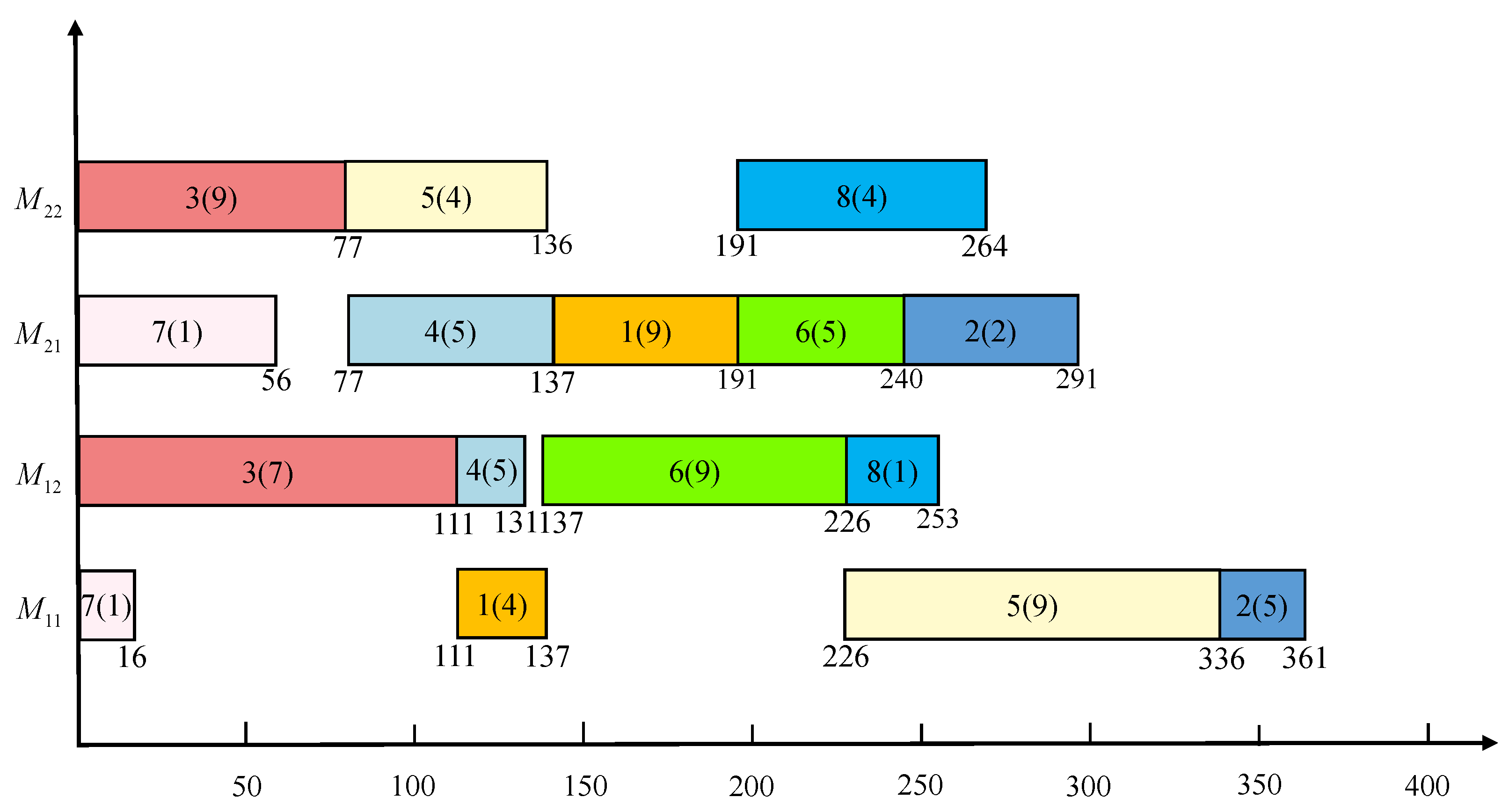
2. Problem Description
3. ATLBO for EHFSP with Additional Resources
3.1. Initialization and Formation of Two Classes
3.2. Teacher Phase
3.3. Adaptive Learner Phase
3.4. Algorithm Description
4. Computational Experiments
4.1. Test Instances, Metrics, and Comparative Algorithms
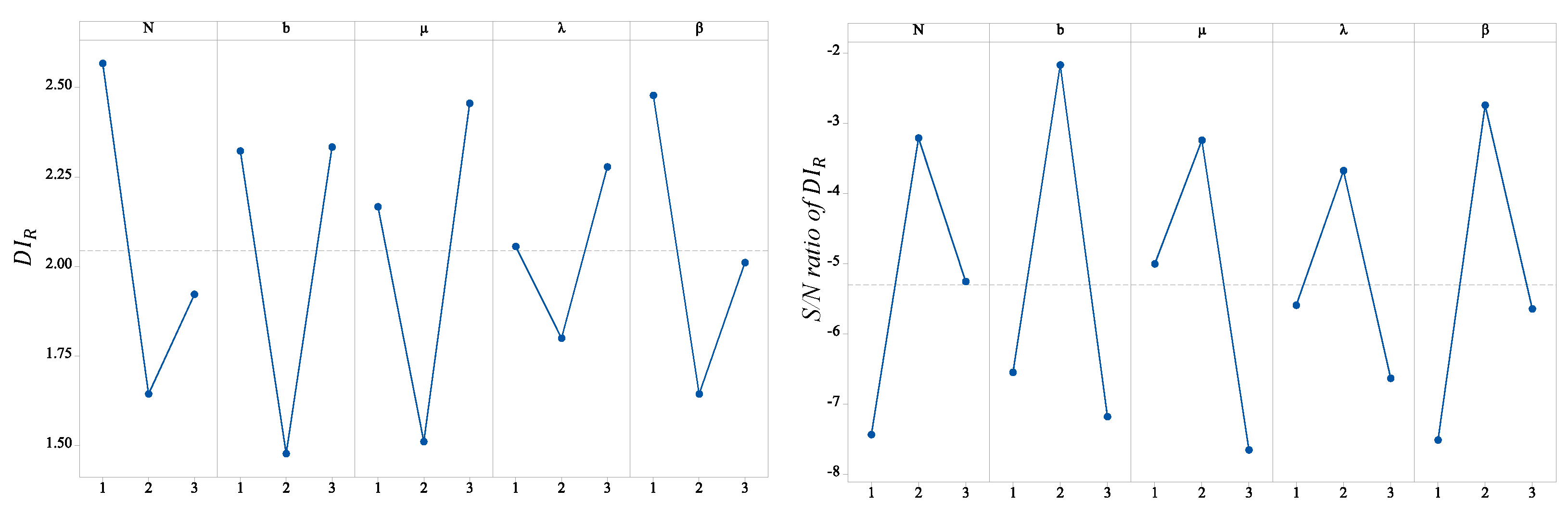
4.2. Parameter Settings
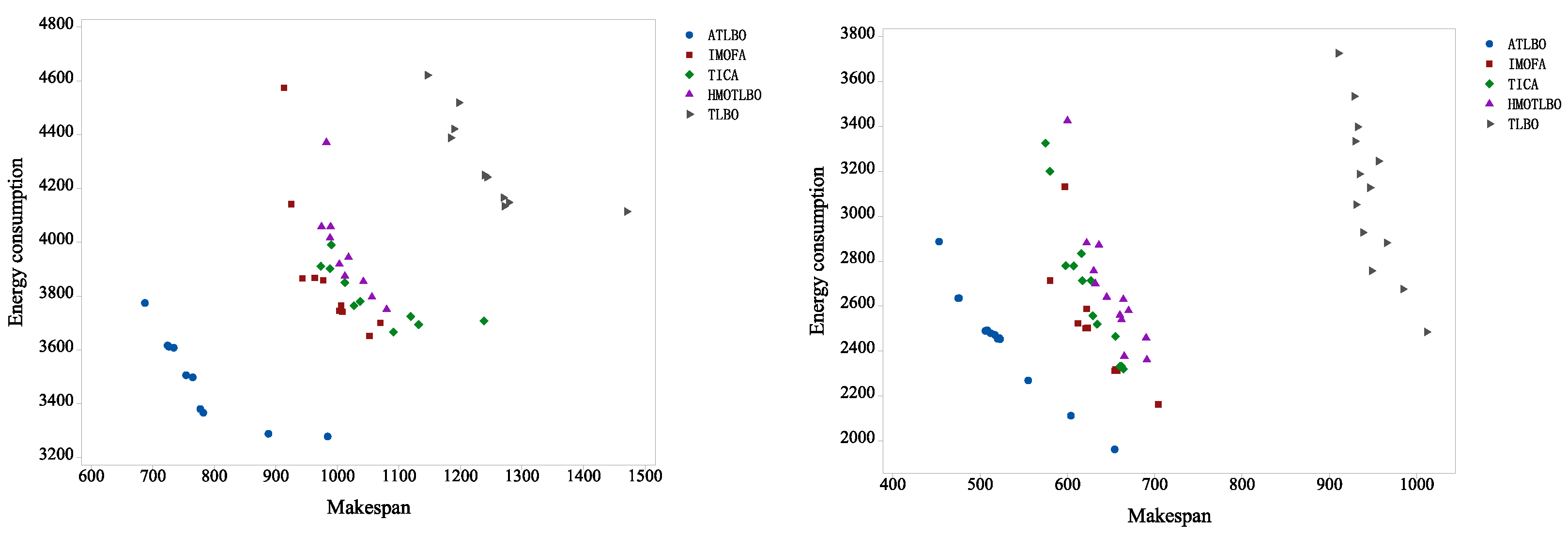
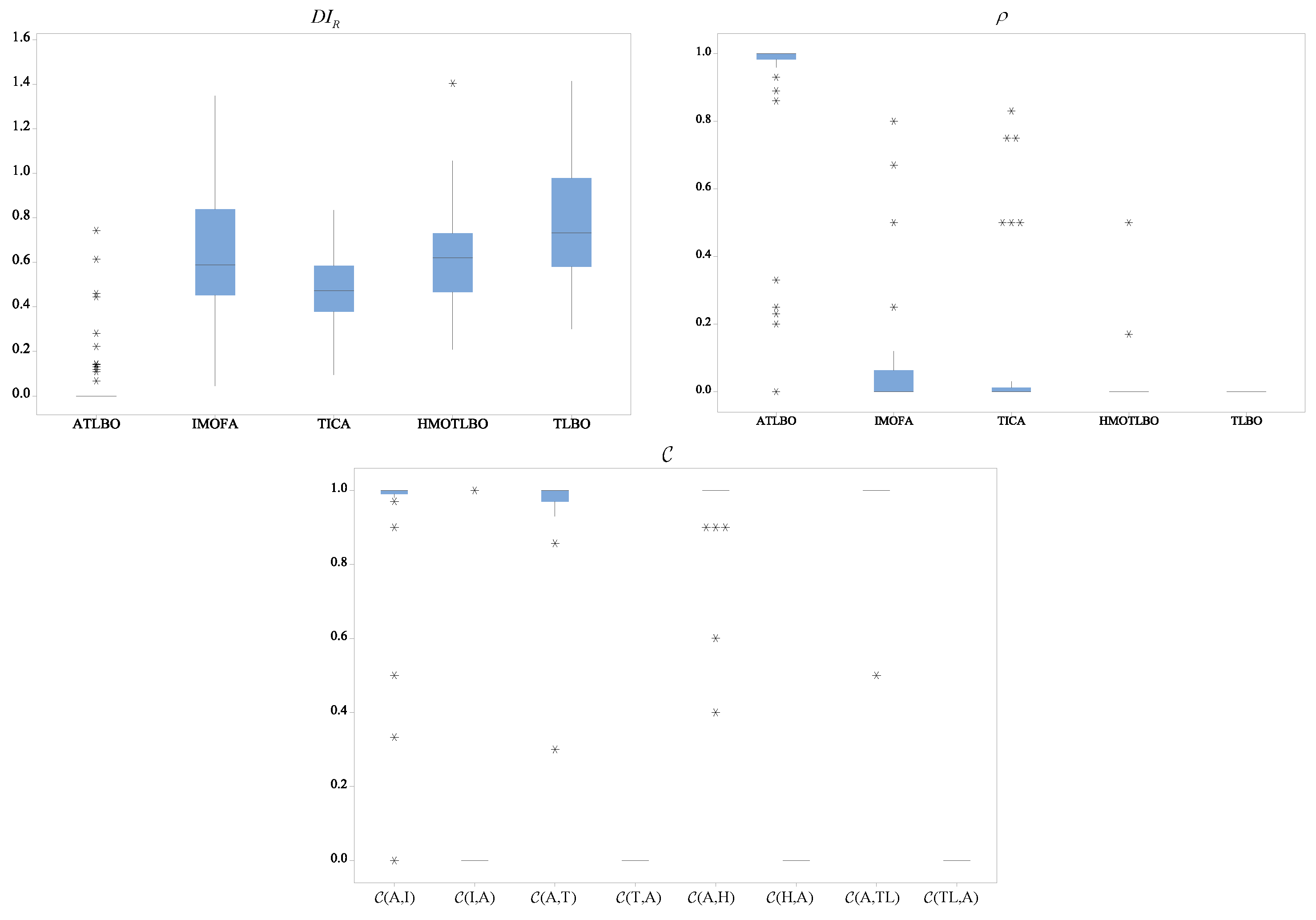
4.3. Results and Discussion
5. Conclusions
Author Contributions
Funding
Institutional Review Board Statement
Informed Consent Statement
Data Availability Statement
Conflicts of Interest
Nomenclature
| the number of machines at stage l | |
| the k-th machines at stage l | |
| the processed job needs units of the additional resource on | |
| the total number available of additional resources at stage l | |
| the energy consumption per unit time of processing mode on | |
| the energy consumption per unit time of idle mode on | |
| the completion time of job | |
| the maximum completion time of all jobs | |
| the total energy consumption | |
| decision variable, if job is processed on at time t, = 1; | |
| otherwise = 0 | |
| decision variable, if machine is free at time t, = 1; | |
| otherwise = 0 | |
| the evaluation index of class |
References
- Ruiz, R.; Vázquez-Rodríguez, J.A. The hybrid flow shop scheduling problem. Eur. J. Oper. Res. 2010, 205, 1–18. [Google Scholar] [CrossRef]
- Li, J.Q.; Bai, S.C.; Duan, P.Y.; Sang, H.Y.; Han, Y.Y.; Zheng, Z.X. An improved artificial bee colony algorithm for addressing distributed flow shop with distance coefficient in a prefabricated system. Int. J. Prod. Res. 2019, 57, 6922–6942. [Google Scholar] [CrossRef]
- Yan, J.H.; Li, L.; Zhao, F.; Zhang, F.Y.; Zhao, Q.L. A multi-level optimization approach for energy-efficient flexible flow shop scheduling. Int. J. Prod. Res. 2016, 137, 1543–1552. [Google Scholar] [CrossRef]
- Zeng, Z.Q.; Hong, M.N.; Man, Y.; Li, J.G.; Zhang, Y.Z.; Liu, H.B. Multi-objective optimization of flexible flow shop scheduling with batch process-consideration total electricity consumption and material wastage. J. Clean. Prod. 2018, 183, 925–939. [Google Scholar] [CrossRef]
- Li, M.; Lei, D.M.; Cai, J.C. Two-level imperialist competitive algorithm for energy-efficient hybrid flow shop scheduling problem with relative importance of objectives. Swarm. Evol. Comput. 2019, 49, 34–43. [Google Scholar] [CrossRef]
- Zuo, Y.D.; Fan, Z.; Zou, T.R.; Wang, P. A novel multi-population artificial bee colony algorithm for energy-efficient hybrid flow shop scheduling problem. Symmetry 2021, 13, 2421. [Google Scholar] [CrossRef]
- Song, C.L. A cooperative memetic algorithm with learning-based agent for energy-aware distributed hybrid flow-shop scheduling. IEEE Access 2021, 9, 56822–56835. [Google Scholar] [CrossRef]
- Yue, L.; Wang, H.; Mumtaz, J.; Rauf, M.; Li, Z.F. Energy-efficient scheduling of a two-stage flexible printed circuit board flow shop using a hybrid Pareto spider monkey optimisation algorithm. J. Ind. Inf. Integr. 2023, 31, 100412. [Google Scholar] [CrossRef]
- Chen, W.D.; Wang, J.N.; Yu, G.Y.; Hu, Y.M. Energy-Efficient Hybrid Flow-Shop Scheduling under Time-of-Use and Ladder Electricity Tariffs. Appl. Sci. 2022, 12, 6456. [Google Scholar] [CrossRef]
- Qin, H.X.; Han, Y.Y.; Zhang, B.; Meng, L.L.; Liu, Y.P.; Pan, Q.K.; Gong, D.W. An improved iterated greedy algorithm for the energy-efficient blocking hybrid flow shop scheduling problem. Swarm. Evol. Comput. 2022, 69, 100992. [Google Scholar] [CrossRef]
- Zuo, Y.D.; Wang, P.; Li, M. A Population Diversity-Based Artificial Bee Colony Algorithm for Assembly Hybrid Flow Shop Scheduling with Energy Consumption. Appl. Sci. 2023, 13, 10903. [Google Scholar] [CrossRef]
- Wang, Y.J.; Wang, G.G.; Tian, F.M.; Gong, D.W.; Pedrycz, W. Solving energy-efficient fuzzy hybrid flow-shop scheduling problem at a variable machine speed using an extended NSGA-II. Eng. Appl. Artif. Intel. 2023, 121, 105977. [Google Scholar] [CrossRef]
- Li, P.Z.; Xue, Q.; Zhang, Z.T.; Jian, C.; Zhou, D.Q. Multi-objective energy-efficient hybrid flow shop scheduling using Q-learning and GVNS driven NSGA-II. Comput. Oper. Res. 2023, 159, 106360. [Google Scholar] [CrossRef]
- Wang, Z.Y.; Shen, L.S.; Li, X.; Gao, L. An improved multi-objective firefly algorithm for energy-efficient hybrid flowshop rescheduling problem. J. Clean. Prod. 2023, 385, 135738. [Google Scholar] [CrossRef]
- Qin, W.; Zhuang, Z.; Liu, Y.; Tang, O. A two-stage ant colony algorithm for hybrid flow shop scheduling with lot sizing and calendar constraints in printed circuit board assembly. Comput. Ind. Eng. 2019, 138, 106115. [Google Scholar] [CrossRef]
- Tang, H.T.; Zhang, W.; Li, X.X.; Wei, S.P. A discrete group teaching optimization algorithm for solving many-objective sand casting whole process production scheduling problem. Comput. Oper. Res. 2024, 164, 106563. [Google Scholar] [CrossRef]
- Engin, O.; Güçlü, A. A new hybrid ant colony optimization algorithm for solving the no-wait flow shop scheduling problems. Appl. Soft. Comput. 2018, 72, 166–176. [Google Scholar] [CrossRef]
- Edis, E.B.; Oguz, C. Integrated production and distribution scheduling in distributed hybrid flow shops. Comput. Ind. Eng. 2012, 63, 433–447. [Google Scholar] [CrossRef]
- Zheng, X.L.; Wang, L. A two-stage adaptive fruit fly optimization algorithm for unrelated parallel machine scheduling problem with additional resource constraints. Expert. Syst. Appl. 2016, 65, 28–39. [Google Scholar] [CrossRef]
- Zheng, X.L.; Wang, L. A collaborative multiobjective fruit fly optimization algorithm for the resource constrained unrelated parallel machine green scheduling problem. IEEE Trans. Syst. Man Cybern. Syst. 2018, 48, 790–800. [Google Scholar] [CrossRef]
- Yepes-Borrero, J.C.; Villa, F.; Perea, F.; Caballero-Villalobos, J.P. GRASP algorithm for the unrelated parallel machine scheduling problem with setup times and additional resources. Expert. Syst. Appl. 2020, 141, 112959. [Google Scholar] [CrossRef]
- Fanjul-Peyro, L.; Perea, F.; Ruiz, R. Models and matheuristics for the unrelated parallel machine scheduling problem with additional resources. Eur. J. Oper. Res. 2017, 260, 482–493. [Google Scholar] [CrossRef]
- Fanjul-Peyro, L. Models and an exact method for the unrelated parallel machine scheduling problem with setups and resources. Expert Syst. Appl. 2020, 5, 100022. [Google Scholar] [CrossRef]
- Pinar, Y.; Seyda, T.Y. Constraint programming approach for multi-resource-constrained unrelated parallel machine scheduling problem with sequence-dependent setup times. Int. J. Prod. Res. 2022, 60, 2212–2229. [Google Scholar]
- Bitar, A.; Dauzère-Pérès, S.; Yugma, C. Unrelated parallel machine scheduling with new criteria: Complexity and models. Comput. Oper. Res. 2021, 132, 105291. [Google Scholar] [CrossRef]
- Lei, D.M.; He, S.S. An adaptive artificial bee colony for unrelated parallel machine scheduling with additional resource and maintenance. Expert Syst. Appl. 2022, 205, 117577. [Google Scholar] [CrossRef]
- Li, M.; Xiong, H.; Lei, D.M. An Artificial Bee Colony with Adaptive Competition for the Unrelated Parallel Machine Scheduling Problem with Additional Resources and Maintenance. Symmetry 2022, 14, 1380. [Google Scholar] [CrossRef]
- Figielska, E. A new heuristic for scheduling the two-stage flowshop with additional resources. Comput. Ind. Eng. 2008, 54, 750–763. [Google Scholar] [CrossRef]
- Figielska, E. A genetic algorithm and a simulated annealing algorithm combined with column generation technique for solving the problem of scheduling in the hybrid flowshop with additional resources. Comput. Ind. Eng. 2009, 56, 142–151. [Google Scholar] [CrossRef]
- Rao, R.V.; Savsani, V.J.; Vakharia, D.P. Teaching learning-based optimization: A novel method for constrained mechanical design optimization problems. Comput. Aided. Design. 2011, 43, 303–315. [Google Scholar] [CrossRef]
- Xie, Z.P.; Zhang, C.Y.; Shao, X.Y.; Lin, W.W.; Zhu, H.P. An effective hybrid teaching-learning-based optimization algorithm for permutation flow shop scheduling problem. Adv. Eng. Softw. 2014, 77, 35–47. [Google Scholar] [CrossRef]
- Lei, D.M.; Su, B. Cooperated teaching-learning-based optimisation for distributed two-stage assembly flow shop scheduling. Int. J. Prod. Res. 2021, 59, 7232–7245. [Google Scholar] [CrossRef]
- Shao, W.S.; Pi, D.C.; Shao, Z.S. A hybrid discrete teaching-learning-based meta-heuristic for solving no-idle flow shop scheduling problem with total tardiness criterion. Comput. Oper. Res. 2018, 94, 89–105. [Google Scholar] [CrossRef]
- Lei, D.M.; Gao, L.; Zhen, Y.L. A novel teaching-learning-based optimization algorithm for energy-efficient scheduling in hybrid flow shop. IEEE Trans. Eng. Manag. 2018, 65, 330–340. [Google Scholar] [CrossRef]
- Li, J.Q.; Pan, Q.K.; Mao, K. A discrete teachinglearning-based optimisation algorithm for realistic flow shop scheduling problem. Eng. Appl. Artif. Intell. 2015, 37, 279–292. [Google Scholar] [CrossRef]
- Xu, Y.; Wang, L.; Wang, S.Y.; Liu, M. An effective teaching-learning-based optimization algorithm for the flexible jobshop scheduling problem with fuzzy processing time. Neurocomputing 2015, 148, 260–268. [Google Scholar] [CrossRef]
- Buddala, R.; Mahapatra, S.S. Two-stage teachinglearning-based optimization method for flexible job-shop scheduling under machine breakdown. Int. J. Adv. Manuf. Tech. 2019, 100, 1419–1432. [Google Scholar] [CrossRef]
- Lei, D.M.; Xi, B.J. Diversified teaching-learning-based optimization for fuzzy two-stage hybrid flow shop scheduling with setup time. J. Intell. Fuzzy Syst. 2021, 41, 4159–4173. [Google Scholar] [CrossRef]
- Chai, R.Q.; Tsourdos, A.; Savvaris, A.; Chai, S.C.; Xia, Y.Q. Multiobjective optimal parking maneuver planning of autonomous wheeled vehicles. IEEE Trans. Ind. Electr. 2020, 67, 10809–10821. [Google Scholar] [CrossRef]
- Deb, K.; Pratap, A.; Agarwal, S.; Meyarivan, T. A fast and elitist multiobjective genetic algorithm: NSGA-II. IEEE Transac. Evolut. Comput. 2002, 6, 182–197. [Google Scholar] [CrossRef]
- Deng, J.; Wang, L.; Wang, S.Y.; Zheng, X.L. A competitive memetic algorithm for the distributed two-stage assembly flow-shop scheduling problem. Int. J. Prod. Res. 2015, 54, 3561–3577. [Google Scholar] [CrossRef]
- Karimi, S.; Ardalan, Z.; Naderi, B.; Mohammadi, M. Scheduling flexible job-shops with transportation times: Mathematical models and a hybrid imperialist competitive algorithm. Appl. Math. Model. 2017, 41, 667–682. [Google Scholar] [CrossRef]
- Zitzler, E.; Thiele, L. Multiobjective evolutionary algorithms: A comparative case study and the strength Pareto approach. IEEE Transac. Evolut. Comput. 1999, 3, 257–271. [Google Scholar] [CrossRef]
- Lei, D.M. Pareto archive particle swarm optimization for multi-objective fuzzy job shop scheduling problems. Int. J. Adv. Manuf. Tech. 2008, 37, 157–165. [Google Scholar] [CrossRef]
- Knowles, J.; Corne, D. On metrics for comparing nondominated sets. In Proceedings of the 2002 Congress on Evolutionary Computation, Honolulu, HI, USA, 12–17 May 2002. [Google Scholar]
- Khunkitti, S.; Siritaratiwat, A.; Premrudeepreechacharn, S. A Many-Objective Marine Predators Algorithm for Solving Many-Objective Optimal Power Flow Problem. Appl. Sci. 2022, 12, 11829. [Google Scholar] [CrossRef]
- Ezugwu, A.E.; Agushaka, J.O.; Abualigah, L.; Mirjalili, S.; Gandomi, A.H. Prairie Dog Optimization Algorithm. Neural. Comput. Appl. 2022, 34, 20017–20065. [Google Scholar] [CrossRef]
- Jia, H.M.; Rao, H.H.; Wen, C.S.; Mirjalili, S. Crayfish optimization algorithm. Artif. Intell. Rev. 2023, 56, 1919–1979. [Google Scholar] [CrossRef]
- Degli-Esposti, V.; Fuschini, F.; Bertoni, H.L.; Thomä, R.S.; Kürner, T.; Yin, X.F.; Guan, K. IEEE Access Special Section Editorial: Millimeter-Wave and Terahertz Propagation, Channel Modeling, and Applications. IEEE Access 2021, 9, 67660–67666. [Google Scholar] [CrossRef]
- Taguchi, G. Introduction to Quality Engineering; Asian Productivity Organization: Tokyo, Japan, 1986. [Google Scholar]


| 21(2) | 25(5) | 115(8) | 20(5) | 110(9) | 88(7) | 16(1) | 27(2) | |
| 26(6) | 36(7) | 111(3) | 17(4) | 112(6) | 89(8) | 22(5) | 17(3) | |
| 54(9) | 51(2) | 44(3) | 60(5) | 41(5) | 49(5) | 56(1) | 47(7) | |
| 61(7) | 70(5) | 77(9) | 64(7) | 59(4) | 70(5) | 76(4) | 73(4) |
| Parameters | Factor Level | ||
|---|---|---|---|
| 1 | 2 | 3 | |
| N | 80 | 100 | 120 |
| b | 3 | 5 | 7 |
| 0.65 | 0.7 | 0.75 | |
| 2 | 3 | 4 | |
| 8.5 | 9 | 9.5 | |
| Instance | ATLBO | IMOFA | TICA | HMOTLBO | TLBO | Instance | ATLBO | IMOFA | TICA | HMOTLBO | TLBO |
|---|---|---|---|---|---|---|---|---|---|---|---|
| 8 × 2 × 1 | 0.109 | 0.615 | 0.429 | 0.436 | 0.553 | 150 × 2 × 3 | 0.000 | 0.992 | 0.688 | 0.644 | 0.732 |
| 8 × 2 × 2 | 0.141 | 0.288 | 0.623 | 0.212 | 0.359 | 150 × 4 × 1 | 0.000 | 0.073 | 0.722 | 0.694 | 0.951 |
| 8 × 4 × 1 | 0.000 | 0.366 | 0.586 | 0.732 | 1.098 | 150 × 4 × 2 | 0.000 | 0.609 | 0.433 | 0.618 | 0.997 |
| 8 × 4 × 2 | 0.281 | 0.363 | 0.499 | 0.441 | 0.547 | 150 × 4 × 3 | 0.000 | 0.502 | 0.392 | 0.560 | 0.705 |
| 8 × 6 × 1 | 0.067 | 0.355 | 0.585 | 0.210 | 0.381 | 150 × 6 × 1 | 0.000 | 0.942 | 0.441 | 0.515 | 0.655 |
| 8 × 6 × 2 | 0.144 | 0.243 | 0.603 | 0.310 | 0.468 | 150 × 6 × 2 | 0.000 | 0.864 | 0.560 | 0.669 | 0.698 |
| 8 × 8 × 1 | 0.145 | 0.286 | 0.271 | 0.282 | 0.637 | 150 × 6 × 3 | 0.000 | 0.589 | 0.451 | 0.650 | 1.078 |
| 8 × 8 × 2 | 0.131 | 0.045 | 0.355 | 0.545 | 0.533 | 150 × 8 × 1 | 0.000 | 0.586 | 0.714 | 0.702 | 1.088 |
| 16 × 2 × 1 | 0.000 | 0.500 | 0.378 | 0.540 | 0.720 | 150 × 8 × 2 | 0.000 | 1.032 | 0.380 | 0.477 | 0.624 |
| 16 × 2 × 2 | 0.283 | 0.559 | 0.095 | 0.252 | 0.404 | 150 × 8 × 3 | 0.000 | 1.008 | 0.606 | 0.694 | 0.733 |
| 16 × 4 × 1 | 0.000 | 0.451 | 0.654 | 0.915 | 0.801 | 250 × 2 × 1 | 0.000 | 0.492 | 0.331 | 0.572 | 1.205 |
| 16 × 4 × 2 | 0.614 | 0.410 | 0.152 | 0.336 | 0.518 | 250 × 2 × 2 | 0.000 | 0.592 | 0.296 | 0.842 | 0.826 |
| 16 × 6 × 1 | 0.000 | 0.380 | 0.419 | 0.463 | 0.577 | 250 × 2 × 3 | 0.000 | 1.348 | 0.475 | 0.418 | 0.580 |
| 16 × 6 × 2 | 0.000 | 0.545 | 0.438 | 0.542 | 0.725 | 250 × 4 × 1 | 0.000 | 1.019 | 0.643 | 0.946 | 0.784 |
| 16 × 8 × 1 | 0.222 | 0.150 | 0.562 | 0.416 | 0.301 | 250 × 4 × 2 | 0.000 | 0.548 | 0.437 | 0.623 | 1.025 |
| 16 × 8 × 2 | 0.120 | 0.159 | 0.656 | 0.259 | 0.418 | 250 × 4 × 3 | 0.000 | 0.592 | 0.594 | 0.729 | 0.972 |
| 30 × 2 × 1 | 0.000 | 0.644 | 0.320 | 0.422 | 0.676 | 250 × 6 × 1 | 0.000 | 0.960 | 0.549 | 0.917 | 0.655 |
| 30 × 2 × 2 | 0.000 | 0.360 | 0.549 | 0.729 | 0.994 | 250 × 6 × 2 | 0.000 | 1.111 | 0.510 | 0.458 | 0.575 |
| 30 × 4 × 1 | 0.445 | 0.529 | 0.278 | 0.515 | 0.747 | 250 × 6 × 3 | 0.000 | 0.670 | 0.223 | 1.005 | 0.980 |
| 30 × 4 × 2 | 0.743 | 0.478 | 0.468 | 0.516 | 0.587 | 250 × 8 × 1 | 0.000 | 0.501 | 0.597 | 0.972 | 1.041 |
| 30 × 6 × 1 | 0.460 | 0.369 | 0.335 | 0.288 | 0.465 | 250 × 8 × 2 | 0.000 | 0.672 | 0.499 | 0.756 | 1.008 |
| 30 × 6 × 2 | 0.000 | 0.610 | 0.557 | 0.715 | 0.930 | 250 × 8 × 3 | 0.000 | 1.046 | 0.466 | 0.631 | 0.853 |
| 30 × 8 × 1 | 0.000 | 0.458 | 0.525 | 0.635 | 0.881 | 350 × 2 × 1 | 0.000 | 0.578 | 0.359 | 0.848 | 0.976 |
| 30 × 8 × 2 | 0.000 | 0.585 | 0.358 | 0.570 | 0.763 | 350 × 2 × 2 | 0.000 | 1.085 | 0.648 | 0.863 | 0.980 |
| 50 × 2 × 1 | 0.000 | 0.642 | 0.520 | 0.682 | 0.857 | 350 × 2 × 3 | 0.000 | 1.040 | 0.610 | 0.678 | 0.907 |
| 50 × 2 × 2 | 0.000 | 0.662 | 0.570 | 0.812 | 0.880 | 350 × 4 × 1 | 0.000 | 0.590 | 0.493 | 0.520 | 0.425 |
| 50 × 4 × 1 | 0.000 | 0.869 | 0.432 | 0.463 | 0.625 | 350 × 4 × 2 | 0.000 | 1.064 | 0.834 | 1.404 | 1.414 |
| 50 × 4 × 2 | 0.000 | 0.887 | 0.387 | 0.511 | 0.487 | 350 × 4 × 3 | 0.000 | 0.686 | 0.515 | 0.857 | 1.030 |
| 50 × 6 × 1 | 0.000 | 0.552 | 0.413 | 0.653 | 0.640 | 350 × 6 × 1 | 0.000 | 0.509 | 0.832 | 0.524 | 0.641 |
| 50 × 6 × 2 | 0.000 | 0.553 | 0.494 | 0.553 | 0.637 | 350 × 6 × 2 | 0.000 | 0.898 | 0.517 | 0.730 | 0.677 |
| 50 × 8 × 1 | 0.000 | 0.843 | 0.282 | 0.580 | 0.593 | 350 × 6 × 3 | 0.000 | 0.711 | 0.338 | 0.862 | 1.013 |
| 50 × 8 × 2 | 0.000 | 0.299 | 0.472 | 0.535 | 0.788 | 350 × 8 × 1 | 0.000 | 0.736 | 0.589 | 0.884 | 1.031 |
| 150 × 2 × 1 | 0.000 | 0.800 | 0.470 | 0.431 | 0.984 | 350 × 8 × 2 | 0.000 | 0.751 | 0.319 | 0.877 | 0.541 |
| 150 × 2 × 2 | 0.000 | 0.193 | 0.184 | 0.681 | 1.042 | 350 × 8 × 3 | 0.000 | 0.822 | 0.460 | 1.056 | 0.822 |
| Instance | ||||||||
|---|---|---|---|---|---|---|---|---|
| 8 × 2 × 1 | 1.000 | 0.000 | 0.571 | 0.000 | 1.000 | 0.000 | 1.000 | 0.000 |
| 8 × 2 × 2 | 1.000 | 0.000 | 0.700 | 0.000 | 0.900 | 0.000 | 1.000 | 0.000 |
| 8 × 4 × 1 | 1.000 | 0.000 | 1.000 | 0.000 | 1.000 | 0.000 | 1.000 | 0.000 |
| 8 × 4 × 2 | 1.000 | 0.000 | 0.875 | 0.000 | 1.000 | 0.000 | 1.000 | 0.000 |
| 8 × 6 × 1 | 1.000 | 0.000 | 0.500 | 0.000 | 0.600 | 0.000 | 1.000 | 0.000 |
| 8 × 6 × 2 | 1.000 | 0.000 | 0.800 | 0.000 | 1.000 | 0.000 | 1.000 | 0.000 |
| 8 × 8 × 1 | 1.000 | 0.000 | 0.600 | 0.000 | 0.900 | 0.000 | 1.000 | 0.000 |
| 8 × 8 × 2 | 0.429 | 0.000 | 0.500 | 0.000 | 1.000 | 0.000 | 1.000 | 0.000 |
| 16 × 2 × 1 | 1.000 | 0.000 | 1.000 | 0.000 | 1.000 | 0.000 | 1.000 | 0.000 |
| 16 × 2 × 2 | 1.000 | 0.000 | 0.500 | 0.000 | 1.000 | 0.000 | 1.000 | 0.000 |
| 16 × 4 × 1 | 1.000 | 0.000 | 1.000 | 0.000 | 1.000 | 0.000 | 1.000 | 0.000 |
| 16 × 4 × 2 | 1.000 | 0.000 | 0.778 | 0.000 | 1.000 | 0.000 | 1.000 | 0.000 |
| 16 × 6 × 1 | 1.000 | 0.000 | 1.000 | 0.000 | 1.000 | 0.000 | 1.000 | 0.000 |
| 16 × 6 × 2 | 1.000 | 0.000 | 1.000 | 0.000 | 1.000 | 0.000 | 1.000 | 0.000 |
| 16 × 8 × 1 | 0.333 | 0.000 | 1.000 | 0.000 | 1.000 | 0.000 | 1.000 | 0.000 |
| 16 × 8 × 2 | 0.500 | 0.000 | 0.800 | 0.000 | 1.000 | 0.000 | 1.000 | 0.000 |
| 30 × 2 × 1 | 1.000 | 0.000 | 1.000 | 0.000 | 1.000 | 0.000 | 1.000 | 0.000 |
| 30 × 2 × 2 | 1.000 | 0.000 | 1.000 | 0.000 | 1.000 | 0.000 | 1.000 | 0.000 |
| 30 × 4 × 1 | 1.000 | 0.000 | 0.857 | 0.000 | 1.000 | 0.000 | 1.000 | 0.000 |
| 30 × 4 × 2 | 0.000 | 1.000 | 0.300 | 0.000 | 0.400 | 0.000 | 0.500 | 0.000 |
| 30 × 6 × 1 | 1.000 | 0.000 | 1.000 | 0.000 | 0.900 | 0.000 | 1.000 | 0.000 |
| 30 × 6 × 2 | 1.000 | 0.000 | 1.000 | 0.000 | 1.000 | 0.000 | 1.000 | 0.000 |
| 30 × 8 × 1 | 1.000 | 0.000 | 1.000 | 0.000 | 1.000 | 0.000 | 1.000 | 0.000 |
| 30 × 8 × 2 | 1.000 | 0.000 | 1.000 | 0.000 | 1.000 | 0.000 | 1.000 | 0.000 |
| 50 × 2 × 1 | 1.000 | 0.000 | 1.000 | 0.000 | 1.000 | 0.000 | 1.000 | 0.000 |
| 50 × 2 × 2 | 1.000 | 0.000 | 1.000 | 0.000 | 1.000 | 0.000 | 1.000 | 0.000 |
| 50 × 4 × 1 | 1.000 | 0.000 | 1.000 | 0.000 | 1.000 | 0.000 | 1.000 | 0.000 |
| 50 × 4 × 2 | 1.000 | 0.000 | 1.000 | 0.000 | 1.000 | 0.000 | 1.000 | 0.000 |
| 50 × 6 × 1 | 1.000 | 0.000 | 1.000 | 0.000 | 1.000 | 0.000 | 1.000 | 0.000 |
| 50 × 6 × 2 | 1.000 | 0.000 | 1.000 | 0.000 | 1.000 | 0.000 | 1.000 | 0.000 |
| 50 × 8 × 1 | 1.000 | 0.000 | 1.000 | 0.000 | 1.000 | 0.000 | 1.000 | 0.000 |
| 50 × 8 × 2 | 1.000 | 0.000 | 1.000 | 0.000 | 1.000 | 0.000 | 1.000 | 0.000 |
| 150 × 2 × 1 | 1.000 | 0.000 | 1.000 | 0.000 | 1.000 | 0.000 | 1.000 | 0.000 |
| 150 × 2 × 2 | 1.000 | 0.000 | 1.000 | 0.000 | 1.000 | 0.000 | 1.000 | 0.000 |
| 150 × 2 × 3 | 1.000 | 0.000 | 1.000 | 0.000 | 1.000 | 0.000 | 1.000 | 0.000 |
| 150 × 4 × 1 | 1.000 | 0.000 | 1.000 | 0.000 | 1.000 | 0.000 | 1.000 | 0.000 |
| 150 × 4 × 2 | 1.000 | 0.000 | 1.000 | 0.000 | 1.000 | 0.000 | 1.000 | 0.000 |
| 150 × 4 × 3 | 1.000 | 0.000 | 1.000 | 0.000 | 1.000 | 0.000 | 1.000 | 0.000 |
| 150 × 6 × 1 | 1.000 | 0.000 | 1.000 | 0.000 | 1.000 | 0.000 | 1.000 | 0.000 |
| 150 × 6 × 2 | 1.000 | 0.000 | 1.000 | 0.000 | 1.000 | 0.000 | 1.000 | 0.000 |
| 150 × 6 × 3 | 1.000 | 0.000 | 1.000 | 0.000 | 1.000 | 0.000 | 1.000 | 0.000 |
| 150 × 8 × 1 | 1.000 | 0.000 | 1.000 | 0.000 | 1.000 | 0.000 | 1.000 | 0.000 |
| 150 × 8 × 2 | 1.000 | 0.000 | 1.000 | 0.000 | 1.000 | 0.000 | 1.000 | 0.000 |
| 150 × 8 × 3 | 1.000 | 0.000 | 1.000 | 0.000 | 1.000 | 0.000 | 1.000 | 0.000 |
| 250 × 2 × 1 | 1.000 | 0.000 | 1.000 | 0.000 | 1.000 | 0.000 | 1.000 | 0.000 |
| 250 × 2 × 2 | 1.000 | 0.000 | 1.000 | 0.000 | 1.000 | 0.000 | 1.000 | 0.000 |
| 250 × 2 × 3 | 1.000 | 0.000 | 1.000 | 0.000 | 1.000 | 0.000 | 1.000 | 0.000 |
| 250 × 4 × 1 | 1.000 | 0.000 | 1.000 | 0.000 | 1.000 | 0.000 | 1.000 | 0.000 |
| 250 × 4 × 2 | 1.000 | 0.000 | 1.000 | 0.000 | 1.000 | 0.000 | 1.000 | 0.000 |
| 250 × 4 × 3 | 1.000 | 0.000 | 1.000 | 0.000 | 1.000 | 0.000 | 1.000 | 0.000 |
| 250 × 6 × 1 | 1.000 | 0.000 | 1.000 | 0.000 | 1.000 | 0.000 | 1.000 | 0.000 |
| 250 × 6 × 2 | 1.000 | 0.000 | 1.000 | 0.000 | 1.000 | 0.000 | 1.000 | 0.000 |
| 250 × 6 × 3 | 1.000 | 0.000 | 1.000 | 0.000 | 1.000 | 0.000 | 1.000 | 0.000 |
| 250 × 8 × 1 | 1.000 | 0.000 | 1.000 | 0.000 | 1.000 | 0.000 | 1.000 | 0.000 |
| 250 × 8 × 2 | 1.000 | 0.000 | 1.000 | 0.000 | 1.000 | 0.000 | 1.000 | 0.000 |
| 250 × 8 × 3 | 1.000 | 0.000 | 1.000 | 0.000 | 1.000 | 0.000 | 1.000 | 0.000 |
| 350 × 2 × 1 | 1.000 | 0.000 | 1.000 | 0.000 | 1.000 | 0.000 | 1.000 | 0.000 |
| 350 × 2 × 2 | 1.000 | 0.000 | 1.000 | 0.000 | 1.000 | 0.000 | 1.000 | 0.000 |
| 350 × 2 × 3 | 1.000 | 0.000 | 1.000 | 0.000 | 1.000 | 0.000 | 1.000 | 0.000 |
| 350 × 4 × 1 | 1.000 | 0.000 | 1.000 | 0.000 | 1.000 | 0.000 | 1.000 | 0.000 |
| 350 × 4 × 2 | 1.000 | 0.000 | 1.000 | 0.000 | 1.000 | 0.000 | 1.000 | 0.000 |
| 350 × 4 × 3 | 1.000 | 0.000 | 1.000 | 0.000 | 1.000 | 0.000 | 1.000 | 0.000 |
| 350 × 6 × 1 | 1.000 | 0.000 | 1.000 | 0.000 | 1.000 | 0.000 | 1.000 | 0.000 |
| 350 × 6 × 2 | 1.000 | 0.000 | 1.000 | 0.000 | 1.000 | 0.000 | 1.000 | 0.000 |
| 350 × 6 × 3 | 1.000 | 0.000 | 1.000 | 0.000 | 1.000 | 0.000 | 1.000 | 0.000 |
| 350 × 8 × 1 | 1.000 | 0.000 | 1.000 | 0.000 | 1.000 | 0.000 | 1.000 | 0.000 |
| 350 × 8 × 2 | 1.000 | 0.000 | 1.000 | 0.000 | 1.000 | 0.000 | 1.000 | 0.000 |
| 350 × 8 × 3 | 1.000 | 0.000 | 1.000 | 0.000 | 1.000 | 0.000 | 1.000 | 0.000 |
| Instance | ATLBO | IMOFA | TICA | HMOTLBO | TLBO | Instance | ATLBO | IMOFA | TICA | HMOTLBO | TLBO |
|---|---|---|---|---|---|---|---|---|---|---|---|
| 8 × 2 × 1 | 0.25 | 0.00 | 0.75 | 0.00 | 0.00 | 150 × 2 × 3 | 1.00 | 0.00 | 0.00 | 0.00 | 0.00 |
| 8 × 2 × 2 | 0.25 | 0.00 | 0.75 | 0.00 | 0.00 | 150 × 4 × 1 | 1.00 | 0.00 | 0.00 | 0.00 | 0.00 |
| 8 × 4 × 1 | 1.00 | 0.00 | 0.00 | 0.00 | 0.00 | 150 × 4 × 2 | 1.00 | 0.00 | 0.00 | 0.00 | 0.00 |
| 8 × 4 × 2 | 0.50 | 0.00 | 0.50 | 0.00 | 0.00 | 150 × 4 × 3 | 1.00 | 0.00 | 0.00 | 0.00 | 0.00 |
| 8 × 6 × 1 | 0.17 | 0.00 | 0.83 | 0.00 | 0.00 | 150 × 6 × 1 | 1.00 | 0.00 | 0.00 | 0.00 | 0.00 |
| 8 × 6 × 2 | 0.33 | 0.00 | 0.67 | 0.00 | 0.00 | 150 × 6 × 2 | 1.00 | 0.00 | 0.00 | 0.00 | 0.00 |
| 8 × 8 × 1 | 0.17 | 0.00 | 0.67 | 0.17 | 0.00 | 150 × 6 × 3 | 1.00 | 0.00 | 0.00 | 0.00 | 0.00 |
| 8 × 8 × 2 | 0.20 | 0.80 | 0.00 | 0.00 | 0.00 | 150 × 8 × 1 | 1.00 | 0.00 | 0.00 | 0.00 | 0.00 |
| 16 × 2 × 1 | 1.00 | 0.00 | 0.00 | 0.00 | 0.00 | 150 × 8 × 2 | 1.00 | 0.00 | 0.00 | 0.00 | 0.00 |
| 16 × 2 × 2 | 0.33 | 0.00 | 0.67 | 0.00 | 0.00 | 150 × 8 × 3 | 1.00 | 0.00 | 0.00 | 0.00 | 0.00 |
| 16 × 4 × 1 | 1.00 | 0.00 | 0.00 | 0.00 | 0.00 | 250 × 2 × 1 | 1.00 | 0.00 | 0.00 | 0.00 | 0.00 |
| 16 × 4 × 2 | 0.23 | 0.00 | 0.77 | 0.00 | 0.00 | 250 × 2 × 2 | 1.00 | 0.00 | 0.00 | 0.00 | 0.00 |
| 16 × 6 × 1 | 1.00 | 0.00 | 0.00 | 0.00 | 0.00 | 250 × 2 × 3 | 1.00 | 0.00 | 0.00 | 0.00 | 0.00 |
| 16 × 6 × 2 | 1.00 | 0.00 | 0.00 | 0.00 | 0.00 | 250 × 4 × 1 | 1.00 | 0.00 | 0.00 | 0.00 | 0.00 |
| 16 × 8 × 1 | 0.33 | 0.67 | 0.00 | 0.00 | 0.00 | 250 × 4 × 2 | 1.00 | 0.00 | 0.00 | 0.00 | 0.00 |
| 16 × 8 × 2 | 0.25 | 0.25 | 0.50 | 0.00 | 0.00 | 250 × 4 × 3 | 1.00 | 0.00 | 0.00 | 0.00 | 0.00 |
| 30 × 2 × 1 | 1.00 | 0.00 | 0.00 | 0.00 | 0.00 | 250 × 6 × 1 | 1.00 | 0.00 | 0.00 | 0.00 | 0.00 |
| 30 × 2 × 2 | 1.00 | 0.00 | 0.00 | 0.00 | 0.00 | 250 × 6 × 2 | 1.00 | 0.00 | 0.00 | 0.00 | 0.00 |
| 30 × 4 × 1 | 0.50 | 0.00 | 0.50 | 0.00 | 0.00 | 250 × 6 × 3 | 1.00 | 0.00 | 0.00 | 0.00 | 0.00 |
| 30 × 4 × 2 | 0.00 | 0.50 | 0.50 | 0.00 | 0.00 | 250 × 8 × 1 | 1.00 | 0.00 | 0.00 | 0.00 | 0.00 |
| 30 × 6 × 1 | 0.50 | 0.00 | 0.00 | 0.50 | 0.00 | 250 × 8 × 2 | 1.00 | 0.00 | 0.00 | 0.00 | 0.00 |
| 30 × 6 × 2 | 1.00 | 0.00 | 0.00 | 0.00 | 0.00 | 250 × 8 × 3 | 1.00 | 0.00 | 0.00 | 0.00 | 0.00 |
| 30 × 8 × 1 | 1.00 | 0.00 | 0.00 | 0.00 | 0.00 | 350 × 2 × 1 | 1.00 | 0.00 | 0.00 | 0.00 | 0.00 |
| 30 × 8 × 2 | 1.00 | 0.00 | 0.00 | 0.00 | 0.00 | 350 × 2 × 2 | 1.00 | 0.00 | 0.00 | 0.00 | 0.00 |
| 50 × 2 × 1 | 1.00 | 0.00 | 0.00 | 0.00 | 0.00 | 350 × 2 × 3 | 1.00 | 0.00 | 0.00 | 0.00 | 0.00 |
| 50 × 2 × 2 | 1.00 | 0.00 | 0.00 | 0.00 | 0.00 | 350 × 4 × 1 | 1.00 | 0.00 | 0.00 | 0.00 | 0.00 |
| 50 × 4 × 1 | 1.00 | 0.00 | 0.00 | 0.00 | 0.00 | 350 × 4 × 2 | 1.00 | 0.00 | 0.00 | 0.00 | 0.00 |
| 50 × 4 × 2 | 1.00 | 0.00 | 0.00 | 0.00 | 0.00 | 350 × 4 × 3 | 1.00 | 0.00 | 0.00 | 0.00 | 0.00 |
| 50 × 6 × 1 | 1.00 | 0.00 | 0.00 | 0.00 | 0.00 | 350 × 6 × 1 | 1.00 | 0.00 | 0.00 | 0.00 | 0.00 |
| 50 × 6 × 2 | 1.00 | 0.00 | 0.00 | 0.00 | 0.00 | 350 × 6 × 2 | 1.00 | 0.00 | 0.00 | 0.00 | 0.00 |
| 50 × 8 × 1 | 1.00 | 0.00 | 0.00 | 0.00 | 0.00 | 350 × 6 × 3 | 1.00 | 0.00 | 0.00 | 0.00 | 0.00 |
| 50 × 8 × 2 | 1.00 | 0.00 | 0.00 | 0.00 | 0.00 | 350 × 8 × 1 | 1.00 | 0.00 | 0.00 | 0.00 | 0.00 |
| 150 × 2 × 1 | 1.00 | 0.00 | 0.00 | 0.00 | 0.00 | 350 × 8 × 2 | 1.00 | 0.00 | 0.00 | 0.00 | 0.00 |
| 150 × 2 × 2 | 1.00 | 0.00 | 0.00 | 0.00 | 0.00 | 350 × 8 × 3 | 1.00 | 0.00 | 0.00 | 0.00 | 0.00 |
Disclaimer/Publisher’s Note: The statements, opinions and data contained in all publications are solely those of the individual author(s) and contributor(s) and not of MDPI and/or the editor(s). MDPI and/or the editor(s) disclaim responsibility for any injury to people or property resulting from any ideas, methods, instructions or products referred to in the content. |
© 2024 by the authors. Licensee MDPI, Basel, Switzerland. This article is an open access article distributed under the terms and conditions of the Creative Commons Attribution (CC BY) license (https://creativecommons.org/licenses/by/4.0/).
Share and Cite
Lei, D.; Zhang, J.; Liu, H. An Adaptive Two-Class Teaching-Learning-Based Optimization for Energy-Efficient Hybrid Flow Shop Scheduling Problems with Additional Resources. Symmetry 2024, 16, 203. https://doi.org/10.3390/sym16020203
Lei D, Zhang J, Liu H. An Adaptive Two-Class Teaching-Learning-Based Optimization for Energy-Efficient Hybrid Flow Shop Scheduling Problems with Additional Resources. Symmetry. 2024; 16(2):203. https://doi.org/10.3390/sym16020203
Chicago/Turabian StyleLei, Deming, Jiawei Zhang, and Hongli Liu. 2024. "An Adaptive Two-Class Teaching-Learning-Based Optimization for Energy-Efficient Hybrid Flow Shop Scheduling Problems with Additional Resources" Symmetry 16, no. 2: 203. https://doi.org/10.3390/sym16020203
APA StyleLei, D., Zhang, J., & Liu, H. (2024). An Adaptive Two-Class Teaching-Learning-Based Optimization for Energy-Efficient Hybrid Flow Shop Scheduling Problems with Additional Resources. Symmetry, 16(2), 203. https://doi.org/10.3390/sym16020203