Article

Modelling EEG Dynamics with Brain Sources

1
Institut Camille Jordan, UMR 5208 CNRS, University Lyon 1, 69622 Villeurbanne, France
2
Cerema, Direction Territoriale Normandie Centre, 76121 Rouen, France
3
CorStim SAS, 34070 Montpellier, France
*
Author to whom correspondence should be addressed.
Symmetry 2024, 16(2), 189; https://doi.org/10.3390/sym16020189
Submission received: 31 October 2023 / Revised: 4 January 2024 / Accepted: 10 January 2024 / Published: 5 February 2024
(This article belongs to the Section Mathematics)

Abstract

:
An electroencephalogram (EEG), recorded on the surface of the scalp, serves to characterize the distribution of electric potential during brain activity. This method finds extensive application in investigating brain functioning and diagnosing various diseases. Event-related potential (ERP) is employed to delineate visual, motor, and other activities through cross-trial averages. Despite its utility, interpreting the spatiotemporal dynamics in EEG data poses challenges, as they are inherently subject-specific and highly variable, particularly at the level of individual trials. Conventionally associated with oscillating brain sources, these dynamics raise questions regarding how these oscillations give rise to the observed dynamical regimes on the brain surface. In this study, we propose a model for spatiotemporal dynamics in EEG data using the Poisson equation, with the right-hand side corresponding to the oscillating brain sources. Through our analysis, we identify primary dynamical regimes based on factors such as the number of sources, their frequencies, and phases. Our numerical simulations, conducted in both 2D and 3D, revealed the presence of standing waves, rotating patterns, and symmetric regimes, mirroring observations in EEG data recorded during picture naming experiments. Notably, moving waves, indicative of spatial displacement in the potential distribution, manifested in the vicinity of brain sources, as was evident in both the simulations and experimental data. In summary, our findings support the conclusion that the brain source model aptly describes the spatiotemporal dynamics observed in EEG data.

1. Introduction

Recently, a renewed interest in EEG analyses and interpretation has been observed in the scientific literature. The extreme complexity of the spatiotemporal electrical dynamics of the 3D cortical neural tissue represents a real challenge. Furthermore, a theoretical framework to understand these dynamics is still being explored and the exact functional contribution of cortical electrical activity and dynamics to human behaviors is the focus of intense research.
An electroencephalogram records the time-dependent electric potential at the surface of the brain. This examination can unveil the presence of time oscillations, the amplitude and phase of which may vary based on the spatial locations of the electrodes that characterize the dynamics of the electric potential. The investigation of spatiotemporal dynamics in EEG data dates back to the 1930s (refer to [1] and the associated references). During this period, it was discovered that the oscillating electric potential in the brain originates from specific brain sources, initially termed ‘focuses’, located in the occipital lobes. The proposition emerged that these sources could traverse within a confined brain area, inducing phase and amplitude shifts in the signals detected by different electrodes—interpreted in contemporary terms as moving waves or traveling waves.
Extensive research has delved into the exploration of traveling phase and amplitude waves across various brain states in both humans and animal models, as documented in literature reviews [2,3]. A specific instance of traveling alpha waves was identified in [4], where a four-electrode array in the occipital–parietal zone exhibited these waves during visual stimuli in human subjects. Investigation of phase waves along the frontal–occipital axis occurred in [5], observed during cognitive tasks and slow sleep waves [6], accounting for 15–20% of the observation time. Interestingly, their directional dynamics alternated, with frontal-occipital waves being slightly more frequent pre-stimulus, and occipital-frontal waves post-stimulus. In the study in [7], both forward and backward waves were identified, with forward waves dominating during visual stimuli and backward waves dominating during rest. The primary visual cortex exhibited traveling waves, whose intensity diminished under intense visual stimulation [8]. Furthermore, these waves were linked to latency differences in semantic tasks [9] and offered insights into language processing [10]. It is crucial to note that the phase waves observed in individual trials may be obscured when examining cross-trial averages [11]. In addition to plane waves, sleep spindles were explored in [12,13], and spiral waves in [14], broadening the understanding of the diverse spatiotemporal dynamics within the realm of brain activity.
Alternative approaches to studying brain dynamics involve the examination of event-related potential (ERP) and global field power (GFP), alongside the exploration of associated brain micro-states [15,16,17,18,19]. Additionally, investigations into brain sources and networks during various cognitive tasks have been conducted [20,21,22]. In [23], a comparative analysis of the dynamics of phonological encoding in ERP was performed for both stroke patients and control subjects. The coordinated analysis of brain dynamics, sources, and networks during image naming was addressed in [24]. The spatiotemporal dynamics of electric potential can be effectively characterized through topographic maps [25] and trajectories (Section 3.4). The continued refinement of these methodologies holds the potential for a more intricate, subject-specific classification of EEG data in relation to cognitive tasks.

1.1. Brain Micro-States

The spatiotemporal dynamics in EEG data can be elucidated by examining the time-dependent amplitude and phase of the registered signals at specific spatial points corresponding to the electrode locations. These functions can be effectively interpolated into continuous space variables within a 2D (and 3D) domain. Notably, they are closely associated to brain micro-states, also known as topographic maps, which serve as descriptors of EEG dynamics under various brain conditions, such as rest, cognitive tasks, and motion [18,19], as well as disorders like aphasia, epilepsy, and schizophrenia [16,23].
Brain micro-states are defined as relatively stable (with weak changes) distributions of electric potential observed over sufficiently long time intervals (tens of ms), with swift transitions between them [16]. Several predominant micro-states can account for a significant portion of the observation time. To streamline the analysis of micro-states, they can be characterized using parameters such as the maximum and minimum of the potential distribution (including the direction of the interval connecting them) [15,26] or by tracing the time trajectory of its maximum (Section 3.4).
Time sequences of micro-states provide a comprehensive representation of spatiotemporal dynamics, yet they may not fully encapsulate certain dynamic effects, such as traveling waves (plane or rotating), or specific types of dynamics like sources, sinks, and saddles. The properties of brain micro-states are intricately connected to the underlying brain sources.

1.2. Brain Sources

Brain sources, from a biological perspective, are influenced by the cation flux from the intracellular space to the extracellular space, while brain sinks result from the reverse flux [27]. It is assumed that electrical neutrality in the brain implies that sources and sinks exhibit equal intensity. In simplified models, they are often considered in pairs and positioned close together, resembling a dipole. However, it is noteworthy that the positive and negative poles of a dipole can be spatially distant [27]. The distribution of electric potential on the surface is dictated by the position and orientation of the dipole, and the maximum and minimum of the potential distribution may not necessarily align with the dipole location.
Identifying brain sources for each micro-state and comparing them with fMRI images enables the determination of corresponding anatomical structures and associates micro-states with specific brain functions [17,18,19].
The inverse problem of source identification presents multiple solutions. The selection among these solutions is somewhat arbitrary and can be influenced by additional factors such as fMRI data and anatomical structures. The transition between different micro-states results in a change in the corresponding brain sources. Consequently, the spatiotemporal dynamics of EEG data characterized by brain micro-states are determined using the alteration of brain sources, although the underlying patterns or regimes of these dynamics have not been definitively identified.

1.3. Dynamics Determined by Brain Source

In this work, we develop another approach to modeling EEG dynamics. We consider fixed brain sources but suppose that they can have different phases and frequencies. In this case, their interaction can produce different dynamical regimes. In particular, different brain states can be observed for the same sources at different moments of time.
In the next section, we will introduce a brain source model based on the Poisson equation. The Poisson equation for the distribution of electric potential was derived from the Maxwell equations. It is conventionally used to model EEG [28]. We will study a 3D model in simplified spherical geometry. We will develop an approximate analytical solution and carry out direct numerical simulations. In the case of two brain sources, only standing waves can be observed because of the limitation of electric neutrality (the sum of sources equals zero at each moment in time). A rotating regime is observed for three sources with different phases or frequencies, with a symmetric regime in the case of four sources.
In order to consider a realistic brain geometry, we carried out numerical simulations with the software SimNIBS. Though it was developed to study transcranial direct current stimulation (tDCS) (and can be adapted for transcranial alternating current stimulation (tACS)), in such a way that the stimulating electrodes are located at the surface of the scalp, we can assume that the dynamics remain similar if the sources are located under the surface or close to it.Under this assumption, the results of the simulations can be interpreted as the modeling of brain sources and compared with other results. As such, in the case of three sources with different frequencies or phases, we observe rotating regimes similar to those determined in 3D simulations.
Section 3 is devoted to spatiotemporal dynamics in the EEG data during picture naming experiments. We identify different regimes in the averaged ERP data and in individual trials. In both cases, the observed regimes are similar to those observed in modeling. In particular, the rotating and symmetric regimes in the simulations and in the data have very similar properties.
In the last section, we return to the discussion of the model and of the observed dynamics, to moving and traveling waves, and give further perspectives of this study.

2. Modeling EEG Dynamics with Brain Sources

2.1. Formulation of the Model

Consider a three-dimensional domain Ω that represents the human brain, while its surface corresponds to the brain cortex. We describe the distribution of electric potential in this domain using the Poisson equation:
D Δ u = f ( x , t ) .
Here, the right-hand side f ( x , t ) depends on time [29]. Consequently, its solution u ( x , t ) also depends on time, considered as a parameter. This equation is considered with the Neumann boundary condition
u ν | Ω = 0 ,
where ν is the outer normal vector. The Poisson equation with the Neumann boundary condition is conventionally used to model EEG potential distribution [28]. Equation (1) with boundary condition (2) has a solution if and only if
Ω f ( x , t ) d x = 0 .
This is a usual solvability condition for elliptic problems applied in brain stimulation [30].

2.2. Analytical Approximation

We consider Equations (1)–(3) with the function f ( x , t ) representing three point-wise oscillating sources (see Appendix A for the precise formulation of the problem). The solution of this problem can be approximated using a solution in the whole 3D space given as a combination of Green’s functions.
An example of such an approximate solution is given in Figure 1 in three different cases. If the sources have the same phase and frequency, time oscillations at different space points are synchronized, in the sense that they have the same frequencies and phases (panel A). These functions vanish at the same moment of time, and they can have different amplitudes depending on their spatial location. Let us note that each of them mimic the signal of an EEG electrode in a narrow frequency band.
In the second case, the frequencies of the sources are the same but their phases are different. Time oscillations at different space points have the same frequencies but they are shifted in phase (panel B). The oscillations have constant amplitudes but they do not vanish at the same moments of time. Finally, if the frequencies of sources are different, then time oscillations at different spaces points also have different frequencies (panel C). The amplitudes of oscillations are modulated in time (see also Figure A4 in Appendix A).

2.3. Dynamics on a Sphere

The analytical solution constructed above shows the existence of different regimes depending on the phase and frequency of brain sources. Direct 3D numerical simulations allow us to obtain a more detailed description of the dynamics of solutions. We consider Equations (1) and (2) in a sphere. The function f ( x , t ) represents a sum of several sources (Appendix B) such that Equation (3) is satisfied. The sources x ( i ) , i = 1 , 2 , 3 (in the case of three sources) are located inside the sphere. We will determine the spatiotemporal dynamics of electric potential on the surface of the sphere in order to compare it with the EEG data below.

2.3.1. Standing Waves

If the frequencies and phases of all sources are equal to each other, then the corresponding regime can be characterized as standing wave (Figure 2). This is a periodic in time regime with time-independent spatial distribution, which can be described as follows. The whole surface S can be represented as a union of two domains, S 1 and S 2 , such that the signs of the solution are opposite in these domains for each moment of time. The solution equals zero at the curve Γ separating these domains for all t. As such, during the half-period, the solution is positive in the red color domain in Figure 2 (left) and negative in the blue color domain. In the next half-period (right panel), the signs change to the opposite. At the moment of sign change, the solution equals zero everywhere in space. If we consider the solution as a function of time at certain given space points, u ( x i , t ) , then we observe exact synchronization of these functions (not shown). All of them are periodic, with the same frequency and phase, and they vanish at the same moments of time (cf. Figure A2, right). These functions correspond to electrode signals in EEG.
Let us note that standing waves are observed for any number of sources and their positions if their frequencies and phases are equal to each other.

2.3.2. Rotating Regime

If the frequencies and/or phases of sources are different from each other, then instead of standing waves we observe another dynamics that we call rotating regime. We describe this with the help of Figure 3. The left panel of the figure shows the moment of time for which the signal in two sources is positive, and it is also positive in the areas on the surface of the sphere close to the sources (red circles). In the middle image, the blue area does not change, the red area moves counter clock-wise, in such a way that its left part preserves its boundary but increases amplitude, while its right part gradually disappears. Next, the red area (hot spot) does not change, while the blue area moves to the next source. Thus, this regime is characterized by the alternating motion of the positive and negative values of the solution between the three sources and the corresponding areas on the surface.
Furthermore, there are two different cases: (1) equal frequencies and different phases, (2) different frequencies and equal or different phases. In the first case, the direction of rotation is always the same. In the second case, the direction of rotation periodically changes.

2.3.3. Symmetric Regime

We now consider four sources located inside the 3D sphere on the same plane (Figure 4). The right-hand side in Equation (1) is given by the function
f ( x , t ) = i = 1 3 sin ( k i t + ϕ i ) δ ( x x ( i ) ) δ ( x x ( 4 ) ) i = 1 3 sin ( k i t + ϕ i ) ,
where k i are the frequencies of their oscillations, ϕ i phases, and x ( i ) the positions of the sources. In the simulation shown in the figure, we set k 1 = 9 Hz (lower source), k 2 = k 3 = 10 Hz (left and right sources), ϕ i = 0 , i = 1 , 2 , 3 . Hence, this function is symmetric with respect to the plane perpendicular to the cutting plane and crossing it along the vertical line.
The solution is also symmetric with respect to this plane. Its dynamics in the cross-section plane can be understood from the consecutive snapshots in the figure. In the beginning, the hot spot is located around the lower source. Then, its forward front moves upwards along both sides of the circle in the direction of the two other sources. At this stage, it covers the whole lower part of the domain. After that, the upward front of the hot spot does not move, while its backward front moves upwards. At the end of this stage, there are two hot spots located around the left and right sources. Similarly to the case of three sources, we observe here an alternating motion of the forward and backward fronts of the hot spot. These dynamics continue in the lower panel of Figure 4. The forward front of the hot spot moves upward towards the upper source. Next, this is followed by the backward front, and the hot spot is now located in the upper sector of the circle. After that, it goes down to the lower source along the central line and concentrates in the lower sector of the circle. These dynamics correspond to one period of this regime.
Thus, the hot spot moves upwards along the boundaries and then moves down along the central line. Similar dynamics are observed at the surface of the sphere. In this case, the hot spots are smoothed by the distance from the sources to the surface.

2.4. Dynamics on the Brain Surface (SimNIBS Software)

2.4.1. Software

In this section, we present the outcomes of numerical simulations employing 3D realistic brain geometry through the SimNIBS software [31]. This tool facilitates the modeling of transcranial direct current stimulation (tDCS) with stimulating electrodes positioned on the scalp. The model employs the Poisson equation [29]. As this equation is linear, it is applicable for modeling transcranial alternating current stimulation (tACS) with multiple simultaneously active time-dependent sources [31]. The numerical implementation is detailed in [32]. It is important to note that the stimulating electrodes are situated on the brain’s surface. However, we anticipate that the simulation results will be comparable for brain sources located internally or in close proximity to the surface. Hence, we utilize these simulations as an approximation of spatiotemporal dynamics at the brain surface involving three sources.
In our numerical simulations, we employ a total of 30 electrodes, comprising 3 stimulating electrodes and 27 electrodes for recording EEG signals. Specifically, we utilize two stimulating electrodes and one return electrode, adhering to the principle of charge conservation. This means that, at any given time point, the sum of the injected currents equals zero. The arrangement of electrodes is designed such that more of them surround the stimulating electrodes, ensuring symmetry between the left and right sides of the scalp.

2.4.2. Regimes of Spatiotemporal Dynamics

In the scenario involving two stimulating electrodes and one return electrode, distinct regimes emerge based on the frequency and phase at the two stimulating electrodes. Essentially, these can be classified into three cases: (1) equal frequencies and phases, (2) equal frequencies and different phases, and (3) different frequencies (with phases being either equal or different).
When frequencies and phases are equal, the dynamics exhibit standing waves (Figure 5, left). All signals maintain a constant amplitude and diminish simultaneously. The spatial 2D projection of the 30 point-wise simulated values on the circular domain resembles Figure 2. In this scenario, time oscillations are synchronized, meaning that the spatial locations of maximums, minimums, and zeros do not vary with time.
In the case of different phases, out-of-phase oscillations are obtained, characterized by signals with constant amplitude but that are phase-shifted (Figure 5, middle). If frequencies and phases differ, the dynamics correspond to modulated oscillations (Figure 5, right), with signals periodically altering their amplitude.
Figure 6 illustrates topographic maps of the signal amplitude at consecutive time points during one period in the case of different frequencies. These maps repeat for several periods before changing rotational direction. The upper and lower panels in this figure display similar distribution patterns of electric potential amplitude but with opposite signs (indicated by inverted hot/warm colors). An additional characteristic of this solution is the non-uniform spatial rotation. The rotation is propelled by an alternation of forward and backward wave front propagation. One wave front propagates, while the other remains fixed, and then the previously stationary front appears to rotate as the other remains fixed. In this scenario, the maximums alternate between slow local displacement at approximately constant speed and jumping to distant locations. Local displacement characterizes moving waves, while distant jumps are specific to changes in brain states.
The three regimes observed in the simulated data align qualitatively with the analytical solution: standing waves for equal frequencies and phases, out-of-phase oscillations for different phases, and modulated oscillations if frequencies are different. The rotating regime was previously simulated in [33].

2.4.3. Global Field Power (GFP)

GFP characterizes the deviation of a spatially distributed signal from the spatial average [34,35]. If the solution is constant in space for some moment of time, then the GFP equals zero. The GFP depends on time. The GFP manifests periodic dynamics in the case of equal frequencies (Figure 5, left and center plots). Its smallest value equals zero in the case of equal phases, and it is positive for different phases. If the frequencies are different, the GFP represents high-frequency oscillations with a low-frequency modulation (Figure 5, right). The function f ( t ) = sin ( k 1 t + ϕ 1 ) + sin ( k 2 t + ϕ 2 ) + 2 qualitatively describes the three cases presented in Figure 5 for k 1 = k 2 , ϕ 1 = ϕ 2 (left), k 1 = k 2 , ϕ 1 ϕ 2 (middle), and k 1 k 2 (right).

2.4.4. Trajectories

Another method used to characterize spatiotemporal dynamics is to follow the displacement of the maximum of the solution. An example of such maximum tracking is shown in Figure 6. Yellow dots in panel A indicate the position of the maximum at the same moment of time as the snapshot of the solution, together with the preceding positions of the maximum during some time interval. As such, the yellow dots at the center of the red area in the upper left figure in panel A show the position of the actual maximum, while the yellow dots at the top of this image correspond to the previous position of the maximum. Several consecutive dots located close to each other indicate that the maximum slowly moves before a distant jump to another location. The position of the maximum does not change in the next image, then it jumps to the lower part of the circle, and after some time to its upper part.
This trajectory is schematically shown in panel B of the figure. It alternates between slow motion in the vicinity of sources and distance jumps depending on the location of the sources. These dynamics correspond to relatively constant brain states and transitions between them.

3. Spatiotemporal Dynamics in EEG Data

3.1. Data Acquisition and Analysis

The details of the experiments, data recording, and preprocessing pipeline are presented in Appendix C (see also [32]).

3.1.1. Cross-Trial Analysis

The EEG signals underwent diverse analyses, encompassing approaches for both averaged cross-trial and individual trials. The cross-trial methods involved calculating frequency spectra and employing event-related techniques, with a focus on power spectral density analysis results, which will not be detailed in this discussion. For each EEG channel, event-related potentials (ERPs) were computed as the average across trials. This approach illuminates the repeatability of signals across trials, allowing for an exploration of the main trends related to specific events, typically the emergence or alteration of stimuli (refer to [36] for a comprehensive review). The amplitude of ERP signals serves as a metric for evaluating correlations between objective measures and psychophysical and behavioral observations.
In this study, global field power (GFP) was computed for both broadband signals (2–40 Hz) and within conventional brain rhythm frequency ranges: delta (2–4 Hz), theta (4–8 Hz), alpha (8–12 Hz), beta-1 (12–17 Hz), beta-2 (17–22 Hz), beta-3 (22–30 Hz), and gamma (30–45 Hz). It is worth noting that very-low-frequency components (<2 Hz) in EEG data typically exhibit larger amplitudes than higher-frequency components, and their inclusion can excessively smooth GFP curves. Consequently, filtering the data above 2 Hz has a direct consequence of providing finer details in the GFP. Ultimately, both GFP and ERP pinpoint timings where the topographic distribution of activity exhibits specific patterns. Topographic maps were also computed to evaluate relevant cortical patterns (e.g.,  [24,37,38]).

3.1.2. Individual Trial Analysis

Various tools were developed to probe the spatiotemporal dynamics of the cortex in the individual trials. For the amplitude tracking technique, a topographic activity map was computed for each sample in each trial using the topoplot function, helping to identify the peak amplitude. This process resulted in 2D trajectories of the peak amplitude, which underwent additional treatments for diverse analyses. Notably, the amplitude trajectories were also depicted in three dimensions, to visually capture their spatiotemporal evolution. We introduced a method for automating the segmentation of these trajectories, enabling the isolation of specific patterns of cortical activity.

3.2. Averaged Cross-Trial Dynamics

Figure 7 shows some examples of ERP signals (top row) and scalp maps determined at the peaks of the GFP (vertical lines) in the theta frequency range. Time 0 corresponds to the image presentation. We can observe precise synchronization of the signals from different electrodes: they have the same frequency and phase of oscillations, and they vanish at the same time moments. The amplitude of oscillations increases after image presentation and then decreases after 300 ms. This is a typical behavior in EEG data associated with visual stimuli. The GFP curve has the same periodicity and vanishes at the same moments of time as the signals from the electrodes.
The topographic maps taken at the amplitude maximums also show quite precise periodicity. The second image inverses colors (sign) in comparison with the first one, the third image is close to the first, and so on. The zero line of the potential distribution separating blue and red regions does not practically change in time. All these properties correspond to standing waves as described in the previous section (cf. Figure A2 right, Figure 2 and Figure 5 left). Let us recall that standing waves are observed for two or more sources with the same frequencies and phases. The geometry of positive and negative regions of the potential distribution is determined by the number and position of sources.
In the case of equal frequencies but different phases, the electrode signals are phase-shifted (Figure A3, right) and do not vanish all at the same time. The GFP is periodic in this case, but its minimal value does not reach zero; that is, the potential distribution is not spatially homogeneous at any moment of time (Figure 5, middle). A similar behavior in the EEG data is shown in Figure 8. Let us note that some of the deviation from periodicity in the topographic maps may be related to a frequency variation. Figure 9 shows an example of EEG data with high-frequency oscillations modulated by low-frequency amplitude variation. Similar dynamics are observed for sources with different frequencies in the numerical simulations (Figure 5, right) and in the analytical solution (Figure A4).
Similar analyses were carried out for all frequency ranges and subjects (see Supplementary Materials). In the majority of instances, a consistent topographic organization was identified within the delta, theta, and alpha ranges, revealing a prevailing alternation in activity between the occipital and frontal areas within the initial 500 ms following a visual stimulus. These cross-trial dynamics correspond to several sources sharing identical frequencies and phases, identical frequencies with different phases, and differing frequencies. Comparable patterns were observed in the earlier section for the analytical model and in numerical simulations involving two distinct models.

3.3. Spatiotemporal Regimes in Individual Trial Dynamics

Cross-trial dynamics characterize persistent patterns with suppression of random perturbations, due to averaging of a large number of trials. However, these averaged dynamics can hide some features of individual trials. Though it is more difficult to characterize individual trials because of their variability and perturbations, we can identify several regimes including standing waves, and rotating and symmetric regimes. The last two are most commonly observed in EEG data.

3.3.1. Rotating Regime

An example of the rotating regime is shown in Figure 10, with consecutive snapshots during one time period. The red zone (hot spot) in the figure (positive value of the potential) moves counter clock-wise in a specific manner, alternating the motion of forward and backward fronts. As such, if we compare the first two images, the backward boundary of the red zone does not change, while its forward boundary changes its position. Next, the forward boundary does not change, while the backward boundary advances. Let us also note that the upper and lower panels in these figures are similar to each other up to the opposite sign of the potential (inverted colors). After several such rotations, the direction of rotation reverses.
Similar dynamics were observed in the numerical simulations in the sphere and on the brain surface. These same properties in the numerical simulations and in the EEG data allow us to suggest that rotating regimes can be modeled with three sources with different phases or frequencies. A comparison of Figure 10 and Figure 6 seems particularly convincing.

3.3.2. Symmetric Regime

One of the frequently observed regimes in individual trials is shown in Figure 11. We call it the symmetric regime because the dynamics of the hot spots here are symmetric with respect to the central line of the circle representing the scalp. Consecutive snapshots in the figure correspond to one period of this regime. The hot spot at the bottom of the circle grows, then splits into two, moving upwards along the sides. These two hot spots meet at the top, they merge, and the resulting hot spot goes down along the central line. These dynamics can repeat over several cycles. Let us also note that the symmetry line is not necessarily vertical, it can be inclined by different angles. In the model, this angle is arbitrary and fixed. It is determined by the position of the sources. In the experimental data, we observed different angles. For the same subject, this could have several different values, each of them remaining fixed during some time intervals and changing some time later.
We can observe that the maximum of the potential is not reached in the hot spots at the same time. It changes its location from one hot spot to another during their motion. This may be related to a phase shift between the sources. This observation will be used below in the discussion of trajectories.
This regime can also be viewed as a combination of the two rotating regimes described above and moving in opposite directions. If the rotating regime can be modeled with three sources with different phases, the symmetric regime can be obtained with four sources, with two of them located at the symmetry line and two others from both sides of the symmetry line. The first three sources (two at the symmetry line and one aside) form one rotating regime, while the second three sources form another rotating regime in the opposite direction.
Let us finally note that the symmetric regime observed in the EEG data is similar to the corresponding regime in the numerical simulations (Section 2.3).

3.4. Trajectories

Spatiotemporal dynamics in the EEG data can be characterized with the trajectories tracking the maximum of the potential distribution. In the case of rotating regimes, such a trajectory is schematically shown in Figure 6 for the numerical simulations on the brain surface. In a simplified representation, this can be viewed as a triangle with smoothed vertices due to a slow local motion of the maximum between distant jumps. Each of the vertices of the triangle approximately correspond to the location of the sources. In the case of the symmetric regime, the vertices of the trajectory form a rectangle connected through its diagonals.
An illustrative time-unfolded trajectory is presented in Figure 12, where the time 0 corresponds to the presentation of the image on the screen, and the red line marks the onset of speech production. Despite the notable variability across subjects and trials, several observations can be gleaned from this depiction.
First, the trajectories traverse and link diverse regions of the scalp. These connections may occur abruptly and on a large scale (e.g., frontal-occipital) or gradually and on a smaller scale (e.g., successive samples in restricted regions). Second, the trajectories give rise to specific patterns of activity that exhibit periodic repetition with notable regularity. Each of these patterns appear to connect a limited number of brain regions. This periodic organization aligns with the presence of oscillatory activity, as the duration of each pattern (referred to as a cycle) equals Tcycle = 1/frequency. Each pattern entails the maximum amplitude moving along a distinct pathway. The recurrence of a specific pattern for several cycles is termed a segment, and the durations of these segments vary widely, ranging from tens of ms to several hundreds of ms. Longer segments might correspond to relatively demanding cognitive tasks being executed, while shorter ones likely reflect transitions in global cortical processing.
Third, the observation that most patterns form approximately closed polygons over one cycle is related to the interplay between frequency and spatial velocity. Specifically, the oscillation period covaries with the spatial period, indicating that oscillatory activity may propagate along a specific pathway, whose length depends on the oscillation frequency. This finding aligns with [39] and appears to be supported by data presented in the existing literature [7,11,40].
We effectuated the automatic segmentation of such unrolled trajectories, which can be seen as a single-trial microstate contrary to the ERP microstates [20,38,41]. Dotted lines along the times axis in Figure 12 show these boundaries, and different colors indicate the different segments.
Most of these segments have two, three, or four vertices, which we identify as standing waves, and rotating and symmetric regimes. The last two are more frequent. The trajectories for the same subject and the same word are different from each other, but the positions of the vertices are the same. Their positions are essentially different for different subjects. Such trajectories were constructed for all subjects and frequency ranges. Some elements of their statistical analysis are presented in [32].

3.5. Moving Waves

The notion of moving waves was first introduced in [1] for the description of the spatial displacement of the maximum of the potential distribution. We will use here a similar definition, assuming in addition that the maximum moves in the same direction at least during some minimal number of consecutive steps (four); that is, the projection of the trajectory at its tangential does not change direction. Let us note that there is a more precise but restrictive notion of traveling waves widely used in mathematics and applied sciences. We deliberately consider here a more general notion of moving waves. This question will be discussed in the next section.
Moving waves can be observed in the numerical simulations with consecutive positions of yellow dots in Figure 6 and in the EEG data in consecutive points of the trajectory in Figure 12. Let us note that if the number of neighboring points at the trajectory is less than the minimal value, then this is not considered a moving wave. Moreover, the distance between the neighboring points should be limited from above, in such a way that the points separated by a distant jump do not belong to the same moving wave.
If we consider the rotating regime shown in Figure 6, then the moving waves correspond to slow local motion of the maximum near one of the sources. Then, after a distant jump of the maximum to another source, it forms another moving wave there, and so on. Similar behavior is observed for the symmetric regime, though the number of closely located points may not reach the minimally required number. In general, from the analysis and simulations, we can conclude that the moving waves are located near the sources.
Figure 13 shows the trajectories of moving waves in the EEG data. They are concentrated in particular areas and form a patient-specific brain map. The areas of concentration of moving waves correspond to the projection of vertices of unfolded trajectories on the scalp (Figure 12).

4. Discussion

We describe in this work the spatiotemporal dynamics of electric potential in EEG data with a mathematical model based on the Poisson equation and oscillating brain sources (right-hand side in the equation). We determine the main regimes of these dynamics, characterized as standing waves and, more frequently, rotating and symmetric regimes. Rotating and symmetric regimes were for the first time identified in the individual trials of EEG data and were also reproduced in the mathematical model.

4.1. Mathematical Model

There are numerous mathematical models describing the brain as an excitable medium, among them the classical Hodgkin–Huxley and FitzHugh–Nagumo models, and various neural field and neural mass models. The main idea behind these models is that neurons receive signals from other neurons and fire if the level of the received signals exceeds some critical value. This mechanism leads to the propagation of neuron excitation through the brain tissue and to a complex spatiotemporal dynamics of electric potential.
Another approach to modeling brain dynamics is based on oscillating brain sources projecting electric potential on the scalp, where it is registered using EEG electrodes. Therefore, brain tissue is considered here as inert (not excitable), the propagation of electric potential occurs through purely electrostatic mechanisms (electrodynamic effects being neglected), and neuron firing is not considered. The position, number, and properties of sources (frequency and phase of oscillations) are considered as given. This approach is often used to solve the inverse problem which consists in source identification from EEG data.
The principal question is which of these approaches is more appropriate for the description of EEG data. The first argument, which can be considered here, is related to the speed of propagation in the observed dynamics. In EEG data, this can be estimated as L f , where L is the characteristic length and f the frequency of oscillations. Taking L = 20 cm and f = 10 Hz, we obtain the characteristic speed 2 m/s. This speed is in the range of 1 10 m/s observed for the propagation in the myelinated axons. Therefore, speed by itself cannot distinguish the propagation of excitation from electrostatic projection. However, the brain surface is highly curved, so that the distance along the cortex is essentially greater. Moreover, cortex gray matter contains unmyelinated axons for which the speed of propagation is essentially lower. Finally, though the spatial resolution of EEG electrodes is quite low, they do not show an influence of sulci and gyri on the propagation phenomena, which might be expected in the case of excitation propagation. Thus, though these arguments cannot be considered a rigorous scientific proof, they are rather in favor of the ‘inert’ mechanism of propagation due to the projection of brain sources.
Next, already in the first works on EEG dynamics, it was indicated that the potential distribution from a brain source in a live subject is very similar to that in a cadaver from an external source [1]. Therefore, excluding neuron firing in the latter, we conclude that it does not determine the shape of the potential distribution in the former.
Finally, we can compare the spatiotemporal dynamics in the two modeling approaches with those in the EEG data. Standing waves can be observed in excitable media and in the brain source model, so that this regime does not distinguish the two cases, at least qualitatively. However, other dynamic regimes are essentially different. The models of an excitable medium are characterized by the propagation of traveling waves, while the model of brain sources is characterized by moving waves. We will discuss the difference between these below. The regimes of spatiotemporal dynamics in the brain source model are similar to the regimes observed in the EEG data.

4.2. Dynamics in the Brain Source Model

The dynamics in the brain source model depend on the number of sources, their frequency, and phases. For any number of sources, if the frequency and phases are the same, then these dynamics can be characterized standing waves. If we consider the right-hand side f ( x , t ) of Equation (1) in Equation (A2) with equal values of frequency k i and phase ϕ i , then its solution u ( x , t ) can be represented in the form u ( x , t ) = a ( t ) v ( x ) , where a ( t ) is a periodic function of time. Separation of variables in solution u ( x , t ) determines its properties associated with standing waves: spatial domains where the solution is positive and negative are time-independent and alternate with each other periodically in time. The signals from all electrodes are precisely synchronized, vanishing simultaneously and periodically in time. This behavior was observed in the numerical simulations and in the analytical solution. Standing waves are quite rare in individual EEG trials but they are often observed in the cross-trial average.
If the frequencies and/or phases of oscillations are different, such separation of variables is not possible. The boundary separating positive and negative areas of the solution oscillates in time, and the electrodes are not synchronized. In the case where the sources have different phases but equal frequencies, there is a phase shift in electrode signals, but their amplitudes are constant. In the case of different frequencies, high-frequency oscillations have a low-frequency modulation. Such behavior was observed in the numerical simulations, in the analytical solution, and in the cross-trial EEG data. Let us note that modulated oscillations in the GFP were observed for the majority of subjects and frequency ranges. We can now explain this effect through superposition of different frequencies of brain sources.
Numerical simulations allowed us to determine spatiotemporal regimes in the case of three or four sources. In the case of three sources (not aligned) with different phases and equal frequencies, we observed a rotating regime. The maximum of the potential distribution moved consecutively between the three sources. It is important to note that this rotating motion is not uniform. It can be characterized by the alternating motion of forward and backward fronts of the potential distribution and by distant jumps of the maximum. The same pattern of motion was observed in the EEG data. In the case of different frequencies, the direction of rotation periodically changed.
The most frequently observed regime in EEG data is called symmetric. It can be reproduced in a model with four sources. Similarly to the rotating regime, it is observed during several periods (usually four or five) and then changes to some other regime or changes its axis of symmetry.
Let us also note that the standing waves frequently observed in the cross-trial dynamics were quite rare in the individual trials. On the other hand, rotating and symmetric regimes were not identified in the cross-trial dynamics. Therefore, cross-trial averaging can change spatiotemporal dynamics.
Thus, the spatiotemporal regimes in the brain source model can be characterized using the motion of hot spots (red area in the figures). These hot spots alternate slow motion near the sources and fast transition between the sources. The slow motion near the sources, when the potential distribution changes weakly, can be associated with brain microstates.

4.3. Traveling and Moving Waves

In the classical definition, the traveling wave is a solution u ( x , t ) = w ( x c t ) that depends on x c t , where c is the wave speed. Therefore, traveling waves move with a constant speed and profile (amplitude). Such solutions can exist in nonlinear models, such as the models of excitable media. Linear models, for example the Poisson equation, do not have solutions in the form of traveling waves. However, the numerical simulations and analysis presented above showed that the solution of this equation can have some spatial dynamics. In order to distinguish them from traveling waves, following [1], we call them moving waves.
By moving wave, we understand a spatiotemporal distribution of the potential for which the maximum of the distribution moves during some given time in the same direction. This definition is more general than the definition of traveling waves, but it does not correspond to a mathematically precise type of solution. Furthermore, moving waves can be observed for the linear brain source model. Indeed, the maximum of the potential distribution moves in the vicinity of sources in the case of different phases and frequencies, as we saw in the numerical simulations and in the analytical solution. Such local moving waves were described previously in the first works on EEG dynamics [1].
After a short local displacement near one of the sources, the maximum of the potential jumps to another source. This long jump is not considered a moving wave. However, it is accompanied by a more gradual evolution of the potential distribution. As such, the hot spot (red area) in Figure 10 has a smooth rotating motion, though the speed of this rotation is not uniform. These dynamics resemble rotating waves (with a time-dependent speed) but, in fact, the mechanism behind this motion is different, it is not related to the intrinsic dynamics of an excitable medium.
Thus, the global dynamics in some regimes of the brain source model can resemble traveling waves, due to the motion of hot spots between the sources. However, these are not traveling waves, because this motion is determined by the electrostatic projection of the sources and not by excitation propagation due to neuron firing. In order to avoid confusion in terminology, we do not use the term traveling (or rotating) waves for the observed regimes.
Let us note that moving waves are observed for some subjects but not for all of them, with no connection to their physical or mental characteristics [1]. According to the results presented above, their presence depends on the relative frequencies of activated brain sources. Though the sources themselves do not move, the maximum of the potential can change its position due to superposition of signals with different phases and frequencies.

4.4. Limitations and Perspectives

We have presented in this work numerical simulations in the idealized (spherical) geometry with brain sources inside the sphere. However, in a more realistic brain geometry (SimNIBS), the sources (stimulating electrodes) are located on the surface, since this software was developed to model brain stimulation and not brain sources. We can expect that the spatiotemporal dynamics will be similar for the sources located under the surface. As such, in the case of 3D simulations in the sphere, the regimes on the cutting plane crossing the sources and on the surface are similar, though the former are more pronounced.
Individual trials in EEG data were characterized using the trajectories of the maximum of the potential and using the time-dependent 2D potential distributions. Analysis of the latter showed that the maximum of the distribution may be non-unique. The trajectory indicates the position of the global maximum, but in some cases, especially for the symmetric regime, there is also an additional local maximum. Furthermore, the amplitudes of these two maximums can change in time, so that the trajectory jumps from one maximum to another. The presence of different maximums complicates the interpretation of the trajectory in terms of spatiotemporal regimes. However, tracking of all possible maximums would require more sophisticated methods and software.
In the analysis of the regimes of individuals trials, in this work, we considered standing waves, and rotating and symmetric regimes. The latter two were more frequently observed. However, some other regimes were also observed. Identification of these regimes and their modeling with brains sources remain questions open for further investigation. Furthermore, a larger number of sources can be considered.
Statistical analysis of the observed regimes and their relation to the cognitive tasks represent further interesting and important questions.

Supplementary Materials

The following supporting information can be downloaded at: https://www.mdpi.com/article/10.3390/sym16020189/s1.

Author Contributions

Conceptualization, V.V. and A.B.; methodology, V.V.; software, G.S.; validation, V.V., Q.M. and A.B.; formal analysis, V.V.; data curation, Q.M.; writing—original draft preparation, V.V., G.S. and Q.M.; writing—review and editing, V.V. All authors have read and agreed to the published version of the manuscript.

Funding

This research received no external funding.

Institutional Review Board Statement

The experimental protocol was approved by the local ethics committee (Institutional review board, IRB—Euromov, number 2111D), all tests were conducted with the participants’ written informed consent.

Informed Consent Statement

All tests were conducted with the participants’ written informed consent.

Data Availability Statement

Data are contained within the article.

Acknowledgments

The authors are grateful to A. Aksenov for valuable comments.

Conflicts of Interest

Authors Q. Mesnildrey and A. Beuter were employed by the company Corstim. The remaining authors declare that the research was conducted in the absence of any commercial or financial relationships that could be construed as a potential conflict of interest.

Appendix A. Analytical Solution

Consider the point-wise sources determined using a δ -function with time-dependent amplitude taken as sin ( k t ) . For two sources located at x ( i ) = ( x 1 ( i ) , x 2 ( i ) , x 3 ( i ) ) , i = 1 , 2 , Equation (3) implies that their phases are opposite:
f ( x , t ) = δ ( x x ( 1 ) ) sin ( k t ) + δ ( x x ( 2 ) ) sin ( k t + π ) .
Then, the solution u ( x , t ) of (1)–(3) becomes
u ( x , t ) = G 1 ( x ) sin ( k t ) + G 2 ( x ) sin ( k t + π ) ,
where G i ( x ) , i = 1 , 2 are Green’s functions. If the sources are far enough from the boundary, then G i ( x ) can be approximated using the functions:
G i ( x ) = 1 4 π | x x ( i ) | , i = 1 , 2 .
This solution can be similarly obtained for a different number of sources.
We study the behavior of solutions of (1), (2) in the case of three sources:
f ( x , t ) = a 1 δ ( x x ( 1 ) ) sin ( k 1 t + ϕ 1 ) + a 2 δ ( x x ( 2 ) ) sin ( k 2 t + ϕ 2 )
δ ( x x ( 3 ) ) ( a 1 sin ( k 1 t + ϕ 1 ) + a 2 sin ( k 2 t + ϕ 2 ) ) .
Note that function f ( x , t ) is represented in such a form that Equation (3) is satisfied for any values of a 1 , a 2 , k 1 , k 2 and source locations x ( i ) , i = 1 , 2 , 3 . Approximating Green’s functions in the bounded domain using Green’s functions in the whole space, we obtain the solution of (1) and (2):
u ( x , t ) = a 1 sin ( k 1 t + ϕ 1 ) 4 π | x x ( 1 ) | a 2 sin ( k 2 t + ϕ 2 ) 4 π | x x ( 2 ) | + a 1 sin ( k 1 t + ϕ 1 ) + a 2 sin ( k 2 t + ϕ 2 ) 4 π | x x ( 3 ) | .
In order analyze the properties of this solution, consider the plane through the points x ( i ) , i = 1 , 2 , 3 . Suppose, for simplicity, that its intersection with the boundary of Ω is a straight line (Figure A1). Hence, we have a cross-section of the three-dimensional domain by a plane. We introduce two-dimensional coordinates ( ξ , η ) where ( ξ i , η i ) are the coordinates of the sources, h i are the distances from the sources to the boundary. Then Equation (A3) has the following form:
Figure A1. Schematic representation of the domain Ω in the case of three sources. The boundary of the domain is shown by the straight line above them.
Symmetry 16 00189 g0a1
u ( ξ , t ) = a 1 sin ( k 1 t + ϕ 1 ) 4 π ( ξ ξ 1 ) 2 + h 1 2 a 2 sin ( k 2 t + ϕ 2 ) 4 π ( ξ ξ 2 ) 2 + h 2 2 + a 1 sin ( k 1 t + ϕ 1 ) + a 2 sin ( k 2 t + ϕ 2 ) 4 π ( ξ ξ 3 ) 2 + h 3 2 ,
where ξ is the coordinate at the boundary.

Standing Waves and Other Dynamics

We study the behavior of Equation (A4) for equal frequencies and phases, equal frequencies and different phases, different frequencies and equal phases, and different frequencies and phases. In the first case, for k 1 = k 2 and ϕ 1 = ϕ 2 , this solution describes standing waves (Figure A2). The spatial distribution of potential at a specific moment in time exhibits positivity in one half-axis and negativity in the other. These values oscillate over time, alternating between positive and negative, yet the boundary where u ( x , t ) = 0 remains constant and independent of time. Moreover, the maximum and minimum values of the solution occur in only two fixed spatial locations, periodically shifting between them. This fixed position of the maximum during the half-period and the subsequent jump to another fixed position are distinctive features of standing waves.
Figure A2. Solution (A4) for equal frequencies and phases at different moments of time (left). The same solution as a function of time at different space points (right). The values of parameters: k 1 = k 2 = 1 , a 1 = a 2 = a 3 = 4 π , h 1 = h 2 = h 3 = 1 , ξ 1 = 1 , ξ 2 = 2 , ξ 3 = 3 , ϕ 1 = ϕ 2 = 0 . Left: moments of time: t 1 = 0 (blue), t 2 = 2 (green), t 3 = 3 (orange). Right: time dependence at space points: ξ = 2.6 (red), ξ = 1.8 (green), ξ = 1.5 (blue), ξ = 1 (violet).
Symmetry 16 00189 g0a2
When we select a fixed spatial point and examine the solution as a function of time (Figure A2, right), we observe a periodic function with a consistent amplitude. Analogous to EEG data, these functions can be interpreted as signals recorded by different electrodes, with each spatial point corresponding to a distinct electrode. There is precise synchronization among these signals, as they all vanish at the same moments in time.
In instances where different phases coexist with equal frequencies, the primary dynamics of the solution bear a resemblance to standing waves. However, the zero point of the solution becomes time-dependent and may not be unique (Figure A3, left). The time dependence of the solution at distinct spatial points exhibits phase shifts (Figure A3, right). Notably, the amplitudes of these signals remain constant over time. To establish a precise terminology, we refer to such solutions as out-of-phase standing waves.
Figure A3. Solution (A4) for equal frequencies and different phases depending on the space variable at different moments of time (left). The same solution depending on time for different space points (right). The values of parameters: k 1 = k 2 = 1 , a 1 = a 2 = a 3 = 4 π , h 1 = h 2 = h 3 = 1 , ξ 1 = 1 , ξ 2 = 2 , ξ 3 = 3 , ϕ 1 = 0 , ϕ 2 = 1.3 π / 3 . Left: consecutive moments of time: t 1 = 0 (blue), t 2 = 2 (green), t 3 = 3 (orange). Right: dependence on time at different space points: ξ = 3.1 (red), ξ = 2.2 (blue), ξ = 1.8 (green), ξ = 1 (violet).
Symmetry 16 00189 g0a3
On the other hand, when the phases are identical but the frequencies differ, the outcome is modulated standing waves (Figure A4). In this scenario, the amplitude of signals undergoes periodic changes over time, while their phases essentially align, with some variations in transition zones. These modulated signals arise from the combination of two periodic functions with distinct frequencies. For example, sin ( k 1 t ) + sin ( k 2 t ) produces a high-frequency oscillation ( k 1 + k 2 ) / 2 and low-frequency modulation ( k 1 k 2 ) / 2 , under the assumption that k 1 , k 2 > 0 .
Figure A4. Solution (A4) for different frequencies and equal phases depending on time for different points in space. The values of parameters: k 1 = 1 , k 2 = 1.05 , a 1 = a 2 = a 3 = 4 π , h 1 = h 2 = h 3 = 1 , ξ 1 = 1 , ξ 2 = 2 , ξ 3 = 3 , ϕ 1 = ϕ 2 = 0 , dependence on time at different space points: ξ = 3.1 (red), ξ = 2.2 (blue), ξ = 1.8 (green), ξ = 1 (violet).
Symmetry 16 00189 g0a4
Finally, let us examine the scenario of different frequencies and phases. In this case, we observe out-of-phase modulated waves (Figure A5) characterized by time-dependent amplitude and shifted phase. It is noteworthy that, at times, the maximum of the solution moves spatially over time (Figure A5, left). From this perspective, we can describe this solution as a blend of standing waves and traveling waves, although neither precisely aligns with the strict definition of these wave types.
Figure A5. Solution (A4) for different frequencies and phases depending on space variable at different moments in time (left). The same solution depending on time at different space points (right). The values of parameters: k 1 = 1 , k 2 = 1.05 , a 1 = a 2 = a 3 = 4 π , h 1 = h 2 = h 3 = 1 , ξ 1 = 1 , ξ 2 = 2 , ξ 3 = 3 , ϕ 1 = 0 , ϕ 2 = 1.3 π / 3 . Left: consecutive moments of time: t 1 = 0 (blue), t 2 = 2 (green), t 3 = 3 (orange). Right: time dependence at different points in space: ξ = 3.1 (red), ξ = 2.2 (blue), ξ = 1.8 (green), ξ = 1 (violet).
Symmetry 16 00189 g0a5

Appendix B. Numerical Implementation

In this part, all the numerical simulations were performed with FreeFem++, [42] (www.freefem.org, accessed on 27 August 2023) which is a free finite-element software available for all existing operating systems.

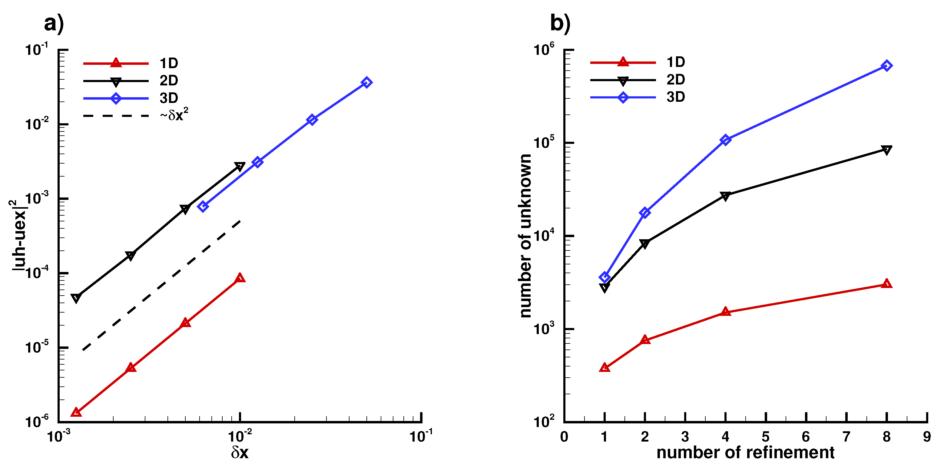
Appendix B.1. Laplace Equation Convergence Rate

We consider the Laplace equation:
Δ u = f ( x ) i n Ω , u = g ( x ) o n Ω ,
where Ω { R 1 , R 2 , R 3 } , x = x in R 1 , x = ( x , y ) in R 2 and x = ( x , y , z ) in R 3 .
Following the example in oomph-lib’s(https://oomph-lib.github.io/oomph-lib/doc/poisson/eighth_sphere_poisson/html/, accessed on 27 August 2023), we take the following exact solution in R 3 :
u e x ( x ) = tanh 1 α ( x x 0 ) · N | N | L 2 ,
where x = ( x , y , z ) is the vector of the spatial coordinates, and the vectors x 0 = x 0 , y 0 , z 0 and N = ( N 1 , N 2 , N 3 ) are constants. Noting that for large values of the constant α the solution varies rapidly across the plane through x 0 whose normal is given by N . The corresponding right hand side of (A5) using (A6) is given by:
f ( x ) = 2 α 2 tanh 2 1 α ( x x 0 ) · N | N | L 2 1 tanh 1 α ( x x 0 ) · N | N | L 2 , g ( x ) = u e x ( x ) .
In this section, we investigate the convergence rate of (A5) in Figure A6 and we show the result in Figure A7 of the 1D problem on a line segment [ R , R ] , in Figure A8 of the 2D problem on a circle C ( ( 0 , 0 ) , R ) , in Figure A9 of the 3D problem on a sphere S ( ( 0 , 0 , 0 ) , R ) and finally in Figure A6a) the different convergence rate of the 1D, 2D, and 3D problem of (A5) and in Figure A6b) the number of unknowns used for each case.
The following parameters were taken for the following tests:
R = 0.5 , α = 50 , N = ( 1 ) , x 0 = ( 0 ) , Δ x = 1 . e 2 / nref in 1 D , R = 0.5 , α = 50 , N = ( 1 , 1 ) , x 0 = ( 0 , 0 ) , Δ x = 1 . e 2 / nref in 2 D , R = 0.5 , α = 50 , N = ( 1 , 1 , 1 ) , x 0 = ( 0 , 0 , 0 ) , Δ x = 5 . e 2 / nref in 3 D ,
where nref is the number of refinement nref = { 1 , 2 , 4 , 8 } .
An important tool in FreeFem++ is mesh adaptation. It allows us to reduce the computational time, while keeping a high degree of accuracy. The mesh is adapted in 1D by taking more points between [-R/2,R/2] ( Δ x = 1 . e 2 / n r e f ) and Δ x = 1 . e 1 / n r e f in [-R,-R/2]∪[R/2,R]. In 2D, we use the adaptmesh command of FreeFem++ which creates a new mesh adapted to the Hessian of the solution. In 3D, the adaptation is performed through the libraries mshmet and mmg ([43]), which are directly linked to FreeFem++.
We adapt the initial mesh around the exact solution using the following parameter:
hmax = R , errg = 1 . e 2 , ratio = 1.3 , iso = 1 , nbvx = 1 e 8 in 2 D , hgrad = 1.7 , aniso = 1 , normalization = 1 , nbregul = 1 , nosurf = 0 , mem = 4000 i n 3 D ,
and err = 1 . e 4 , hmin = Δ x are common parameters for the 2D and 3D case.
Figure A6. (a): Second-order accuracy with L 2 norm is obtained for the 3 cases using P 1 finite element, (b) number of unknowns of each case of refinement.
Symmetry 16 00189 g0a6
Figure A7. Numerical solution in the 1D case for different refinements, (a) nref = 1, (b) nref = 2, (c) nref = 4, (d) nref = 8.
Symmetry 16 00189 g0a7
Figure A8. Numerical solution in the 2D case for different refinements, (a) nref = 1, (b) nref = 2, (c) nref = 4, (d) nref = 8.
Symmetry 16 00189 g0a8aSymmetry 16 00189 g0a8b
Figure A9. Numerical solution in the 3D case (cut of x < 0 ) for different refinements, (a) nref = 1, (b) nref = 2, (c) nref = 4, (d) nref = 8.
Symmetry 16 00189 g0a9

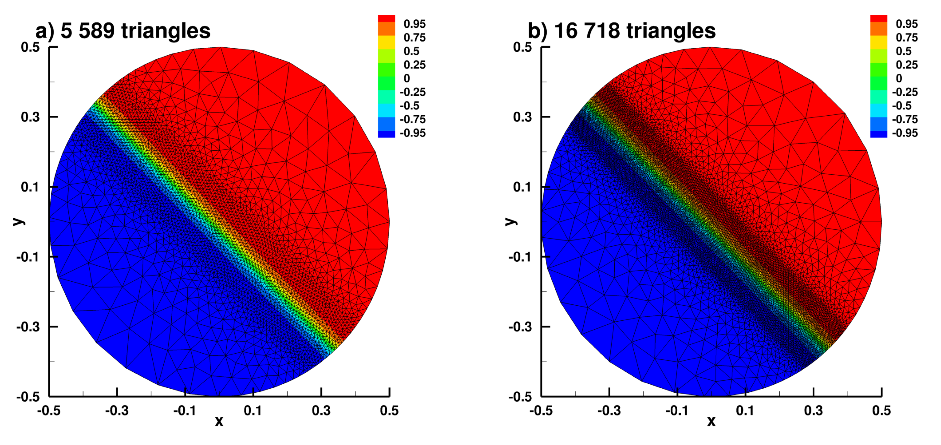
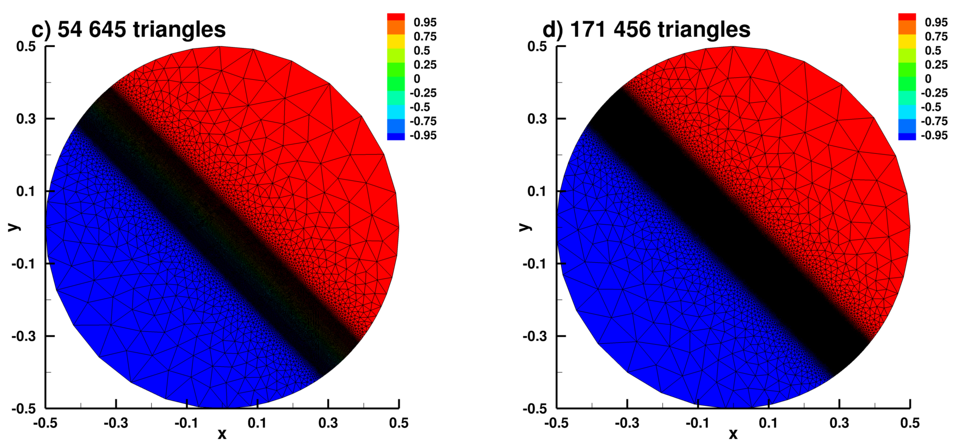
Appendix B.2. Laplace Equation Convergence Rate with Dirac Right Hand Side

We consider the Laplace equation:
Δ u = δ ( x x 0 ) in Ω , u = g ( x ) on Ω ,
where δ is the Dirac function. One of the solution for the (A10) in 3-dimensions is given by
u e x ( x ) = r ( x , x 0 ) if x > x 0 0 if x < = x 0 in 1 D , u e x ( x ) = 1 2 π ln r ( x , x 0 ) in 2 D , u e x ( x ) = 1 4 π r ( x , x 0 ) in 3 D ,
where r ( x , x 0 ) = | x x 0 | is the distance between x and x 0 .
For the convergence test, we consider that g ( x ) = u e x ( x ) . In Figure A10, we only show the convergence rate of (A10) in 2D and 3D, because in 1D we compare two affine functions. We show the result in Figure A11 of the 1D problem on a line segment [ R , R ] , in Figure A12 of the 2D problem on a circle C ( ( 0 , 0 ) , R ) , in Figure A13 of the 3D problem on a sphere S ( ( 0 , 0 , 0 ) , R ) , and finally in Figure A10a) the different convergence rates of the 2D and 3D problem of (A10), and in Figure A10b) the number of unknowns used for each case.
The following parameters were taken for the following tests:
R = 0.5 , x 0 = ( 0 ) , Δ x = 1 . e 2 / nref in 1 D , R = 0.5 , x 0 = ( 0 , 0 ) , Δ x = 1 . e 2 , split = nref in 2 D , R = . 5 , x 0 = ( 0 , 0 , 0 ) , Δ x = 5 . e 2 / nref in 3 D ,
where nref is the number of refinements nref= { 1 , 2 , 4 , 8 } and split defined in FreeFem++ to split the triangle using the nref part. We note that, since the used exact Equation (A11) is not defined in 2D and in 3D at x = x 0 , we were obliged to trunc around this point in 2D using r 2 > ( R / 40 ) 2 and in 3D using r 2 > ( R / 8 ) 2 , in order to compute the error between the exact solution and the numerical solution. On another hand, since the right hand side of the equation (A10) has a singularity, the classical results for regular right hand sides are not valid and a lower convergence rate can be expected, see [44,45].
Figure A10. (a): First-order accuracy with H 1 norm is obtained for the 2D and 3D cases using P 1 finite element, (b) number of unknowns of each case of refinement.
Symmetry 16 00189 g0a10
Figure A11. Numerical solution in 1D case for nref = 1.
Symmetry 16 00189 g0a11
Figure A12. Numerical solution in 2D case for nref = 4, (a) truncated solution on r 2 > ( R / 40 ) 2 , (b) full solution.
Symmetry 16 00189 g0a12
Figure A13. Numerical solution in 3D case (cut of x < 0 ) for nref = 4, (a) truncated solution on r 2 > ( R / 8 ) 2 , (b) full solution.
Symmetry 16 00189 g0a13

Appendix B.3. Laplace Equation with Dirac Right Hand Side

We consider the following Laplace equation with a Neumann boundary condition:
Δ u = a i δ ( x x i ) in Ω , u n = 0 on Ω ,
where a i is the amplitude of the Dirac function δ at x = x i and i = 1 3 a i δ ( x x i ) = 0 . In this section, we choose the position of the 3 Diracs x 1 = ( 0 , 0 , 0 ) , x 2 = ( 0 , R / 2 , 0 ) and x 3 = ( 0 , R / 2 , 0 ) and in Figure A14 we show the result of the 1D problem on a line segment [ R , R ] , in Figure A15 and Figure A16 of the 2D problem on a circle C ( ( 0 , 0 ) , R ) and in Figure A17 and Figure A18 of the 3D problem on a sphere S ( ( 0 , 0 , 0 ) , R ) .
Figure A14. Numerical solution in the 1D case.
Symmetry 16 00189 g0a14
Figure A15. Numerical solution in the 2D case, (a) full solution, (b) truncated solution on the axis x = 0.
Symmetry 16 00189 g0a15
Figure A16. The mesh is adapted around the position of the Diracs.
Symmetry 16 00189 g0a16
Figure A17. Numerical solution in the 3D case, (a) full isosurface solution, (b) truncated solution on the axis x = 0 and z = 0.
Symmetry 16 00189 g0a17
Figure A18. (a) The solution on the boundary of the domain, (b) the mesh is adapted around the position of the Diracs (cut of x < 0 ).
Symmetry 16 00189 g0a18
Figure A19. (A) Electrode configuration used for EEG recordings. Purple circles represent 30 active scalp contacts + 2 EOG contacts. (B) Preprocessing pipeline.
Symmetry 16 00189 g0a19

Appendix C. Data Preprocessing

All recordings were conducted using the Starstim-32 system by Neuroelectrics®. Particular attention was given to preventing acoustic and electromagnetic noise during EEG acquisition. Continuous EEG recordings were acquired through 30 NG Geltrode contacts placed on the scalp at a sampling frequency of 500 Hz (Figure A19A). Two additional electro-oculography electrodes (EOG) were placed above and below the right eye to capture eye-related artifacts. The reference electrodes (CMS and DRL) were affixed to the right ear lobe. The experimental protocol was designed using NIC2 software (Neuroelectrics, Barcelona, Spain), PsychoToolbox [46], and custom Matlab interfaces (Matlab 2021, the Mathworks, Natick, CA, USA).
Offline signal processing and analyses were carried out using the EEGLAB open-source toolbox [47] and custom Matlab scripts. Raw and continuous EEG signals underwent preprocessing through the pipeline outlined in Figure A19B (EEGLAB functions). The significance of independent component analysis (ICA) components was evaluated, and any identified as problematic were removed. Movement and muscle artifacts were visually identified and eliminated when necessary. The lowest cut-off frequency of the bandpass filters was set at 2 Hz, to eliminate the slow drifts present in several datasets.
The various trials (n = 100 + retest) were isolated from the continuous data, spanning from 1.5 s before image presentation to 4s after image presentation, resulting in 5.5-second-long epochs. It is noteworthy that, while most items could be named within this default response window, a few trials required more time. These specific trials were analyzed separately, and the actual number of regular epochs is detailed in the subsequent analyses.

References

  1. Adrian, E.D.; Yamagiwa, K. The origin of the Berger rhythm. Brain 1935, 58, 323–351. [Google Scholar] [CrossRef]
  2. Muller, L.; Chavane, F.; Reynolds, J.; Sejnowsk, T.J. Cortical travelling waves: Mechanisms and computational principles. Nat. Rev. Neurosci. 2018, 19, 255–268. [Google Scholar] [CrossRef] [PubMed]
  3. Meyer-Baese, L.; Watters, H.; Keilholz, S. Spatiotemporal patterns of spontaneous brain activity: A mini-review. Neurophotonics 2022, 9, 032209. [Google Scholar] [CrossRef]
  4. Klimesch, W.; Hanslmayr, S.; Sauseng, P.; Gruber, W.R.; Doppelmayr, M. P1 and Traveling Alpha Waves: Evidence for Evoked Oscillations. J. Neurophysiol. 2007, 97, 1311–1318. [Google Scholar] [CrossRef] [PubMed]
  5. Patten, T.M.; Rennie, C.J.; Robinson, P.A.; Gong, P. Human Cortical Traveling Waves: Dynamical Properties and Correlations with Responses. PLoS ONE 2012, 7, e38392. [Google Scholar] [CrossRef] [PubMed]
  6. Massimini, M.; Huber, R.; Ferrarelli, F.; Hill, S.; Tononi, G. The Sleep Slow Oscillation as a Traveling Wave. J. Neurosci. 2004, 24, 6862–6870. [Google Scholar] [CrossRef] [PubMed]
  7. Alamia, A.; VanRullen, R. Alpha oscillations and traveling waves: Signatures of predictive coding? PLoS Biol. 2019, 17, e3000487. [Google Scholar] [CrossRef] [PubMed]
  8. Sato, T.K.; Nauhaus, I.; Carandini, M. Traveling Waves in Visual Cortex Neuron 2012, 75, 218–229. 75.
  9. Zauner, A.; Gruber, W.; Himmelstoß, N.A.; Lechinger, J.; Klimesch, W. Lexical access and evoked traveling alpha waves. NeuroImage 2014, 91, 252–261. [Google Scholar] [CrossRef] [PubMed]
  10. Benitez-Burraco, A.; Murphy, E. Why Brain Oscillations Are Improving Our Understanding of Language. Front. Behav. Neurosci. 2019, 13, 190. [Google Scholar] [CrossRef]
  11. Alexander, D.M.; Jurica, P.; Trengove, C.; Nikolaev, A.R.; Gepshtein, S.; Zvyagintsev, M.; Mathiak, K.; Schulze-Bonhage, A.; Ruscher, J.; Ball, T.; et al. Traveling waves and trial averaging: The nature of single-trial and averaged brain responses in large-scale cortical signals. NeuroImage 2013, 73, 95–112. [Google Scholar] [CrossRef]
  12. Nir, Y.; Staba, R.J.; Andrillon, T.; Vyazovskiy, V.V.; Cirelli, C.; Fried, I.; Tononi, G. Regional Slow Waves and Spindles in Human Sleep. Neuron 2011, 70, 153–169. [Google Scholar] [CrossRef]
  13. Muller, L.; Piantoni, G.; Koller, D.; Cash, S.S.; Halgren, E.; Sejnowski, T.J. Rotating waves during human sleep spindles organize global patterns of activity that repeat precisely through the night. eLife 2016, 5, e17267. [Google Scholar] [CrossRef]
  14. Huang, X.; Xu, W.; Liang, J.; Takagaki, K.; Gao, X.; Wu, J. Spiral Wave Dynamics in Neocortex. Neuron 2010, 68, 978–990. [Google Scholar] [CrossRef]
  15. Lehmann, D.; Ozaki, H.; Pal, I. EEG alpha map series: Brain micro-states by space-oriented adaptive segmentation. Electroencephalogr. Clin. Neurophysiol. 1987, 67, 271–288. [Google Scholar] [CrossRef]
  16. Koenig, T.; Lehmann, D.; Merlo, M.C.G.; Kochi, K.; Hell, D.; Koukkou, M. A deviant EEG brain microstate in acute, neuroleptic-naive schizophrenics at rest. Eur. Arch. Psychiatry Clin. Neurosci. 1999, 249, 205–211. [Google Scholar] [CrossRef] [PubMed]
  17. De Menendez, R.G.; Murray, M.M.; Michel, C.M.; Martuzzi, R.; Andino, S.L.G. Electrical neuroimaging based on biophysical constraints. NeuroImage 2004, 21, 527–539. [Google Scholar] [CrossRef] [PubMed]
  18. Yuan, H.; Zotev, V.; Phillips, R.; Drevets, W.C.; Bodurka, J. Spatiotemporal dynamics of the brain at rest—Exploring EEG microstates as electrophysiological signatures of BOLD resting state networks. NeuroImage 2012, 60, 2062–2072. [Google Scholar] [CrossRef] [PubMed]
  19. Brechet, L.; Brunet, D.; Birot, G.; Gruetter, R.; Michel, C.M.; Jorge, J. Capturing the spatiotemporal dynamics of self-generated, task-initiated thoughts with EEG and fMRI. NeuroImage 2019, 194, 82–92. [Google Scholar] [CrossRef] [PubMed]
  20. Hassan, M.; Benquet, P.; Biraben, A.; Berrou, C.; Dufor, O.; Wendling, F. Dynamic reorganization of functional brain networks during picture naming. Cortex 2015, 73, 276–288. [Google Scholar] [CrossRef] [PubMed]
  21. Grappe, A.; Sarma, S.V.; Sacre, P.; Gonzalez-Martınez, J.; Liegeois-Chauvel, C.; Alario, F.-X. An intracerebral exploration of functional connectivity during word production. J. Comput. Neurosci. 2018, 46, 125–140. [Google Scholar] [CrossRef] [PubMed]
  22. Hartwigsen, G.; Stockert, A.; Charpentier, L.; Wawrzyniak, M.; Klingbeil, J.; Wrede, K.; Obrig, H.; Saur, D. Short-term modulation of the lesioned language network. eLife 2020, 9, e54277. [Google Scholar] [CrossRef]
  23. Laganaro, M.; Python, G.; Toepel, U. Dynamics of phonological–phonetic encoding in word production: Evidence from diverging ERPs between stroke patients and controls. Brain Lang. 2013, 126, 123–132. [Google Scholar] [CrossRef]
  24. Mheich, A.; Dufor, O.; Yassine, S.; Kabbara, A.; Biraben, A.; Wendling, F.; Hassan, M. HD-EEG for tracking sub-second brain dynamics during cognitive tasks. Sci. Data 2021, 8, 32. [Google Scholar] [CrossRef]
  25. Hooi, L.S.; Nisar, H.; Voon, Y.V. Tracking of EEG Activity using Topographic Maps. In Proceedings of the 2015 IEEE International Conference on Signal and Image Processing Applications (ICSIPA), Kuala Lumpur, Malaysia, 19–21 October 2015. [Google Scholar]
  26. Wackermann, J.; Lehmann, D.; Michel, C.M.; Strik, W.K. Adaptive segmentation of spontaneous EEG map series into spatially defined microstates. Int. J. Psychophysiol. 1993, 14, 269–283. [Google Scholar] [CrossRef]
  27. Buzsaki, G.; Anastassiou, C.A.; Koch, C. The origin of extracellular fields and currents—EEG, ECoG, LFP and spikes. Nat. Rev. Neurosci. 2016, 13, 407–420. [Google Scholar] [CrossRef]
  28. Jatoi, M.A.; Kamel, N. Brain Source Localization Using EEG Signal Analysis; Taylor & Francis Group: Boca Raton, FL, USA, 2018. [Google Scholar]
  29. Saturnino, G.B.; Siebner, H.R.; Thielscher, A.; Madsen, K.H. Accessibility of cortical regions to focal tes: Dependence on spatial position, safety, and practical constraints. NeuroImage 2019, 203, 116183. [Google Scholar] [CrossRef] [PubMed]
  30. Saturnino, G.B.; Madsen, K.H.; Siebner, H.R.; Thielscher, A. How to target inter-regional phase synchronization with dual-site Transcranial Alternating Current Stimulation. NeuroImage 2017, 163, 68–80. [Google Scholar] [CrossRef] [PubMed]
  31. Saturnino, G.B.; Puonti, O.; Nielsen, J.D.; Antonenko, D.; Madsen, K.H.; Thielscher, A. Simnibs 2.1: A comprehensive pipeline for individualized electric field modelling for transcranial brain stimulation. In Brain and Human Body Modeling; Makarov, S., Horner, M., Noetscher, G., Eds.; Springer: Cham, Switzerland, 2019. [Google Scholar]
  32. Volpert, V.; Xu, B.; Tchechmedjiev, A.; Harispe, S.; Aksenov, A.; Mesnildrey, Q.; Beuter, A. Characterization of spatiotemporal dynamics in EEG data during picture naming with optical flow patterns. Math. Biosci. Eng. 2023, 20, 11429–11463. [Google Scholar] [CrossRef] [PubMed]
  33. Aksenov, A.; Renaud-D’Ambra, M.; Volpert, V.; Beuter, A. Phase-shifted tACS can modulate cortical alpha waves in human subjects. Cogn. Neurodynamics 2023, in press. [Google Scholar] [CrossRef]
  34. Lehmann, D.; Skrandies, W. Reference-free identification of components of checkerboardevoked multichannel potential fields. Electroencephalogr. Clin. Neurophysiol. 1980, 48, 609–621. [Google Scholar] [CrossRef]
  35. Lehmann, D.; Skrandies, W. Spatial Analysis of Evoked Potentials in Man—A review. Prog. Neurobiol. 1984, 23, 227–250. [Google Scholar] [CrossRef]
  36. Murray, M.M.; Brunet, D.; Michel, C.M. Topographic ERP analyses: A step-by-step tutorial review. Brain Topogr. 2008, 20, 249–264. [Google Scholar] [CrossRef] [PubMed]
  37. Chantsoulis, M.; Polrola, P.; Goral-Polrola, J.; Hajdukiewicz, A.; Supinski, J.; Kropotov, J.D.; Pachalska, M. Application of ERPs neuromarkers for assessment and treatment of a patient with chronic crossed aphasia after severe TBI and long-term coma—Case report. Ann. Agric. Environ. Med. 2017, 24, 141–147. [Google Scholar] [CrossRef] [PubMed]
  38. Laganaro, M. Inter-study and inter-Individual Consistency and Variability of EEG/ERP Microstate Sequences in Referential Word Production. Brain Topogr. 2017, 30, 785–796. [Google Scholar] [CrossRef] [PubMed]
  39. Ermentrout, G.B.; Kleinfeld, D. Traveling Electrical Waves in Cortex: Insights from Phase Dynamics and Speculation on a Computational Role the results. Neuron 2001, 29, 33–44. [Google Scholar] [CrossRef] [PubMed]
  40. Zhang, H.; Watrous, A.; Patel, A.; Jacobs, J. Theta and Alpha Oscillations Are Traveling Waves in the Human Neocortex. Neuron 2018, 98, 1269–1281. [Google Scholar] [CrossRef] [PubMed]
  41. Mheich, A.; Hassan, M.; Khalil, M.; Berrou, C.; Wendling, F. A new algorithm for spatiotemporal analysis of brain functional connectivity. J. Neurosci. Methods 2015, 242, 77–81. [Google Scholar] [CrossRef] [PubMed]
  42. Hecht, F. New developments in Freefem++. Journal of Numerical Mathematics 2012, 20, 251–266. [Google Scholar] [CrossRef]
  43. Dapogny, C.; Dobrzynski, C.; Frey, P. Three-dimensional adaptive domain remeshing, implicit domain meshing, and applications to free and moving boundary problems. J. Comput. Phys. 2014, 262, 358–378. [Google Scholar] [CrossRef]
  44. Scott, R. Finite element convergence for singular data. J. Numer. Math. 1973, 21, 317–327. [Google Scholar] [CrossRef]
  45. Bradji, A.; Holzbecher, E. On the Convergence Order in Sobolev Norms of COMSOL Solutions; WIAS: Berlin, Germany, 2008. [Google Scholar]
  46. Brainard, D.H. The Psychophysics Toolbox; Brill: Leiden, The Netherlands, 1997. [Google Scholar] [CrossRef]
  47. Delorme, A.; Makeig, S. EEGLAB: An open source toolbox for analysis of single-trial EEG dynamics including independent component analysis. J. Neurosci. Methods 2004, 134, 9–21. [Google Scholar] [CrossRef] [PubMed]
Figure 1. Analytical approximation of a solution to Equation (1) with three point-wise sources. The curves show the values of the solution in time at different space points (see Appendix A for more details). (A) Sources with equal phases and frequencies, (B) different phases and equal frequencies, (C) different frequencies.
Symmetry 16 00189 g001
Figure 2. Two snapshots of the potential distribution on the upper surface of the sphere in numerical simulations of Equation (1). There are three sources with the same frequency and phases ( k i = 10 Hz, ϕ i = 0 ). The location of the sources approximately corresponds to the centers of the hot spots. For standing waves, oscillations of the potential occur without motion of the hot spots. The right panel shows the solution with inverse sign (time shift) compared to the left panel.
Symmetry 16 00189 g002
Figure 3. Snapshots of the potential distribution on the upper surface of the sphere in numerical simulations of Equation (1). There are three sources with different frequencies ( k 1 = 9 Hz, k 2 = 10 Hz, ϕ i = 0 ). Consecutive snapshots for the rotating regime show the motion of the hot spots between two neighboring sources.
Symmetry 16 00189 g003
Figure 4. Snapshots of the potential distribution on the upper surface of the sphere in numerical simulations of Equation (1). There are four sources with different frequencies (lower source k 1 = 9 Hz, left and right sources k 2 = 10 Hz, ϕ i = 0 , upper source is return source, see (4)). Consecutive snapshots show one period of the symmetric regime. The hot spot at the bottom (upper left panel) splits into two spots, which move up to the left and right sources (upper right panel). From there, they move to the upper source and merge (bottom left). Finally, the hot spot from the top descends along the symmetry line towards the lower source (bottom right). The color map corresponds to the value of solution at the cutting plane containing the sources (shown as dots).
Symmetry 16 00189 g004
Figure 5. Numerical modeling of tACS (two stimulation electrodes and one return electrode) with the software SimNIBS. Each curve corresponds to the electric potential at one of the 27 electrodes. Three cases are studied: (1) the case of equal frequencies (10 Hz) and phases (left) corresponds to standing waves, (2) the case of equal frequencies and different phases (middle) describes out-of-phase oscillations, (3) different frequencies (10 Hz and 11 Hz, right) produce modulated oscillations. The last two cases correspond to the rotating regime (see Figure 6). Bold black lines indicate time-dependent GFP. Reprinted from [32].
Symmetry 16 00189 g005
Figure 6. (A) One period of a rotating regime in the data simulated using the software SimNIBS. There are three sources with different frequencies (10 and 11 Hz). The hot spot moves counter clock-wise from the left source (upper left) to the lower source (upper right), and then to the upper source (lower middle). It is essential to note that the rotation is non-uniform; the advancement of the forward front is succeeded by the progression of the backward fronts. The yellow dots indicate the maximum potential within a specific time window corresponding to time t and certain preceding time points. The straight black lines represent the transitions of this maximum. Each map in the upper row is paired with a corresponding one directly below it, featuring a reversed sign (hot/cold color). (B) Schematic representation of the trajectory of the maximum of the solution. Reprinted from [32].
Symmetry 16 00189 g006
Figure 7. Upper panel: ERP signals (colored lines) for 30 electrodes averaged for 100 trials, and global field power (thick black line) for one subject in the theta range during the naming experiment. Time 0 corresponds to the image presentation, the large amplitude of the oscillations is consistent with image processing during the first 300 ms. Lower panel: scalp maps at the moments of time shown by the vertical lines in the upper panel. Synchronization of the electrodes and periodicity of the scalp maps correspond to a standing wave.
Symmetry 16 00189 g007
Figure 8. Upper panel: ERP signals (colored lines) for 30 electrodes averaged for 100 trials, and global field power (thick black line) for one subject in the alpha range during the naming experiment. Time 0 corresponds to the image presentation. Lower panel: scalp maps at the moments of time shown by the vertical lines in the upper panel. Asynchronization of the electrodes and the absence of exact periodicity of the scalp maps indicate a phase shift in the sources. Note that the amplitude of oscillations is close to constant.
Symmetry 16 00189 g008
Figure 9. Upper panel: ERP signals (colored lines) for 30 electrodes averaged for 100 trials for one subject in the beta range during the naming experiment. Time 0 corresponds to the image presentation. Lower panel: scalp maps at the moments of time shown by the vertical lines in the upper panel. Modulated oscillations of the electrodes indicate different frequencies of the sources. Note that the brain maps are close to periodic.
Symmetry 16 00189 g009
Figure 10. Spatiotemporal dynamics in the individual trial of the EEG data in the alpha range for one subject. The moments of time are indicated in the images. Negative time corresponds to the next image preparation, but similar behavior was also observed during other stages of image processing and speech production. Consecutive snapshots correspond to one period of rotating regime. Note that the rotation is not uniform, propagation of forward and backward fronts alternate with each other. Images in the upper and lower rows are pairwise similar to each other with opposite colors. Direction of rotation changes after several periods. This regime is similar to the rotating regime observed in the numerical simulations (Figure 3 and Figure 6).
Symmetry 16 00189 g010
Figure 11. Spatiotemporal dynamics in the individual trial of the EEG data for the same subject and trial as in Figure 10 but during a different time interval after the image presentation. Consecutive snapshots correspond to one period of the symmetric regime. The hot spot at the bottom splits into two spots moving upwards along the borders. They merge at the top and descend along the symmetry line. Images in the upper and lower rows are pairwise similar to each other with opposite colors. Note that the largest value of the potential (dark red) changes between left and right hot spots. Several (4–5) periods of this regime follow each other. The symmetry axis can change during another time interval; that is, form a nonzero angle with the vertical direction. This regime is similar to the symmetric regime observed in the numerical simulations (Figure 4).
Symmetry 16 00189 g011
Figure 12. Unfolded trajectory showing the position of the potential maximum for some subject during one trial and frequency 22 Hz. Time 0 corresponds to image presentation, the red line (1200 ms) corresponds to the beginning of speech production. The whole trial can be split into the time intervals, where the trajectory periodically repeats its motion. These time intervals are shown by the color of the trajectory and by the straight lines in the rectangle below the trajectory (till time 1450 ms). The self-similarity of the trajectory was determined using the Hausdorff distance between the polygons formed by the trajectory. Note that the vertices of the trajectories are formed by 2–3 neighboring points, indicating local motion of the maximum. These vertices are separated by distant jumps (cf. Figure 6). There are usually three or four vertices that correspond to the rotating and to symmetric regimes. Longer sequences of neighboring points around 2000 ms correspond to moving waves (Section 3.5).
Symmetry 16 00189 g012
Figure 13. Brain maps for two different subject at the frequency 22 Hz, (A) subject with aphasia, (B) control subject (matched for gender and age). Each dot corresponds to the beginning or to the end of the moving waves registered during 10 trials in the repetition of the same word (‘chien’ in French, i.e., dog). The curves connecting the dots show the trajectories of the maximum, and their color indicates the final moment in time of the wave existence relative to the image presentation (cf. the color bar). The areas of dot accumulation determined by the density map analysis are indicated by the black circles. Note the difference between the two maps and larger white areas without waves for the subject with aphasia.
Symmetry 16 00189 g013
Disclaimer/Publisher’s Note: The statements, opinions and data contained in all publications are solely those of the individual author(s) and contributor(s) and not of MDPI and/or the editor(s). MDPI and/or the editor(s) disclaim responsibility for any injury to people or property resulting from any ideas, methods, instructions or products referred to in the content.

