Navigation Route Planning for Tourism Intelligent Connected Vehicle Based on the Symmetrical Spatial Clustering and Improved Fruit Fly Optimization Algorithm
Abstract
1. Introduction
1.1. Research Background and Problem Discussion
- (1)
- Relationship 1: The POIs on the ICV routes are the targets for tourists to visit. Whether the tourists can generate the maximum benefit motivation from visiting the POIs is an important evaluation indicator of whether the ICV routes are the optimal ones. Therefore, each POI on the optimal ICV route must be the one that the tourists are most interested in and willing to visit. By constructing the relationship between POI functional attributes and tourist interest attributes, we recommend POIs for tourists and establish the relationship between the ICV routes and the tourists’ interests and demands.
- (2)
- Relationship 2: From the perspective of energy conservation and travel cost control for the tourists, the ICVs will produce travel costs and fees in moving and ferrying tourists between different POIs, which will ultimately be paid by the tourists. From the perspective of saving travel costs, the ICV routes are directly related to tourist motivation benefits. The key to improving tourist satisfaction is to search for the ICV routes with the best POIs and the lowest travel cost. Thus, the modeling for the optimal ICV routes has close relationship to the tourists’ satisfaction.
1.2. Problem Solving Methods
2. Related Work and Analysis
2.1. Related Work and Limitation
2.2. The Difference and Advantage of Our Proposed Work
2.3. Our Proposed Method
- (1)
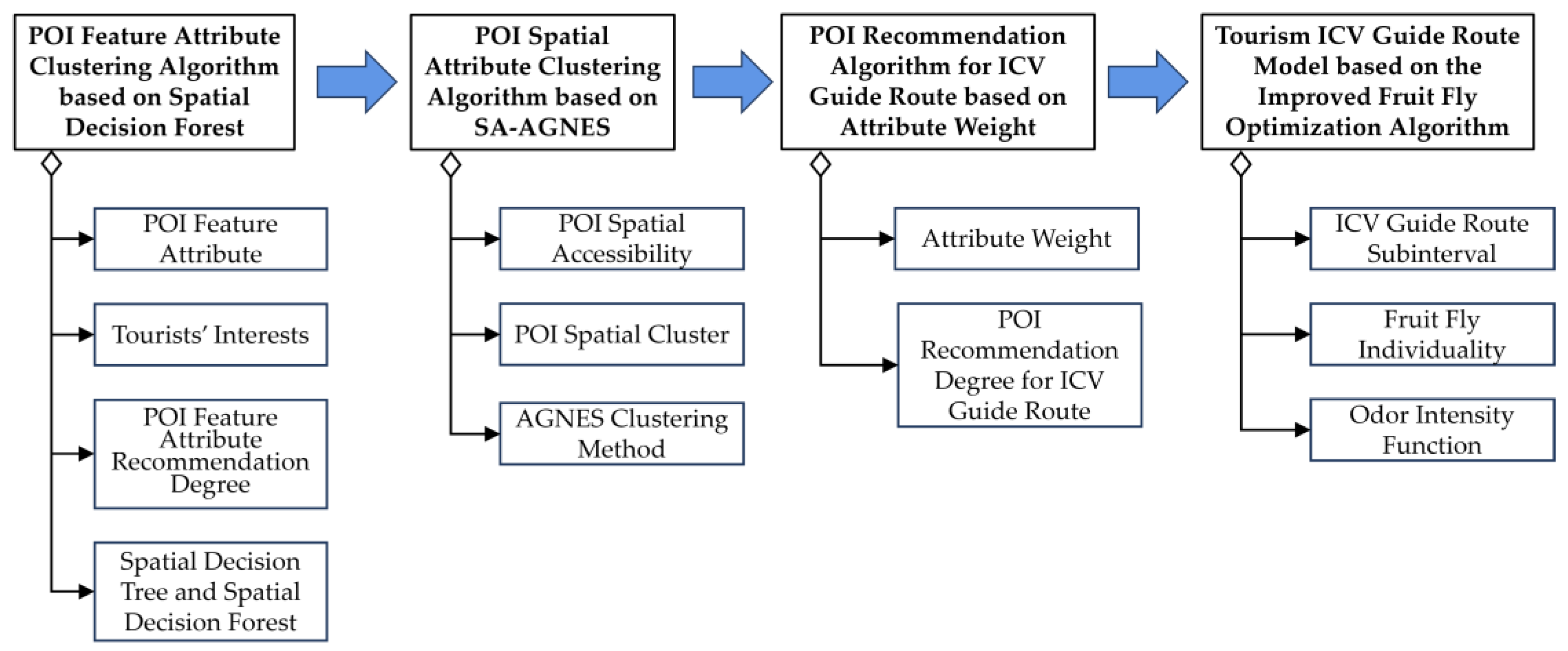
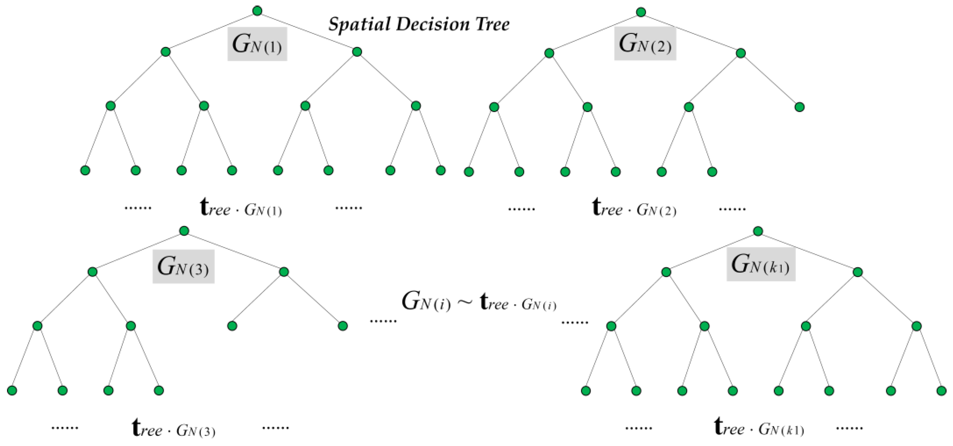
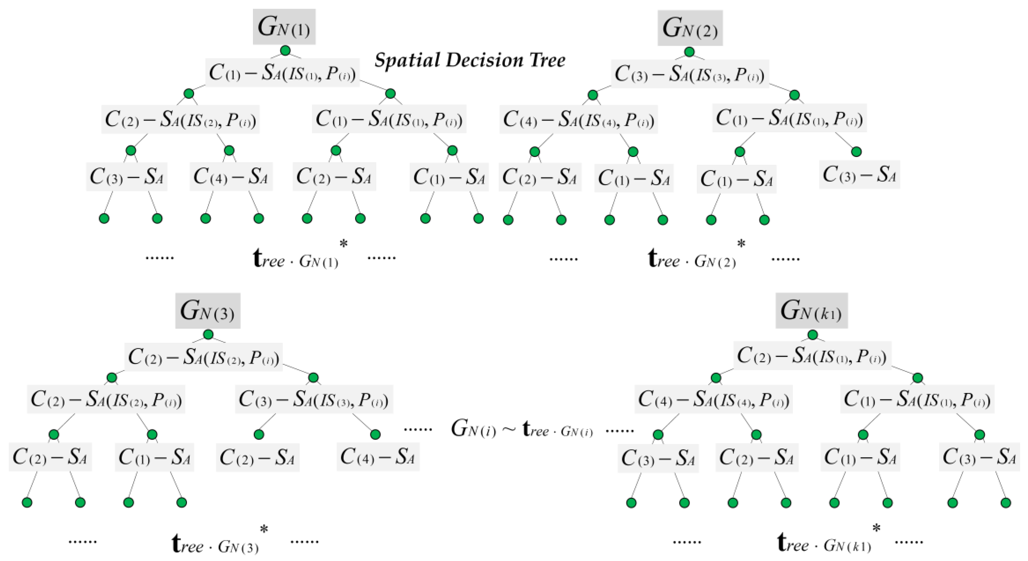
- We construct a POI feature attribute clustering algorithm based on the spatial decision forest, which clusters the urban POIs according to the root nodes with different natural attributes. The binary tree algorithm with the descending matching degree of tourists’ interests is proposed to generate a spatial decision tree. Each decision tree represents one feature attribute cluster. The construction of the spatial decision forest can output the POIs that best match tourists’ interests for ICVs.
- (2)
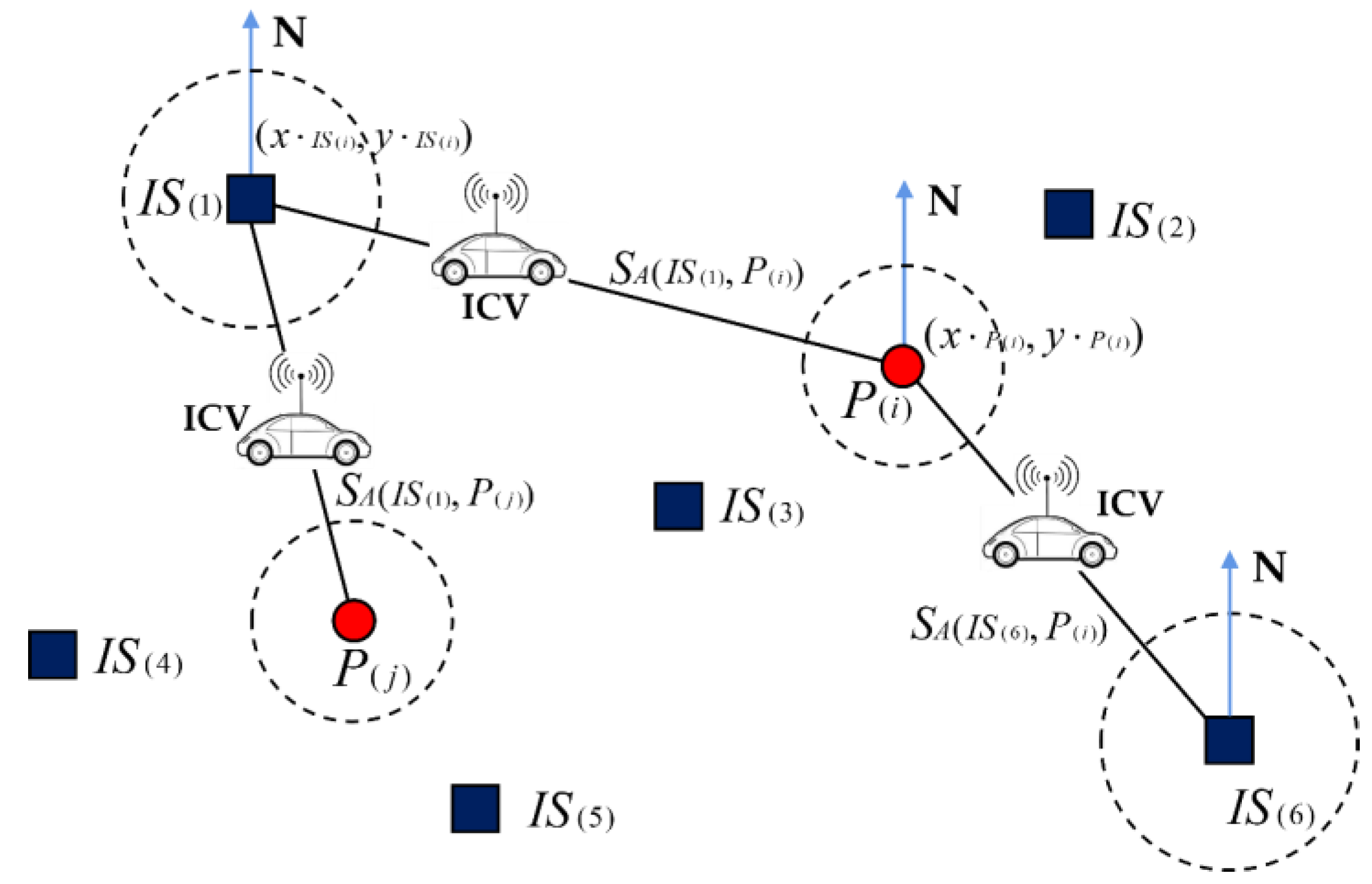
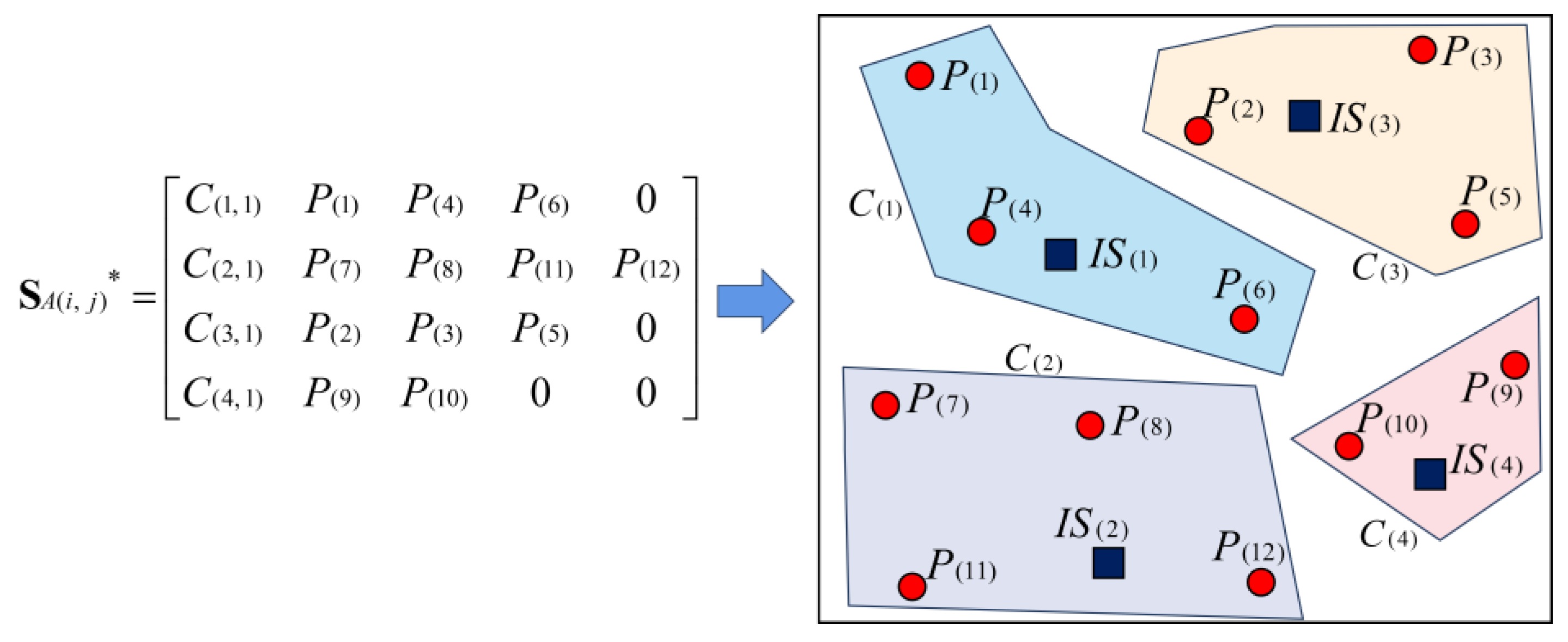
- We also construct a POI spatial attribute clustering algorithm based on the spatial accessibility and AGNES (SA-AGNES). Taking the ICV transfer stations as the core points of AGNES spatial clustering, the spatial attributes of POIs within the neighborhood of the transfer stations are determined by searching spatial accessibility, and the POIs are spatially clustered to determine the spatial relationship between the ICV transfer stations and neighboring POIs. Finally, the ICV intelligent decision-making system will output the POIs with the optimal spatial distributions.
- (3)
- We design and construct an optimal POI recommendation algorithm based on spatial clustering. In response to the control node selection problem of the tourism ICV navigation route-planning algorithm, we set the searching target as the POIs that best match tourists’ interests and have the optimal spatial distributions. The ICV intelligent decision-making system searches for POIs that tourists need to visit, and uses them as the precondition for the ICV route-planning algorithm.
- (4)
- Based on the modeling of the urban geospatial environment and traffic road conditions, we construct a tourism ICV navigation route model based on the improved fruit fly optimization algorithm. Using the ICV transfer stations and POIs as nodes, it outputs the tour route with the lowest travel cost under the geospatial constraints.
- (5)
- We design and perform the validation experiment and comparative experiment, which proves that the proposed algorithm can accurately output POIs that match tourists’ interests, and can find out the ICV navigation route with the lowest travel cost. Compared with the commonly used map route-planning methods and the traditional route-searching algorithms, the proposed algorithm can reduce the travel cost by 15.22% at most, and effectively reduce energy consumption of the ICV system, then finally improve the tourists’ satisfaction.
3. Methodology
3.1. The Optimal POI Recommendation Algorithm for Tourism ICV System
3.1.1. POI Feature Attribute Clustering Algorithm Based on Spatial Decision Forest
| Algorithm 1: The POI feature attribute clustering algorithm based on spatial decision forest |
| Input: POI natural attribute root nodes, POI feature attribute vector , POI feature attribute matrix , tourist interest measurement vector , tourist interest measurement matrix , disturbance factor Output: Spatial decision forest Step 1: As to attribute , take , construct spatial decision tree . Obtain POIs that meet , encode the POIs , , . Step 2: Calculate the , traverses , then output number of recommendation degrees . Step 3: Compare and , iterating :
Step 6: Turn back to Step 1. As to attribute , take . In line with the same algorithm from Step 2 to Step 5, construct the spatial decision tree . Step 7: As to attribute , traverse , output , , …, , relating to number of natural clusters . The number of decision tress consists of the spatial decision forest . The algorithm ends. |
3.1.2. POI Spatial Attribute Clustering Algorithm Based on SA-AGNES
| Algorithm 2: The POI spatial attribute clustering algorithm based on SA-AGNES |
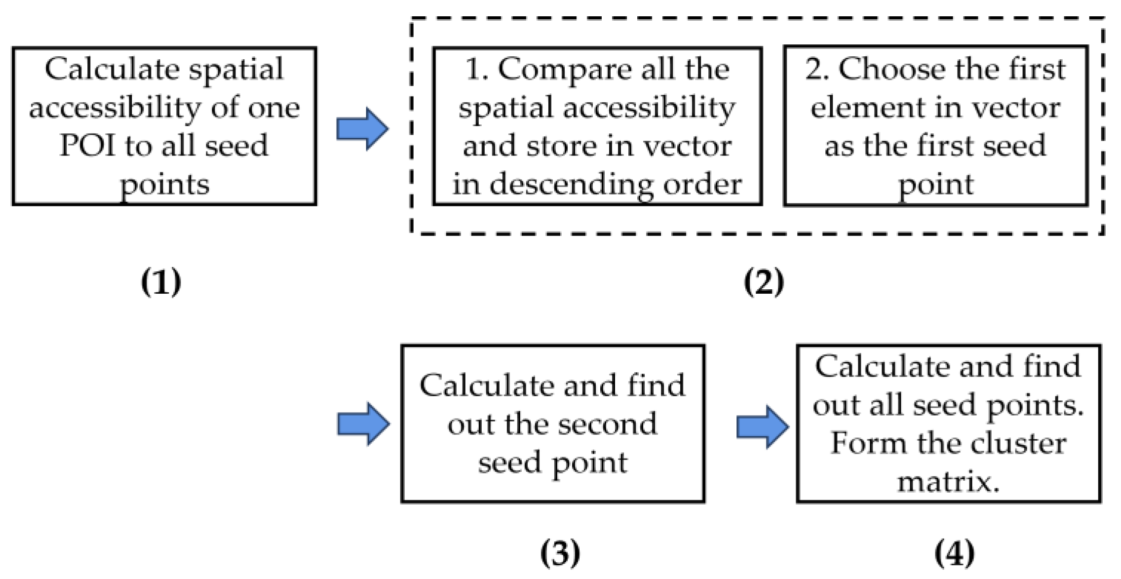
| Input: number of coordinates of ICV transfer stations , number of coordinates of POIs , the initialized seed points , and the initialized zero matrix for the dimension matrix . Initialize the dimension transition vector for spatial accessibility. Output: Full ranked matrix for cluster. Step 1: As to number of POIs , take , calculate the between and number of seed points . Step 2: Compare number of , in which traverses , . Step 2.1: Compare and , iterating :
Step 2.4: Loop iteration until , iteration ends. Output a full ranked vector . Take the seed point of the current element as the cluster seed point where the POI is located. Store into element of matrix , note . Step 3: For number of POIs , take and calculate the between and number of the seed points . According to the Step 2 algorithm, iterate and store in by descending order. At the end of the iteration , output a full ranked vector . Take the seed point of the current element as the cluster seed point where the POI is located. Store into element of matrix , note . Step 4: As to the number of POIs , iterating , and traversing . When a is iterated, store into element of matrix , note . Step 5: As to the , until the is iterated. Output the full ranked matrix , the algorithm ends. |
3.1.3. POI Recommendation Algorithm Based on Attribute Weight for ICV Navigation Route
- (1)
- The matching between the POI feature attributes and the tourists’ interests, i.e., feature attribute recommendation degree ;
- (2)
- When the ICV travels on the tour route, considering the urgent situations such as power outages, sudden malfunctions, traffic accidents, tourist suspensions and adverse weather conditions, the ICV tour route should surround the ICV transfer stations and search for the POIs with the best spatial accessibility within the cluster including .
- (3)
- The setting of attribute weight should balance and .
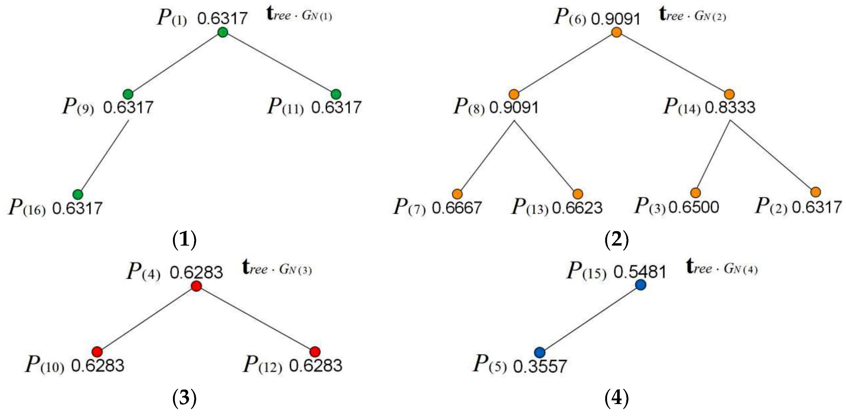
| Algorithm 3: The optimal POI recommendation algorithm based on the attribute weight for tourism ICVs |
| Input: Spatial topological forest , attribute weight factor Output: The best matched POIs for tourists’ interests. Step 1: Select decision tree of the decision forest . Calculate POI recommendation degrees for all nodes in the decision tree. Step 2: Construct the optimization algorithm for the maximum heap sorting decision tree . Step 2.1: Compare the root node with the child node in recommendation degree :
Step 2.4: Mark the cluster which the current recommendation degree of each node belongs to, and the optimization algorithm for the decision tree ends. Step 3: Select decision tree of the decision forest . Calculate POI recommendation degrees for all nodes in the decision tree. In line with the algorithm in Step 2, realize the optimization for . Traversing . Step 4: As to , until the is iterated. The optimization algorithm for the decision forest ends. Output the optimal POIs in each decision tree , relating clusters , and ICV transfer stations . |
3.2. Tourism ICV Navigation Route Model Based on the Improved Fruit Fly Optimization Algorithm
- (1)
- The searching for the route nodes has the feature of arbitrariness. When an ICV leaves a node to search for the next node, it has the feature of randomness in point selection, which is consistent with the characteristic of random searching by fruit flies;
- (2)
- The searching direction has the feature of arbitrariness. When an ICV leaves a node to search for the next node, it has directional randomness, which is consistent with the characteristic of random searching by fruit flies;
- (3)
- When an ICV selects a path node, randomly selecting the next node is equivalent to replacing a target node, which is related to changing a step size, and identical to the principle of the fruit fly optimization algorithm’s step-size searching.
- (4)
- The fruit fly optimization algorithm has the characteristic of population convergence. After each searching cycle, all the fruit flies fly towards the current optimal solution. During the searching process, individuals which are not the optimal solution can be excluded, and the convergence speed is fast.
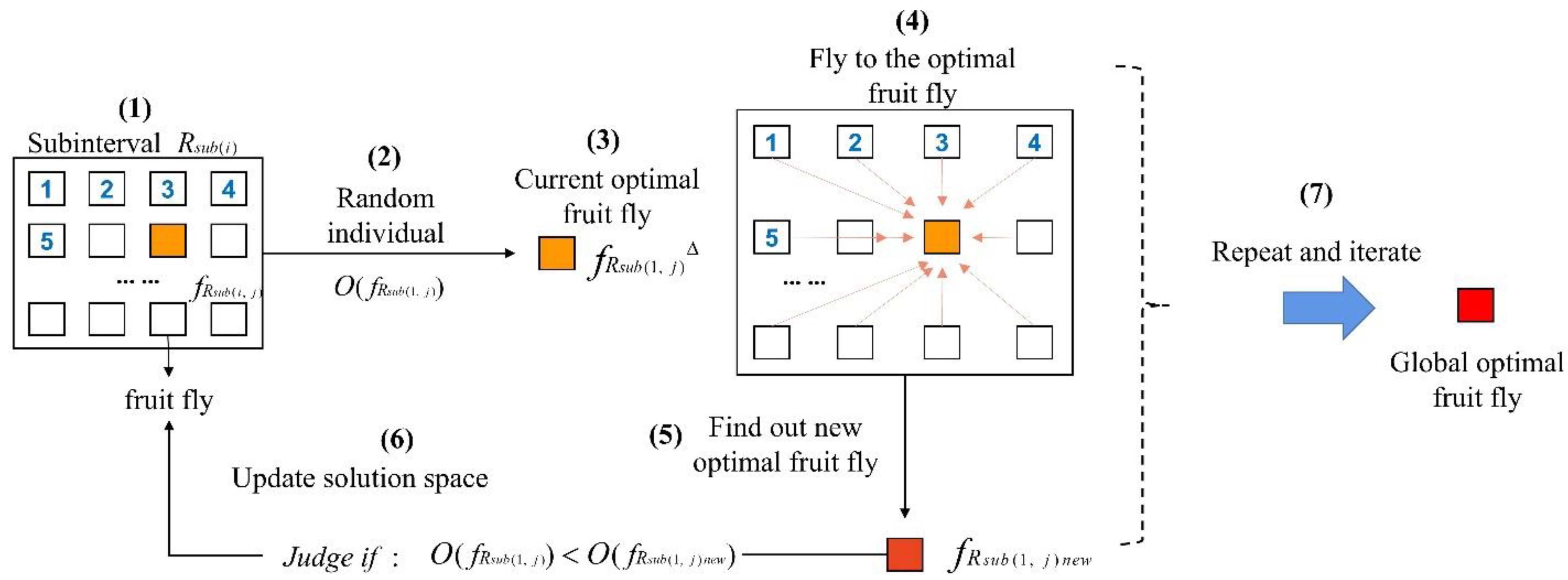
- (1)
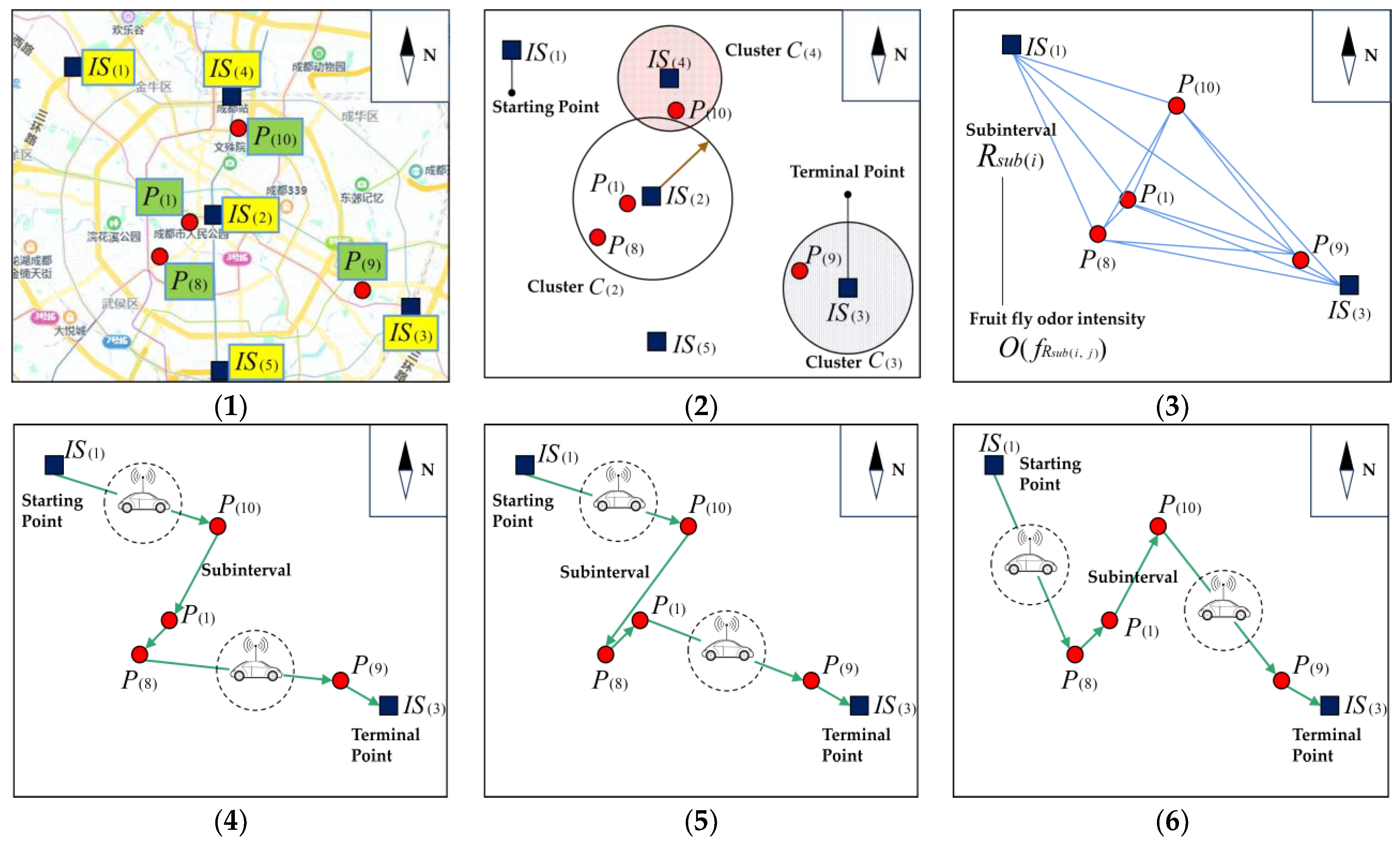
- Initialize the sub-interval , including number of nodes , starting point , and and terminal point , as shown in the Figure 9(1).
- (2)
- Step 1: Select or . Node is found, then a feasible path is formed, keep , as shown in the Figure 9(2).
- (3)
- Step 2: Select or . Node is found, then a feasible path is formed, keep , as shown in the Figure 9(3).
- (4)
- Step 3: Select , , or . Node is found, then a feasible path is formed, keep , as shown in the Figure 9(4).
- (5)
- Step 4: Select or . Node is found, then a feasible path is formed, keep , as shown in the Figure 9(5).
- (6)
- Step 5: Select or . Node is found, then a feasible path is formed, keep , as shown in the Figure 9(6).
- (7)
- Step 6: Node is found, then a feasible path is formed, keep , as shown in the Figure 9(7).
- (8)
- Step 7: Arrive at the POI and form a pathway , which constitutes one individual fruit fly , as shown in the Figure 9(8). The searching process ends.
| Algorithm 4: Tourism ICV navigation route model based on the improved fruit fly optimization algorithm |
| Input: Recommended POI, sub-interval , node for each sub-interval, starting point or , terminal point or . Output: Optimal ICV navigation route Step 1: As to the sub-interval , take , construct the optimal ICV route for the first sub-interval. Step 1.1: Initialize the fruit fly individual and solution space . Step 1.2: Set up the sub-interval model . Confirm the starting point , node , terminal point ; Step 1.3: Starting point of searches for node . Judge whether there exists a that will be absorbed into in :
Step 2: In line with the same algorithm as Step 1, as to the sub-interval , take , construct the optimal ICV route for the second sub-interval. Output solution space , including number of fruit fly individuals , namely . Step 3: Continue searching, and output solution space , including number of fruit fly individuals , namely . Traverse solution space , corresponding to . Output all fruit fly individuals for all sub-intervals in ICV navigation route. Step 4: Update locations in the fruit fly group . Iterate to calculate the optimal fruit fly individual for . Output the optimal navigation route for . Step 4.1: Randomly select a fruit fly individual as , calculate ; Step 4.2: As to , fly to by unit step size . Update locations in the fruit fly group . Set that after flying by unit step size, turns to , make judgement:
Step 5: Update locations in the fruit fly group , iterate to calculate the optimal fruit fly in , and output the optimal ICV navigation route in . Step 6: Update locations in the fruit fly group , iterate to calculate the optimal fruit fly in , and output the optimal ICV navigation route in , traversing . Output the optimal ICV navigation routes in all sub-intervals . Step 7: Connect all the optimal navigation routes in all from the starting point or to the terminal point or , and output the intact optimal ICV navigation route for tourists. |
4. Experiment and Result Analysis
4.1. Experimental Objectives
- (1)
- Goal 1: Test and verify the feasibility and accuracy of POI feature attribute recommendation results;
- (2)
- Goal 2: Test and verify the feasibility and accuracy of the spatial decision forest results;
- (3)
- Goal 3: Verify the feasibility and accuracy of the spatial topology forest results;
- (4)
- Goal 4: Verify the feasibility and accuracy of the recommendation decision forest and the recommended POI output results;
- (5)
- Goal 5: Verify the feasibility and accuracy of the recommended ICV tour route results;
- (6)
- Goal 6: Verify the advantages of the constructed ICV navigation route algorithm over traditional map route-planning methods and the commonly used shortest route-searching algorithms.
4.2. Experiment Process and Data Collection
4.2.1. Experiment Process and Metric Selection
- Experiment Process
- (1)
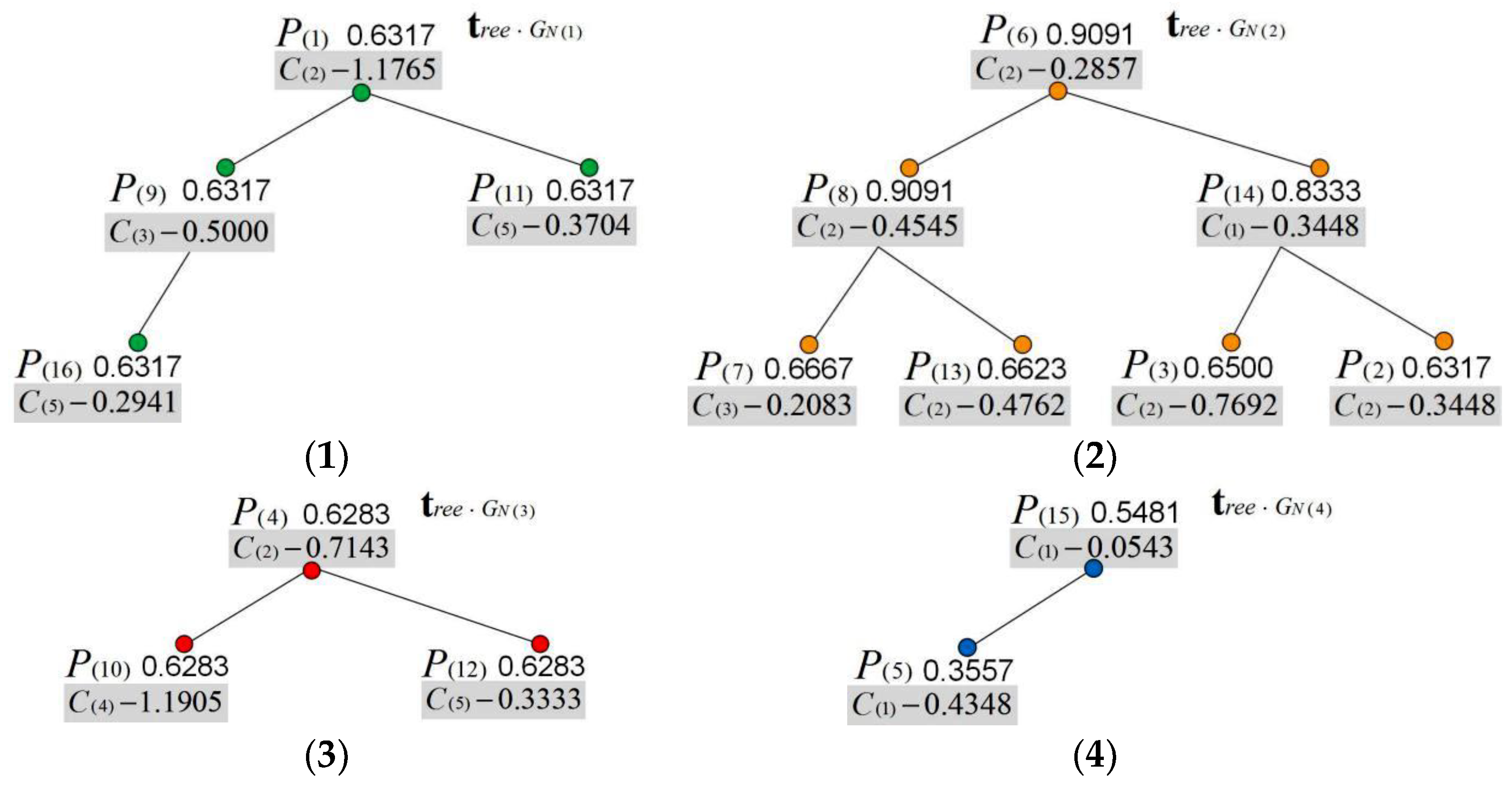
- Randomly select one tourist as the research subject, determine the natural attributes of all the POIs, including: “park and green land”, “cultural and historical commemoration”, “leisure shopping center”, and “amusement and theme park”. Determine the POI feature attribute vector and the POI feature attribute matrix , in which the POI feature attributes include : “travel cost”, : “travel time”, : “POI level (A-Class)”, and : “POI popularity”. Determine the tourist interest measurement vector and the tourist interest measurement matrix based on the POI feature attributes, then randomly determine and quantify the tourist interest vector, and calculate the POI feature attribute recommendation degree function , ultimately generating the spatial decision trees and the spatial decision forest .
- (2)
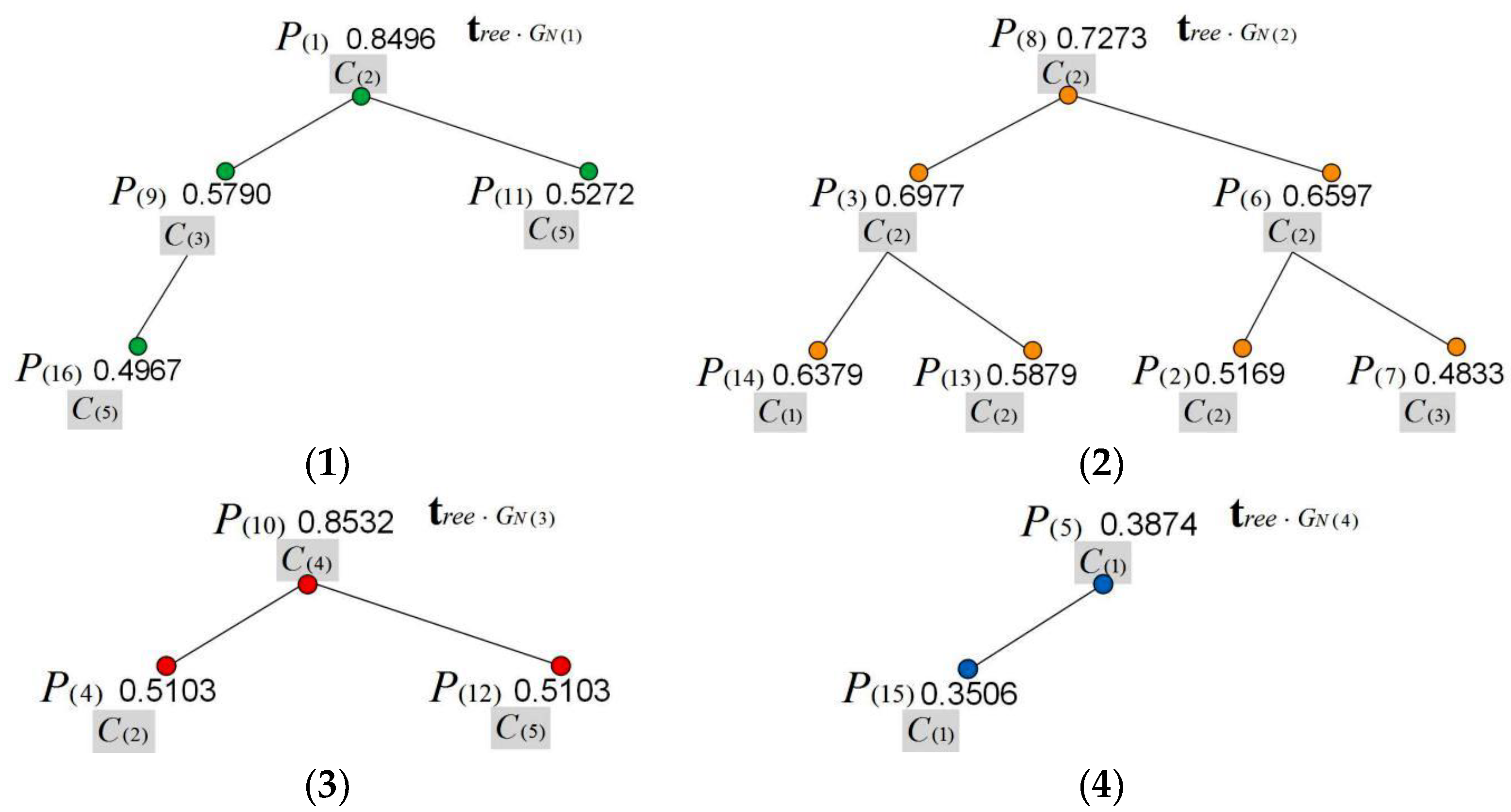
- Calculate the POI spatial accessibility using the spatial relationship between the ICV transfer station and the POI , generate the POI spatial clustering matrix , and determine the spatial clustering clusters with each ICV transfer station as the seed point. Generate the topological forest based on the spatial decision forest and the spatial clustering results.
- (3)
- Tourists determine the attribute weight factors . Calculate the POI recommendation degree based on the topological forest , and output the decision forest with the labeled spatial clusters and the recommendation degree . Determine the optimal POIs recommended to the tourist.
- (4)
- Use the constructed improved fruit fly optimization algorithm to output the optimal ICV navigation routes. Starting from the ICV transfer station selected by the tourist, the algorithm searches for the ICV navigation routes one by one through the recommended POIs, and outputs the route with the highest odor concentration function in each sub-interval . The terminal point of the ICV navigation route is the chosen ICV transfer station .
- (5)
- The route-searching methods embedded in the Gaode Map (GDM) and the Baidu Map (BDM), and the most representative route-searching algorithms Dijkstra and Floyd–Warshall, are set as the two control groups. Then we design the comparative experiment, in which the proposed algorithm is set as the experimental group, while the map route-planning methods and the commonly used route-searching algorithms are set as the two control groups. We compare the travel costs of our proposed algorithm with the control groups’ route-planning methods in outputting the optimal ICV navigation routes.
- 2.
- Metric Selection
- (1)
- Sub-interval weight difference
- (2)
- Route weight difference
- (3)
- Sub-interval mileage difference
- (4)
- Route mileage difference
- (5)
- Cost optimization ratio model
- (6)
- Algorithm time complexity
4.2.2. Data Collection
- (1)
- POIs within Chengdu city. POIs are classified according to their natural attributes and the results are shown in Table 1. The selection of POIs within the city meets the following conditions:
- (2)
- Representative ICV transfer stations. : Chadianzi Bus Station; : Tianfu Square; : Chengdu East Railway Station; : Chengdu Railway Station; : Chengdu South Railway Station. The five representative ICV transfer stations selected for the experiment are all the transportation hubs with the highest passenger flow, the longest operating hours, and located at the important control nodes in Chengdu city. They are distributed in the western, central, eastern, northern, and southern parts of Chengdu city, and are the most representative transportation hubs with the most significant geographical locations. Therefore, the five ICV transfer stations selected for the experiment can cover all the representative POIs, urban roads, and all the urban nodes within the experimental range, and their spatial locations are relatively average to all the POIs. The longitude and latitude coordinates of the ICV transfer stations have typical spatial attributes, which can be used to quickly calculate the spatial accessibility with POIs and generate the spatial clusters.
- (3)
- The feature attribute requirements for tourists that are input into the ICV decision-making system are shown in Table 2. Simultaneously, the feature attributes and spatial attributes of POIs are collected. Randomly select one tourist for the experiment and input his needs into the ICV decision-making system. To meet the matching algorithm between the tourist interests and POI feature attributes in POI recommendation, the demands that the tourist inputs into the ICV decision-making system should meet the following conditions:
- (4)
- Collect all road nodes between recommended POIs, and road nodes between POIs and ICV transfer stations. Collect road distances between adjacent road nodes. The process of collecting road nodes is as follows: ① Collect and determine all the ICV moving sub-intervals, and determine the starting and ending points of each sub-interval; ② Determine two control nodes for the ICV moving sub-interval, with each control node being an ICV transfer station or a POI; ③ Obtain all the connected roads between two control nodes in the city map, which can directly or indirectly connect the two control points; ④ Search for the road intersections from the starting control point to the ending control point. Encode each intersection when it is searched, and store it in the sub-interval node database; ⑤ Repeat the same searching for all sub-intervals; ⑥ Search for the distance between adjacent nodes in the city map and store it in the sub-interval node distance database.
4.3. Results and Analysis on POI Spatial Decision Forest and Topological Forest
4.3.1. Results on POI Feature Attribute Recommendation Degree and Spatial Decision Forest
4.3.2. Results on POI Spatial Topological Forest
4.3.3. Results Analysis on the POI Feature Attribute Recommendation Degree, Spatial Decision Forest and POI Spatial Topological Forest
4.4. Results and Analysis on Recommendation Degree, Recommendation Degree Decision Forest and Recommended POI
4.4.1. Results on Recommendation Degree, Recommendation Degree Decision Forest and Recommended POIs
4.4.2. Results Analysis on the Recommendation Degree, Recommendation Degree Decision Forest and Recommended POI
4.5. Results and Analysis on ICV Navigation Route
4.5.1. Results on ICV Navigation Route
4.5.2. Results Analysis on ICV Navigation Route
4.6. Results and Analysis on the Comparative Experiment
4.6.1. Method and Results of the Comparative Experiment
- (1)
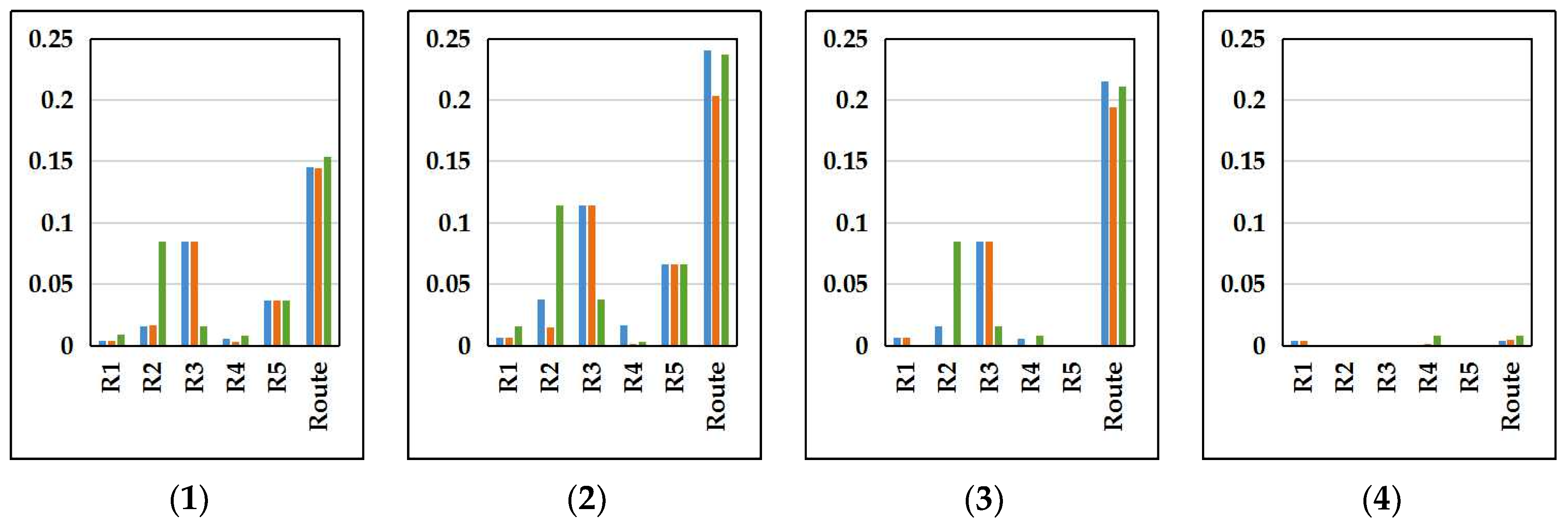
- The results shown in Table 8 are the comparison of the sub-interval weight and the route weight of the optimal ICV navigation route ICV-G1, and the suboptimal navigation routes ICV-G2 and ICV-G3 output by the three algorithms. The results shown in Table 9 are the comparison of the optimal and suboptimal ICV navigation routes in the sub-interval weight difference , route weight difference , and cost optimization ratio , between the control group and the experimental group. Figure 15 shows the comparison of the sub-interval weight difference , route weight difference , and cost optimization ratio , between the control group and the experimental group. Figure 15(1) represents the comparison between the GDA and the PRA. Figure 15(2) represents the comparison between the BDA and the PRA. Figure 15(3) represents the comparison between the DIJA and the PRA. Figure 15(4) represents the comparison between the FWA and the PRA. In each figure, the blue data columns represent the route P10,1,8,9, the brown data columns represent the route P10,8,1,9, and the green data columns represent the route P8,1,10,9.
- (2)
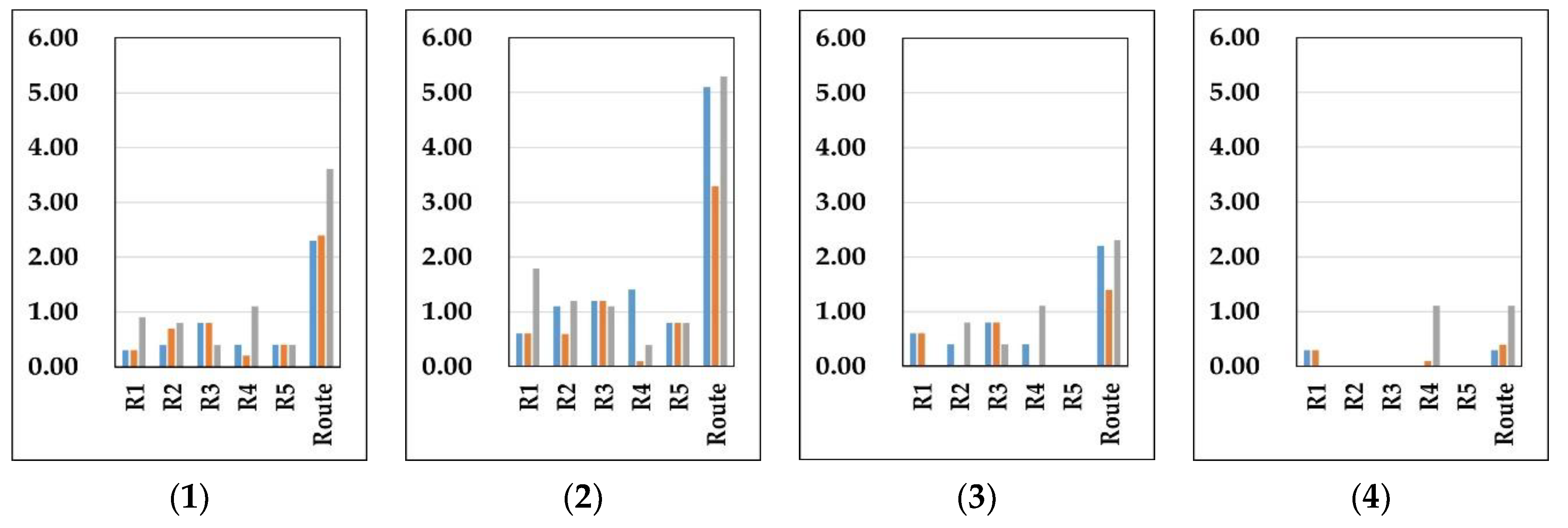
- The results shown in Table 10 are the comparison of sub-interval mileage and total route mileage of the optimal ICV guidance route ICV-G1, and the suboptimal guidance routes ICV-G2 and ICV-G3 output by each method of the control group and the experimental group. The results shown in the Table 11 are the comparisons of the sub-interval mileage difference , total route mileage difference , and cost optimization rate of the optimal and suboptimal ICV guidance routes output by each method, between the control group and the experimental group. Figure 16 shows the comparison of sub-interval mileage difference , route mileage difference , and cost optimization rate between the control group algorithms and the experimental group algorithm. Figure 16(1) represents the comparison between the GDA and the PRA. Figure 16(2) represents the comparison between the BDA and the PRA. Figure 16(3) represents the comparison between the DIJA and the PRA. Figure 16(4) represents the comparison between the FWA and the PRA. In each figure, the blue data columns represent the route P10,1,8,9, the brown data columns represent the route P10,8,1,9, and the green data column represents the route P8,1,10,9.
- (3)
- Table 12 shows the time complexity comparisons between the route-searching algorithm (PRA), the DIJA, and the FWA. According to the constraints of the urban geographic space and the tourism scenarios, the number of the sub-interval nodes is usually within 10, and the number of the POIs visited by the tourists within a day does not exceed 10. Therefore, the value range of the algorithm nodes is set as ,. Figure 17 shows the comparisons of the time complexity of the proposed algorithm (PRA), the DIJA, and the FWA under the different node numbers. Figure 17(1) shows the comparison curve of time complexity, and Figure 17(2) shows the comparison chart of the time complexity.
4.6.2. Analysis of the Comparative Experimental Results
- (1)
- For the ICV navigation routes “P10,1,8,9”, “P10,8,1,9”, and “P8,1,10,9”, the PRA has an overall odor weight 0.1456, 0.1448, and 0.1535 higher than the GDA, respectively, while the PRA has an overall travel cost 2.3024, 2.3985, and 3.6133 lower than the GDA, respectively. The cost optimization rates are 7.49%, 7.62%, and 10.20% to the GDA; the overall odor weight of the PRA is 0.2406, 0.2031, and 0.2367 higher than the BDA, while the PRA has an overall travel cost 5.1016, 3.2971, and 5.2914 lower than the BDA, respectively. The cost optimization rates are 15.22%, 10.19%, and 14.32% to the BDA.
- (2)
- For the ICV navigation routes “P10,1,8,9”, “P10,8,1,9”, and “P8,1,10,9”, the PRA has an overall odor weight 0.2151, 0.1945, and 0.2110 higher than the DIJA, respectively, while the PRA has an overall travel cost 2.2028, 1.4005, and 2.3078 lower than the DIJA, respectively. The cost optimization rates are 7.19%, 4.59%, and 6.76% to the DIJA. The overall odor weight of the PRA is 0.0035, 0.0050, and 0.0078 higher than the FWA, while the PRA has an overall travel cost 0.2993, 0.3989, and 1.1075 lower than the FWA, respectively. The cost optimization rates are 1.05%, 1.36%, and 3.35% to the FWA.
- (1)
- Comparing the PRA with the GDA, the maximum sub-interval difference occurs in the third sub-interval of the routes P10,1,8,9 and P10,8,1,9, as well as the second sub-interval of the route P8,1,10,9, both of which are 0.0847. The maximum reduction in the ICV travel cost occurs in the route P8,1,10,9, with the PRA saving 10.20% travel cost compared to the GDA.
- (2)
- Comparing the PRA with the BDA, the maximum sub-interval difference occurs in the third sub-interval of the routes P10,1,8,9 and P10,8,1,9, as well as the second sub-interval of the route P8,1,10,9, both of which are 0.1140. The maximum reduction in the ICV travel cost occurs in the route P10,1,8,9, with the PRA saving 15.22% travel cost compared to the BDA.
- (3)
- Comparing the PRA with the DIJA, the maximum sub-interval difference occurs in the third sub-interval of the routes P10,1,8,9 and P10,1,8,9, as well as the second sub-interval of the route P8,1,10,9, both of which are 0.0847. The maximum reduction in the ICV travel cost occurs in the route P10,1,8,9, with the PRA saving 7.19% travel cost compared to the DIJA.
- (4)
- Comparing the PRA with the FWA, the maximum sub-interval difference occurs in the fourth sub-interval of the route P8,1,10,9, with a value of 0.0079. The maximum reduction in the ICV travel cost occurs in the route P8,1,10,9, with the PRA saving 3.35% travel cost compared to the FWA.
- (1)
- Comparing the PRA with the GDA, the maximum sub-interval difference occurs in the fourth sub-interval of the route P8,1,10,9, with a value of 1.1075. The maximum reduction in the ICV travel cost occurs in the route P8,1,10,9, with the PRA saving 10.20% travel cost compared to the GDA.
- (2)
- Comparing the PRA with the BDA, the maximum sub-interval difference occurs in the first sub-interval of the route P8,1,10,9, with a value of 1.7949. The maximum reduction in the ICV travel cost occurs in the route P10,1,8,9, with the PRA saving 15.22% travel cost compared to the BDA.
- (3)
- Comparing the PRA with the DIJA, the maximum sub-interval difference occurs in the fourth sub-interval of the route P8,1,10,9, with a value of 1.1075. The maximum reduction in the ICV travel cost occurs in the route P10,1,8,9, with the PRA saving 7.19% travel cost compared to the DIJA.
- (4)
- Comparing the PRA with the FWA, the maximum sub-interval difference occurs in the fourth sub-interval of the route P8,1,10,9, with a value of 1.1075. The maximum reduction in the ICV travel cost occurs in the route P8,1,10,9, with the PRA saving 3.35% travel cost compared to the FWA.
5. Conclusions and Future Work
5.1. Conclusions on the Research Work
5.2. Limitations and Future Work
5.3. Application Directions
Author Contributions
Funding
Data Availability Statement
Conflicts of Interest
References
- Skarakis, N.; Georgia Skiniti, G.; Tournaki, S.; Tsoutsos, T. Necessity to Assess the Sustainability of Sensitive Ecosystems: A Comprehensive Review of Tourism Pressures and the Travel Cost Method. Sustainability 2023, 15, 12064. [Google Scholar] [CrossRef]
- Telonis, G.; Panteli, A.; Boutsinas, B. A Point-of-Interest Recommender System for Tourist Groups Based on Cooperative Location Set Cover Problem. Mathematics 2023, 11, 3646. [Google Scholar] [CrossRef]
- Mamad, L.; Mbow, M.; Khriss, I.; Jakimi, A. A Software Factory for Accelerating the Development of Recommender Systems in Smart Tourism Mobile Applications: An Overview. Comput. Sci. Math. Forum. 2023, 6, 4. [Google Scholar]
- Ruan, L.; Kou, X.; Ge, J.; Long, Y.; Zhang, L. A Method of Directional Signs Location Selection and Content Generation in Scenic Areas. ISPRS Int. J. Geo-Inf. 2020, 9, 574. [Google Scholar] [CrossRef]
- Hou, B.; Zhang, K.; Gong, Z.; Li, Q.; Zhou, J.; Zhang, J.; Fortelle, A. SoC-VRP: A Deep-Reinforcement-Learning-Based Vehicle Route Planning Mechanism for Service-Oriented Cooperative ITS. Electronics 2023, 12, 4191. [Google Scholar] [CrossRef]
- Noussaiba, M.; Razaque, A.; Rahal, R. Heterogeneous Algorithm for Efficient-Path Detection and Congestion Avoidance for a Vehicular-Management System. Sensors 2023, 23, 5471. [Google Scholar] [CrossRef]
- Wang, C.; Chen, S.; Zhao, Q.; Suo, Y. An Efficient End-to-End Obstacle Avoidance Path Planning Algorithm for Intelligent Vehicles Based on Improved Whale Optimization Algorithm. Mathematics 2023, 11, 1800. [Google Scholar] [CrossRef]
- Liu, B.; Long, J.; Deng, M.; Yang, X.; Shi, Y. An Adaptive Route Planning Method of Connected Vehicles for Improving the Transport Efficiency. ISPRS Int. J. Geo-Inf. 2022, 11, 39. [Google Scholar] [CrossRef]
- Kurdi, H.; Almuhalhel, S.; Elgibreen, H.; Qahmash, H.; Albatati, B.; Al-Salem, L.; Almoaiqel, G. Tide-Inspired Path Planning Algorithm for Autonomous Vehicles. Remote Sens. 2021, 13, 4644. [Google Scholar] [CrossRef]
- Xu, X.; Wang, L.; Zhang, S.; Li, W.; Jiang, Q. Modelling and Optimization of Personalized Scenic Tourism Routes Based on Urgency. Appl. Sci. 2023, 13, 2030. [Google Scholar] [CrossRef]
- Shan, H. A Novel Travel Route Planning Method based on an Ant Colony Optimization Algorithm. Open Geosci. 2023, 15, 20220541. [Google Scholar]
- Damos, M.A.; Zhu, J.; Li, W.; Hassan, A.; Khalifa, E. A Novel Urban Tourism Path Planning Approach Based on a Multiobjective Genetic Algorithm. ISPRS Int. J. Geo-Inf. 2021, 10, 530. [Google Scholar] [CrossRef]
- Alshamlan, H.; Alghofaili, G.; ALFulayj, N.; Aldawsari, S.; Alrubaiya, Y.; Alabduljabbar, R. Promoting Sustainable Travel Experiences: A Weighted Parallel Hybrid Approach for Personalized Tourism Recommendations and Enhanced User Satisfaction. Sustainability 2023, 15, 14447. [Google Scholar] [CrossRef]
- Zhou, K.; Yao, Z. Analysis of Customer Satisfaction in Tourism Services Based on the Kano Model. Systems 2023, 11, 345. [Google Scholar] [CrossRef]
- Jiang, G.; Gao, W.; Xu, M.; Tong, M.; Liu, Z. Geographic Information Visualization and Sustainable Development of Low-Carbon Rural Slow Tourism under Artificial Intelligence. Sustainability 2023, 15, 3846. [Google Scholar] [CrossRef]
- Riswanto, A.; Kim, S.; Kim, H. Analyzing Online Reviews to Uncover Customer Satisfaction Factors in Indian Cultural Tourism Destinations. Behav. Sci. 2023, 13, 923. [Google Scholar] [CrossRef]
- Zhao, T.; Wang, Z.; Yong, Z.; Xu, P.; Wang, Q.; Du, X. The Spatiotemporal Pattern Evolution and Driving Force of Tourism Information Flow in the Chengdu–Chongqing City Cluster. ISPRS Int. J. Geo-Inf. 2023, 12, 414. [Google Scholar] [CrossRef]
- Zhang, B.; Zhou, L.; Yin, Z.; Zhou, A.; Li, J. Study on the Correlation Characteristics between Scenic Byway Network Accessibility and Self-Driving Tourism Spatial Behavior in Western Sichuan. Sustainability 2023, 15, 14167. [Google Scholar] [CrossRef]
- Sarna, N.; Ahmed, M.; Rithen, F.; Islam, M. A Framework of Vehicle Usage Optimization for Tour Purposes. Appl. Sci. 2023, 13, 10973. [Google Scholar] [CrossRef]
- Ko, Y.; Ko, Y. A Development of Optimal Design and Operation Algorithm for Battery-Powered Electric City Tour Bus System. Energies 2023, 16, 1100. [Google Scholar] [CrossRef]
- Li, J.; Tian, S.; Zhang, N.; Liu, G.; Wu, Z.; Li, W. Optimization Strategy for Electric Vehicle Routing under Traffic Impedance Guidance. Appl. Sci. 2023, 13, 11474. [Google Scholar] [CrossRef]
- Zhong, Y.; Ye, S.; Liu, Y.; Li, J. A Route Planning Method for UAV Swarm Inspection of Roads Fusing Distributed Droneport Site Selection. Sensors 2023, 23, 8479. [Google Scholar] [CrossRef] [PubMed]




| Natural Attribute GN(i) | POIs P(i) within the Research Range |
|---|---|
| Park and green land GN(1) | P(1): People’s Park; P(9): Tazishan Park; P(11): East Lake Park; P(16): Wangjianglou Park. |
| Cultural and historical commemoration GN(2) | P(2): Sichuan Museum; P(3): Kuanzhai Alley; P(6): Du Fu Thatched Cottage; P(7): Eastern Suburb Memory; P(8): Wuhou Temple; P(13): Wenshu Temple; P(14): Jinsha Site. |
| Leisure shopping center GN(3) | P(4): Chunxi Road; P(10): Jinniu Wanda; P(12): Raffles. |
| Amusement and theme park GN(4) | P(5): Happy Valley; P(15): Guose Tianxiang Park. |
| Feature Attribute | Travel Cost (¥ Yuan) | Travel Time (Hour) | POI A-Class (A-LEVEL) | POI Popularity |
|---|---|---|---|---|
| Tourist interest | ||||
| Disturbance factor |
| POI | P(1) | P(2) | P(3) | P(4) | P(5) | P(6) | P(7) | P(8) |
| 0.6317 | 0.6317 | 0.6500 | 0.6283 | 0.3557 | 0.9091 | 0.6667 | 0.9091 | |
| POI | P(9) | P(10) | P(11) | P(12) | P(13) | P(14) | P(15) | P(16) |
| 0.6317 | 0.6283 | 0.6317 | 0.6283 | 0.6623 | 0.8333 | 0.5481 | 0.6317 |
| POI | POI | ||||||||||
|---|---|---|---|---|---|---|---|---|---|---|---|
| P(1) | 0.1493 | 1.1765 | 0.1124 | 0.2273 | 0.1639 | P(9) | 0.0763 | 0.1639 | 0.5000 | 0.1235 | 0.1587 |
| P(2) | 0.1818 | 0.3448 | 0.0926 | 0.1852 | 0.1408 | P(10) | 0.1587 | 0.2778 | 0.1087 | 1.1905 | 0.1064 |
| P(3) | 0.1639 | 0.7692 | 0.1053 | 0.2326 | 0.1493 | P(11) | 0.0826 | 0.2083 | 0.1961 | 0.1190 | 0.3704 |
| P(4) | 0.1220 | 0.7143 | 0.1471 | 0.2381 | 0.1639 | P(12) | 0.1020 | 0.3333 | 0.1389 | 0.1370 | 0.3333 |
| P(5) | 0.4348 | 0.1333 | 0.0694 | 0.2128 | 0.0752 | P(13) | 0.1493 | 0.4762 | 0.1205 | 0.4348 | 0.1282 |
| P(6) | 0.1818 | 0.2857 | 0.0885 | 0.1695 | 0.1408 | P(14) | 0.3448 | 0.1786 | 0.0730 | 0.1613 | 0.0990 |
| P(7) | 0.0877 | 0.1587 | 0.2083 | 0.1786 | 0.1099 | P(15) | 0.0543 | 0.0413 | 0.0309 | 0.0415 | 0.0368 |
| P(8) | 0.1299 | 0.4545 | 0.1087 | 0.1613 | 0.2041 | P(16) | 0.0870 | 0.2381 | 0.2041 | 0.1266 | 0.2941 |
| Cluster | POIs Belonging to the Cluster |
|---|---|
| , , | |
| , , , , , , | |
| , | |
| , , |
| POI | P(1) | P(2) | P(3) | P(4) | P(5) | P(6) | P(7) | P(8) |
| 0.8496 | 0.5169 | 0.6977 | 0.6627 | 0.3874 | 0.6597 | 0.4833 | 0.7273 | |
| POI | P(9) | P(10) | P(11) | P(12) | P(13) | P(14) | P(15) | P(16) |
| 0.5790 | 0.8532 | 0.5272 | 0.5103 | 0.5879 | 0.6379 | 0.3506 | 0.4967 |
| Route | Route | ||||||||||||
|---|---|---|---|---|---|---|---|---|---|---|---|---|---|
| R1 | R2 | R3 | R4 | R5 | R1 | R2 | R3 | R4 | R5 | ||||
| P1,8,9,10 | 0.1235 | 0.3704 | 0.1163 | 0.0885 | 0.0917 | 0.7903 | P9,1,8,10 | 0.0541 | 0.1235 | 0.3704 | 0.1639 | 0.0917 | 0.8036 |
| P1,8,10,9 | 0.1235 | 0.3704 | 0.1639 | 0.0885 | 0.3226 | 1.0688 | P9,1,10,8 | 0.0541 | 0.1235 | 0.2041 | 0.1639 | 0.0901 | 0.6356 |
| P1,9,8,10 | 0.1235 | 0.1235 | 0.1163 | 0.1639 | 0.0917 | 0.6189 | P9,8,1,10 | 0.0541 | 0.1163 | 0.3704 | 0.2041 | 0.0917 | 0.8365 |
| P1,9,10,8 | 0.1235 | 0.1235 | 0.0885 | 0.1639 | 0.0901 | 0.5894 | P9,8,10,1 | 0.0541 | 0.1163 | 0.1639 | 0.2041 | 0.1075 | 0.6459 |
| P1,10,8,9 | 0.1235 | 0.2041 | 0.1639 | 0.1163 | 0.3226 | 0.9303 | P9,10,1,8 | 0.0541 | 0.0885 | 0.2041 | 0.3704 | 0.0901 | 0.8071 |
| P1,10,9,8 | 0.1235 | 0.2041 | 0.0885 | 0.1163 | 0.0901 | 0.6224 | P9,10,8,1 | 0.0541 | 0.0885 | 0.1639 | 0.3704 | 0.1075 | 0.7844 |
| P8,1,9,10 | 0.1031 | 0.3704 | 0.1235 | 0.0885 | 0.0917 | 0.7772 | P10,1,8,9 | 0.1099 | 0.2041 | 0.3704 | 0.1163 | 0.3226 | 1.1232 |
| P8,1,10,9 | 0.1031 | 0.3704 | 0.2041 | 0.0885 | 0.3226 | 1.0886 | P10,1,9,8 | 0.1099 | 0.2041 | 0.1235 | 0.1163 | 0.0901 | 0.6438 |
| P8,9,1,10 | 0.1031 | 0.1163 | 0.1235 | 0.2041 | 0.0917 | 0.6387 | P10,8,1,9 | 0.1099 | 0.1639 | 0.3704 | 0.1235 | 0.3226 | 1.0902 |
| P8,9,10,1 | 0.1031 | 0.1163 | 0.0885 | 0.2041 | 0.1075 | 0.6195 | P10,8,9,1 | 0.1099 | 0.1639 | 0.1163 | 0.1235 | 0.1075 | 0.6211 |
| P8,10,1,9 | 0.1031 | 0.1639 | 0.2041 | 0.1235 | 0.3226 | 0.9171 | P10,9,1,8 | 0.1099 | 0.0885 | 0.1235 | 0.3704 | 0.0901 | 0.7823 |
| P8,10,9,1 | 0.1031 | 0.1639 | 0.0885 | 0.1235 | 0.1075 | 0.5865 | P10,9,8,1 | 0.1099 | 0.0885 | 0.1163 | 0.3704 | 0.1075 | 0.7926 |
| Route | ||||||||
|---|---|---|---|---|---|---|---|---|
| R1 | R2 | R3 | R4 | R5 | ||||
| PRA | ICV-G1 | P10,1,8,9 | 0.1099 | 0.2041 | 0.3704 | 0.1163 | 0.3226 | 1.1232 |
| ICV-G2 | P10,8,1,9 | 0.1099 | 0.1639 | 0.3704 | 0.1235 | 0.3226 | 1.0902 | |
| ICV-G3 | P8,1,10,9 | 0.1031 | 0.3704 | 0.2041 | 0.0885 | 0.3226 | 1.0886 | |
| GDA | ICV-G1 | P10,1,8,9 | 0.1064 | 0.1887 | 0.2857 | 0.1111 | 0.2857 | 0.9776 |
| ICV-G2 | P10,8,1,9 | 0.1064 | 0.1471 | 0.2857 | 0.1205 | 0.2857 | 0.9454 | |
| ICV-G3 | P8,1,10,9 | 0.0943 | 0.2857 | 0.1887 | 0.0806 | 0.2857 | 0.9351 | |
| BDA | ICV-G1 | P10,8,1,9 | 0.1031 | 0.1493 | 0.2564 | 0.1220 | 0.2564 | 0.8871 |
| ICV-G2 | P10,1,8,9 | 0.1031 | 0.1667 | 0.2564 | 0.1000 | 0.2564 | 0.8826 | |
| ICV-G3 | P8,1,10,9 | 0.0870 | 0.2564 | 0.1667 | 0.0855 | 0.2564 | 0.8519 | |
| DIJA | ICV-G1 | P10,1,8,9 | 0.1031 | 0.1887 | 0.2857 | 0.1111 | 0.3226 | 0.9081 |
| ICV-G2 | P10,8,1,9 | 0.1031 | 0.1639 | 0.2857 | 0.1235 | 0.3226 | 0.8957 | |
| ICV-G3 | P8,1,10,9 | 0.1031 | 0.2857 | 0.1887 | 0.0806 | 0.3226 | 0.8776 | |
| FWA | ICV-G1 | P10,1,8,9 | 0.1064 | 0.2041 | 0.3704 | 0.1163 | 0.3226 | 1.1197 |
| ICV-G2 | P10,8,1,9 | 0.1064 | 0.1639 | 0.3704 | 0.1220 | 0.3226 | 1.0852 | |
| ICV-G3 | P8,1,10,9 | 0.1031 | 0.3704 | 0.2041 | 0.0806 | 0.3226 | 1.0808 | |
| Route | ||||||||
|---|---|---|---|---|---|---|---|---|
| R1 | R2 | R3 | R4 | R5 | ||||
| PRA-GDA | P10,1,8,9 | 0.0035 | 0.0154 | 0.0847 | 0.0052 | 0.0369 | 0.1456 | 7.49% |
| P10,8,1,9 | 0.0035 | 0.0168 | 0.0847 | 0.0030 | 0.0369 | 0.1448 | 7.62% | |
| P8,1,10,9 | 0.0088 | 0.0847 | 0.0154 | 0.0079 | 0.0369 | 0.1535 | 10.20% | |
| PRA-BDA | P10,1,8,9 | 0.0068 | 0.0374 | 0.1140 | 0.0163 | 0.0662 | 0.2406 | 15.22% |
| P10,8,1,9 | 0.0068 | 0.0146 | 0.1140 | 0.0015 | 0.0662 | 0.2031 | 10.19% | |
| P8,1,10,9 | 0.0161 | 0.1140 | 0.0374 | 0.0030 | 0.0662 | 0.2367 | 14.32% | |
| PRA-DIJA | P10,1,8,9 | 0.0068 | 0.0154 | 0.0847 | 0.0052 | 0 | 0.2151 | 7.19% |
| P10,8,1,9 | 0.0068 | 0 | 0.0847 | 0 | 0 | 0.1945 | 4.59% | |
| P8,1,10,9 | 0 | 0.0847 | 0.0154 | 0.0079 | 0 | 0.2110 | 6.76% | |
| PRA-FWA | P10,1,8,9 | 0.0035 | 0 | 0 | 0 | 0 | 0.0035 | 1.05% |
| P10,8,1,9 | 0.0035 | 0 | 0 | 0.0015 | 0 | 0.0050 | 1.36% | |
| P8,1,10,9 | 0 | 0 | 0 | 0.0079 | 0 | 0.0078 | 3.35% | |
| Route | ||||||||
|---|---|---|---|---|---|---|---|---|
| R1 | R2 | R3 | R4 | R5 | ||||
| PRA | ICV-G1 | P10,1,8,9 | 9.0992 | 4.8996 | 2.6998 | 8.5985 | 3.0998 | 28.3968 |
| ICV-G2 | P10,8,1,9 | 9.0992 | 6.1013 | 2.6998 | 8.0972 | 3.0998 | 29.0972 | |
| ICV-G3 | P8,1,10,9 | 9.6993 | 2.6998 | 4.8996 | 11.2994 | 3.0998 | 31.6979 | |
| GDA | ICV-G1 | P10,1,8,9 | 9.3985 | 5.2994 | 3.5002 | 9.0009 | 3.5002 | 30.6992 |
| ICV-G2 | P10,8,1,9 | 9.3985 | 6.7981 | 3.5002 | 8.2988 | 3.5002 | 31.4957 | |
| ICV-G3 | P8,1,10,9 | 10.6045 | 3.5002 | 5.2994 | 12.4069 | 3.5002 | 35.3112 | |
| BDA | ICV-G1 | P10,8,1,9 | 9.6993 | 6.6979 | 3.9002 | 8.1967 | 3.9002 | 32.3943 |
| ICV-G2 | P10,1,8,9 | 9.6993 | 5.9988 | 3.9002 | 10.0000 | 3.9002 | 33.4984 | |
| ICV-G3 | P8,1,10,9 | 11.4943 | 3.9002 | 5.9988 | 11.6959 | 3.9002 | 36.9893 | |
| DIJA | ICV-G1 | P10,1,8,9 | 9.6993 | 5.2994 | 3.5002 | 9.0009 | 3.0998 | 30.5996 |
| ICV-G2 | P10,8,1,9 | 9.6993 | 6.1013 | 3.5002 | 8.0972 | 3.0998 | 30.4978 | |
| ICV-G3 | P8,1,10,9 | 9.6993 | 3.5002 | 5.2994 | 12.4069 | 3.0998 | 34.0057 | |
| FWA | ICV-G1 | P10,1,8,9 | 9.3985 | 4.8996 | 2.6998 | 8.5985 | 3.0998 | 28.6961 |
| ICV-G2 | P10,8,1,9 | 9.3985 | 6.1013 | 2.6998 | 8.1967 | 3.0998 | 29.4961 | |
| ICV-G3 | P8,1,10,9 | 9.6993 | 2.6998 | 4.8996 | 12.4069 | 3.0998 | 32.8054 | |
| Route | ||||||||
|---|---|---|---|---|---|---|---|---|
| R1 | R2 | R3 | R4 | R5 | ||||
| GDA-PRA | P10,1,8,9 | 0.2993 | 0.3999 | 0.8004 | 0.4024 | 0.4004 | 2.3024 | 7.49% |
| P10,8,1,9 | 0.2993 | 0.6968 | 0.8004 | 0.2016 | 0.4004 | 2.3985 | 7.62% | |
| P8,1,10,9 | 0.9051 | 0.8004 | 0.3999 | 1.1075 | 0.4004 | 3.6133 | 10.20% | |
| BDA-PRA | P10,1,8,9 | 0.6001 | 1.0992 | 1.2004 | 1.4015 | 0.8003 | 5.1016 | 15.22% |
| P10,8,1,9 | 0.6001 | 0.5966 | 1.2004 | 0.0996 | 0.8003 | 3.2971 | 10.19% | |
| P8,1,10,9 | 1.7949 | 1.2004 | 1.0992 | 0.3965 | 0.8003 | 5.2914 | 14.32% | |
| DIJA-PRA | P10,1,8,9 | 0.6001 | 0.3999 | 0.8004 | 0.4024 | 0.0000 | 2.2028 | 7.19% |
| P10,8,1,9 | 0.6001 | 0.0000 | 0.8004 | 0.0000 | 0.0000 | 1.4005 | 4.59% | |
| P8,1,10,9 | 0.0000 | 0.8004 | 0.3999 | 1.1075 | 0.0000 | 2.3078 | 6.76% | |
| FWA-PRA | P10,1,8,9 | 0.2993 | 0.0000 | 0.0000 | 0.0000 | 0.0000 | 0.2993 | 1.05% |
| P10,8,1,9 | 0.2993 | 0.0000 | 0.0000 | 0.0996 | 0.0000 | 0.3989 | 1.36% | |
| P8,1,10,9 | 0.0000 | 0.0000 | 0.0000 | 1.1075 | 0.0000 | 1.1075 | 3.38% | |
| TC | |||||||||||
|---|---|---|---|---|---|---|---|---|---|---|---|
| PRA | 1 | 2 | 3 | 4 | 5 | 6 | 7 | 8 | 9 | 10 | |
| DIJA | 1 | 4 | 9 | 16 | 25 | 36 | 49 | 64 | 81 | 100 | |
| FWA | 1 | 8 | 27 | 64 | 125 | 216 | 343 | 512 | 729 | 1000 |
Disclaimer/Publisher’s Note: The statements, opinions and data contained in all publications are solely those of the individual author(s) and contributor(s) and not of MDPI and/or the editor(s). MDPI and/or the editor(s) disclaim responsibility for any injury to people or property resulting from any ideas, methods, instructions or products referred to in the content. |
© 2024 by the authors. Licensee MDPI, Basel, Switzerland. This article is an open access article distributed under the terms and conditions of the Creative Commons Attribution (CC BY) license (https://creativecommons.org/licenses/by/4.0/).
Share and Cite
Zhou, X.; Peng, J.; Wen, B.; Su, M. Navigation Route Planning for Tourism Intelligent Connected Vehicle Based on the Symmetrical Spatial Clustering and Improved Fruit Fly Optimization Algorithm. Symmetry 2024, 16, 159. https://doi.org/10.3390/sym16020159
Zhou X, Peng J, Wen B, Su M. Navigation Route Planning for Tourism Intelligent Connected Vehicle Based on the Symmetrical Spatial Clustering and Improved Fruit Fly Optimization Algorithm. Symmetry. 2024; 16(2):159. https://doi.org/10.3390/sym16020159
Chicago/Turabian StyleZhou, Xiao, Jian Peng, Bowei Wen, and Mingzhan Su. 2024. "Navigation Route Planning for Tourism Intelligent Connected Vehicle Based on the Symmetrical Spatial Clustering and Improved Fruit Fly Optimization Algorithm" Symmetry 16, no. 2: 159. https://doi.org/10.3390/sym16020159
APA StyleZhou, X., Peng, J., Wen, B., & Su, M. (2024). Navigation Route Planning for Tourism Intelligent Connected Vehicle Based on the Symmetrical Spatial Clustering and Improved Fruit Fly Optimization Algorithm. Symmetry, 16(2), 159. https://doi.org/10.3390/sym16020159


