Identifying the Heat Source in Radially Symmetry and Axis-Symmetry Problems

Abstract

This paper solves the inverse source problem of heat conduction in which the source term only varies with time. The application of the discrete regularization method, a kind of effective radial symmetry and axisymmetric heat conduction problem source identification that does not involve the grid integral numerical method, is put forward. Taking the fundamental solution as the fundamental function, the classical Tikhonov regularization method combined with the L-curve criterion is used to select the appropriate regularization parameters, so the problem is transformed into a class of ill-conditioned linear algebraic equations to solve with an optimal solution. Several numerical examples of inverse source problems are given. Simultaneously, a few numerical examples of inverse source problems are given, and the effectiveness and superiority of the method is shown by the results.

1. Introduction

The following heat equation is a suitable approximation for the transport, diffusion and conduction of natural substances that depend on shapes such as radially symmetric or axisymmetric vessels. We give a spatial one-dimensional version (1) of the model for this type of problem and a two-dimensional variant (2) of the spatial coordinates $\rho$ and h:

$$\begin{array}{c}\hfill \frac{\mathsf{\partial }u}{\mathsf{\partial }t}(\rho ,t)=\frac{{\mathsf{\partial }}^{2}u}{\mathsf{\partial }{\rho }^2}(\rho ,t)+\frac{1}{\rho }\frac{\mathsf{\partial }u}{\mathsf{\partial }\rho }(\rho ,t)+f\left(t\right),{\rho }_0<\rho <P,0<t<T.\end{array}$$

(1)

$$\begin{array}{c}\hfill \frac{\mathsf{\partial }u}{\mathsf{\partial }t}(\rho ,h,t)=\frac{{\mathsf{\partial }}^{2}u}{\mathsf{\partial }{\rho }^2}(\rho ,h,t)+\frac{1}{\rho }\frac{\mathsf{\partial }u}{\mathsf{\partial }\rho }(\rho ,h,t)+\frac{{\mathsf{\partial }}^{2}u}{\mathsf{\partial }{h}^2}(\rho ,h,t)+f\left(t\right),{\rho }_0<\rho <P,\\ \hfill 0<h<h_0,0<t<T.\end{array}$$

(2)

Here u represents the state variable, $\rho$ indicates the radius of a radially symmetric or axisymmetric object under consideration, h is the height of the object, t is for time, and the right side of the equation f denotes physical laws [1,2], which means our case source terms. The problem is that we hope to recover the heat source term $f\left(t\right)$ from the final time data, but, unfortunately, in many practical problems, the information of the source term $f\left(t\right)$ is usually unknown, so it is impossible to completely invert the unknown source from the observed data of the real constrained boundary. Since there is no prior information about the function form of the unknown variable, this brings great difficulties to the estimation. It is well known that the thermal inverse source problem is a typical ill-posed problem, and the existence, uniqueness and stability of its solution are often difficult to achieve because the unknown solutions must contain some indirect measurement error that can be determined in the observed data [1]. For instance, the uniqueness and nonuniqueness of the solution to the problem of determining heat sources are discussed in [2], and its conditional stability is described in [3]. The ill-posed problems are divided into continuous ill-posed problems and discrete ill-posed problems; thus, there are generally two ways of thinking in the regularization process of solving ill-posed problems. The first is to effectively optimize the continuous problem via regularization methods to obtain an approximate solution and then discretize it appropriately, so as to obtain an approximate solution of the problem. This idea can be recorded as regularization and then discretization. Using the second method for choosing the appropriate discretization method for pathological algebraic equations and then effectively optimizing the regularization method, the approximate solution of the problem can be obtained. This idea can be remembered as entailing first discretization and then regularization. In the sense of considering practical applications, this paper mainly studies discrete ill-posed problems. The original problem is discretized into a linear system and a least-squares problem via the appropriate discretization methods, and then the problem is solved by combining effective regularization methods. Due to the vigorous development of science and technology, the inverse source problem appears in various fields of life, such as the identification of illegal wells in seawater intrusion, the scalp potential source detection recorded in brain power imaging and the determination of unknown pollution source characteristics in water resources management. Therefore, the research on the inverse source problem has attracted the extensive attention of scholars. Scholars have proposed many techniques to solve inverse source problems, including iterative regularization methods [4,5,6], boundary element methods (BEM) [7] and softening methods [8,9]. In addition, the sequence method [10] and the linear minimum squared error method [11] were also proposed. In these methods, discretizing partial differential equations on a grid is essential. Traditional grid-dependent methods, such as the finite difference method (FDM) and finite element method (FEM), rely on the grid in the region to support the solution to the problem. This method depends heavily on the quality of the grid, resulting in a significant amount of computation time. Although the boundary element method can double the size of the problem and greatly shorten the calculation time, it is very difficult to compute singular integrals on the boundary.

In recent decades, the meshless method has become the fastest growing and most widely used numerical calculation method in the world. It does not require the division of the problem into grids and can avoid the computational difficulties caused by the distortion of the large deformation analysis grid, which gives it special advantages over the grid-based approximation method in dealing with the problems of moving discontinuity, large deformation and high gradients. The solution’s accuracy and numerical stability are also high, so it can be used to solve some complex unsteady flow problems, such as fluid-solid coupling, seepage and so on. The grid-free method has been widely used in practical engineering applications, including the deformation analysis of building structures under earthquake action, the simulation of vehicle load in road traffic and the flow problem of oil-gas-water mixture in oil and gas wells. The meshless method has more than 30, including fundamental solutions (MFS) [12,13,14,15], the radial basis function method (RBFM) [16,17], the reproducing kernel particle method (RKPM) [18], the unit Galerkin method (EFGM) [19], etc. Among them, the MFS does not need grid and numerical integration at all. It is easier to extend from two-dimensional to three-dimensional, and, as a boundary method, it only requires the discretization of the boundary of the solution domain; therefore, it has been widely applied in fluid mechanics, biomechanics and some engineering problems and has achieved certain results. Reference [20] introduces the concept of MFS by solving the boundary value problem of the elliptic homogeneous equation, proving the applicability of MFS to some second- and fourth-order operators, and it conducts a systematic comprehensive evaluation. In order to avoid the singularity of the fundamental solution, the source points need to be distributed on a virtual boundary outside the physical boundary, but this hinders its practical application, so many researchers have proposed improved methods. In the literature [21,22], a non-singular general solution is used to replace the singular fundamental solution, which successfully solves the variable parameter problem and eliminates the well-known defect of offset boundary ambiguity. Another improved method is another boundary type collocation method based on the radial basis function (RBF) proposed by Chen and Tanaka, named BKM, which avoids the artificial boundary in the traditional fundamental solution, can obtain the symmetric matrix structure under certain conditions and speeds up the convergence rate [23]. At the same time, with the introduction of the concept of the origin intensity factor [24], the singular boundary method (SBM) has been proposed to eliminate the singularity of the fundamental solution [25], thus eliminating the fictional boundary of MFS. [26] combines the traditional MFS and localization concepts and proposes the basic solution method of localization (LMFS). LMFS uses the fundamental solution of the governing equation to derive the solution expression so that extremely accurate results can be obtained. In [27], the inverse source problem of radially symmetric and axisymmetric heat transfer equations in space is considered. In [28], the authors systematically introduce solutions for laminar flow and forced convection heat transfer in circular tubes. In the heat conduction problem, since some thermal fluids are incompressible, the method based on artificial compression can achieve a certain effect. A. Rostamzadeh et al. apply new method based on multi-dimensional anthropogenic characteristics (MACB) to a cylinder with heat transfer and forced convection to study steady-state and transient forced convection heat transfer around the cylinder [29]. M. Turkyilmazoglu et al. introduce some new tubular shapes considering a symmetric tubular boundary, show that a conventional pipe with an elliptical cross section can be modified without slip and then analyze the perturbation of the corresponding temperature field with a constant heat flux boundary around the slip parameter [30]. At present, in the field of inverse heat conduction problems [31,32,33,34,35] and Cauchy problems of partial differential equations [36,37,38,39], the combination of MFS and the regularization method has been successfully applied and achieved good research results.

In this paper, we extend the MFS method to solve the time-varying inverse heat source problem under arbitrary geometric conditions, successfully changing the limitation of only one unknown function, and then apply the MFS technique to the obtained equation. On this basis, a time parameter T is introduced to eliminate the singularity. It is proven that the precision of the numerical solution does not depend on the parameters through the analysis of numerical examples. Since the MFS discrete equations have incompatibity, the Tikhonov regularization algorithm is proposed to solve them, and regularization parameters are selected according to L-curve criteria [40,41,42,43,44]. Finally, several numerical examples of inverse source problems are given to verify the effectiveness of the proposed method.

2. Formulation of the Problem

In this section, we will give the specific formulas and simplify the procedure for problems (1) and (2).

2.1. One-Dimensional Heat Conduction Problem

We take into account a bounded domain ${\rho }_0<\rho <P,0<t<T$. Let us consider the following two-dimensional heat Equation (1) where the source $f\left(t\right)$ depends only on time.

$$\frac{\mathsf{\partial }u}{\mathsf{\partial }t}(\rho ,t)=\frac{{\mathsf{\partial }}^{2}u}{\mathsf{\partial }{\rho }^2}(\rho ,t)+\frac{1}{\rho }\frac{\mathsf{\partial }u}{\mathsf{\partial }\rho }(\rho ,t)+f\left(t\right),{\rho }_0<\rho <P,0<t<T$$

(3)

$$u(\rho ,0)=u_0\left(\rho \right),{\rho }_0\le \rho \le P,$$

(4)

$$u({\rho }_0,t)=d_1\left(t\right),0\le t\le T,$$

(5)

$$u(P,t)=d_2\left(t\right),0\le t\le T,$$

(6)

with the extra condition

$$u({\rho }_1,t)=s\left(t\right),$$

(7)

where ${\rho }_1\in ({\rho }_0,P)$,$u_0\left(\rho \right)$,$d_1\left(t\right)$,$d_2\left(t\right)$ and $s\left(t\right)$ are given functions satisfying the compatibility conditions

$$u_0\left(0\right)=0,u_0\left(1\right)=d_2\left(1\right),u_0\left({\rho }_1\right)=s\left(0\right).$$

(8)

from (7) to (8), we get this solution. The inverse heat source problem is now formulated as follows: reconstruct the temperature u and the heat source function $f\left(r\right)$ satisfying (3)–(6).

Remark 1.

Under suitable conditions (see [5,6]), the inverse problem (3)–(6) has a unique solution.

$$\alpha \left(t\right)=-{\int }_0^{t}f\left(\eta \right)d\eta ,$$

(9)

$$v(\rho ,t)=u(\rho ,t)+\alpha \left(t\right),$$

(10)

The Formulas (3)–(7) are converted to the following formula:

$$\frac{\mathsf{\partial }v}{\mathsf{\partial }t}(\rho ,t)=\frac{{\mathsf{\partial }}^{2}v}{\mathsf{\partial }{\rho }^2}(\rho ,t)+\frac{1}{\rho }\frac{\mathsf{\partial }v}{\mathsf{\partial }\rho }(\rho ,t),{\rho }_0<\rho <P,0<t<T,$$

(11)

$$v(\rho ,0)=u_0\left(\rho \right)+\alpha \left(0\right),{\rho }_0\le \rho \le P,$$

(12)

$$v({\rho }_0,t)=d_1\left(t\right)+\alpha \left(t\right),0\le t\le T$$

(13)

$$v(P,t)=d_2\left(t\right)+\alpha \left(t\right),0\le t\le T,$$

(14)

$$v({\rho }_1,t)=s\left(t\right)+\alpha \left(t\right),{\rho }_0\le {\rho }_1\le P,$$

(15)

Substituting Equation (15) into Equations (11)–(14) yields the following problem:

$$\frac{\mathsf{\partial }v}{\mathsf{\partial }t}(\rho ,t)-\frac{{\mathsf{\partial }}^{2}v}{\mathsf{\partial }{\rho }^2}(\rho ,t)-\frac{1}{\rho }\frac{\mathsf{\partial }v}{\mathsf{\partial }\rho }(\rho ,t)=0,{\rho }_0<\rho <P,0<t<T,$$

(16)

$$v({\rho }_0,t)-v({\rho }_1,t)=d_1\left(t\right)-s\left(t\right),0\le t\le T,$$

(17)

$$v(P,t)-v({\rho }_1,t)=d_2\left(t\right)-s\left(t\right),0\le t\le T,$$

(18)

$$v(\rho ,0)=u_0\left(\rho \right),{\rho }_0\le \rho \le P.$$

(19)

When v is obtained, the unknown heat source $f\left(t\right)$ can be represented by the following formula:

$$f\left(t\right)=-{\alpha }_t\left(t\right)={d_1}_t\left(t\right)-v_t({\rho }_0,t)$$

(20)

2.2. Two-Dimensional Heat Conduction Problem

On the basis of the above discussion, we can further extend the source identification method to the axisymmetric transient heat conduction problem. For completeness, we have made detailed instructions. We consider a model that also depends on h; that is, it is axisymmetric and the medium is isotropic. In the cylindrical coordinate system, we have the following formula.

$$\begin{array}{c}\hfill \frac{\mathsf{\partial }u}{\mathsf{\partial }t}(\rho ,h,t)=\frac{{\mathsf{\partial }}^{2}u}{\mathsf{\partial }{\rho }^2}(\rho ,h,t)+\frac{1}{\rho }\frac{\mathsf{\partial }u}{\mathsf{\partial }\rho }(\rho ,h,t)+\frac{{\mathsf{\partial }}^{2}u}{\mathsf{\partial }{h}^2}(\rho ,h,t)+f\left(t\right),{\rho }_0<\rho <P,\\ \hfill 0<h<h_0,0<t<T.\end{array}$$

(21)

$$u(\rho ,h,0)=u_0(\rho ,h),{\rho }_0<\rho <P,0<h<h_0,$$

(22)

$$u(\rho ,h,t)=d(\rho ,h,t),\rho \in \{{\rho }_0,P\},h\in \{0,h_0\},0<t<T,$$

(23)

where $d(\rho ,h,0)=u_0(\rho ,h)$ for $r\in \{{\rho }_0,P\},h\in \{0,h_0\}$ to guarantee that the homogeneous initial condition (22) and the boundary condition (23) are compatible. Using the same technique as the separation of variables, if the functions $f\left(t\right),d(\rho ,h,t)$ are known and fall into appropriate function spaces, we can employ an eigenfunction expansion to generate a unique solution to the direct problem.

Since the source function $f\left(t\right)$ is unknown, prior information must be provided to recover the unknown source term $f\left(t\right)$. The extra data measured at a given point $({\rho }_1,h_1)$ is given by

$$u({\rho }_1,h_1,t)=g\left(t\right),{\rho }_0<{\rho }_1<P,0<h_1<h_0,0<t<T.$$

(24)

where $u({\rho }_1,h_1,0)=g\left(0\right)for{\rho }_0<{\rho }_1<P,0<h_1<h_0$ for compatibility.

In order to get a computational formula for the unknown source term $f\left(t\right)$, we introduce a new function v under the substitutions

$$v(\rho ,h,t)=u(\rho ,h,t)+\alpha \left(t\right),$$

(25)

$$-{\alpha }_t\left(t\right)=f\left(t\right).$$

(26)

Then, the Formulas (21)–(24) can be converted to a homogeneous equation with non-local boundary conditions:

$$\frac{\mathsf{\partial }v}{\mathsf{\partial }t}(\rho ,t)=\frac{{\mathsf{\partial }}^{2}v}{\mathsf{\partial }{\rho }^2}(\rho ,t)+\frac{1}{\rho }\frac{\mathsf{\partial }v}{\mathsf{\partial }\rho }(\rho ,t)+\frac{{\mathsf{\partial }}^{2}v}{\mathsf{\partial }{h}^2}(\rho ,h,t),{\rho }_0<\rho <P,0<h<h_0,0<t<T,$$

(27)

$$v(\rho ,h,0)=u_0(\rho ,h),{\rho }_0\le \rho \le P,0\le h\le h_0,$$

(28)

$$v(\rho ,h,t)=d(\rho ,h,t)+\alpha \left(t\right),\rho \in \{{\rho }_0,P\},h\in \{0,h_0\},0<t<T,$$

(29)

$$v({\rho }_1,h_1,t)=g\left(t\right)+\alpha \left(t\right),{\rho }_0<{\rho }_1<R,0<h_1<h_0,0<t<T,$$

(30)

By subtracting (30) from (29), it can be observed that the new function v satisfies the following problem:

$$\frac{\mathsf{\partial }v}{\mathsf{\partial }t}(\rho ,t)-\frac{{\mathsf{\partial }}^{2}v}{\mathsf{\partial }{\rho }^2}(\rho ,t)-\frac{1}{\rho }\frac{\mathsf{\partial }v}{\mathsf{\partial }\rho }(\rho ,t)-\frac{{\mathsf{\partial }}^{2}v}{\mathsf{\partial }{h}^2}(\rho ,h,t)=0,{\rho }_0<\rho <P,0\le h\le h_0,0<t<T,$$

(31)

$$v(\rho ,h,0)=u_0(\rho ,h),{\rho }_0\le \rho \le P,0\le h\le h_0,$$

(32)

$$\begin{array}{c}\hfill v(\rho ,h,t)-v({\rho }_1,h_1,t)=d\left(t\right)-g\left(t\right),{\rho }_0<{\rho }_1<P,0<h_1<h_0,\rho \in \{{\rho }_0,P\},\\ \hfill h\in \{0,h_0\},0<t<T.\end{array}$$

(33)

When v is obtained, the unknown heat source $f\left(t\right)$ can be represented by the following formula:

$$f\left(t\right)=-{\alpha }_t\left(t\right)=g_t\left(t\right)-v_t({\rho }_1,h_1,t).$$

(34)

3. Methodology

The numerical approach for solving the source term identification problem in the radially and axisymmetric heat conduction equation is provided in this section. We use the MFS combined with the Tikhonov regularization. The L-curve rule is utilized to select a suitable regularization parameter. Because of the MFS approximation’s density, the numerical technique is believable. Finding the source locations and collocation boundary points is crucial in the MFS. We will provide the specifics. The literature [45] is where the main notion comes from.

3.1. The Methodology for One-Dimensional Problem

According to literature [35], the fundamental solution of equation $v_t-a^2{v}_{xx}=0,0<x<1,0\le t\le t_{max}$ is expressed as

$$F(\mathbf{x},t)=\frac{1}{2a\sqrt{\pi t}}{e}^{-\frac{{\mathbf{x}}^2}{4a^{2}t}}H\left(t\right),$$

(35)

Then, the fundamental solution of Equation (11) is expressed as

$$F_1(\rho ,t;\omega ,\tau )=\frac{H(t-\tau )}{4\pi (t-\tau )}{e}^{-({\rho }^2+{\omega }^2)/4(t-\tau )}{I}_0\left(\frac{\rho \omega }{2(t-\tau )}\right),$$

(36)

where H represents the Heaviside function and $I_0$ is the modified Bessel function of the first kind with order zero. Note that the special function $I_0\left(0\right)=1$, ${lim}_{x\to \infty }{I}_0\left(x\right)=\infty$.

We approximate the solution of Equation (11) by using the following linear combination of fundamental solutions.

$$\begin{array}{cc}\hfill & v(\rho ,t)\approx v_N^{*}(\rho ,t)\hfill \\ \hfill & ={\displaystyle \sum _{i=1}^{2N_1}}{v}_i^{\left(0\right)}{F}_1(\rho ,t;{\rho }_0-d_1,{\tau }_i)+{\displaystyle \sum _{i=1}^{2N_1}}{v}_i^{\left(1\right)}{F}_1(\rho ,t;P+d_2,{\tau }_i),{\rho }_0\le \rho \le P,0\le t\le T,\hfill \end{array}$$

(37)

where $N=4N_1$, $d_1,d_2>0$. The source point locations to be placed in time are chosen as

$${\tau }_i=-T+\frac{T(2qi-1)}{2M_1},fori=1,\cdots ,2N_1\mathrm{where}{M}_1=q{N}_1\mathrm{with}j>0\mathrm{fixed}.$$

The $4N_1$ constant coefficients $v_i^{\left(0\right)}$ and $v_i^{\left(1\right)}$ for $i=1,\cdots ,2N_1$ will be determined by the boundary conditions (17)–(19).

We choose the collocation points:

$$t_n=\frac{nT}{M_1},\mathrm{for}n=1,\cdots ,M_1$$

and

$${\rho }_l={\rho }_0+\frac{(P-{\rho }_0)l}{(L+1)},\mathrm{for}l=1,\cdots ,L.$$

It can be obtained from the above:

$$\left\{\begin{array}{cc}v({\rho }_0,t_n)-v({\rho }_1,0)=d_1\left(t_n\right),\hfill & n=1,\cdots ,M_1,\hfill \\ v(P,t_n)-v({\rho }_1,0)=d_2\left(t_n\right)\hfill & n=1,\cdots ,M_1,\hfill \\ v({\rho }_l,0)=u_0\left({\rho }_l\right),\hfill & l=1,\cdots ,L.\hfill \end{array}\right.$$

Now (16)–(19) form a system,

$$\mathbf{Kv}=\mathbf{b},$$

(38)

of $M=(2M_1+L)$ linear equations with $N=4N_1$ unknowns. We use $M\ge N$ to constrain the unique solution of the system. In addition, considering the large number of conditions for $\mathbf{K}$, we will regularize it using the traditional Tikhonov regularization method, namely using the following equations for regularization:

$$({\mathbf{K}}^{\mathbf{tr}}\mathbf{K}+\mathsf{\mu }\mathbf{I})\mathbf{v}={\mathbf{K}}^{\mathbf{tr}}\mathbf{b}$$

(39)

where ${\mathbf{K}}^{\mathbf{tr}}$ is the transpose of $\mathbf{K}$, $\mathbf{I}$ is the identity matrix, and $\mathsf{\mu }>0$ is a regularization parameter which will be chosen according to the famous L-curve criterion. Via (37), we have

$$\begin{array}{cc}\hfill & v({\rho }_0,t)\approx v_N^{*}({\rho }_0,t)\hfill \\ \hfill & =-{\alpha }^{*}\left(t\right)={\displaystyle \sum _{i=1}^{2N_1}}{v}_i^{\left(0\right)}{F}_1({\rho }_0,t;{\rho }_0-d_1,{\tau }_i)+{\displaystyle \sum _{i=1}^{2N_1}}{v}_i^{\left(1\right)}{F}_1({\rho }_0,t;P+d_2,{\tau }_i),0\le t\le T,\hfill \end{array}$$

(40)

Therefore, the unknown source term is approximated as

$$f\left(t\right)\approx d_1^{\prime }\left(t\right)-v_t^{*}({\rho }_0,t).$$

(41)

According to (37), we need to calculate the first derivative of the fundamental solution (36) with respect to t. Simple calculations show that

$$\begin{array}{cc}\hfill & \frac{\mathsf{\partial }{F}_1}{\mathsf{\partial }t}(\rho ,t;\omega ,\tau )\hfill \\ \hfill & =\frac{H(t-\tau )}{4\pi {(t-\tau )}^2}{e}^{-\frac{({\rho }^2+{\omega }^2)}{4(t-\tau )}}\left\{\frac{({\rho }^2+{\omega }^2-4t-4\tau )}{4(t-\tau )}{I}_0\left(\frac{\rho \omega }{2(t-\tau )}\right)-\frac{\rho \omega }{2(t-\tau )}{I}_1\left(\frac{\rho \omega }{2(t-\tau )}\right)\right\}\hfill \end{array}$$

(42)

3.2. The Methodology for Two-Dimensional Problem

The process can be extended to solve the axisymmetric heat conduction problem, which is determined by h and $\rho$ and is therefore described by the axisymmetric two-dimensional heat Equation (27) in a space cylinder.

The following relation between the one-dimensional fundamental solution $F_1(\rho ,t;\omega ,\tau )$ and the two-dimensional $F_2(\rho ,h,t;\omega ,\xi ,\tau )$ is given by

$$F_2(\rho ,h,t;\omega ,\xi ,\tau )=\frac{1}{\sqrt{(t-\tau )}}{e}^{-\frac{{(h-\xi )}^2}{4(t-\tau )}}{F}_1(\rho ,t;\omega ,\tau ).$$

(43)

The solution of the axisymmetric heat Equation (27) can be approximated by a linear combination of the fundamental solutions.

$$\begin{array}{c}\hfill v(\rho ,h,t)\approx v^{*}(\rho ,h,t)=\sum _{i=1}^{2N_1}\sum _{j=1}^{2N_2^{\left(\rho \right)}+2N_2^{\left(h\right)}}{v}_i^{\left(j\right)}{F}_2(\rho ,h,t;{\omega }_j,{\xi }_j,{\tau }_i),{\rho }_0\le \rho \le P,\\ \hfill 0\le h\le h_0,0\le t\le T.\end{array}$$

(44)

Let $\mathsf{\Omega }=({\rho }_0,P)\times (0,h_0)$ be the spatial domain of the solution and $\mathsf{\Gamma }=\mathsf{\partial }\mathsf{\Omega }$. Let $D_E=({\omega }_i,{\omega }_j)\times ({\xi }_i,{\xi }_j)$ be a fictitious bounded domain in ${\mathbb{R}}^2$ with $\overline{D}\subset D_E$ and the fictitious boundary $\mathsf{\partial }{D}_E={\mathsf{\Gamma }}_E$.

Now, we are going to put the source point on the virtual boundary ${\mathsf{\Gamma }}_E$ and then put the juxtaposed point on the real boundary $\mathsf{\Gamma }$. The time points used for generating the collocation points are given by

$$t_n=\frac{n}{M_1}T,n=0,...,M_1-1.$$

We all know that in order for MFS to get better results, the collocation point and the source point cannot be placed together in time. With that in mind, we will weave these time points together. Let the source points in time be

$${\tau }_i=\left\{\begin{array}{cc}-T+\frac{i}{q{M}_1}T-\frac{T}{2q{M}_1},\hfill & i=1,...,2N_{1}if{N}_1=q{M}_1\ge M_1,\hfill \\ -T+\frac{i}{q{M}_1}T-\frac{T}{2q{M}_1}\hfill & i=1,...,2N_{1}if{N}_1<M_1=q{N}_1.\hfill \end{array}\right.$$

There are two cases: $N_1\ge M_1$ or $N_1<M_1$. For the sake of simplicity, we assume there exists $q>0$ such that $N_1=q{M}_1$ or $M_1=q{N}_1$. This choice of $t_n$ and ${\tau }_i$ guarantees that each are pairwise different and equally distributed in $[0,T]$ and $(-T,T)$, respectively. On $D\times \{0,T\}$ (see Equations (32) and (33)), let

$${\rho }_{0,T}^{(l_{\rho },l_h)}=\left({\rho }_0+\frac{l_{\rho }}{K_{\rho }-1}(P-{\rho }_0),\frac{l_h}{K_h-1}{h}_0\right),l_{\rho }=0,...,K_{\rho }-1,l_h=0,...,K_h-1.$$

and on the boundary $\mathsf{\Gamma }$ (see Equation (32)), let

$${\rho }_m=\left\{\begin{array}{cc}\left({\rho }_0+\frac{m}{M_2^{\left(\rho \right)}}(P-{\rho }_0),0\right),\hfill & m=1,...,M_2^{\left(\rho \right)},\hfill \\ \left(P,\frac{m-M_2^{\left(\rho \right)}}{M_2^{\left(h\right)}}{h}_0\right),\hfill & m=M_2^{\left(\rho \right)}+1,...,M_2^{\left(\rho \right)}+M_2^{\left(h\right)},\hfill \\ \left(P-\frac{m-M_2^{\left(\rho \right)}-M_2^{\left(h\right)}}{M_2^{\left(\rho \right)}}(P-{\rho }_0),h_0\right),\hfill & m=M_2^{\left(\rho \right)}+M_2^{\left(h\right)}+1,...,2M_2^{\left(\rho \right)}+M_2^{\left(h\right)},\hfill \\ \left({\rho }_0,h_0-\frac{m-2M_2^{\left(\rho \right)}-M_2^{\left(h\right)}}{M_2^{\left(h\right)}}{h}_0\right),\hfill & m=2M_2^{\left(\rho \right)}+M_2^{\left(h\right)}+1,...,2M_2^{\left(\rho \right)}+2M_2^{\left(h\right)}.\hfill \end{array}\right.$$

On the fictitious boundary ${\mathsf{\Gamma }}_E$, set

$$({\omega }_j,{\xi }_j)=\left\{\begin{array}{cc}\left(r_0-d_{\rho }+\frac{j}{N_2^{\left(\rho \right)}}(2d_{\rho }+P-{\rho }_0),-d_h\right),\hfill & j=1,...,L_1,\hfill \\ \left(P+d_{\rho },-d_h+\frac{j-N_2^{\left(\rho \right)}}{N_2^{\left(h\right)}}(2d_h+h_0)\right),\hfill & j=L_1+1,...,L_2,\hfill \\ \left(P+d_{\rho }-\frac{j-N_2^{\left(\rho \right)}-N_2^{\left(h\right)}}{N_2^{\left(\rho \right)}}(2d_{\rho }+P-{\rho }_0),h_0+d_h\right),\hfill & j=L_2+1,...,L_3,\hfill \\ \left({\rho }_0-d_{\rho },h_0+d_h-\frac{j-2N_2^{\left(\rho \right)}-N_2^{\left(h\right)}}{N_2^{\left(h\right)}}(2d_h+h_0)\right),\hfill & j=L_3+1,...,L_4.\hfill \end{array}\right.$$

where $d_{\rho },d_h>0$, $L_1=N_2^{\left(\rho \right)},L_2=N_2^{\left(\rho \right)}+N_2^{\left(h\right)},L_3=2N_2^{\left(\rho \right)}+N_2^{\left(h\right)}$ and $L_4=2N_2^{\left(\rho \right)}+2N_2^{\left(h\right)}$. Boundary conditions are then imposed at the collocation points to determine the constant coefficients $v_i^{\left(j\right)}$, as given in (43). We have $M=M_1(2M_2^{\left(\rho \right)}+M_2^{\left(h\right)})+K_{\rho }{K}_h$ collocation points and $N=2N_1(2N_2^{\left(\rho \right)}+2N_2^{\left(h\right)})$ source points. To obtain a unique solution, we restrict $N\le M$. Now, we can form a linear system.

$$\left\{\begin{array}{cc}v(\rho ,h,0)=u_0(\rho ,h,t_n),\hfill & (\rho ,h)={\rho }_m;\hfill \\ v(\rho ,h,t_n)-v({\rho }_1,h_1,t_n)=g(\rho ,h),\hfill & (\rho ,h)={\rho }_{0,T}^{l_{\rho },l_h},n=1,\cdots ,M_1.\hfill \end{array}\right.$$

Similarly to (35), we can draw a set of linear Equation (38). Then, we use the Tikhonov regularization method, as in (38).

The solution of problems (21)–(23) is simultaneously obtained by

$$u^{*}(\rho ,h,t)=v^{*}(\rho ,h,t)-{\alpha }^{*}\left(t\right)$$

(45)

and

$$f^{*}\left(t\right)=-{\alpha }_t^{*}=g_t\left(t\right)-v_t^{*}({\rho }_1,h_1,t).$$

(46)

$$F_2(\rho ,h,t;\omega ,\xi ,\tau )=\frac{H(t-\tau )}{4\pi {(t-\tau )}^{3/2}}{e}^{-\frac{{\rho }^2+{\omega }^2+{(h-\xi )}^2}{4(t-\tau )}}{I}_0\left(\frac{\rho \omega }{2(t-\tau )}\right).$$

(47)

$$\begin{array}{cc}\hfill & \frac{\mathsf{\partial }{F}_2}{\mathsf{\partial }t}(\rho ,t;\omega ,\tau )\hfill \\ \hfill & =\frac{H(t-\tau )}{32{\pi }^{\frac{3}{2}}{(t-\tau )}^{\frac{7}{2}}}{e}^{-\frac{{\rho }^2+{\omega }^2+{(h-\xi )}^2}{4(t-\tau )}}\left\{[{\rho }^2+{\omega }^2+{(h-\xi )}^2-6(t-\tau )]I_0\left(\frac{\rho \omega }{2(t-\tau )}\right)-2\rho \omega I_1\left(\frac{\rho \omega }{2(t-\tau )}\right)\right\}\hfill \end{array}$$

(48)

4. Numerical Results

In all of the following examples, we will assume that $T=1$. We use the function rand given in Matlab to generate the noisy data ${\tilde{\mathbf{g}}}_i={\mathbf{g}}_i(1+\delta ·rand\left(i\right)),$ where ${\mathbf{g}}_i$ is the exact data, and $rand\left(i\right)$ denotes a random number from the uniform distribution of interval $(-1,1)$. The magnitude $\delta$ indicates the noise level of the measurement data.

In order to test the accuracy of the approximate solution, the root mean square error (RMS) and the relative root mean square error (RES) are defined as

$$RMS\left(f\right)=\sqrt{\frac{1}{N_t}\sum _{i=1}^{N_t}{(f\left(\widetilde{t_i}\right)-f^{*}\left(\widetilde{t_i}\right))}^2}$$

(49)

$$RES\left(f\right)=\frac{\sqrt{{\sum }_{i=1}^{N_t}{(f\left(\widetilde{t_i}\right)-f^{*}\left(\widetilde{t_i}\right))}^2}}{\sqrt{{\sum }_{i=1}^{N_t}{\left(f\left(\widetilde{t_i}\right)\right)}^2}}$$

(50)

where $N_t$ is the total number of testing points in $0\le t\le 1$, and $f\left(\widetilde{t_i}\right)$, $f^{*}\left(\widetilde{t_i}\right)$ are, respectively, the exact and approximated value at these points.

4.1. Numerical Examples for MFS: Radially Symmetric Heat Equation

Example 1. 

The exact solution to the problems (3)–(7) is given by:

$$u(\rho ,t)={\rho }^2+t^2,$$

(51)

$$f\left(t\right)=2t-4,0\le t\le 1.$$

(52)

As can be seen from Table 1, the farther ${\rho }_1$ is away from the regional center within a certain extent, the more accurate the calculation results are, but when ${\rho }_1$ increases to a certain value, the accuracy of the calculation results decreases. It can be seen that the calculated results are either too far or too close to the center of the region at ${\rho }_1$. In addition, at a fixed radius, the lower the noise $\delta$ value added to the temperature data is, the smaller the value of $RES\left(f\right)$ is.

Table 1. The values of $RES\left(f\right)$ for various $\delta$ and ${\rho }_1$, $d_1=d_2=2.5$.

${\mathit{\rho }}_1$	$\mathit{\delta }=10\%$	$\mathit{\delta }=5\%$	$\mathit{\delta }=1\%$	$\mathit{\delta }=0.1\%$
0.1	0.0560	$7.0959\times {10}^{-3}$	$3.2408\times {10}^{-3}$	$1.2344\times {10}^{-3}$
0.2	0.0559	$7.0575\times {10}^{-3}$	$2.4441\times {10}^{-3}$	$4.9399\times {10}^{-4}$
0.3	0.0556	$6.9314\times {10}^{-3}$	$1.3613\times {10}^{-3}$	$1.4585\times {10}^{-4}$
0.4	0.0548	$6.5549\times {10}^{-3}$	$8.9771\times {10}^{-4}$	$1.0601\times {10}^{-4}$
0.5	0.0534	$6.5024\times {10}^{-3}$	$8.6667\times {10}^{-4}$	$1.1133\times {10}^{-4}$
0.6	0.0516	$6.6017\times {10}^{-3}$	$9.8294\times {10}^{-4}$	$1.2614\times {10}^{-4}$
0.7	0.0500	$6.8182\times {10}^{-3}$	$1.0828\times {10}^{-3}$	$1.5702\times {10}^{-4}$
0.8	0.0497	$7.4956\times {10}^{-3}$	$1.2469\times {10}^{-3}$	$1.9143\times {10}^{-4}$
0.9	0.0513	$9.0394\times {10}^{-3}$	$1.4884\times {10}^{-3}$	$2.5788\times {10}^{-4}$

For Example 1, Figure 1 shows the comparison between the exact solution and the approximate solution at no noise and at [1%, 3%, 5%] noise levels, respectively. We can clearly see from the figure that the results are ideal under the conditions of no noise and $1\%$ noise, while the approximate solution affected by noise at 3% and 5% levels will result in excessive error. Figure 2 shows that under different noise levels $\delta$, the Tikhonov method is used to regularize the L-curve function of the problem obtained by the MFS discretization system to determine the regularized parameters. Figure 3, Figure 4 and Figure 5 specifically analyze the influences of $d_1,d_2$, $M-N-l$ and $\delta$ on the results, and Figure 5 shows that the relative noise level is roughly positively correlated with the results error. Figure 6, Figure 7 and Figure 8 of Example 2 is similar to Example 1, and we will not go into too much detail here.

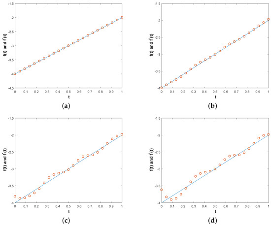
Figure 1. Example 1. In the exact solution $(-)$ and numerical solution $(\circ )$ for $f\left(t\right)$ with three different levels of noise [1%,3%,5%] with $\mathsf{\mu }=[6.89\times {10}^{-5},3.66\times {10}^{-4},8.45\times {10}^{-4}]$ in (b–d), respectively, and with noiseless data (a) with $\mathsf{\mu }=1.00\times {10}^{-9}$, the parameters are $M_1=10,N_1=10,L=20$ and $d_1=d_2=2.5$, and the RMSEs of (a–d) are $[2.8304\times {10}^{-5},0.0199,0.0673,0.1117]$, respectively.

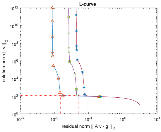
Figure 2. Example 1. The L-curve plot for $\delta =1\%(▵),6.89\times {10}^{-5}$, $\delta =3\%(\square ),3.66\times {10}^{-4}$ and $\delta =5\%(*),8.45\times {10}^{-4}$.

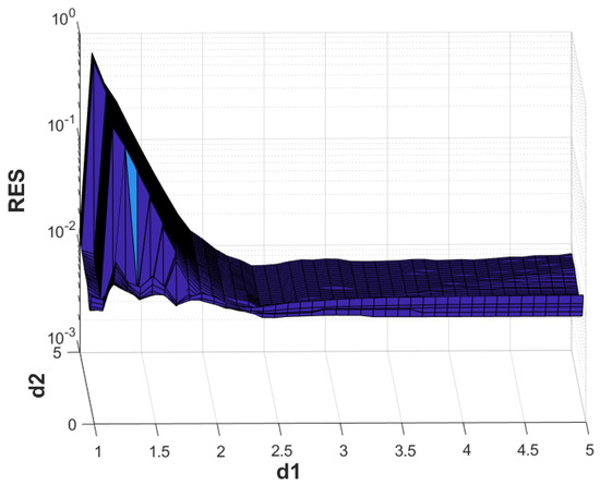
Figure 3. Example 1. The RES for $(d_1,d_2)\in [1,5]\times [1,5]$, $M_1$ = 10, $N_1$ = 10, L = 20 and $\delta =1\%$.

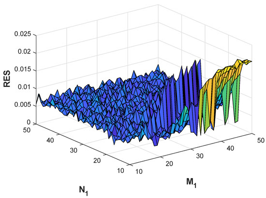
Figure 4. Example 1. The RES for $d_1=d_2=2.5,L=2M_1$, $\delta =1\%$ and $(M_1,N_1)\in [10,50]\times [10,50],M=4M_1$ collocation points and $N=4N_1$ source points.

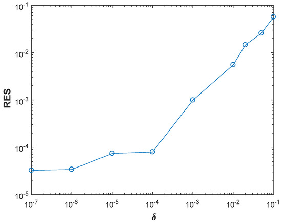
Figure 5. Example 1. RES versus relative noise levels.

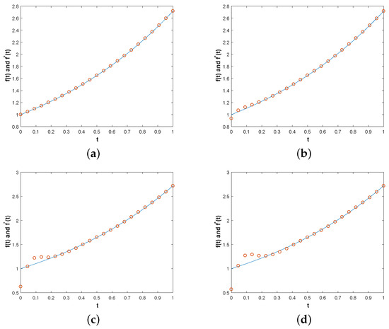
Figure 6. Example 2. In the exact solution $(-)$ and numerical solution $(\circ )$ for $f\left(t\right)$ with three different levels of noise [1%,3%,5%] with $\mathsf{\mu }=[7.04\times {10}^{-4},3.71\times {10}^{-3},5.29\times {10}^{-3}]$ in (b–d), respectively, and with noiseless data (a) with $\mathsf{\mu }=1.00\times {10}^{-9}$, the parameters are $M_1=10,N_1=10,L=20$ and $d_1=d_2=2.5$, and the RMSEs of (a–d) are $[1.1728\times {10}^{-4},0.0160,0.0852,0.1031]$, respectively.

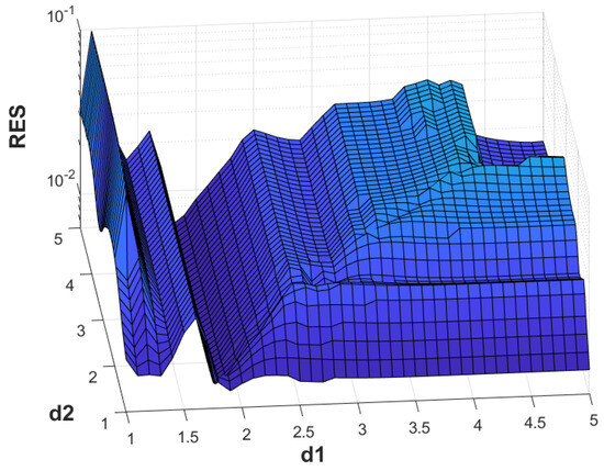
Figure 7. Example 2. The RES for $(d_1,d_2)\in [1,5]\times [1,5]$, $M_1=10,N_1=10,L=20$ and $\delta =1\%$.

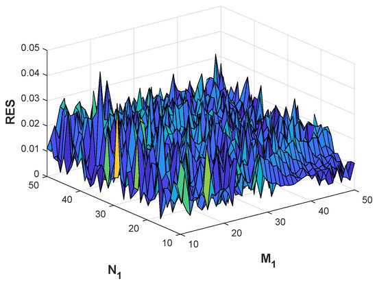
Figure 8. Example 2. The RES for $d_1=d_2=2,L=2M_1$, $\delta =1\%$ and $(M_1,N_1)\in [10,50]\times [10,50],M=4M_1$ collocation points and $N=4N_1$ source points.

Example 2. 

Here we have another example:

$$u(\rho ,t)=e^{-t}{J}_0\left(\rho \right)+e^t,$$

(53)

and

$$f\left(t\right)=e^t.$$

(54)

Example 3. 

We consider another problem given by

$$u(\rho ,t)={\rho }^2+2t+sin\left(2\pi t\right),$$

(55)

and

$$f\left(t\right)=-2+2\pi cos\left(2\pi t\right).$$

(56)

From Table 2, similar conclusions can be observed to those from Table 1.

Table 2. The values of $RES\left(f\right)$ for various of $\delta$ and ${\rho }_1$, $d_1=d_2=2.5$.

${\mathit{\rho }}_1$	$\mathit{\delta }=10\%$	$\mathit{\delta }=5\%$	$\mathit{\delta }=1\%$	$\mathit{\delta }=0.1\%$
0.1	$3.5361\times {10}^{-2}$	$4.4787\times {10}^{-3}$	$2.0455\times {10}^{-3}$	$7.7911\times {10}^{-4}$
0.2	$3.5308\times {10}^{-2}$	$4.4545\times {10}^{-3}$	$1.5426\times {10}^{-3}$	$3.1179\times {10}^{-4}$
0.3	$3.5094\times {10}^{-2}$	$4.3749\times {10}^{-3}$	$8.5922\times {10}^{-4}$	$9.2055\times {10}^{-5}$
0.4	$3.4602\times {10}^{-2}$	$4.1372\times {10}^{-3}$	$5.6661\times {10}^{-4}$	$6.6909\times {10}^{-5}$
0.5	$3.3723\times {10}^{-2}$	$4.1041\times {10}^{-3}$	$5.4701\times {10}^{-4}$	$7.0268\times {10}^{-5}$
0.6	$3.2567\times {10}^{-2}$	$4.1668\times {10}^{-3}$	$6.2040\times {10}^{-4}$	$7.9617\times {10}^{-5}$
0.7	$3.1582\times {10}^{-2}$	$4.3035\times {10}^{-3}$	$6.8345\times {10}^{-4}$	$9.9104\times {10}^{-5}$
0.8	$3.1394\times {10}^{-2}$	$4.7310\times {10}^{-3}$	$7.8702\times {10}^{-4}$	$1.2082\times {10}^{-4}$
0.9	$3.2409\times {10}^{-2}$	$5.7054\times {10}^{-3}$	$9.3945\times {10}^{-4}$	$1.6277\times {10}^{-4}$

As can be seen from Figure 9, Figure 10 and Figure 11, the result of Example 3 is obviously closer to ideal than the previous two examples, and the resulting error is less sensitive to the changes in $d_1,d_2$, $M-N-L$ and $\delta$, which indicates that the stability of the solution can be guaranteed. Numerical experiments show that this method is effective.

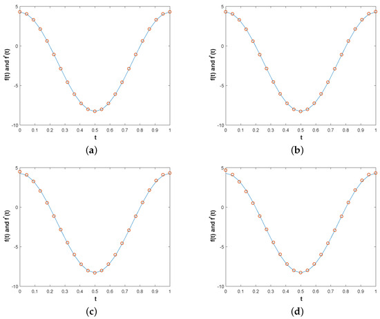
Figure 9. Example 3. In the exact solution $(-)$ and numerical solution $(\circ )$ for $f\left(t\right)$ with three different levels of noise [1%,3%,5%] with $\mathsf{\mu }=[6.89\times {10}^{-5},3.66\times {10}^{-4},8.45\times {10}^{-4}]$ in (b–d), respectively, and with noiseless data (a) with $\mathsf{\mu }=1.00\times {10}^{-9}$, the parameters are $M_1=10,N_1=10,L=20$ and $d_1=d_2=2.5$, and the RMSEs of (a–d) are $[2.8304\times {10}^{-5},0.0199,0.0673,0.1117]$, respectively. Of note are the (a,b) in Figure 9: although there looks to be no difference, they actually are not equal at some point. Because Example 2 is not sensitive to the change in noise data and the change in the noise is small, the change between them is not too large.

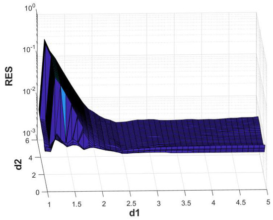
Figure 10. Example 3. The RES for $(d_1,d_2)\in [1,5]\times [1,5]$, $M_1=10,N_1=10,L=20$ and $\delta =1\%$.

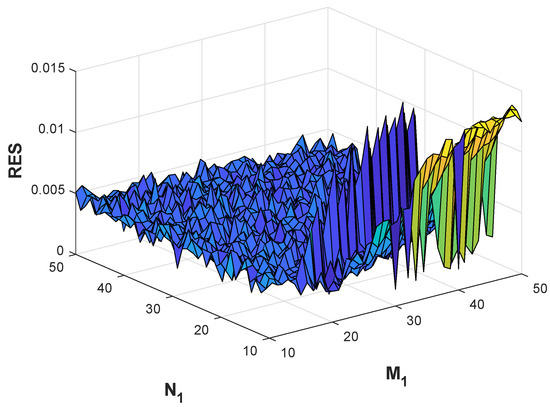
Figure 11. Example 3. The RES for $d_1=d_2=2.5,L=2M_1$, $\delta =1\%$ and $(M_1,N_1)\in [10,50]\times [10,50],M=4M_1$ collocation points and $N=4N_1$ source points.

Example 4. 

We consider the following direct problem:

$$u(\rho ,0)=0,0\le \rho \le 1$$

(57)

$$u(0,t)=0,0\le t\le 1$$

(58)

$$u(1,t)=0,0\le t\le 1$$

(59)

with the heat source function

$$f\left(t\right)=\left\{\begin{array}{cc}-1,\hfill & t\in [0,0.25),\hfill \\ 1,\hfill & t\in [0.25,0.5),\hfill \\ -1,\hfill & t\in [0.5,0.75),\hfill \\ 1,\hfill & t\in [0.75,1].\hfill \end{array}\right.$$

(60)

We solve the problem with MFS, with $M_1=N_1=50,L=100,d_1=d_2=1.3$ when the solution is $u({\rho }_1=0.7,t)=s\left(t\right)$. Then, we use the data $s\left(t\right)$ from the forward problem to solve the inverse problem. Figure 12 shows the comparison between the exact solution and the numerical results. It can be seen from the figure that the numerical approximation is not ideal, but it is reasonably consistent with (60). Compared with the weak relationship between the result and the noise level in Figure 12, it can be seen from Figure 13 that $M-N-L$ has a greater impact on the result. As the value of $M-N-L$ increases, the result becomes closer to ideal.

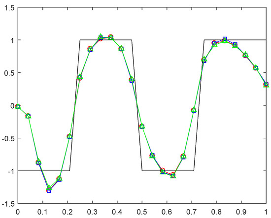
Figure 12. Example 4. The analytical $f\left(t\right)(-)$ and its approximation $f^{*}\left(t\right)$ with $M_1=N_1=26$, $L=52,d_1=d_2=0.8$ and various noise added into the measured data, namely $\delta =1\%(-\circ -),$ $\delta =3\%(-\square -)$ and $\delta =5\%(-▵-)$.

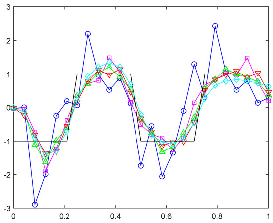
Figure 13. Example 4. The analytical $f\left(t\right)(-)$ and its approximation $f^{*}\left(t\right)$ with $\delta =1\%,d_1=d_2=0.8$ and variable $M-N-L$, namely $M=N=10,L=20(-\circ -),M=N=20,L=40(-\square -),$$M=N=30,L=60(-▵-),M=N=40,L=80(-\nabla -),M=N=50,L=100(-◊-)$.

4.2. Numerical Examples for MFS: Axisymmetric Heat Equation

It can be seen from the analysis in Section 2 that, in this case, the nature of the problem becomes worse, which also increases the difficulty of numerical calculation.

Example 5. 

In this example, the axisymmetric equation is formulated in a solid cylinder with $0<\rho <1$ and $0<h<1$. We use $400collocationpointsand300$ source points to analyze the factors affecting the error of the results at a noise level of $\delta =1\%$. The exact solution is given by

$$u(\rho ,h,t)=({\rho }^2+h^2)+3t^2,0\le \rho \le 1,0\le h\le 1,0\le t\le 1,$$

(61)

and

$$f\left(t\right)=6t-6,0\le t\le 1.$$

(62)

Figure 14 illustrates the relationship between the exact and numerical solution for source $f\left(t\right)$ on $d_{\rho }=3,d_h=5,{\rho }_1=0.1,h_1=0.5$. All the measurement data ${\mathbf{g}}_i$ are computed via the exact solution (3.10). The relationship between $\rho ,h$ and the relative error of the result is shown in Figure 15. Figure 16 considers the relationship between $d_{\rho },d_h$ and the relative error of the result under the condition of ${\rho }_1=0.6$ and $h_1=0.3$.

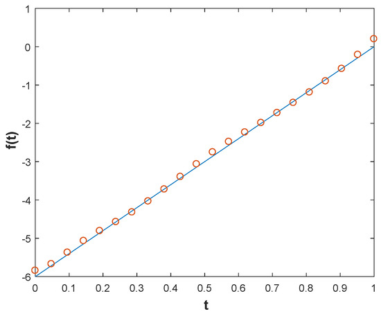
Figure 14. Example 5. In the exact solution $(-)$ and numerical solution $(\circ )$ for source $f\left(t\right)$; we use 400 collocation points and 300 source points, and $d_{\rho }=3,d_h=5,{\rho }_1=0.1,h_1=0.5$, and noise level $\delta =1\%$ with $\mathsf{\mu }=2.18\times {10}^{-5}$, and RMSE is 0.0745.

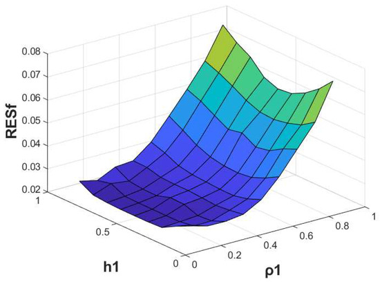
Figure 15. Example 5. The RES for $({\rho }_1,h_1)\in (0.1,0.9)\times (0.1,0.9),d_{\rho }=3,d_h=5$, $M=400,N=300$ and $\delta =1\%$.

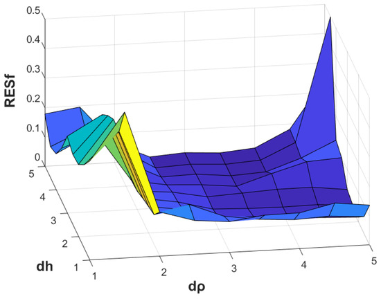
Figure 16. Example 5. The RES for $(d_{\rho },d_h)\in [1,5]\times [1,5],{\rho }_1=0.1,h_1=0.5,M=400,$ $N=300$ and $\delta =1\%$.

Example 6. 

The domain is in a solid cylinder with $0<\rho <1$ and $0<h<1$. The exact solution is given by

$$u(\rho ,h,t)=-1+h+{({\rho }^2+h^2)}^{-1/2}sin\left(\frac{\pi }{4}\sqrt{{\rho }^2+h^2}\right)e^{-{\pi }^{2}t/16}+t{e}^t,0\le \rho \le 1,0\le h\le 1,0\le t\le 1,$$

(63)

and

$$f\left(t\right)=t{e}^t+t,0\le t\le 1.$$

(64)

Figure 17 illustrates the relationship between the exact and numerical solution for source $f\left(t\right)$ on $d_{\rho }=3,d_h=4,{\rho }_1=0.6,h_1=0.3$. Figure 18 and Figure 19 respectively show the relationship between ${\rho }_1,h_1$, $d_{\rho },d_h$ and the relative error of the results. It can be seen that the result is closer to ideal than that of Example 5.

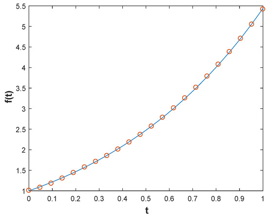
Figure 17. Example 6. In the exact solution $(-)$ and numerical solution $(\circ )$ for source $f\left(t\right)$; we use 400 collocation points and 300 source points, and $d_{\rho }=3,d_h=4,{\rho }_1=0.6,h_1=0.3$, and noise level $\delta =1\%$ with $\mathsf{\mu }=6.49\times {10}^{-5}$, and RMSE is 0.0109.

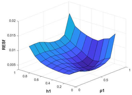
Figure 18. Example 6. The RES for $({\rho }_1,h_1)\in (0.1,0.9)\times (0.1,0.9),d_{\rho }=3,d_h=4$, $M=400,N=300$ and $\delta =1\%$.

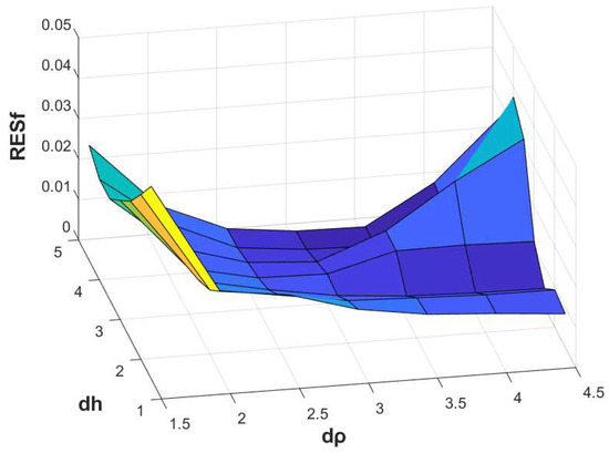
Figure 19. Example 6. The RES for $(d_{\rho },d_h)\in [1.5,4.5]\times [1.5,4.5],{\rho }_1=0.6,h_1=0.3,$ $M=400,N=300$ and $\delta =1\%$.

5. Conclusions

In this paper, we extend MFS to solve the inverse heat source problem, which only varies with time in the radially symmetric and axisymmetric cases. We solve the problem with only one unknown function and introduce the time parameter T, which does not affect the precision of the numerical solution to avoid the singularity. We apply a MFS technique to transform the problem into a discrete system by selecting suitable location source points and matching boundary points, and realize the source term identification of the regional radial symmetry and axisymmetric heat conduction problem based on the Tikhonov regularization method and L-curve criterion. We study several numerical examples of one- and two-dimensional radially symmetric and axisymmetric heat source conduction problems. For one-dimensional cases, we also consider the continuous and discontinuous source terms, respectively. The results show that the proposed method provides an effective and accurate solution for such inverse heat conduction problems.

This method can extend MFS to combine with non-classical regularization methods, which will be accomplished in subsequent works. Secondly, there is no error estimation for solving the inverse source problem for the MSF method combined with Tikhonov regularization, which needs to be studied further.

References

- Kirsch, A. An Introduction to the Mathematical Theory of Inverse Problems; Springer: New York, NY, USA, 2011. [Google Scholar]
- Denisov, A.M. Uniqueness and nonuniqueness of the solution to the problem of determining the source in the heat equation. Comput. Math. Math. Phys. 2016, 56, 1737–1742. [Google Scholar] [CrossRef]
- Yamamoto, M. Conditional stability in determination of force terms of heat equations in a rectangle. Math. Comput. Model. 1993, 18, 79–88. [Google Scholar] [CrossRef]
- Johansson, B.T.; Lesnic, D. Determination of a spacewise dependent heat source. J. Comput. Appl. Math. 2007, 209, 66–80. [Google Scholar] [CrossRef]
- Johansson, B.T.; Lesnic, D. A variational method for identifying a spacewise-dependent heat source. IMA J. Appl. Math. 2007, 72, 748–760. [Google Scholar] [CrossRef]
- Johansson, B.T.; Lesnic, D. A procedure for determining a spacewise dependent heat source and the initial temperature. Appl. Anal. 2008, 87, 265–276. [Google Scholar] [CrossRef]
- Farcas, A.; Lesnic, D. The boundary-element method for the determination of a heat source dependent on one variable. J. Eng. Math. 2006, 54, 375–388. [Google Scholar] [CrossRef]
- Yi, Z.; Murio, D.A. Source term identification in 1-D IHCP. Comput. Math. Appl. 2004, 47, 1921–1933. [Google Scholar] [CrossRef]
- Yi, Z.; Murio, D.A. Source term identification in 2-D IHCP. Comput. Math. Appl. 2004, 47, 1517–1533. [Google Scholar] [CrossRef]
- Yang, C.Y. A sequential method to estimate the strength of the heat source based on symbolic computation. Int. J. Heat Mass. Transfer 1998, 41, 2245–2252. [Google Scholar] [CrossRef]
- Yang, C.Y. Solving the two-dimensional inverse heat source problem through the linear least-squares error method. Int. J. Heat Mass Transfer 1998, 41, 393–398. [Google Scholar] [CrossRef]
- Golberg, M.A.; Chen, C.S. The method of fundamental solutions for potential hemholtz and diffusion problems. In Boundary Integral Methods: Numerical and Mathematical Aspects; Computational Mechanics Publication: Southampton, UK, 1999; pp. 103–176. [Google Scholar]
- Fairweather, G.; Karageorghis, A. The method of fundamental solutions for elliptic boundary value problems. Adv. Comput. Math. 1998, 9, 69–95. [Google Scholar] [CrossRef]
- Powell, M.D.J. Radial basis functions for multivariable interpolation: A review. In Numerical Analysis, Longman Scientific and Technical; Griffiths, D.F., Watson, G.A., Eds.; Longman Scientific and Technical: Harlow, UK, 1987; pp. 223–241. [Google Scholar]
- Kupradze, V.D. A method for the approximate solution of limiting problems in mathematical physics. USSR Comput. Maths. Math. Phys. 1964, 4, 199–205. [Google Scholar] [CrossRef]
- Young, D.L.; Tsai, C.C.; Murugesan, K.; Fan, C.M.; Chen, C.W. Time-dependent fundamental solutions for homogeneous diffusion problems. Eng. Anal. Bound. Elem. 2004, 28, 1463–1473. [Google Scholar] [CrossRef]
- Wu, Z.; Hermite, C. Birkhoff interpolation for scattered data by radial basis function, Approxim. Theory Appl. 1992, 8, 1–10. [Google Scholar]
- Liu, W.K.; Jun, S.; Li, S.; Adee, J.; Belytschko, T. Reproducing kernel particle methods for structural dynamics. Internat. J. Numer. Methods Engrg. 1995, 38, 1655–1679. [Google Scholar] [CrossRef]
- Li, X.; Li, S. Effect of an efficient numerical integration technique on the element-free Galerkin method. Appl. Numer. Math. 2023, 192, 204–225. [Google Scholar] [CrossRef]
- Bogomolny, A. Fundamental solutions method for elliptic boundary value problems. SIAM J. Numer. Anal. 1985, 22, 644–669. [Google Scholar] [CrossRef]
- Chen, J.T.; Chen, I.L.; Chen, K.H.; Lee, Y.T.; Yeh, Y.T. A meshless method for free vibration analysis of circular and rectangular clamped plates using radial basis function. Eng. Anal. Bound. Elem. 2004, 28, 535–545. [Google Scholar] [CrossRef]
- Kang, S.W.; Lee, J.M.; Kang, Y.J. Vibration analysis of arbitrary shape membranes using non-dimensional dynamic influence function. J. Sound Vib. 1999, 221, 117–132. [Google Scholar] [CrossRef]
- Chen, W.; Tanaka, M. A meshless, integration-free, and boundary-only RBF technique. Comput. Math. Appl. 2002, 43, 379–391. [Google Scholar] [CrossRef]
- Chen, W.; Tanaka, M. New insights in boundary-only and domain-type RBF methods. Int. J. Nonlinear Sci. Numer. Simul. 2000, 1, 145–151. [Google Scholar] [CrossRef]
- Chen, W. Singular boundary method: A novel, simple, meshfree, boundary collocation numerical method. Chin. J. Solid Mech. 2009, 30, 592–599. [Google Scholar]
- Fan, C.M.; Huang, Y.K.; Chen, C.S.; Kuo, S.R. Localized method of fundamental solutions for solving two-dimensional Laplace and biharmonic equations. Eng. Anal. Bound. Elem. 2019, 101, 188–197. [Google Scholar] [CrossRef]
- Amin, M.E.; Xiong, X. Source identification problems for radially symmetric and axis-symmetric heat conduction equations. Appl. Numer. Math. 2019, 138, 1–18. [Google Scholar] [CrossRef]
- Shah, R.K.; London, A.L. Laminar Flow Forced Convection in Ducts: A Source Book for Compact Heat Exchanger Analytical Data; Academic Press: Cambridge, MA, USA, 1978. [Google Scholar]
- Rostamzadeh, A. Towards Multidimensional Artificially Characteristic-Based Scheme for Incompressible Thermo-Fluid Problems. Mechanika 2018, 23, 826–834. [Google Scholar] [CrossRef][Green Version]
- Turkyilmazoglu, M.; Duraihem, F.Z. Full Solutions to Flow and Heat Transfer from Slip-Induced Microtube Shapes. Micromachines 2023, 14, 894. [Google Scholar] [CrossRef]
- Hon, Y.C.; Wei, T. A fundamental solution method for inverse heat conduction problem. Eng. Anal. Bound. Elem. 2004, 28, 489–495. [Google Scholar] [CrossRef]
- Hon, Y.C.; Wei, T. Numerical computation for multidimensional inverse heat conduction problem. CMES Comput. Model. Eng. Sci. 2005, 7, 119–132. [Google Scholar]
- Johansson, B.T.; Lesnic, D. A method of fundamental solutions for transient heat conduction. Eng. Anal. Bound. Elem. 2008, 32, 697–703. [Google Scholar] [CrossRef]
- Chantasiriwan, S. Methods of fundamental solutions for time-dependent heat conduction problems. Int. J. Numer. Meth. Eng. 2006, 66, 147–165. [Google Scholar] [CrossRef]
- Yan, L.; Fu, C.L.; Yang, F.L. The method of fundamental solutions for the inverse heat source problem. Eng. Anal. Bound. Elem. 2008, 32, 216–222. [Google Scholar] [CrossRef]
- Wei, T.; Hon, Y.C.; Ling, L. Method of fundamental solutions with regularization techniques for Cauchy problems of elliptic operators. Eng. Anal.Boundary Elem. 2007, 31, 373–385. [Google Scholar] [CrossRef]
- Marin, L.; Lesnic, D. The method of fundamental solutions for the Cauchy problem associated with two-dimensional Helmholtz-type equations. Comput. Struct. 2005, 83, 267–278. [Google Scholar] [CrossRef]
- Marin, L.; Lesnic, D. The method of fundamental solutions for inverse boundary value problems associated with the two-dimensional biharmonic equation. Math. Comput. Model. 2005, 42, 261–278. [Google Scholar] [CrossRef]
- Marin, L.; Lesnic, D. The method of fundamental solutions for nonlinear functionally graded materials. Int. J. Solids Struct. 2007, 44, 6878–6890. [Google Scholar] [CrossRef]
- Hansen, P.C. Rank-Deficient and Discrete Ill-Posed Problems; SIAM: Philadelphia, PA, USA, 1998. [Google Scholar]
- Morozov, V.A. Methods for solving Incorrectly Posed Problems; Springer: New York, NY, USA, 1984. [Google Scholar]
- Engl, H.W.; Hanke, M.; Neubauer, A. Regularization of Inverse Problems, Mathematics, and Its Applications; Kluwer Academic Publishers: Dordrecht, The Netherlands, 1996; Volume 357. [Google Scholar]
- Tautenhahn, U.; Hämarik, U. The use of monotonicity for choosing the regularization parameter in ill-posed problems. Inverse Probl. 1999, 15, 1487–1505. [Google Scholar] [CrossRef]
- Golub, G.; Heath, M.; Wahba, G. Generalized cross-validation as a method for choosing a good ridge parameter. Technometrics 1979, 21, 215–223. [Google Scholar] [CrossRef]
- Wei, T.; Hon, Y.C. Numerical differentiation by radial basis functions approximation. Adv. Comput. Math. 2007, 27, 247–272. [Google Scholar] [CrossRef]
Disclaimer/Publisher’s Note: The statements, opinions and data contained in all publications are solely those of the individual author(s) and contributor(s) and not of MDPI and/or the editor(s). MDPI and/or the editor(s) disclaim responsibility for any injury to people or property resulting from any ideas, methods, instructions or products referred to in the content. |
© 2024 by the authors. Licensee MDPI, Basel, Switzerland. This article is an open access article distributed under the terms and conditions of the Creative Commons Attribution (CC BY) license (https://creativecommons.org/licenses/by/4.0/).