Research on CFRP Defects Recognition and Localization Based on Metamaterial Sensors

Abstract

In the paper, the concept of symmetry is utilized to detect internal defects in Carbon fiber reinforced polymer (CFRP), that is, the reconstruction and localization methods for internal defects in CFRP are symmetrical. CFRP is widely used in industrial, biological and other fields. When there are defects inside the composite materials, its dielectric constant, magnetic permeability, etc. change. Therefore, metamaterial sensors are widely used in non-destructive testing of CFRP Defects. This paper proposes a defect identification and location method based on principal component analysis (PCA) and support vector machine (SVM). The trained model is used to classify the dimensionally reduced data, and the reconstructed defect binary image is obtained. Simulation and physical experiment results show that the method used in this article can effectively identify and locate defects in carbon fiber composite materials.

1. Introduction

With the rapid progress of science and technology, CFRP has become an indispensable material in the industrial field, especially the aerospace field, due to its properties such as lightness, high stiffness, fatigue resistance and pressure resistance. The popularity of CFRP has brought about an urgent need for its safety. However, defects can occur in carbon fiber composites during the manufacturing process and use. Therefore, defect detection of composite materials is of great significance. In the industry, commonly used non-destructive testing technologies include ultrasonic testing, eddy current testing, thermal imaging testing and microwave testing. However, ultrasonic testing cannot penetrate highly porous materials and is limited by coupling agents, while also requiring extensive data interaction. Eddy current testing is widely used for surface crack and corrosion detection, but due to the penetration limitations of low-frequency electromagnetic waves, it is not effective when detecting low-loss dielectric materials.

A variety of microwave non-destructive testing technologies for composite material testing have been reported [1]. Although some promising results have been achieved, traditional microwave technologies still face some challenges, including high data complexity, space Poor image quality and blurry defect shapes, etc. Distance changes and optimal frequency selection can cause these problems, which in turn reduce the geometric measurement accuracy of defects [2]. Therefore, artificial intelligence technology is used in microwave non-destructive testing to solve the challenges based on microwave technology. Since machine learning technology has high capabilities in training and solving complex and nonlinear data, the ability to accurately classify defective and defect-free areas using machine learning classifiers will be reflected in measurement accuracy. Therefore, the use of intelligent classifiers can process and detect raw data while ensuring reliability and speed [3], and at the same time, it can improve the resolution of defect detection while automating the processing process [4]. In addition, artificial intelligence can solve the complexity problem when collecting data through non-linear classification [5].

An earlier attempt was made in [6] to introduce intelligent microwave non-destructive testing, using a combination of SVM and Artificial Neural Network (ANN) classifiers to find small changes in reflection coefficients. A corrosion defect imaging system using microwave sensors and AI models was implemented in [7]. Feature extraction is performed using the supervised PCA algorithm. Implement artificial intelligence model through SVM algorithm. The trained model shows good generalization ability in defect representation. Frequency sweep-based features will lead to an increase in the amount of operations and calculations, and are very time-consuming in the initial stage of inspection, so machine learning feature selection is used in [8] to reduce the sweep frequency. Furthermore [9] developed and implemented an image gradient-based feature extraction method that includes a filter-based method and parameters from Weibull fitting. Liu et al. proposed a new loss function design that incorporates multiple scattering using near-field quantities to reconstruct the dielectric constant [10].

This paper is based on the non-destructive testing of CFRP using metamaterial sensors, studies defect identification and positioning technology, and proposes defect identification and positioning technology based on principal component analysis and support vector machines. Use a metamaterial sensor to conduct two-dimensional plane scanning of composite materials, and use principal component analysis to reduce the dimensionality of the original scan data obtained; then use a support vector machine to train the dimensionally reduced data with labels to obtain a classification model. Finally, the trained model is used to perform binary classification of defect-free and defective experimental data, and the reconstructed defect binary image is obtained, finally realizing the identification and positioning of defects.

2. Equivalent Model

2.1. Conductivity

Typically, research generally agrees that unidirectional carbon fiber composite laminates have anisotropic electrical properties. That is, the conductivity along the direction perpendicular to the fibers is relatively small, while the conductivity of the composite along the fiber direction can be calculated using the fiber volume fraction and the total single fiber conductivity. For an ideal unidirectional composite, the composite conductivity ${\sigma }_{cp}$ parallel to the fibers can be calculated as:

$${\sigma }_{cp}={\sigma }_f/v_f$$

(1)

where $v_f$ is the volume fraction of the fiber; ${\sigma }_f$ is the conductivity of the carbon fiber. If the conductivity in all three directions is considered, the conductivity tensor of the carbon fiber composite plate can be expressed as:

$$\left[\sigma \right]=\left[\begin{array}{ccc}{\sigma }_l{\cos }^2\theta +{\sigma }_t{\sin }^2\theta & \left({\sigma }_l-{\sigma }_t\right)/2\cdot \sin 2\theta & 0\\ \left({\sigma }_l-{\sigma }_t\right)/2\cdot \sin 2\theta & {\sigma }_l{\cos }^2\theta +{\sigma }_t{\sin }^2\theta & 0\\ 0& 0& {\sigma }_{cp}\end{array}\right]$$

(2)

where ${\sigma }_l$ represents the longitudinal conductivity of the layer; ${\sigma }_t$ represents the transverse conductivity of the layer; ${\sigma }_{cp}$ is the cross-layer conductivity; $\theta$ represents the direction of each ply.

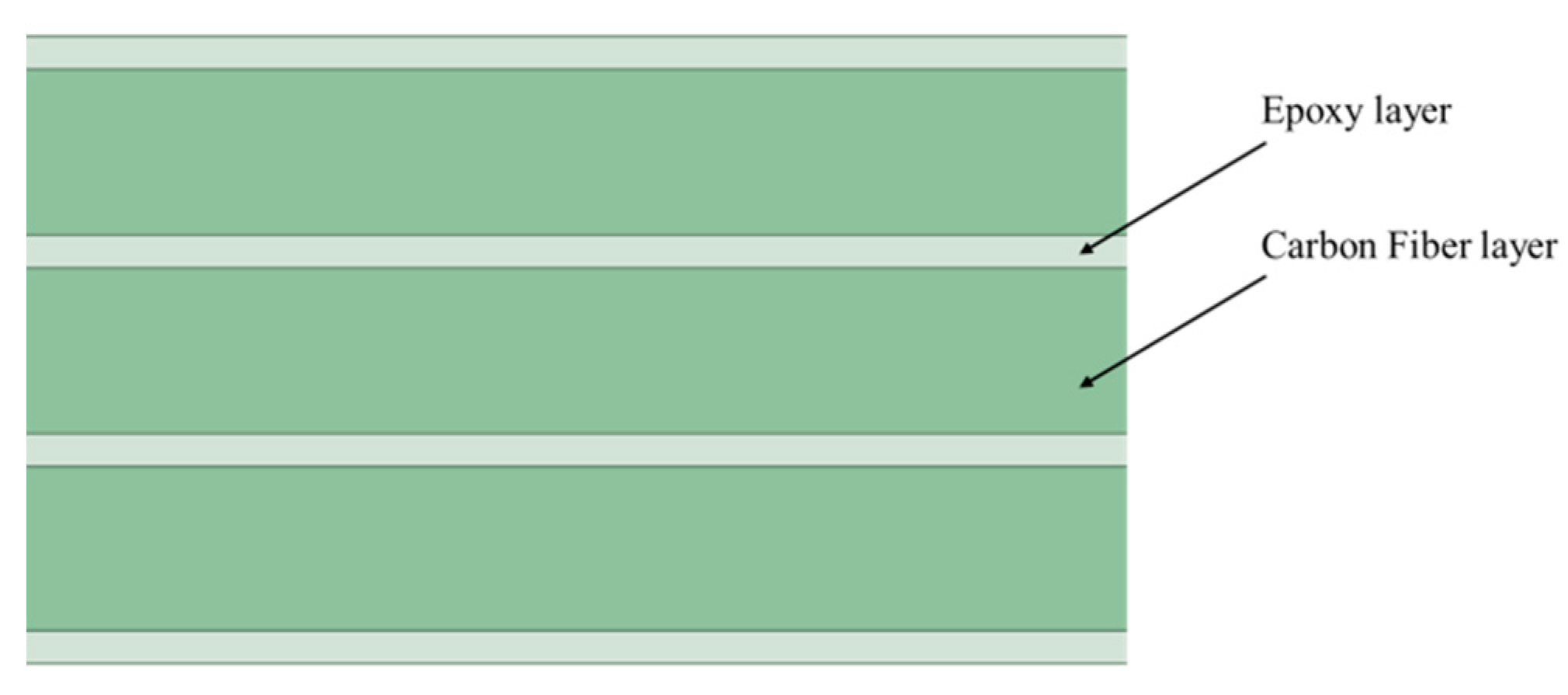
2.2. Three-Layer Uniform Model

The characteristic of the three-layer uniform model [11] is that the dielectric coefficient ${\epsilon }_{eff}$ of the central layer is constant throughout the layer. When microwaves propagate into fiber composite panels, they pass through three separate zones. The microwaves enter the panel first and see a uniform layer. This layer has constant material properties corresponding to the material properties of the matrix or resin surrounding the fibers. The thickness t of this layer corresponds to the distance from the edge of the panel to the edge of the fiber, and its dielectric coefficient is $\epsilon$. The central layer is the fiber layer. The wave finally enters the uniform layer again, which is the same as the first layer (i.e., constant material properties $\epsilon$ and thickness $t$). At any given cross-section in the uniform layer, the material properties approximate the effective material properties of the periodic laminate media shown in Figure 1.

Figure 1. Simulation model of carbon fiber composite materials.

This type of medium behaves like an anisotropic but homogeneous material with the following tensor permittivity and magnetic permeability:

$$\left[\epsilon \right]=\left[\begin{array}{ccc}{\epsilon }_x& 0& 0\\ 0& {\epsilon }_y& 0\\ 0& 0& {\epsilon }_z\end{array}\right]$$

(3)

$$\left[\mu \right]=\left[\begin{array}{ccc}{\mu }_x& 0& 0\\ 0& {\mu }_y& 0\\ 0& 0& {\mu }_z\end{array}\right]$$

(4)

where:

$${\epsilon }_x^{-1}=\left(1-g\right){\epsilon }_a^{-1}+g{\epsilon }_b^{-1}$$

(5)

$${\mu }_x^{-1}=\left(1-g\right){\mu }_a^{-1}+g{\mu }_b^{-1}$$

(6)

$${\epsilon }_y={\epsilon }_z=\left(1-g\right){\epsilon }_a+g{\epsilon }_b$$

(7)

$${\mu }_y={\mu }_z=\left(1-g\right){\mu }_a+g{\mu }_b$$

(8)

where ${\epsilon }_a$ represents the dielectric constant of the epoxy resin matrix, ${\mu }_a$ indicates the magnetic permeability of the epoxy resin matrix, ${\epsilon }_b$ representing the dielectric constant of carbon fiber,${\mu }_b$ indicates the magnetic permeability of carbon fiber, $g$ is the relative spatial volume occupied by carbon fiber materials.

Fiber composite panels are structures composed of fibers aligned in only one direction, embedded in the center of a matrix or resin. Some of the composite structures analyzed here consist of two or more multilayer panels. Typically, the fibers in each panel of a composite structure can be oriented in different directions. Considering a multi-panel composite structure, when a three-layer model is used for this multi-panel structure, then each panel will be represented by three layers. Therefore, the multi-panel composite will have a periodic arrangement with carbon fiber and epoxy layers interlaced as shown in the model shown in Figure 1. The light-colored part is the epoxy resin layer, and the dark-colored part is the carbon fiber layer. Its structure shows periodic characteristics.

2.3. Carbon Fiber Composite Structural Analysis

This paper established a carbon fiber composite structure simulation model in High Frequency Structure Simulator (HFSS). The simulation model is shown in Figure 2. The composite material equivalent simulation model adopts a three-layer uniform model. Figure 2 shows the overall simulation model of carbon fiber composite material. Figure 1 shows the side view of carbon fiber composite material, that is, the layering situation of the composite material. It can be seen from the figure that each layer of material is mainly composed of carbon fiber layer and FR4 epoxy resin plate. Carbon fiber and FR4 epoxy resin plates are alternately arranged to form the overall simulation structure of carbon fiber composite materials. The materials of each layer of the model and their laying angles are shown in Table 1. Considering that in carbon fiber composite materials, different layers of carbon fibers are anisotropic, in the simulation model, different layers of carbon fibers are laid at different angles, namely along the x-axis and along the y-axis.

Figure 2. Carbon fiber composite overall simulation model.

Table 1. Model Ply Material and Laying Angle.

Number of Layers	Material Name	Laying Angle
1	epoxy	non
2	carbon fiber	0
3	epoxy	non
4	carbon fiber	90
5	epoxy	non
6	carbon fiber	0
7	epoxy	non

3. Methods of Defect Identification and Location

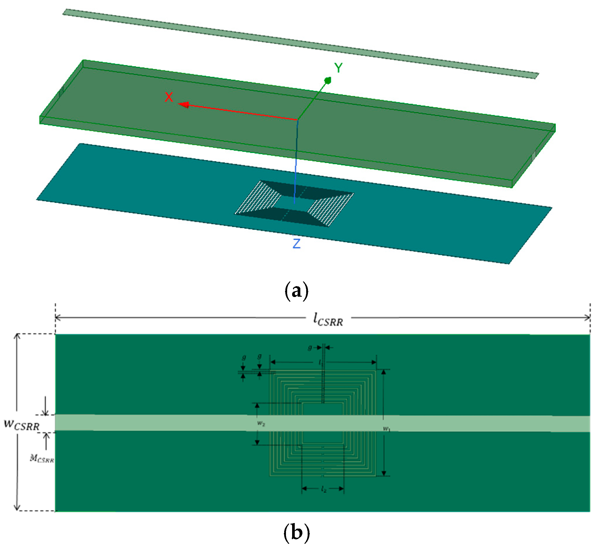
3.1. Analysis of Non-Destructive Testing of Resonant Sensors

Microwave resonance sensors utilize the propagation characteristics of microwaves to achieve detection by detecting the interaction between the target to be measured and the sensor. The sensor works in the microwave frequency range. When there is a defect in the target to be measured, it will affect the distribution of the field near the resonant sensing structure, causing changes in the relevant parameters of the sensing structure. Generally, it is reflected in the scattering parameter amplitude and resonance frequency. influence, thereby realizing the detection of the target to be tested. The detection schematic diagram is shown in Figure 3. Typically, the behavior of a resonant structure can be equivalent to a resonant circuit. In resonant sensor detection, if there are defects in the material being tested, the defects will affect the resonant sensing structure, causing the equivalent circuit of the original resonant sensing structure to change. After excitation of the resonant sensing structure using a two-port network, the changes caused by defects can be converted into detectable observations, such as the resonant frequency of the scattering parameters and their resonance amplitude.

Figure 3. Schematic diagram of resonance sensor detection.

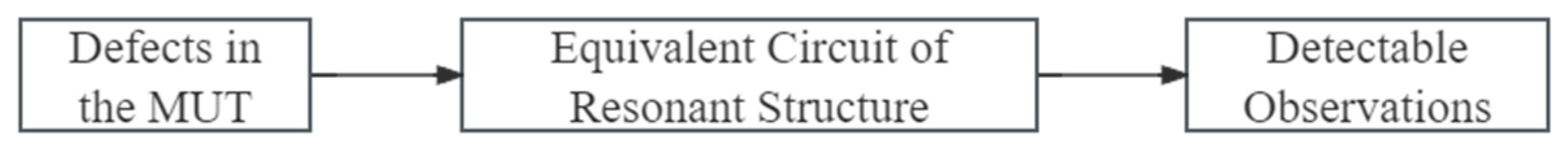
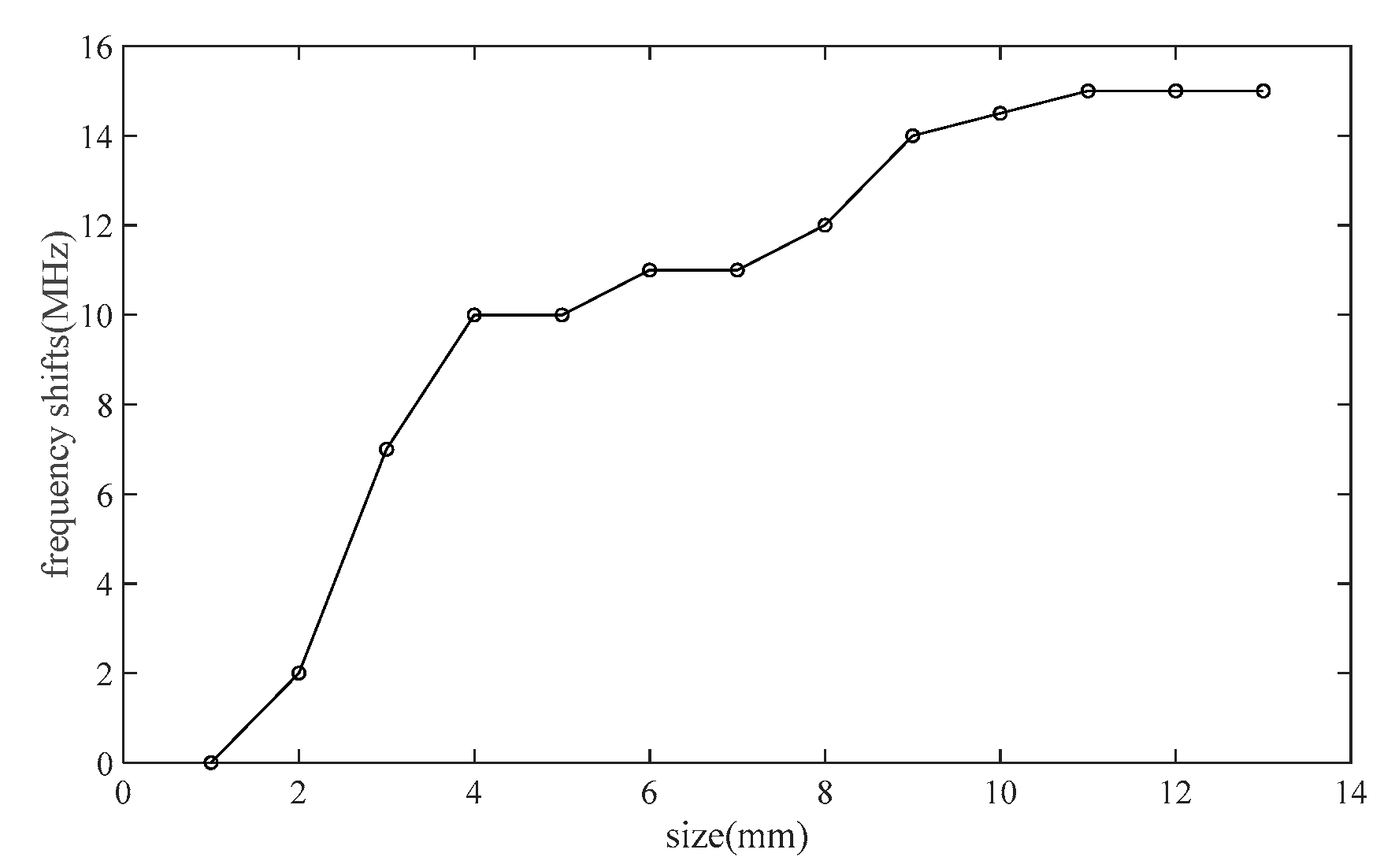
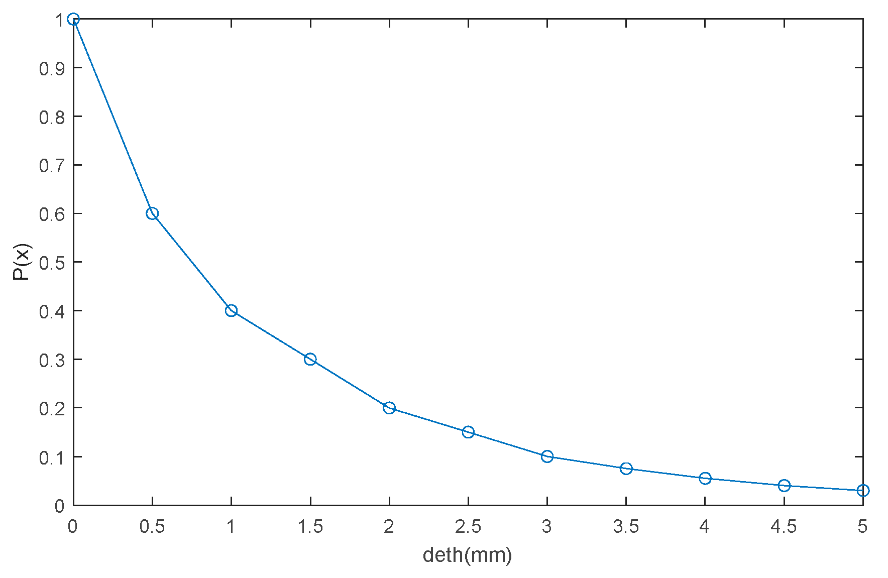
3.2. Analysis of the Impact of Defects on Resonant Sensors

Assume that before defects are introduced in the resonant cavity, let ${\epsilon }_0$ and ${\mu }_0$ represent the dielectric constant and magnetic permeability of the resonant cavity in the initial state, ${\mathit{E}}_0$ and ${\mathit{H}}_0$ represent the electric field and magnetic field respectively before the defects are introduced, and ${\omega }_0$ represents the initial state of the resonant cavity. Resonant frequency, $V_0$ represents the volume of the resonant cavity and $S_0$ represents the inner surface area of the resonant cavity; when introducing the target to be measured, let ${\epsilon }_m$ and ${\mu }_m$ represent the relative dielectric constant and relative permeability of the target to be measured respectively, and its volume is $V_m$; After introducing the perturbation of defects in the target to be measured, let ${\epsilon }_m+∆\epsilon$ and ${\mu }_m+∆\mu$ represent the relative permittivity and relative permeability of the defects in the target to be measured respectively, and the defect volume is $V_d$. At this time, the electric field and magnetic field in the resonant cavity become ${\mathit{E}}_1$ and ${\mathit{H}}_1$ respectively, and the resonant frequency becomes ${\omega }_1$. Then the resonant frequencies ${\omega }_0$ and ${\omega }_1$ have the following relationship before and after introducing defect disturbance:

$$\begin{array}{l}{\displaystyle \frac{{\omega }_1-{\omega }_0}{{\omega }_1}}=\\ {\displaystyle \frac{{\displaystyle {\iiint }_{V_d}\left(\Delta \epsilon {\mathit{E}}_1\cdot {\mathit{E}}_0^{\ast }+\Delta \mu {\mathit{H}}_1\cdot {\mathit{H}}_0^{\ast }\right)}dV}{{\displaystyle {\iiint }_{V_0-V_m}\left({\epsilon }_0{\mathit{E}}_1\cdot {\mathit{E}}_0^{\ast }+{\mu }_0{\mathit{H}}_1\cdot {\mathit{H}}_0^{\ast }\right)}dV+{\displaystyle {\iiint }_{V_m}\left({\epsilon }_m{\mathit{E}}_1\cdot {\mathit{E}}_0^{\ast }+{\mu }_m{\mathit{H}}_1\cdot {\mathit{H}}_0^{\ast }\right)}dV}}\end{array}$$

(9)

Generally speaking, assuming that the changes in the dielectric constant and magnetic permeability of the resonant cavity after being affected by defects are relatively small, that is, $∆\epsilon$ and $∆\mu$ are relatively small, the electric and magnetic fields ${\mathit{E}}_0$ and ${\mathit{H}}_0$ of the original resonant cavity can be used to approximately replace ${\mathit{E}}_1$ and ${\mathit{H}}_1$, so the above formula can be rewritten as:

$$\begin{array}{l}{\displaystyle \frac{{\omega }_1-{\omega }_0}{{\omega }_1}}=\\ {\displaystyle \frac{{\displaystyle {\iiint }_{V_d}\left(\Delta \epsilon {\left|{\mathit{E}}_0\right|}^2+\Delta \mu {\left|{\mathit{H}}_0\right|}^2\right)}dV}{{\displaystyle {\iiint }_{V_0-V_m}\left({\epsilon }_0{\left|{\mathit{E}}_0\right|}^2+{\mu }_0{\left|{\mathit{H}}_0\right|}^2\right)}dV+{\displaystyle {\iiint }_{V_m}\left({\epsilon }_m{\left|{\mathit{E}}_0\right|}^2+{\mu }_m{\left|{\mathit{H}}_0\right|}^2\right)}dV}}\end{array}$$

(10)

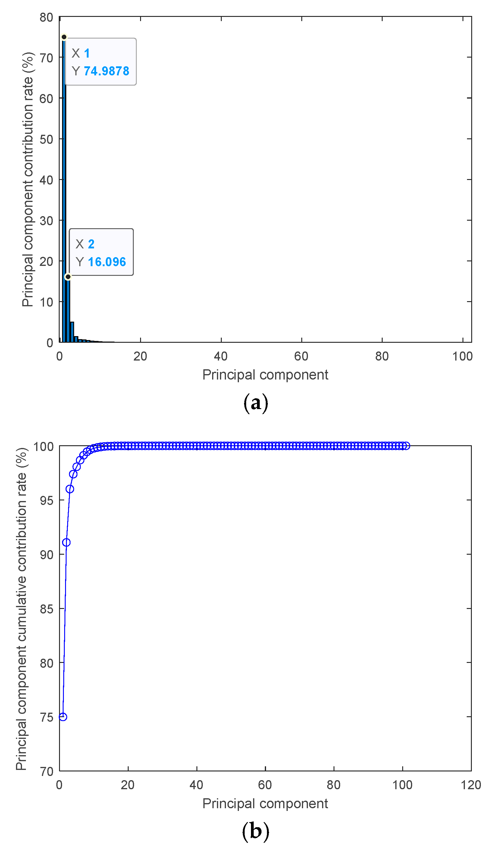
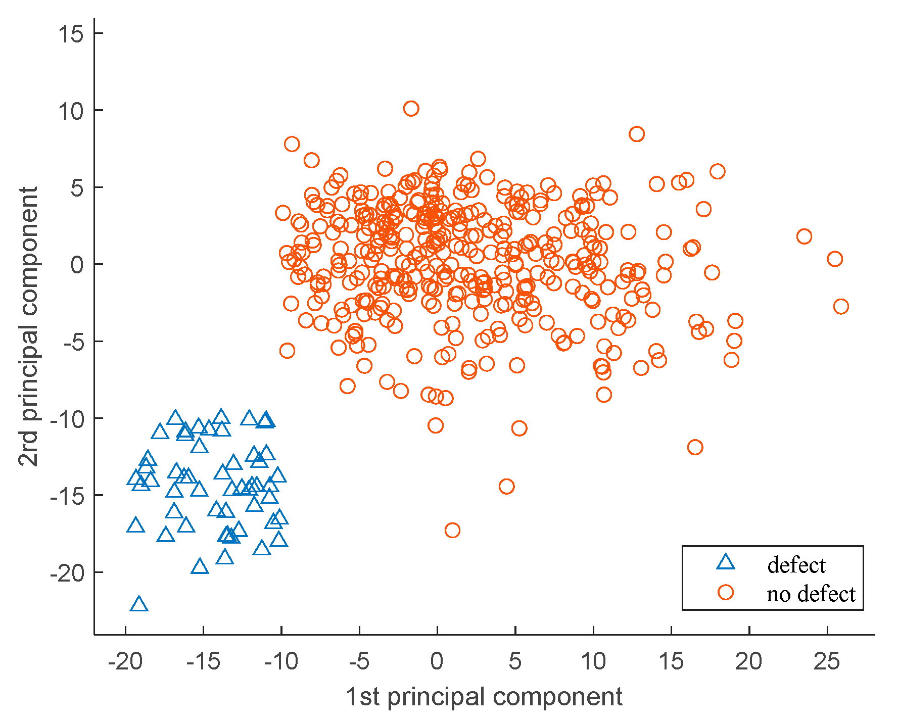
3.3. Principal Component Analysis

The algorithm flow of principal component analysis mainly consists of the following steps:

(1)

The original data set is formed into a matrix $X$ with $n$ rows and $m$ columns by column, indicating that the data set contains $n$ samples, and each sample contains $m$ variables;

(2)

Demean each row (i.e., each sample) of the data set X, that is, subtract the mean of the current row, $\tilde{X}=X-\overline{X}=X-\sum _{i=1}^m{x}_i/n$;

(3)

Solve the covariance matrix $V$ of the demeaned matrix $\tilde{X}$, $V=\tilde{X}{\tilde{X}}^T/n$;

(4)

Solve the eigenvalue ${\lambda }_i$ of the covariance matrix $V$ and its corresponding eigenvector $w_i$;

(5)

Arrange the eigenvectors into a new matrix according to the size of the eigenvalues, and take the eigenvectors corresponding to the first $k$ eigenvalues $\mathsf{\Lambda }=\mathrm{d}\mathrm{i}\mathrm{a}\mathrm{g}\left[{\lambda }_1,{\lambda }_2,\cdots ,{\lambda }_k\right]$ as the basis of the submatrix, that is, the matrix of the required k principal component is $P=W_d^T\tilde{X}$;

(6)

The data set $X=WP+\overline{X}$ is reconstructed based on the extracted $k$ principal components, which achieves data dimensionality reduction.

Figure 4 shows the contribution rate of each principal component obtained by using PCA to process the original data obtained by scanning the measured material with the sensor, and the cumulative contribution rate of the principal components obtained by ranking according to the contribution rate. The original data is frequency sweep data with a frequency sweep range of 0.5 GHz to 1 GHz, that is, the $S_{21}$ amplitude of each frequency point. As can be seen from the figure, after PCA processing of the original data, the contribution rate of the first principal component is 74.9878%, the contribution rate of the second principal component is 16.096%, and the cumulative contribution rate of the first two principal components reached 91.0838%. The contribution rate up to the 23rd principal component can be basically ignored. Therefore, using PCA can realize feature extraction of the original data and characterize the original data without losing too much information.

Figure 4. (a) The contribution rate of each principal component; (b) Principal component cumulative contribution rate based on contribution rate arrangement.

3.4. Support Vector Machine Classifier

In order to obtain the model, the first step is to collect data. This article uses sensors to obtain frequency sweep data of the tested material, and then uses PCA to reduce the dimension. Then the data set is divided into a training set and a test set, and the data is classified. Unification; the next step is to choose an appropriate kernel function. The quadratic polynomial kernel function used in this article is. At the same time, cross-validation is used to find the best parameters $C$ and $\xi$; then the best parameters $C$ and $\xi$ are used to train the entire training set to derive the model.

The SVM model, which uses a quadratic polynomial as the kernel function, classifies two types of problems, and the results are shown in Figure 5. Figure 5 is obtained from an SVM classifier applied to data reduction, providing a visual image of the learned two-dimensional model. Defective scans (red circles) and defective scans (blue triangles) are classified.

Figure 5. Decision result.

4. Experiments and Results

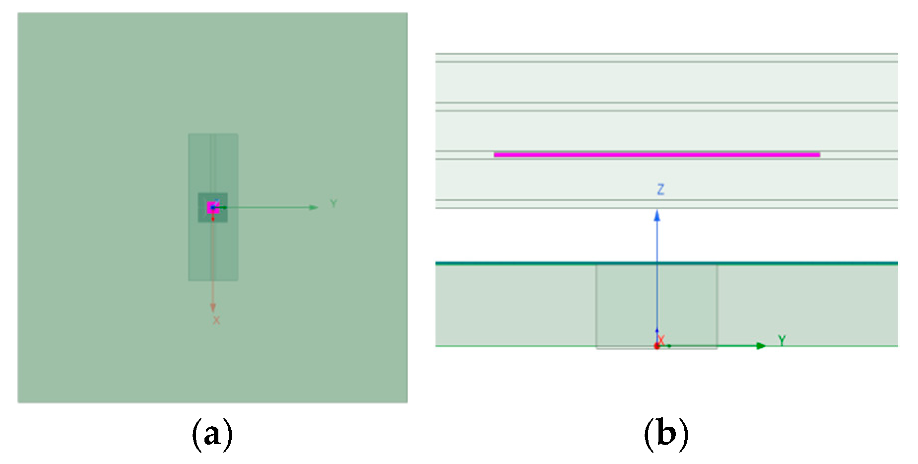
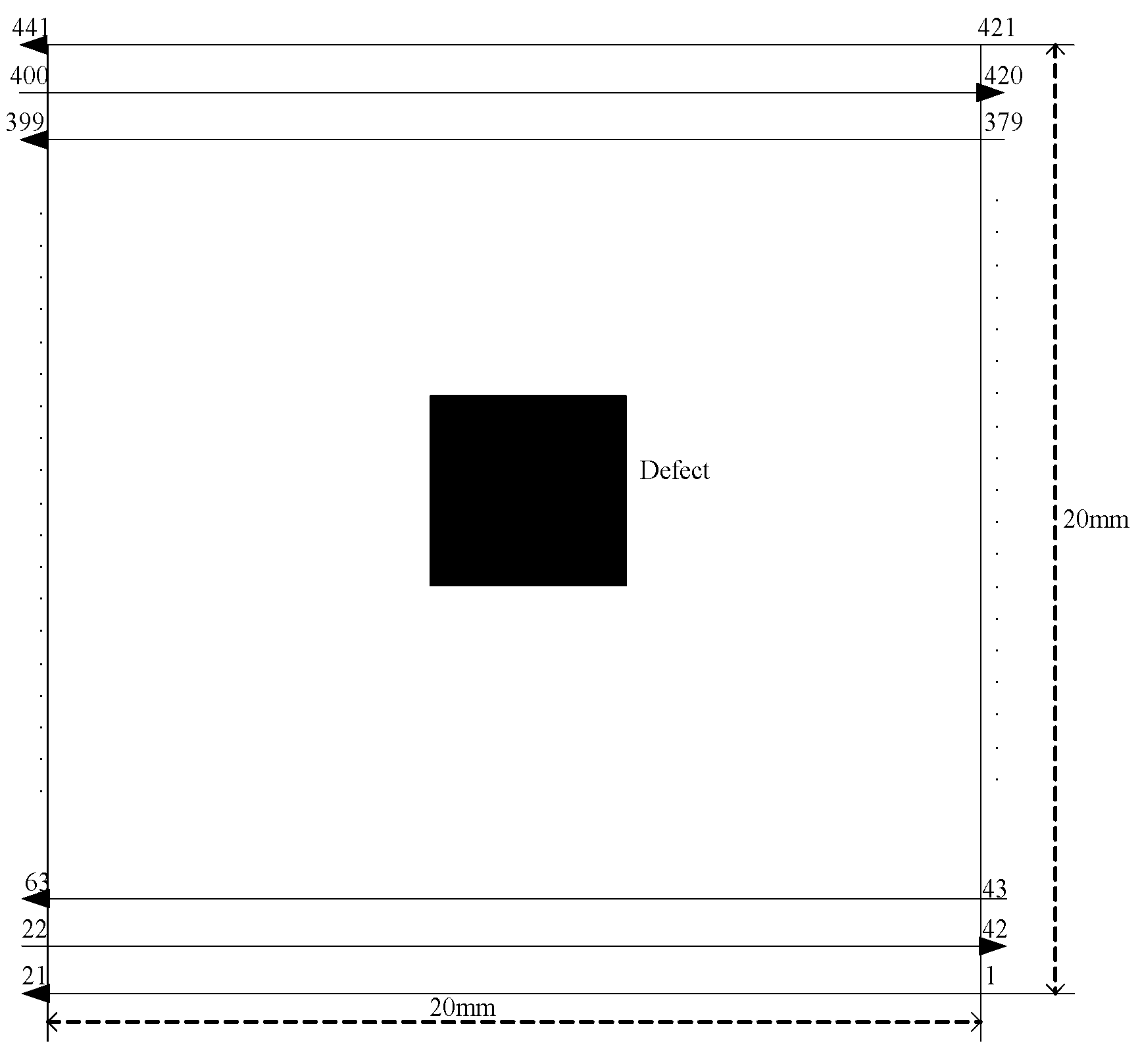
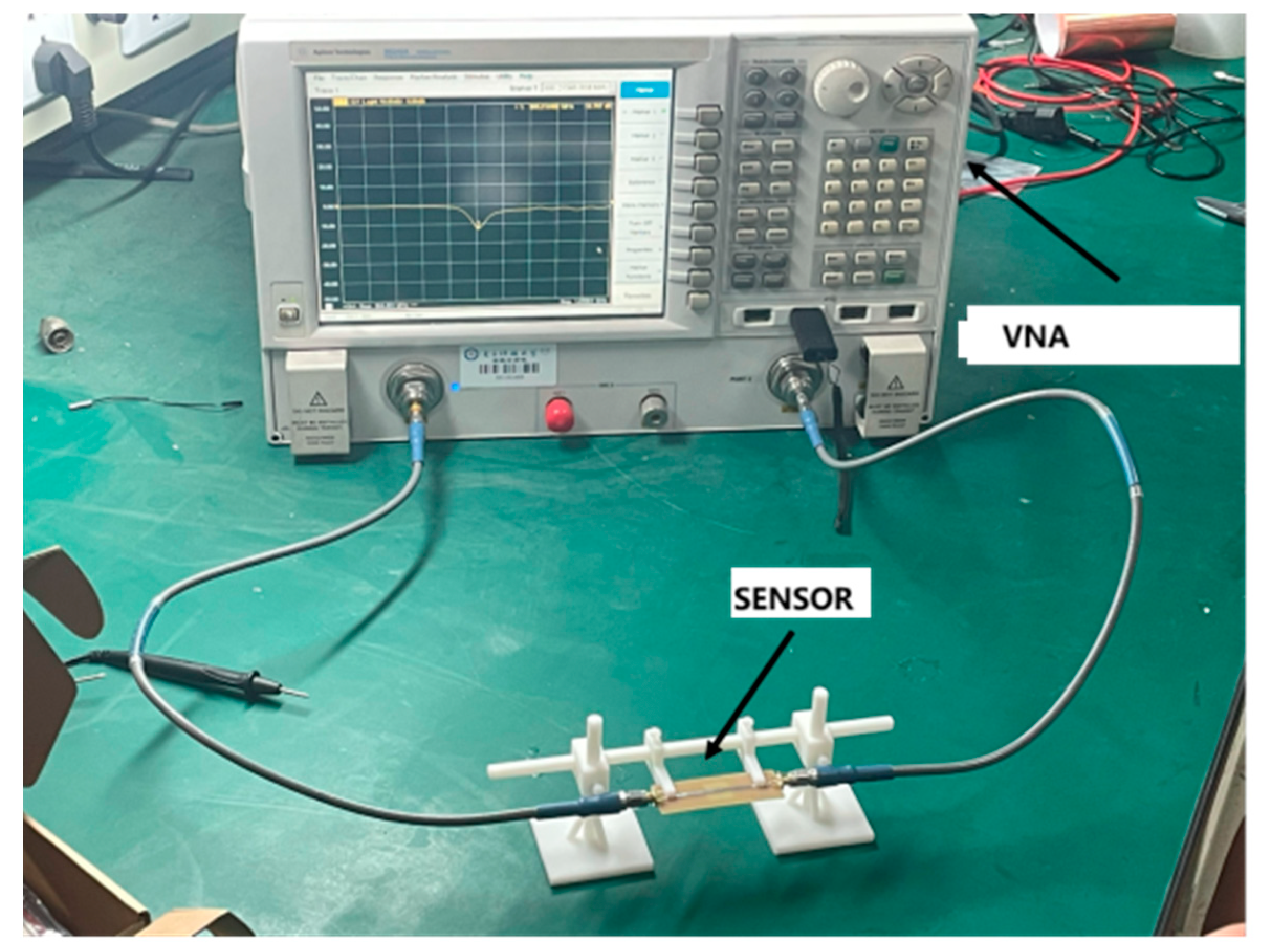
4.1. Sensor Settings

The resonant sensing structure of the metamaterial sensor is shown in Figure 6a, which consists of nested Complimentary Split Resonant Ring (CSRR) etched on the ground plate of the microstrip transmission line and wave ports at both ends, combined to form a dual port sensor model. The sensing structure uses nested CSRR. Load CSRR on a grounding copper plane with a thickness of 35 μm, using a 0.1 mm thick FR4 epoxy resin board as the substrate. The top plane includes a 1.86 mm wide microwave transmission line as the electromagnetic field source between ports 1 and 2. Figure 6b illustrates the setup of the resonant sensing structure model embedded with CSRR. In the CSRR unit structure, $l_1=w_1=$12 mm, $l_2=w_2=$ 4.4 mm, and g = 0.2 mm. The length of the base $l_{CSRR}$ is 60 mm, and the width $l_{CSRR}$ is 20 mm. Using HFSS simulation to verify the defect detection capability of technique. The simulation results are shown in Figure 7 and Figure 8. Figure 7 indicates that defect size of 1 mm or smaller cannot be detected, resulting in zero shift in the sensor’s resonant frequency. Figure 8 shows that when the detection depth is 5 mm, the energy density decreases to 10%.

Figure 6. (a) Resonant sensing structure; (b) Structural parameter settings.

Figure 7. Relationship between resonant frequency shift and defect size.

Figure 8. Relationship between energy attenuation and depth.

According to the above analysis, the defect detection accuracy of this method is 2 mm, and the detection depth can reach 5 mm. The comparison with traditional ultrasound and eddy current testing is shown in Table 2. This method has high detection accuracy, high computational efficiency, and moderate detection depth.

Table 2. Comparison between this method and other methods.

Testing Method	Defect Detection Accuracy	Defect Detection Depth	Computational Efficiency
Ultrasonic testing [12]	3 mm	10 mm	Moderate
eddy current testing [13,14]	6 mm	2 mm	Lower
The method	2 mm	5 mm	Higher

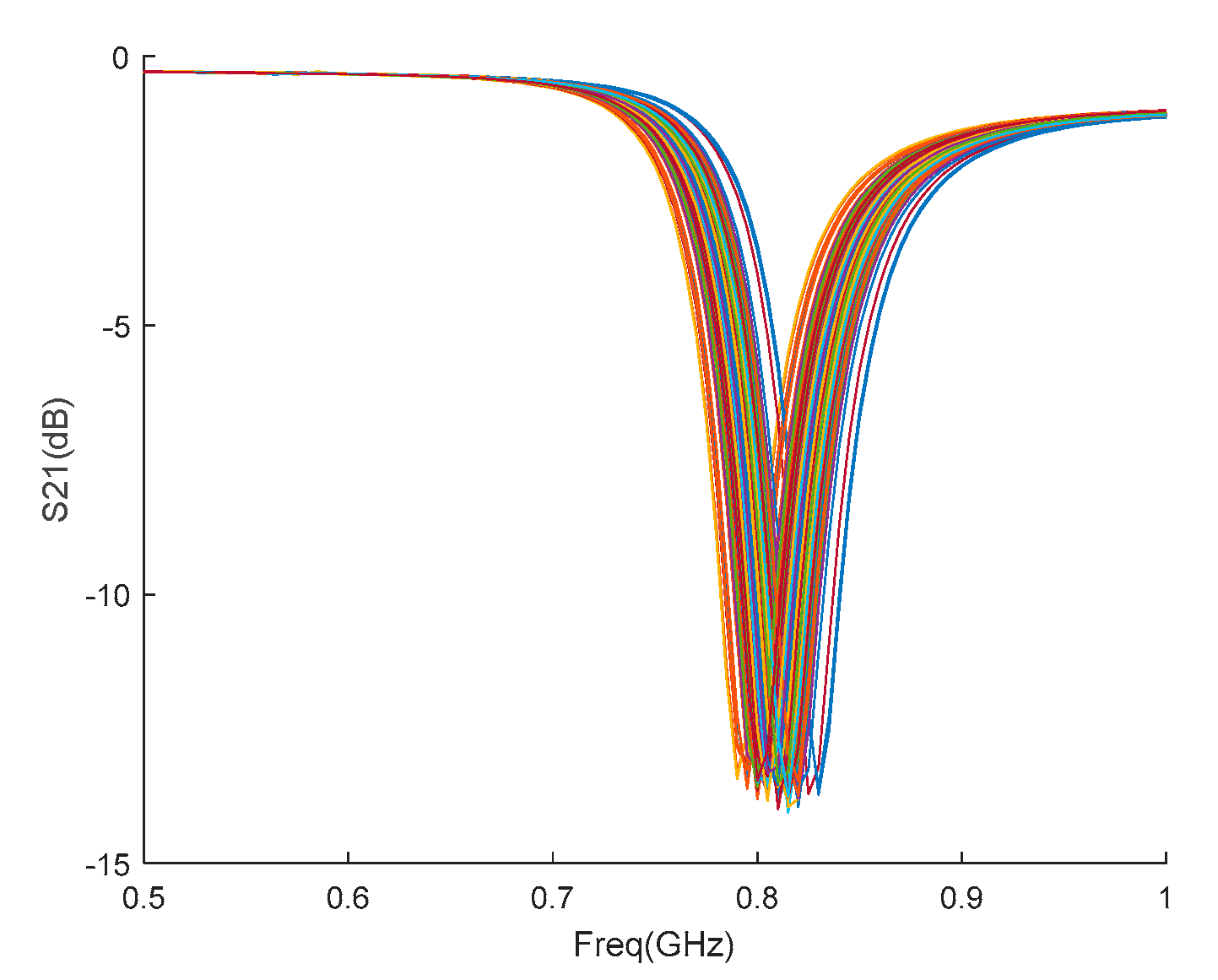
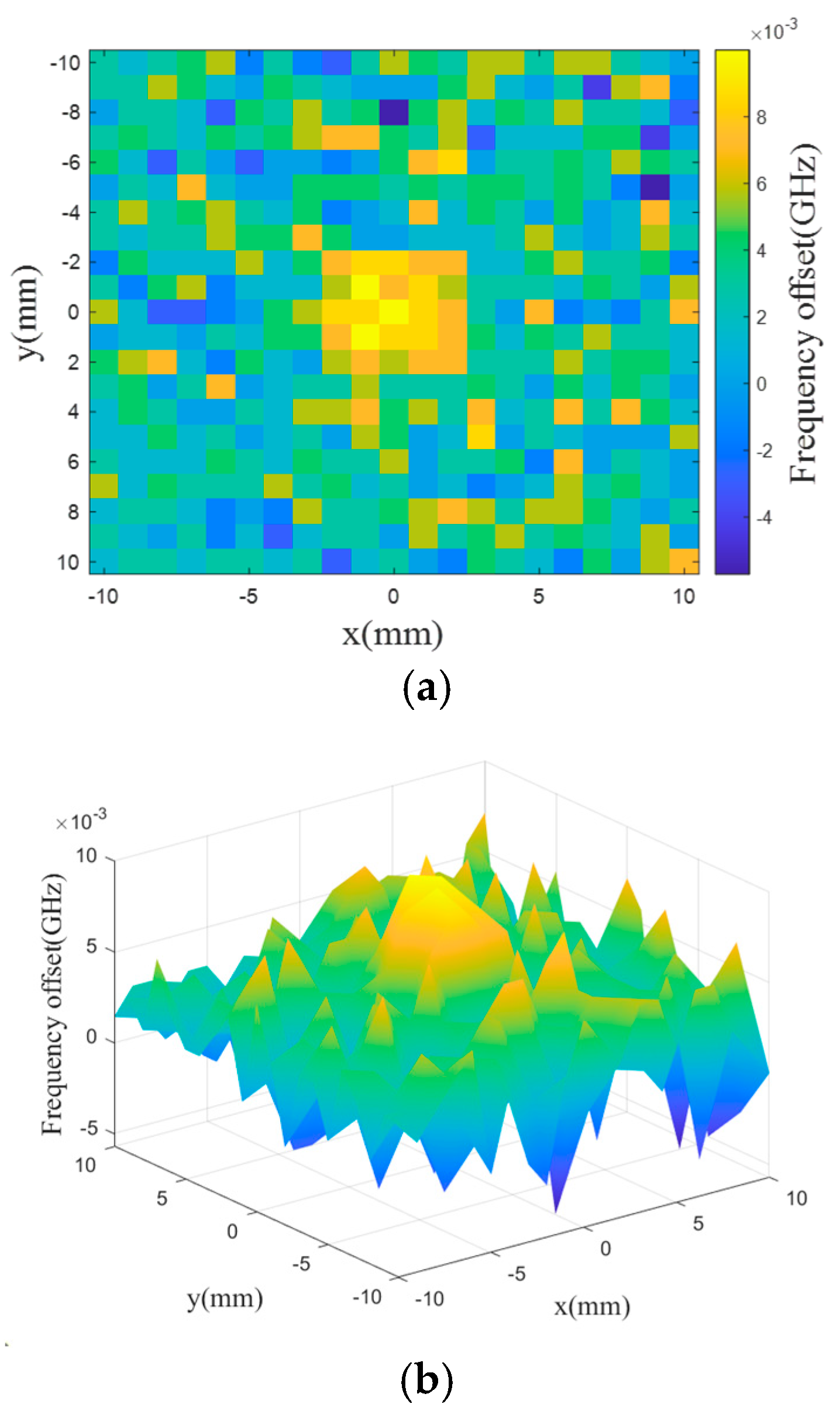
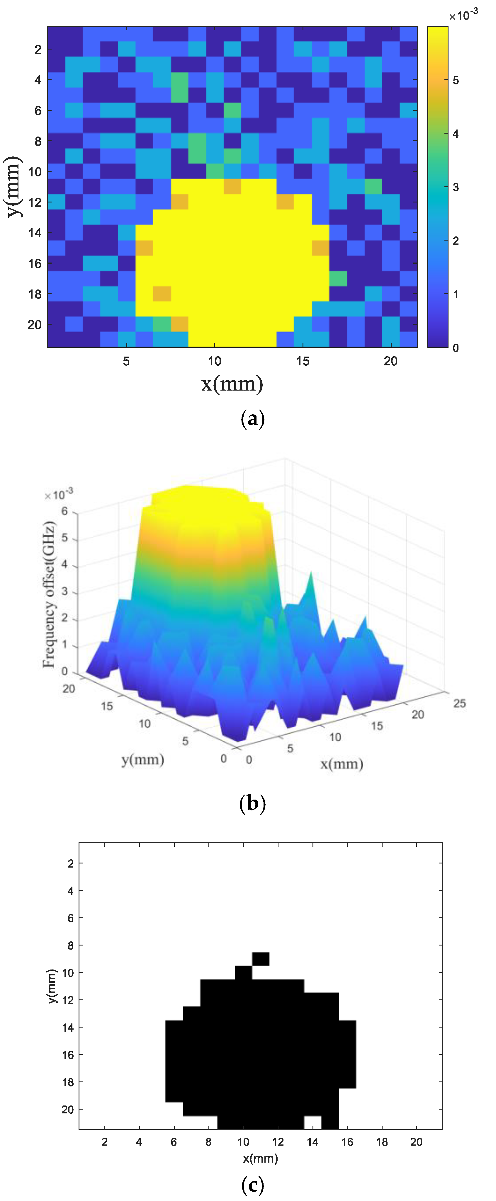
4.2. Internal Defects in the MUT

This paper constructed a carbon fiber composite material model of 80 mm × 80 mm with a thickness of 1.9 mm. The thickness of the carbon fiber layer of the composite material is 0.5 mm, and the thickness of the epoxy resin layer is 0.1 mm. The internal bubble defect is located in the epoxy resin layer. The bubble defect area is 5 mm × 5 mm × 0.05 mm, and the depth is 0.625 mm. The lifting distance from the resonant sensor to the composite material is 0.7 mm.

When the sensor scans the tested composite material, it covers an area of 20 mm × 20 mm, with a step size of 1 mm, and constructs a 441-pixel image in a two-dimensional scanning mode. Figure 9a,b show the top and side views of the tested composite materials. The scanning process and distribution of bubble defects are shown in Figure 10. For each scan position, the frequency is scanned in the frequency range 0.5 GHz to 1.0 GHz in 2 MHz increments. The scanned results are shown in Figure 11. Figure 11 shows an example of the amplitude-frequency plot of the $S_{21}$ parameter recorded at each scanning position, indicating that when the CSRR is close to the defect, an obvious frequency shift occurs.

Figure 9. (a) Defect top view; (b) Defect side view.

Figure 10. Scanning process and distribution of bubble defects.

Figure 11. $S_{21}$ parameter frequency-amplitude plot of 441 scan points near internal bubble defects.

The results of the scattering matrix are imported into the MATLAB environment for post-processing, and the simulation results are shown in Figure 12. The yellow rectangular area in Figure 12a shows the defective area, and the blue and green backgrounds correspond to the rest of the scanned area. The $S_{21}$ resonant frequency shift at the center of the internal bubble defect area is increased to 10 MHz. However, when the sensor moves away from the defect area, the $S_{21}$ resonant frequency offset starts to decrease.

Figure 12. (a) $S_{21}$ resonant frequency offset size at each scan position; (b) 3D plot of $S_{21}$ resonant frequency shift at each scan position.

The bubble defect reconstruction image of the tested composite material is shown in Figure 13. Black represents the defective area and white represents the defect-free area. The reconstructed image is based on the data obtained by the metamaterial sensor. PCA is used for data dimensionality reduction. Considering the binary classification situation, SVM is used to implement the model. The size of the reconstructed bubble defect is basically consistent with the size of the simulation setting. At the same time, due to the use of binary images, the imaging of the bubble defect can be more prominent. The trained model can better characterize bubble defects in carbon fiber composite materials.

Figure 13. Reconstructed image of internal bubble defects.

Similarly, for the detection of internal fiber breakage defects in CFRP, the fiber breakage defect area is 5 mm × 10 mm × 0.05 mm with a depth of 1 mm. The fiber breakage defect reconstruction image of the tested composite material is shown in Figure 14.

Figure 14. Reconstructed image of internal fiber breakage defects.

Based on the above, simulation analysis was conducted on two common defects in CFRP, namely internal bubbles and fiber breakage, and the results showed that both can achieve good defect reconstruction and localization. This method can also be extended to the detection of other types of defects.

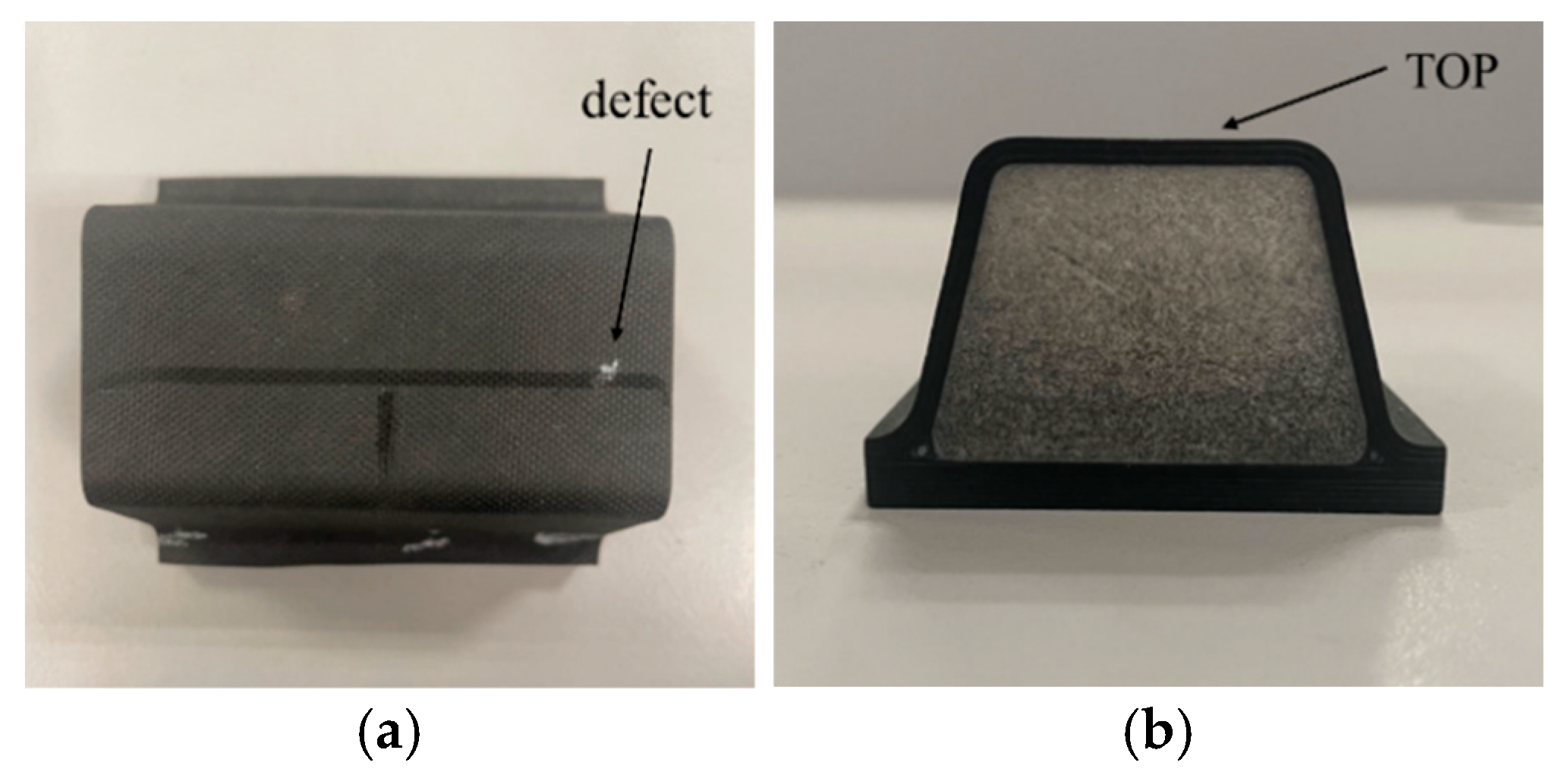
4.3. Experimental Results and Analysis of Aircraft Skin

This paper uses aircraft skin composite material as the MUT, which is also a kind of carbon fiber composite material, and its structure is shown in Figure 15. Figure 15 shows the top view and cross-sectional view of the material, with white dots indicating the location of defects. The length of this material is 6.7 cm, and the width of the top is 3 cm. The defect size is 1 cm.

Figure 15. Aircraft skin. (a) Top view; (b) Cross section diagram.

The experimental platform includes a network analyzer, a resonance sensor, and the tested material. The experimental platform is shown in Figure 16. In the experiment, the metamaterial sensor was placed on the top of the material being tested, and a lifting distance was maintained between the sensor and the top plane of the material being tested. A sensor is used to perform a two-dimensional planar scan of the area near the defect on top of the material being tested.

Figure 16. Testing experimental platform.

For each scanning position, the frequency is scanned in the frequency range from 0.364 GHz to 1.220 GHz, and the scanning results are shown in Figure 17. The experiment uses a vector network analyzer (VNA) to obtain frequency sweep data, and also imports the original data obtained from the VNA into the Matlab environment for processing. The simulation results are shown in Figure 18. The $S_{21}$ resonant frequency shift in the defective area is increased to 6 MHz. The three-dimensional stereoscopic image constructed in Figure 18b can more intuitively show that the $S_{21}$ resonant frequency shift at the defective position increases, while the $S_{21}$ resonant frequency shift at the defect-free position is small or almost no shift.

Figure 17. Frequency amplitude plot of $S_{21}$ parameter for all scanning positions.

Figure 18. (a) $S_{21}$ resonant frequency offset size at each scan position; (b) 3D plot of $S_{21}$ resonant frequency shift at each scan position; (c) Reconstructed images of aircraft skin composite defects.

The reconstruction result of the defect was measured as shown in Figure 18c. The size of the reconstructed defect is basically consistent with the size of the actual object, and a binary image is used, so the imaging of the defect can be more prominent. There are also some redundant points on the black image boundary. According to the analysis, the paper conducted simulation training on two typical defects, namely bubbles and fiber breakage. Due to the diverse types of process defects, there may be a mismatch between the classification model and the actual product during actual testing. But as the data sets for training the model increases, the measured results will become more accurate.

5. Conclusions

This paper constructs simulation models of carbon fiber composite materials and metamaterial sensors, uses metamaterial sensors to scan defects near the tested material defects, and uses defect recognition and localization technology based on PCA and SVM to process the original scanning data to obtain reconstructed binary images of defects, achieving defect recognition and localization. The experimental results indicate that the defect recognition and localization technology based on principal component analysis and support vector machine used in this article can effectively characterize defects. However, industrial grade CFRP testing poses certain challenges, and the specific challenges and solutions are as follows:

(1)

The use of point by point scanning has the problem of low efficiency. An array sensor structure can be used.

(2)

The types of data sets constructed are limited, and there are many types of actual process defects, which may result in a mismatch between the classifier and the actual situation. By continuously conducting simulation experiments and increasing the simulation data sets, the accuracy of defect reconstruction and localization can be further improved.

(3)

The sensor adopts a rigid structure, which poses adaptability issues for detecting complex structures in industry. Flexible materials can be used to design sensors.

References

- Wang, T.; Wu, D.; Chen, W.; Yang, J. Detection of delamination defects inside carbon fiber reinforced plastic laminates by measuring eddy-current loss. Compos. Struct. 2021, 268, 114012. [Google Scholar] [CrossRef]
- Kharkovsky, S.; Zoughi, R. Microwave and millimeter wave nondestructive testing and evaluation—Overview and recent advances. IEEE Instrum. Meas. Mag. 2017, 10, 26–38. [Google Scholar] [CrossRef]
- Naqiuddin, M.S.M.; Leong, M.S.; Hee, L.M. Ultrasonic signal processing techniques for Pipeline: A review. MATEC Web Conf. 2019, 255, 06006. [Google Scholar] [CrossRef]
- Sambath, S.; Nagaraj, P.; Selvakumar, N. Automatic defect classification in ultrasonic NDT using artificial intelligence. J. Nondestruct. Eval. 2011, 30, 20–28. [Google Scholar] [CrossRef]
- Tipones, R.D.; Cruz, J.C.D. Design and development of a material impact tester using neural network for concrete ratio classification. In Proceedings of the IEEE 13th International Colloquium on Signal Processing & its Applications (CSPA), Penang, Malaysia, 10–12 March 2017; pp. 106–111. [Google Scholar]
- Ali, A.; Hu, B.; Ramahi, O. Intelligent Detection of Cracks in Metallic Surfaces Using a Waveguide Sensor Loaded with Metamaterial Elements. Sensors 2015, 15, 11402–11416. [Google Scholar] [CrossRef] [PubMed]
- Ali, A.; Albasir, A.; Ramahi, O.M. Microwave sensor for imaging corrosion under coatings utilizing pattern recognition. In Proceedings of the IEEE International Symposium on Antennas & Propagation, Fajardo, PR, USA, 26 June–1 July 2016; pp. 951–952. [Google Scholar]
- Moomen, A.; Ali, A.; Ramahi, O. Reducing Sweeping Frequencies in Microwave NDT Employing Machine Learning Feature Selection. Sensors 2016, 16, 559. [Google Scholar] [CrossRef] [PubMed]
- Kotriwar, Y.D.; Elshafiey, O.; Peng, L.; Li, Z.; Srinivasan, V.; Davis, E.; Deng, Y. Gradient feature-based method for defect detection of carbon fiber reinforced polymer materials. In Proceedings of the IEEE International Conference on Prognostics and Health Management (ICPHM), Montreal, QC, Canada, 5–7 June 2023; pp. 246–252. [Google Scholar]
- Liu, Z.; Roy, M.; Prasad, D.K.; Agarwal, K. Physics-guided loss functions improve deep learning performance in inverse scattering. IEEE Trans. Comput. Imaging 2022, 8, 236–245. [Google Scholar] [CrossRef]
- Holloway, C.L.; Sarto, M.S.; Johansson, M. Analyzing carbonffber composite materials with equivalent-layer models. IEEE Trans. Electromagn. Compat. 2005, 47, 833–844. [Google Scholar] [CrossRef]
- Jing, Z.; Cai, G.; Yu, X.; Wang, B. Ultrasonic detection and evaluation of delamination defects in carbon ffber composites based on ffnite element simulation. Compos. Struct. 2024, 353, 118749. [Google Scholar] [CrossRef]
- Cheng, J.; Wang, Y.Z.B.; Liu, M.; Xu, D.; Qiu, J.; Takagi, T. Noncontact visualization of multiscale defects in CFRP composites using eddy current testing with T-R probe. NDT E Int. 2024, 145, 103138. [Google Scholar] [CrossRef]
- Huang, J.; Wei, Q.; Zhuo, L.; Zhu, J.; Li, C.; Wang, Z. Detection and quantiffcation of artiffcial delaminations in CFRP composites using ultrasonic thermography. Infrared Phys. Technol. 2023, 130, 104579. [Google Scholar] [CrossRef]
Disclaimer/Publisher’s Note: The statements, opinions and data contained in all publications are solely those of the individual author(s) and contributor(s) and not of MDPI and/or the editor(s). MDPI and/or the editor(s) disclaim responsibility for any injury to people or property resulting from any ideas, methods, instructions or products referred to in the content. |
© 2024 by the authors. Licensee MDPI, Basel, Switzerland. This article is an open access article distributed under the terms and conditions of the Creative Commons Attribution (CC BY) license (https://creativecommons.org/licenses/by/4.0/).