Dynamic Evaluation of Adaptive Product Design Concepts Using m-Polar Linguistic Z-Numbers

Abstract

Adaptive design focuses on creating flexible products that meet evolving demands and enhance sustainability. However, evaluating adaptive design concepts poses significant challenges due to the dynamic nature of product features over time and the inherent uncertainty in decision-makers’ (DMs’) evaluations. Most traditional frameworks rely on static models that fail to capture the temporal evolution of attributes and often overlook decision-makers’ (DMs’) confidence levels, resulting in incomplete or unreliable evaluations. To bridge these gaps, we propose the m-polar linguistic Z-number (mLZN) to address these issues. This framework uses the dynamic representation capabilities of m-polar fuzzy sets (mFSs) and the symmetrical structure of linguistic Z-numbers (LZNs), which effectively integrate linguistic evaluations with corresponding confidence levels, providing a balanced and robust approach to handling uncertainty. This approach models design characteristics across multiple periods while accounting for DMs’ confidence levels. Based on this framework, we develop mLZN weighted and geometric aggregation operators, computation rules, and ranking methods to support dynamic multi-attribute group decision-making (MAGDM). The proposed framework’s effectiveness is demonstrated through a case study on adaptive furniture design for children, which showcases its ability to dynamically evaluate key attributes, including safety, ease of use, fun, and comfort. Furthermore, we validate its robustness and feasibility through comprehensive sensitivity and comparative analyses.

1. Introduction

Adaptive design is a product development approach to create flexible and modular products that respond to evolving customer demands while enhancing sustainability and reducing environmental impact [1,2,3]. Unlike traditional design methods, which often lock products into fixed functionalities and operating conditions [4], adaptive design emphasizes the ability to modify or upgrade products during their operational phase [5]. This flexibility extends product lifecycles, reduces waste, enhances cost efficiency, and provides a competitive edge in rapidly changing markets [6]. However, evaluating the concept of adaptive design presents unique challenges, as it must consider the dynamic nature of product attributes, constantly changing environmental conditions, and user preferences and uncertainties at different stages [7].

The MAGDM method has been widely adopted in the literature related to design evaluation to address challenges related to product design requirement analysis and solution selection [8,9]. These methods offer structured frameworks to compare and prioritize design alternatives based on multiple attributes, enabling DMs to integrate diverse perspectives and balance conflicting objectives [10,11]. In addition, the MAGDM method, which integrates fuzzy sets [12,13] and linguistic terms, effectively solves the uncertainty and inaccuracy in design concept evaluation [14,15]. Adaptiveness refers to the ability of a system or product to adjust dynamically to varying conditions or requirements over time. It is an inherently fuzzy concept, as it involves continuous changes and dependencies that are difficult to quantify precisely. For instance, in adaptive design, furniture designed for children’s growth must adjust attributes such as size, safety features, and materials dynamically as the child ages. Traditional methods often struggle to model how these attributes evolve across different stages of a product’s lifecycle, resulting in incomplete or static evaluations. Moreover, these methods frequently overlook DMs’ confidence levels in their assessments, which can lead to less reliable or inconsistent decisions in scenarios characterized by high uncertainty or conflicting judgments.

Existing methods for dynamic MAGDM face challenges in capturing the temporal evolution of attributes and integrating DMs’ confidence levels [9,16,17], often relying on static models that lead to incomplete or unreliable evaluations. To address these gaps, we propose the mLZN framework, which combines the dynamic modeling capabilities of mFS [18] and LZN [19]. mFSs are advanced mathematical models that allow for the representation of multiple evaluations for the same attribute under different conditions or periods through distinct “poles” [20,21]. Each pole corresponds to a specific temporal state or scenario, enabling dynamic modeling of attribute performance over time. For example, in evaluating adaptive furniture design, mFSs can represent variations in size, safety, and functionality across different growth stages of a child, providing a comprehensive view of the attribute’s evolution. On the other hand, LZNs enhance traditional fuzzy logic by incorporating both a linguistic evaluation of an attribute (e.g., “high safety” or “moderate comfort”) and a linguistic representation of the confidence level in that evaluation (e.g., “very confident” or “uncertain”) [19,22,23]. This dual-component structure addresses the uncertainty and variability inherent in decision-making by offering a clear and intuitive assessment while capturing the reliability of the evaluations. By combining these two techniques, the mLZN framework enables a dynamic and comprehensive evaluation of adaptive design concepts. The temporal modeling capabilities of mFSs are complemented by the uncertainty-handling and confidence-representation strengths of LZNs, making the method particularly suitable for dynamic, multi-attribute decision problems where both the evolution of attributes over time and the reliability of evaluations must be considered. This integration is expected to provide a robust solution to the limitations of traditional MAGDM methods, ensuring reliable and actionable decision-making in the context of adaptive design.

We summarize our work contributions as follows:

• We introduce the mLZN, a novel structure for modeling multidimensional, dynamic, and multi-attribute decision-making scenarios. By integrating the dynamic representation of mFSs with the uncertainty-handling capabilities of LZNs, mLZN provides a comprehensive framework to address temporal variability and linguistic uncertainty in decision-making processes.
• We develop the operational rules for mLZNs, including score function and ranking rules. Building on these foundations, we propose four aggregation operators: mLZN weighted average (mLZNWA), mLZN ordered weighted average (mLZNOWA), mLZN weighted geometric (mLZNWG), and mLZN ordered weighted geometric (mLZNOWG) operators. We develop these operators to dynamically aggregate uncertain linguistic information, and we analyze their critical properties, such as monotonicity and commutativity, to demonstrate their effectiveness.
• We validate the proposed mLZN-based approach through a case study on adaptive children’s furniture design. The case study showcases mLZN’s ability to handle dynamic linguistic decision-making by capturing temporal changes in attributes and integrating expert evaluations with confidence levels. A comparative analysis further demonstrates the superior performance of mLZN in managing dynamic, language-based decision problems, highlighting its practical value and robustness.
• We have arranged the remaining parts of this work as follows: Section 2 introduces our work’s background, including the MAGDM method’s research in product design evaluation, mFSs, and LZNs. In this section, we summarize the research gap and our motivation. Section 3 describes the basic theory of mLZNs, the proposed aggregation operator, and the dynamic mLZN-based MAGDM method. Section 4 showcases the implementation process of our mLZN-based MAGDM method through the design case of children’s adaptive furniture. Section 5 conducts a sensitivity analysis and comparative analysis of the methods. Finally, we summarize our work and limitations in Section 6.

2. Background

2.1. Research on MAGDM for Design Evaluation

The evaluation of adaptive product concept designs has received limited attention in existing research. However, it is an integral part of design evaluation studies. To situate our study in this context, we summarize the current advancements in applying MAGDM methods for design evaluation. Fuzzy MAGDM methods [8,9,14,15] are widely utilized in conceptual design evaluation because they can address the uncertainty and fuzziness inherent in decision-making processes. These methods enhance decision-making by integrating the opinions and weights of different DMs, using fuzzy logic to effectively capture the relative strengths and weaknesses of each conceptual design alternative.

Among these methods, Tiwari et al. [16] introduced an improved VIKOR (Vlsekriterijumska Optimizacija I Kompromisno Resenje) method based on rough sets to evaluate product design concepts. This approach focuses on determining the optimal design concept that aligns with the design team’s constraints and maximizes customer preferences without explicitly considering the cost–benefit characteristics of design criteria. Zhu et al. [24] proposed a novel hierarchical analysis process (AHP) based on rough numbers to assign weights to evaluation criteria. They use rough numbers to evaluate and compare design concept alternatives, enhancing the VIKOR method’s ability to handle uncertainty in DM groups. Similarly, Cui et al. [8] developed a conceptual design evaluation framework incorporating multi-granularity heterogeneous evaluation semantics and uncertain beliefs. They utilized cloud model distributions to create an advantage matrix and selected the best solution through the VIKOR method.

In the study of evaluating conceptual designs using Z-numbers [25], Liu et al. [26] further advanced this area by proposing a selection method incorporating decision-maker confidence levels through AHP and the technique for order preference by similarity to the ideal solution (TOPSIS). In addition, Liu et al. [27] proposed an evaluation method for human–machine interface conceptual design using spherical fuzzy AHP combined with axiomatic design principles. This approach effectively integrates design standards and DM’s preferences. Regarding the consideration of decision-maker confidence, Aydoğan et al. [9] introduced a Z-number-based axiomatic design evaluation method for conceptual design schemes. Additionally, Jing et al. [17] developed a conceptual decision model using interval-valued intuitionistic fuzzy sets, which integrates evaluation data for similar preferences and determines the optimal solution through weighted aggregation operators based on customer preference distributions. Recently, Jing et al. [28] proposed a patent-based conceptual design evaluation approach that addresses incomplete semantics and subjective scheme beliefs by integrating historical patent data, strong association rules, and a fuzzy evidence theory model. The approach accounts for non-compensatory interactions between decision-makers and criteria to enhance the objectivity and reliability of selecting optimal conceptual schemes.

These studies collectively demonstrate the diverse applications of MAGDM methods in design evaluation, highlighting their ability to accommodate complexity, uncertainty, and varied customer requirements in selecting optimal product design concepts.

2.2. Research on mFSs

Recent research on mFSs has expanded their applications and theoretical advancements across various domains [29,30,31,32], showcasing their capability to handle multidimensional uncertainty and complex decision-making scenarios. Researchers have explored mPFS to model multi-polar information, addressing challenges such as decision support systems, linguistic analysis, graph theory, and MAGDM. These works highlight the usability of mPFS in integrating fuzzy logic with multi-polar frameworks to solve real-world problems.

Rahman et al. [30] introduced m-polar fuzzy Aczel–Alsina aggregation operators, applying them to site selection problems for desalination and wind power plants. They demonstrated their effectiveness compared to other T-norm-based methods. Sivakumar et al. [31] utilized m-polar neutrosophic sets to analyze mood changes and depression on social media, combining linguistic and machine learning techniques for Arabic text processing. Akram et al. [32] extended the ELECTRE-III method with two-tuple linguistic m-polar fuzzy data for MAGDM. They validated it through anti-aircraft missile system selection. Similarly, another study by Akram et al. [33] applied m-polar fuzzy graphs to connectivity analysis in product manufacturing, introducing metrics to evaluate network performance. Bera et al. [34] incorporated m-polar interval-valued fuzzy graphs into facility location problems, introducing double domination to manage uncertainty. Ali et al. [29] developed interval-valued m-polar fuzzy soft expert sets, applying them to optimize prosthesis designs in a group decision-making context. Additionally, Akram et al. [35] proposed an m-polar fuzzy N-soft PROMETHEE approach for alternative evaluation in digitization projects, emphasizing its ability to manage complex, multi-polar uncertainty. Alshayea and Alsager [36] defined m-polar Q-hesitant anti-fuzzy sets, extending fuzzy logic to mathematical algebras. Kausar et al. [37] employed cubic mFSs with Schweizer–Sklar aggregation operators to enhance algorithm selection in information retrieval systems, addressing considerable dataset challenges effectively.

This research emphasizes the rapid development and diverse applicability of the mFS theory. By combining multipole information with fuzzy set techniques, these works have made significant contributions to solving complex problems in decision-making and network analysis, demonstrating the potential of mPFS in future research and applications, particularly in dynamic MAGDM.

2.3. Research on LZNs

Recent LZN research has significantly expanded its theoretical foundations and applications in decision-making under uncertainty. As a powerful extension of Zadeh’s Z-numbers [25], LZNs [19] combine linguistic terms with credibility levels to address the fuzziness and reliability of decision-making information. These studies have explored various novel frameworks and methodologies, showcasing the adaptability and effectiveness of LZN-based MAGDM problems, particularly in complex and uncertain environments.

Jia et al. [38] introduced a polar coordinate system for LZNs, simplifying computations and enhancing their applicability in MAGDM. They proposed the Z-polar coordinate vector synthesis power-weighted operator for aggregating multi-criteria information. Li [39] proposed a dual perspective method using LZNs for driving behavior risk evaluation, effectively capturing uncertainties and divergences in decision-making through an α-truncation set and utility functions. Chen et al. [40] integrated LZNs with IF-THEN rules based on a rectangular coordinate system to address reasoning in MAGDM, demonstrating the method’s effectiveness in epidemic-level assessment and network security. Wang et al. [41] developed a TODIM-based method for MAGDM with LZNs, incorporating the Choquet integral to manage interactivity between criteria. Chai et al. [42] proposed a preference relation approach using LZNs to assess digital transformation in SMEs, emphasizing consistency and enhanced MAGDM models. Tao et al. [43] introduced the concept of LZN fuzzy soft sets, combining fuzzy logic and soft sets to solve MAGDM problems with extended TOPSIS models. Liu et al. [44] introduced linguistic q-rung orthopair fuzzy Z-numbers, combining multiple fuzzy theories to enhance the reliability of decision-making in airline aircraft selection. Fan et al. [45] applied interval-valued LZNs to improve risk prioritization in FMEA, demonstrating their potential in quality management.

The above research indicates the advantages of LZNs in addressing uncertainty and ambiguity in decision-making. These operational frameworks, aggregation operators, and application domains demonstrate the potential of extending LZNs to multidimensional and dynamic decision-making environments.

2.4. Research Gaps and Motivations

• Despite the growing interest in MAGDM methods, existing approaches face notable limitations when addressing dynamic decision-making scenarios with linguistic uncertainty and decision-maker confidence levels. Traditional MAGDM frameworks often fail to model the temporal variability of attributes, which is essential for evaluating evolving alternatives, such as adaptive product designs [16,17,26]. Furthermore, while LZNs have effectively captured uncertainty and reliability, their applications have focused mainly on static decision problems and have not been extended to multidimensional, dynamic contexts. Additionally, current methods often overlook the integration of linguistic evaluations with confidence measures in multi-polar decision-making environments, leaving a significant gap in handling complex, time-sensitive evaluations.
• Our research is motivated by developing a comprehensive framework combining mFSs and LZNs’ strengths. The unique capability of mFSs to model dynamic, multi-polar information provides a robust foundation for addressing temporal variability. At the same time, LZNs enable the incorporation of DM confidence levels into the evaluation process. By integrating these two powerful concepts, we aim to create a novel decision-making framework that bridges the limitations of existing methods, providing a comprehensive approach to dynamic MAGDM problems. This motivation is further driven by the increasing demand for practical decision-making tools in adaptive product design evaluations, where attributes change over time, and uncertainty is inherently present.

3. Method

3.1. Preliminaries

This section reviews some basic definitions necessary for our proposed mLZN.

Definition 1 ([46,47,48,49]).

Let $S=\left\{s_0,s_1,s_2,\dots ,s_{2t}\right\}$ be a discrete linguistic term set (LTS) with a finite odd cardinality. $s_l\in S$ is called a linguistic term (LT) representing a possible value for a linguistic variable. For an LTS $S=\left\{s_0,s_1,s_2,\dots ,s_{2t}\right\}$, the following properties must be satisfied:

1. 

The set S is ordered: $s_a>s_b$ if and only if $a>b$.

2. 

There is a negation operator: $neg\left(s_a\right)=s_{2t-a}$.

Continuous LTS (CLTS) is an extension of discrete LTS that describes a more extensive range of linguistic variables, which can be defined as ${\overline{S}}_{\left[0,l\right]}=\left\{s_0\le s_{\alpha }\le s_l,\alpha \in \left[0,l\right]\right\}$. CLTS can express linguistic variables between discrete LTs in virtual terms form. For example, $s_{1.5}$ between $s_1$ and $s_2$.

Definition 2 ([48]).

Let $S=\left\{s_0,s_1,s_2,\dots ,s_{2t}\right\}$ be a LTS and ${\theta }_l\in \left[0,1\right]\left(l=0,1,\dots ,2t\right)$. Then, the linguistic scale function (LSF) is a mapping $\mathfrak{F}$ from $s_l\in S$ to ${\theta }_l$, which is defined as

$$\mathfrak{F}:s_l\to {\theta }_l$$

(1)

where $0\le {\theta }_0\le {\theta }_1\le$…$\le {\theta }_{2t}\le 1$. In other words, LSF is a monotone-increasing function. Some commonly used LSFs are as follows [19,48,50]:

$${\mathfrak{F}}_1\left(s_l\right)={\theta }_l={\displaystyle \frac{l}{2t}} \left(l=0,1,2,\dots ,t\right)$$

(2)

$${\mathfrak{F}}_2\left(s_l\right)={\theta }_l=\left\{\begin{array}{c}{\displaystyle \frac{{\alpha }^t-{\alpha }^{t-l}}{2{\alpha }^t-2}} \left(l=0,1,2,\dots ,t\right)\\ {\displaystyle \frac{{\alpha }^t+{\alpha }^{l-t}-2}{2{\alpha }^t-2}} \left(l=t+1,t+2,\dots ,2t\right)\end{array}\right.$$

(3)

where $\alpha$ can be obtained through experiments or subjective methods, usually $\alpha =1.37$. In ${\mathfrak{F}}_2$, the absolute deviation between adjacent LTs increases as the LTS expands from the middle to both ends [51].

$${\mathfrak{F}}_3\left(s_l\right)={\theta }_l=\left\{\begin{array}{c}{\displaystyle \frac{t^{\alpha }-{\left(t-l\right)}^{\alpha }}{2t^{\alpha }}} \left(l=0,1,2,\dots ,t\right)\\ {\displaystyle \frac{t^{\beta }-{\left(l-t\right)}^{\beta }}{2t^{\beta }}} \left(l=t+1,t+2,\dots ,2t\right)\end{array}\right.$$

(4)

where $\alpha ,\beta \in \left[0,1\right]$. In ${\mathfrak{F}}_3$, as the LTS expands from the middle to both ends, the absolute deviation between adjacent LTs will decrease [51]. In this work, we take $\alpha =\beta =0.88$ based on the prospect theory [50].

Definition 3 ([19]).

Let X be a universe of discourse and $S_1=\left\{s_0,s_1,s_2,\dots ,s_{2t}\right\}$ and $S_2=\left\{{s^{\prime }}_0,{s^{\prime }}_1,{s^{\prime }}_2,\dots ,{s^{\prime }}_{2k}\right\}$ be two finite and totally ordered discrete LTSs, where l and k are positive integers. Then, an LZN set $\mathcal{Z}$ in X is defined in the following form:

$$\mathcal{Z}=\left\{\left(x,{\mathcal{A}}_{\mathcal{f}\left(x\right)},{\mathcal{B}}_{\mathcal{g}\left(x\right)}\right)\left|x\in X\right.\right\}$$

(5)

where ${\mathcal{A}}_{\mathcal{f}\left(x\right)}$ and ${\mathcal{B}}_{\mathcal{g}\left(x\right)}$ are represented by two LTSs, $S_1$ and $S_2$. ${\mathcal{A}}_{\mathcal{f}\left(x\right)}$ is a linguistic fuzzy constraint on the values allowed for uncertain variables $x$, and ${\mathcal{B}}_{\mathcal{g}\left(x\right)}$ is the linguistic reliability measure of ${\mathcal{A}}_{\mathcal{f}\left(x\right)}$. For convenience, ${\mathcal{z}}_{\alpha }=\left({\mathcal{A}}_{{\mathcal{f}}_{\alpha }},{\mathcal{B}}_{{\mathcal{g}}_{\alpha }}\right)$ is called an LZN, where ${\mathcal{A}}_{{\mathcal{f}}_{\alpha }}\in S_1$ and ${\mathcal{B}}_{{\mathcal{g}}_{\alpha }}\in S_2$ are two LTs.

Definition 4 ([19]).

The score function of LZN ${\mathcal{z}}_{\alpha }=\left({\mathcal{A}}_{{\mathcal{f}}_{\alpha }},{\mathcal{B}}_{{\mathcal{g}}_{\alpha }}\right)$ is defined as

$$S\left({\mathcal{z}}_{\alpha }\right)={\mathfrak{F}}_p\left({\mathcal{A}}_{{\mathcal{f}}_{\alpha }}\right)\times {\mathfrak{F}}_q\left({\mathcal{B}}_{{\mathcal{g}}_{\alpha }}\right)$$

(6)

where $S\left({\mathcal{z}}_{\alpha }\right)\in \left[0,1\right]$ and $\mathfrak{F}$ is an LSF. In general, p $\ne$ q.

Definition 5 ([19]).

The accuracy function of LZN ${\mathcal{z}}_{\alpha }=\left({\mathcal{A}}_{{\mathcal{f}}_{\alpha }},{\mathcal{B}}_{{\mathcal{g}}_{\alpha }}\right)$ is defined as

$$A\left({\mathcal{z}}_{\alpha }\right)={\mathfrak{F}}_p\left({\mathcal{A}}_{{\mathcal{f}}_{\alpha }}\right)\times \left(1-{\mathfrak{F}}_q\left({\mathcal{B}}_{{\mathcal{g}}_{\alpha }}\right)\right)$$

(7)

where $A\left(\mathfrak{s}\right)\in \left[0,1\right]$ and $\mathfrak{F}$ is an LSF. In general, p $\ne$ q.

Definition 6 ([19]).

Let ${\mathcal{z}}_{\alpha }=\left({\mathcal{A}}_{{\mathcal{f}}_{\alpha }},{\mathcal{B}}_{{\mathcal{g}}_{\alpha }}\right)$ and ${\mathcal{z}}_{\beta }=\left({\mathcal{A}}_{{\mathcal{f}}_{\beta }},{\mathcal{B}}_{{\mathcal{g}}_{\beta }}\right)$ be any two LZNs; then, an ordered relation between these two LZNs is established as follows:

1. 

If $S\left({\mathcal{z}}_{\alpha }\right)<S\left({\mathcal{z}}_{\beta }\right)$, then ${\mathcal{z}}_{\alpha }<{\mathcal{z}}_{\beta }$;

2. 

If $S\left({\mathcal{z}}_{\alpha }\right)>S\left({\mathcal{z}}_{\beta }\right)$, then ${\mathcal{z}}_{\alpha }>{\mathcal{z}}_{\beta }$;

3. 

If $S\left({\mathcal{z}}_{\alpha }\right)=S\left({\mathcal{z}}_{\beta }\right)$, then

• If $A\left({\mathcal{z}}_{\alpha }\right)<A\left({\mathcal{z}}_{\beta }\right)$, then ${\mathcal{z}}_{\alpha }<{\mathcal{z}}_{\beta }$;
• If $A\left({\mathcal{z}}_{\alpha }\right)>A\left({\mathcal{z}}_{\beta }\right)$, then ${\mathcal{z}}_{\alpha }>{\mathcal{z}}_{\beta }$;
• If $A\left({\mathcal{z}}_{\alpha }\right)=A\left({\mathcal{z}}_{\beta }\right)$, then ${\mathcal{z}}_{\alpha }={\mathcal{z}}_{\beta }$.

Definition 7 ([18]).

An mFS $\mathfrak{C}$ on a nonempty set X is defined as a mapping $\mathfrak{C}:X\to {\left[0,1\right]}^m$ and the membership degree for every element $x\in X$ is denoted as

$$\mathfrak{C}=\left(p_1\circ \mathfrak{C}\left(x\right),p_2\circ \mathfrak{C}\left(x\right),\dots ,p_m\circ \mathfrak{C}\left(x\right)\right)$$

(8)

where $p_i\circ \mathfrak{C}:{\left[0,1\right]}^m\to \left[0,1\right]$ is the i-th projection mapping, extracting the i-th membership value from the vector. The set ${\left[0,1\right]}^m$, representing the m-th Cartesian power of the unit interval $\left[0,1\right]$, is equipped with a natural partial order such that for any $x,y\in {\left[0,1\right]}^m,$ $x\le y$ if and only if $p_i\left(x\right)\le p_i\left(y\right)$ for all i = 1, 2, …, m. The greatest element in ${\left[0,1\right]}^m$ is $\left(1,1,\dots ,1\right)$, and and the least element is $\left(0,0,\dots ,0\right)$.

According to Definition 7, we can observe that mFS structure allows for the mFS to model multidimensional membership values for elements, where each dimension corresponds to a specific attribute or perspective, extending the classical fuzzy set to effectively accommodate multi-polarity scenarios.

3.2. m-Polar Linguistic Z-Number

The concept of the mLZN integrates the multidimensional representation of membership functions from mFSs with the dual-component structure of LZNs. This new framework is designed to handle scenarios where uncertainty spans multiple dimensions, and linguistic descriptors and reliability measures characterize each dimension.

Definition 8.

Formally, an mLZN set is defined over a universe X, where each element $x\in X$ is associated with a linguistic descriptor ${\mathcal{A}}_{\mathcal{f}\left(x\right)}$ and a reliability measure ${\mathcal{B}}_{\mathcal{g}\left(x\right)}$ across m dimensions. Specifically, mLZN set can be expressed as

$$\Psi =\left\{\left(x,\left({\mathcal{A}}_{{\mathcal{f}}_1\left(x\right)},{\mathcal{B}}_{{\mathcal{g}}_1\left(x\right)}\right),\left({\mathcal{A}}_{{\mathcal{f}}_2\left(x\right)},{\mathcal{B}}_{{\mathcal{g}}_2\left(x\right)}\right),\dots ,\left({\mathcal{A}}_{{\mathcal{f}}_m\left(x\right)},{\mathcal{B}}_{{\mathcal{g}}_m\left(x\right)}\right)\right)\left|x\in X\right.\right\}$$

(9)

In Equation (9), ${\mathcal{A}}_{{\mathcal{f}}_i\left(x\right)}$ is an LT representing a fuzzy restriction in the i-th dimension, selected from a finite, totally ordered LTS $S_1$, and ${\mathcal{B}}_{{\mathcal{g}}_i\left(x\right)}$ is a LT representing the reliability of ${\mathcal{A}}_{{\mathcal{f}}_i\left(x\right)}$, selected from a finite, totally ordered LTS $S_2$. m represents the number of polarities (dimensions) considered, enabling the modeling of multiple independent yet interconnected perspectives. For convenience, we say ${\wp }_{\alpha }=\left(\left({\mathcal{A}}_{{\mathcal{f}}_{\alpha 1}},{\mathcal{B}}_{{\mathcal{g}}_{\alpha 1}}\right),\left({\mathcal{A}}_{{\mathcal{f}}_{\alpha 2}},{\mathcal{B}}_{{\mathcal{g}}_{\alpha 2}}\right),\dots ,\left({\mathcal{A}}_{{\mathcal{f}}_{\alpha m}},{\mathcal{B}}_{{\mathcal{g}}_{\alpha m}}\right)\right)$, an mLZN, where ${\mathcal{A}}_{{\mathcal{f}}_{\alpha i}}\in S_1$ and ${\mathcal{B}}_{{\mathcal{g}}_{\alpha i}}\in S_2$.

Because mFSs are used to handle fuzziness and uncertainty, overly strict partial sorting rules, such as comparing the membership degrees of each pole (Definition 7), may mask the essence of fuzzy sets. Therefore, we propose to use an approximate mLZNs ranking rule through score and accuracy functions to better adapt to the characteristics of fuzzy linguistic variables.

Definition 9.

The score function of mLZN ${\wp }_{\alpha }=\left(\left({\mathcal{A}}_{{\mathcal{f}}_{\alpha 1}},{\mathcal{B}}_{{\mathcal{g}}_{\alpha 1}}\right),\left({\mathcal{A}}_{{\mathcal{f}}_{\alpha 2}},{\mathcal{B}}_{{\mathcal{g}}_{\alpha 2}}\right),\dots ,\left({\mathcal{A}}_{{\mathcal{f}}_{\alpha m}},{\mathcal{B}}_{{\mathcal{g}}_{\alpha m}}\right)\right)$ is defined as

$$\mathbb{S}\left({\wp }_{\alpha }\right)={\displaystyle \frac{1}{m}}\left({\sum }_{i=1}^m{\mathfrak{F}}_p\left({\mathcal{A}}_{{\mathcal{f}}_{\alpha i}}\right){\mathfrak{F}}_q\left({\mathcal{B}}_{{\mathcal{g}}_{\alpha i}}\right)\right)$$

(10)

where $\mathbb{S}\left({\wp }_{\alpha }\right)\in \left[0,1\right]$ and $\mathfrak{F}$ is an LSF with p $\ne$ q.

Definition 10.

The accuracy function of mLZN ${\wp }_{\alpha }=\left(\left({\mathcal{A}}_{{\mathcal{f}}_{\alpha 1}},{\mathcal{B}}_{{\mathcal{g}}_{\alpha 1}}\right),\left({\mathcal{A}}_{{\mathcal{f}}_{\alpha 2}},{\mathcal{B}}_{{\mathcal{g}}_{\alpha 2}}\right),\dots ,\left({\mathcal{A}}_{{\mathcal{f}}_{\alpha m}},{\mathcal{B}}_{{\mathcal{g}}_{\alpha m}}\right)\right)$ is defined as

$$\mathbb{A}\left({\wp }_{\alpha }\right)={\displaystyle \frac{1}{m}}\left({\sum }_{i=1}^m{\mathfrak{F}}_p\left({\mathcal{A}}_{{\mathcal{f}}_{\alpha i}}\right)\left({1-\mathfrak{F}}_q\left({\mathcal{B}}_{{\mathcal{g}}_{\alpha i}}\right)\right)\right)$$

(11)

where $\mathbb{A}\left({\wp }_{\alpha }\right)\in \left[0,1\right]$ and $\mathfrak{F}$ is a LSF with p $\ne$ q.

Definition 11.

Let ${\wp }_{\alpha }=\left(\left({\mathcal{A}}_{{\mathcal{f}}_{\alpha 1}},{\mathcal{B}}_{{\mathcal{g}}_{\alpha 1}}\right),\left({\mathcal{A}}_{{\mathcal{f}}_{\alpha 2}},{\mathcal{B}}_{{\mathcal{g}}_{\alpha 2}}\right),\dots ,\left({\mathcal{A}}_{{\mathcal{f}}_{\alpha m}},{\mathcal{B}}_{{\mathcal{g}}_{\alpha m}}\right)\right)$ and ${\wp }_{\beta }=\left(\left({\mathcal{A}}_{{\mathcal{f}}_{\beta 1}},{\mathcal{B}}_{{\mathcal{g}}_{\beta 1}}\right),\left({\mathcal{A}}_{{\mathcal{f}}_{\beta 2}},{\mathcal{B}}_{{\mathcal{g}}_{\beta 2}}\right),\dots ,\left({\mathcal{A}}_{{\mathcal{f}}_{\beta m}},{\mathcal{B}}_{{\mathcal{g}}_{\beta m}}\right)\right)$ be any two mLZNs; then, an ordered relation between these two mLZNs is established as follows:

1. 

If $\mathbb{S}\left({\mathcal{z}}_{\alpha }\right)<\mathbb{S}\left({\mathcal{z}}_{\beta }\right)$, then ${\mathrm{\wp }}_{\alpha }\prec {\mathrm{\wp }}_{\beta }$ (${\mathcal{z}}_{\alpha }$ is inferior to ${\mathrm{\wp }}_{\beta }$);

2. 

If $\mathbb{S}\left({\mathcal{z}}_{\alpha }\right)>\mathbb{S}\left({\mathcal{z}}_{\beta }\right)$, then ${\wp }_{\alpha }\succ {\wp }_{\beta }$ (${\mathcal{z}}_{\alpha }$ is superior to ${\wp }_{\beta }$);

3. 

If $\mathbb{S}\left({\mathcal{z}}_{\alpha }\right)=\mathbb{S}\left({\mathcal{z}}_{\beta }\right)$, then,

• If $\mathbb{A}\left({\mathcal{z}}_{\alpha }\right)<\mathbb{A}\left({\mathcal{z}}_{\beta }\right)$, then ${\wp }_{\alpha }\prec {\wp }_{\beta }$ (${\mathcal{z}}_{\alpha }$ is inferior to ${\wp }_{\beta }$);
• If $\mathbb{A}\left({\mathcal{z}}_{\alpha }\right)>\mathbb{A}\left({\mathcal{z}}_{\beta }\right)$, then ${\wp }_{\alpha }\succ {\wp }_{\beta }$ (${\mathcal{z}}_{\alpha }$ is superior to ${\wp }_{\beta }$);
• If $\mathbb{A}\left({\mathcal{z}}_{\alpha }\right)=\mathbb{A}\left({\mathcal{z}}_{\beta }\right)$, then ${\wp }_{\alpha }\sim {\wp }_{\beta }$ (${\mathcal{z}}_{\alpha }$ is equivalent to ${\wp }_{\beta }$).

3.3. Operational Rules of mLZNs

Uncertainty information aggregation is significant in MAGDM, and mLZN is no exception [29,30,31,32]. In this section, we first propose operational rules for mLZNs. Next, we use these operational rules to develop weighted averaging and geometric aggregation operators.

Definition 12.

Assume that $\wp =\left(\left({\mathcal{A}}_{{\mathcal{f}}_1},{\mathcal{B}}_{{\mathcal{g}}_1}\right),\left({\mathcal{A}}_{{\mathcal{f}}_2},{\mathcal{B}}_{{\mathcal{g}}_2}\right),\dots ,\left({\mathcal{A}}_{{\mathcal{f}}_m},{\mathcal{B}}_{{\mathcal{g}}_m}\right)\right)$, ${\wp }_1=\left(\left({\mathcal{A}}_{{\mathcal{f}}_{11}},{\mathcal{B}}_{{\mathcal{g}}_{11}}\right),\left({\mathcal{A}}_{{\mathcal{f}}_{12}},{\mathcal{B}}_{{\mathcal{g}}_{12}}\right),\dots ,\left({\mathcal{A}}_{{\mathcal{f}}_{1m}},{\mathcal{B}}_{{\mathcal{g}}_{1m}}\right)\right)$, and ${\wp }_2=\left(\left({\mathcal{A}}_{{\mathcal{f}}_{21}},{\mathcal{B}}_{{\mathcal{g}}_{21}}\right),\left({\mathcal{A}}_{{\mathcal{f}}_{22}},{\mathcal{B}}_{{\mathcal{g}}_{22}}\right),\dots ,\left({\mathcal{A}}_{{\mathcal{f}}_{2m}},{\mathcal{B}}_{{\mathcal{g}}_{2m}}\right)\right)$ are any three mLZNs; ${\mathfrak{F}}_p$ and ${\mathfrak{F}}_q$ are two different LSFs; and ${\mathfrak{F}}_p^{-1}$ and ${\mathfrak{F}}_q^{-1}$ represent the inverse functions of ${\mathfrak{F}}_p$ and ${\mathfrak{F}}_q$, respectively. The operations are defined as follows:

1. 

Addition of two mLZNs:

$$\begin{array}{l}{\wp }_1\oplus {\wp }_2\\ =\left(\begin{array}{c}\left(\begin{array}{c}{\mathfrak{F}}_p^{-1}\left({\mathfrak{F}}_p\left({\mathcal{A}}_{{\mathcal{f}}_{11}}\right)+{\mathfrak{F}}_p\left({\mathcal{A}}_{{\mathcal{f}}_{21}}\right)-{\mathfrak{F}}_p\left({\mathcal{A}}_{{\mathcal{f}}_{11}}\right){\mathfrak{F}}_p\left({\mathcal{A}}_{{\mathcal{f}}_{21}}\right)\right),\\ {\mathfrak{F}}_q^{-1}\left({\displaystyle \frac{{\mathfrak{F}}_p\left({\mathcal{A}}_{{\mathcal{f}}_{11}}\right){\mathfrak{F}}_q\left({\mathcal{B}}_{{\mathcal{g}}_{11}}\right)+{\mathfrak{F}}_p\left({\mathcal{A}}_{{\mathcal{f}}_{21}}\right){\mathfrak{F}}_q\left({\mathcal{B}}_{{\mathcal{g}}_{21}}\right)-{\mathfrak{F}}_p\left({\mathcal{A}}_{{\mathcal{f}}_{11}}\right){\mathfrak{F}}_q\left({\mathcal{B}}_{{\mathcal{g}}_{11}}\right){\mathfrak{F}}_p\left({\mathcal{A}}_{{\mathcal{f}}_{21}}\right){\mathfrak{F}}_q\left({\mathcal{B}}_{{\mathcal{g}}_{21}}\right)}{{\mathfrak{F}}_p\left({\mathcal{A}}_{{\mathcal{f}}_{11}}\right)+{\mathfrak{F}}_p\left({\mathcal{A}}_{{\mathcal{f}}_{21}}\right)-{\mathfrak{F}}_p\left({\mathcal{A}}_{{\mathcal{f}}_{11}}\right){\mathfrak{F}}_p\left({\mathcal{A}}_{{\mathcal{f}}_{21}}\right)}}\right)\end{array}\right),\dots ,\\ \left(\begin{array}{c}{\mathfrak{F}}_p^{-1}\left({\mathfrak{F}}_p\left({\mathcal{A}}_{{\mathcal{f}}_{1m}}\right)+{\mathfrak{F}}_p\left({\mathcal{A}}_{{\mathcal{f}}_{2m}}\right)-{\mathfrak{F}}_p\left({\mathcal{A}}_{{\mathcal{f}}_{1m}}\right){\mathfrak{F}}_p\left({\mathcal{A}}_{{\mathcal{f}}_{2m}}\right)\right),\\ {\mathfrak{F}}_q^{-1}\left({\displaystyle \frac{{\mathfrak{F}}_p\left({\mathcal{A}}_{{\mathcal{f}}_{1\mathrm{m}}}\right){\mathfrak{F}}_q\left({\mathcal{B}}_{{\mathcal{g}}_{1\mathrm{m}}}\right)+{\mathfrak{F}}_p\left({\mathcal{A}}_{{\mathcal{f}}_{2\mathrm{m}}}\right){\mathfrak{F}}_q\left({\mathcal{B}}_{{\mathcal{g}}_{2\mathrm{m}}}\right)-{\mathfrak{F}}_p\left({\mathcal{A}}_{{\mathcal{f}}_{1\mathrm{m}}}\right){\mathfrak{F}}_q\left({\mathcal{B}}_{{\mathcal{g}}_{1\mathrm{m}}}\right){\mathfrak{F}}_p\left({\mathcal{A}}_{{\mathcal{f}}_{2\mathrm{m}}}\right){\mathfrak{F}}_q\left({\mathcal{B}}_{{\mathcal{g}}_{2\mathrm{m}}}\right)}{{\mathfrak{F}}_p\left({\mathcal{A}}_{{\mathcal{f}}_{1m}}\right)+{\mathfrak{F}}_p\left({\mathcal{A}}_{{\mathcal{f}}_{2m}}\right)-{\mathfrak{F}}_p\left({\mathcal{A}}_{{\mathcal{f}}_{1m}}\right){\mathfrak{F}}_p\left({\mathcal{A}}_{{\mathcal{f}}_{2m}}\right)}}\right)\end{array}\right)\end{array}\right)\end{array}$$

(12)

2. 

Multiplication of two mLZNs:

$${\wp }_1\otimes {\wp }_2=\left(\begin{array}{c}\left(\begin{array}{c}{\mathfrak{F}}_p^{-1}\left({\mathfrak{F}}_p\left({\mathcal{A}}_{{\mathcal{f}}_{11}}\right){\mathfrak{F}}_p\left({\mathcal{A}}_{{\mathcal{f}}_{21}}\right)\right),\\ {\mathfrak{F}}_q^{-1}\left({\mathfrak{F}}_q\left({\mathcal{B}}_{{\mathcal{g}}_{11}}\right){\mathfrak{F}}_q\left({\mathcal{B}}_{{\mathcal{g}}_{21}}\right)\right)\end{array}\right),\dots ,\\ \left(\begin{array}{c}{\mathfrak{F}}_p^{-1}\left({\mathfrak{F}}_p\left({\mathcal{A}}_{{\mathcal{f}}_{1m}}\right){\mathfrak{F}}_p\left({\mathcal{A}}_{{\mathcal{f}}_{2m}}\right)\right),\\ {\mathfrak{F}}_q^{-1}\left({\mathfrak{F}}_q\left({\mathcal{B}}_{{\mathcal{g}}_{1\mathrm{m}}}\right){\mathfrak{F}}_q\left({\mathcal{B}}_{{\mathcal{g}}_{2\mathrm{m}}}\right)\right)\end{array}\right)\end{array}\right)$$

(13)

3. 

Multiplication of a crisp value $\lambda$ ($\lambda$ > 0):

$$\lambda \wp =\left(\begin{array}{c}\left(\begin{array}{c}{\mathfrak{F}}_p^{-1}\left(1-{\left(1-{\mathfrak{F}}_p\left({\mathcal{A}}_{{\mathcal{f}}_1}\right)\right)}^{\lambda }\right),\\ {\mathfrak{F}}_q^{-1}\left({\displaystyle \frac{1-{\left(1-{\mathfrak{F}}_p\left({\mathcal{A}}_{{\mathcal{f}}_1}\right){\mathfrak{F}}_q\left({\mathcal{B}}_{{\mathcal{g}}_1}\right)\right)}^{\lambda }}{1-{\left(1-{\mathfrak{F}}_p\left({\mathcal{A}}_{{\mathcal{f}}_1}\right)\right)}^{\lambda }}}\right)\end{array}\right),\dots ,\\ \left(\begin{array}{c}{\mathfrak{F}}_p^{-1}\left(1-{\left(1-{\mathfrak{F}}_p\left({\mathcal{A}}_{{\mathcal{f}}_m}\right)\right)}^{\lambda }\right),\\ {\mathfrak{F}}_q^{-1}\left({\displaystyle \frac{1-{\left(1-{\mathfrak{F}}_p\left({\mathcal{A}}_{{\mathcal{f}}_m}\right){\mathfrak{F}}_q\left({\mathcal{B}}_{{\mathcal{g}}_m}\right)\right)}^{\lambda }}{1-{\left(1-{\mathfrak{F}}_p\left({\mathcal{A}}_{{\mathcal{f}}_m}\right)\right)}^{\lambda }}}\right)\end{array}\right)\end{array}\right)$$

(14)

4. 

Exponent ($\lambda >0$) of an mLZN:

$${\wp }^{\lambda }=\left(\begin{array}{c}\left(\begin{array}{c}{\mathfrak{F}}_p^{-1}\left({\left({\mathfrak{F}}_p\left({\mathcal{A}}_{{\mathcal{f}}_1}\right)\right)}^{\lambda }\right),\\ {\mathfrak{F}}_q^{-1}\left({\left({\mathfrak{F}}_p\left({\mathcal{B}}_{{\mathcal{g}}_1}\right)\right)}^{\lambda }\right)\end{array}\right),\dots ,\\ \left(\begin{array}{c}{\mathfrak{F}}_p^{-1}\left({\left({\mathfrak{F}}_p\left({\mathcal{A}}_{{\mathcal{f}}_m}\right)\right)}^{\lambda }\right),\\ {\mathfrak{F}}_q^{-1}\left({\left({\mathfrak{F}}_p\left({\mathcal{B}}_{{\mathcal{g}}_m}\right)\right)}^{\lambda }\right)\end{array}\right)\end{array}\right)$$

(15)

Theorem 1.

Let $\lambda$, ${\lambda }_1$, and ${\lambda }_2>0$, then:

$${\wp }_1\oplus {\wp }_2={\wp }_2\oplus {\wp }_1$$

(16)

$${\wp }_1\otimes {\wp }_2={\wp }_2\otimes {\wp }_1$$

(17)

$$\lambda \left({\wp }_1\oplus {\wp }_2\right)=\lambda {\wp }_1\oplus \lambda {\wp }_2$$

(18)

$${\lambda }_1\wp \oplus {\lambda }_2\wp =\left({\lambda }_1+{\lambda }_2\right)\wp$$

(19)

$${\left({\wp }_1\otimes {\wp }_2\right)}^{\lambda }={{\wp }_1}^{\lambda }\otimes {{\wp }_2}^{\lambda }$$

(20)

$${\wp }^{{\lambda }_1}\otimes {\wp }^{{\lambda }_2}={\wp }^{\left({\lambda }_1+{\lambda }_2\right)}$$

(21)

Proof of Theorem 1.

Equations (16), (17), (20), and (21) are obvious because of its symmetry, so their proofs are omitted.

Now, let us prove Equation (18). We take ${\mathfrak{F}}_p\left({\mathcal{A}}_{{\mathcal{f}}_{1i}}\right){\mathfrak{F}}_q\left({\mathcal{B}}_{{\mathcal{g}}_{1i}}\right)=S_{1i}$ and ${\mathfrak{F}}_p\left({\mathcal{A}}_{{\mathcal{f}}_{2i}}\right){\mathfrak{F}}_q\left({\mathcal{B}}_{{\mathcal{g}}_{2i}}\right)=S_{2i}$, i = 1, 2,…, m. Based on Equation (14), for the left of Equation (18), we can obtain

$$\begin{array}{l}\mathsf{\lambda }\left({\wp }_1\oplus {\wp }_2\right)=\mathsf{\lambda }\left(\begin{array}{c}\left(\begin{array}{c}{\mathfrak{F}}_p^{-1}\left({\mathfrak{F}}_p\left({\mathcal{A}}_{{\mathcal{f}}_{11}}\right)+{\mathfrak{F}}_p\left({\mathcal{A}}_{{\mathcal{f}}_{21}}\right)-{\mathfrak{F}}_p\left({\mathcal{A}}_{{\mathcal{f}}_{11}}\right){\mathfrak{F}}_p\left({\mathcal{A}}_{{\mathcal{f}}_{21}}\right)\right),\\ {\mathfrak{F}}_q^{-1}\left({\displaystyle \frac{S_{11}+S_{21}-S_{11}{S}_{21}}{{\mathfrak{F}}_p\left({\mathcal{A}}_{{\mathcal{f}}_{11}}\right)+{\mathfrak{F}}_p\left({\mathcal{A}}_{{\mathcal{f}}_{21}}\right)-{\mathfrak{F}}_p\left({\mathcal{A}}_{{\mathcal{f}}_{11}}\right){\mathfrak{F}}_p\left({\mathcal{A}}_{{\mathcal{f}}_{21}}\right)}}\right)\end{array}\right),\dots ,\\ \left(\begin{array}{c}{\mathfrak{F}}_p^{-1}\left({\mathfrak{F}}_p\left({\mathcal{A}}_{{\mathcal{f}}_{1m}}\right)+{\mathfrak{F}}_p\left({\mathcal{A}}_{{\mathcal{f}}_{2m}}\right)-{\mathfrak{F}}_p\left({\mathcal{A}}_{{\mathcal{f}}_{1m}}\right){\mathfrak{F}}_p\left({\mathcal{A}}_{{\mathcal{f}}_{2m}}\right)\right),\\ {\mathfrak{F}}_q^{-1}\left({\displaystyle \frac{S_{1m}+S_{2m}-S_{1m}{S}_{2m}}{{\mathfrak{F}}_p\left({\mathcal{A}}_{{\mathcal{f}}_{1m}}\right)+{\mathfrak{F}}_p\left({\mathcal{A}}_{{\mathcal{f}}_{2m}}\right)-{\mathfrak{F}}_p\left({\mathcal{A}}_{{\mathcal{f}}_{1m}}\right){\mathfrak{F}}_p\left({\mathcal{A}}_{{\mathcal{f}}_{2m}}\right)}}\right)\end{array}\right)\end{array}\right)\\ =\left(\begin{array}{c}\left(\begin{array}{c}{\mathfrak{F}}_p^{-1}\left(1-{\left(1-\left({\mathfrak{F}}_p\left({\mathcal{A}}_{{\mathcal{f}}_{11}}\right)+{\mathfrak{F}}_p\left({\mathcal{A}}_{{\mathcal{f}}_{21}}\right)-{\mathfrak{F}}_p\left({\mathcal{A}}_{{\mathcal{f}}_{11}}\right){\mathfrak{F}}_p\left({\mathcal{A}}_{{\mathcal{f}}_{21}}\right)\right)\right)}^{\lambda }\right),\\ {\mathfrak{F}}_q^{-1}\left({\displaystyle \frac{1-{\left(1-\left(S_{11}+S_{21}-S_{11}{S}_{21}\right)\right)}^{\lambda }}{1-{\left(1-\left({\mathfrak{F}}_p\left({\mathcal{A}}_{{\mathcal{f}}_{11}}\right)+{\mathfrak{F}}_p\left({\mathcal{A}}_{{\mathcal{f}}_{21}}\right)-{\mathfrak{F}}_p\left({\mathcal{A}}_{{\mathcal{f}}_{11}}\right){\mathfrak{F}}_p\left({\mathcal{A}}_{{\mathcal{f}}_{21}}\right)\right)\right)}^{\lambda }}}\right)\end{array}\right),\dots ,\\ \left(\begin{array}{c}{\mathfrak{F}}_p^{-1}\left(1-{\left(1-\left({\mathfrak{F}}_p\left({\mathcal{A}}_{{\mathcal{f}}_{1m}}\right)+{\mathfrak{F}}_p\left({\mathcal{A}}_{{\mathcal{f}}_{2m}}\right)-{\mathfrak{F}}_p\left({\mathcal{A}}_{{\mathcal{f}}_{1m}}\right){\mathfrak{F}}_p\left({\mathcal{A}}_{{\mathcal{f}}_{2m}}\right)\right)\right)}^{\lambda }\right),\\ {\mathfrak{F}}_q^{-1}\left({\displaystyle \frac{1-{\left(1-\left(S_{1m}+S_{2m}-S_{1m}{S}_{2m}\right)\right)}^{\lambda }}{1-{\left(1-\left({\mathfrak{F}}_p\left({\mathcal{A}}_{{\mathcal{f}}_{1m}}\right)+{\mathfrak{F}}_p\left({\mathcal{A}}_{{\mathcal{f}}_{2m}}\right)-{\mathfrak{F}}_p\left({\mathcal{A}}_{{\mathcal{f}}_{1m}}\right){\mathfrak{F}}_p\left({\mathcal{A}}_{{\mathcal{f}}_{2m}}\right)\right)\right)}^{\lambda }}}\right)\end{array}\right)\end{array}\right)\end{array}$$

Moreover,

$$\begin{array}{l}\lambda {\wp }_1\oplus \lambda {\wp }_2=\left(\begin{array}{c}\left(\begin{array}{c}{\mathfrak{F}}_p^{-1}\left(1-{\left(1-{\mathfrak{F}}_p\left({\mathcal{A}}_{{\mathcal{f}}_{11}}\right)\right)}^{\lambda }\right),\\ {\mathfrak{F}}_q^{-1}\left({\displaystyle \frac{1-{\left(1-S_{11}\right)}^{\lambda }}{1-{\left(1-{\mathfrak{F}}_p\left({\mathcal{A}}_{{\mathcal{f}}_{11}}\right)\right)}^{\lambda }}}\right)\end{array}\right),\dots ,\\ \left(\begin{array}{c}{\mathfrak{F}}_p^{-1}\left(1-{\left(1-{\mathfrak{F}}_p\left({\mathcal{A}}_{{\mathcal{f}}_{1m}}\right)\right)}^{\lambda }\right),\\ {\mathfrak{F}}_q^{-1}\left({\displaystyle \frac{1-{\left(1-S_{1m}\right)}^{\lambda }}{1-{\left(1-{\mathfrak{F}}_p\left({\mathcal{A}}_{{\mathcal{f}}_{1m}}\right)\right)}^{\lambda }}}\right)\end{array}\right)\end{array}\right)\oplus \left(\begin{array}{c}\left(\begin{array}{c}{\mathfrak{F}}_p^{-1}\left(1-{\left(1-{\mathfrak{F}}_p\left({\mathcal{A}}_{{\mathcal{f}}_{21}}\right)\right)}^{\lambda }\right),\\ {\mathfrak{F}}_q^{-1}\left({\displaystyle \frac{1-{\left(1-S_{21}\right)}^{\lambda }}{1-{\left(1-{\mathfrak{F}}_p\left({\mathcal{A}}_{{\mathcal{f}}_{21}}\right)\right)}^{\lambda }}}\right)\end{array}\right),\dots ,\\ \left(\begin{array}{c}{\mathfrak{F}}_p^{-1}\left(1-{\left(1-{\mathfrak{F}}_p\left({\mathcal{A}}_{{\mathcal{f}}_{2m}}\right)\right)}^{\lambda }\right),\\ {\mathfrak{F}}_q^{-1}\left({\displaystyle \frac{1-{\left(1-S_{2m}\right)}^{\lambda }}{1-{\left(1-{\mathfrak{F}}_p\left({\mathcal{A}}_{{\mathcal{f}}_{1m}}\right)\right)}^{\lambda }}}\right)\end{array}\right)\end{array}\right)\\ =\left(\begin{array}{c}\left(\begin{array}{c}{\mathfrak{F}}_p^{-1}\left(\left(1-{\left(1-{\mathfrak{F}}_p\left({\mathcal{A}}_{{\mathcal{f}}_{11}}\right)\right)}^{\lambda }\right)+\left(1-{\left(1-{\mathfrak{F}}_p\left({\mathcal{A}}_{{\mathcal{f}}_{21}}\right)\right)}^{\lambda }\right)-\left(1-{\left(1-{\mathfrak{F}}_p\left({\mathcal{A}}_{{\mathcal{f}}_{11}}\right)\right)}^{\lambda }\right)\left(1-{\left(1-{\mathfrak{F}}_p\left({\mathcal{A}}_{{\mathcal{f}}_{21}}\right)\right)}^{\lambda }\right)\right),\\ {\mathfrak{F}}_q^{-1}\left({\displaystyle \frac{1-{\left(1-S_{11}\right)}^{\lambda }+1-{\left(1-S_{21}\right)}^{\lambda }-\left(1-{\left(1-S_{21}\right)}^{\lambda }\right)\left(1-{\left(1-S_{21}\right)}^{\lambda }\right)}{1-{\left(1-{\mathfrak{F}}_p\left({\mathcal{A}}_{{\mathcal{f}}_{11}}\right)\right)}^{\lambda }+1-{\left(1-{\mathfrak{F}}_p\left({\mathcal{A}}_{{\mathcal{f}}_{21}}\right)\right)}^{\lambda }-\left(1-{\left(1-{\mathfrak{F}}_p\left({\mathcal{A}}_{{\mathcal{f}}_{11}}\right)\right)}^{\lambda }\right)\left(1-{\left(1-{\mathfrak{F}}_p\left({\mathcal{A}}_{{\mathcal{f}}_{21}}\right)\right)}^{\lambda }\right)}}\right)\end{array}\right),\dots ,\\ \left(\begin{array}{c}{\mathfrak{F}}_p^{-1}\left(\left(1-{\left(1-{\mathfrak{F}}_p\left({\mathcal{A}}_{{\mathcal{f}}_{1m}}\right)\right)}^{\lambda }\right)+\left(1-{\left(1-{\mathfrak{F}}_p\left({\mathcal{A}}_{{\mathcal{f}}_{2m}}\right)\right)}^{\lambda }\right)-\left(1-{\left(1-{\mathfrak{F}}_p\left({\mathcal{A}}_{{\mathcal{f}}_{1m}}\right)\right)}^{\lambda }\right)\left(1-{\left(1-{\mathfrak{F}}_p\left({\mathcal{A}}_{{\mathcal{f}}_{2m}}\right)\right)}^{\lambda }\right)\right),\\ {\mathfrak{F}}_q^{-1}\left({\displaystyle \frac{1-{\left(1-S_{1m}\right)}^{\lambda }+1-{\left(1-S_{2m}\right)}^{\lambda }-\left(1-{\left(1-S_{2m}\right)}^{\lambda }\right)\left(1-{\left(1-S_{2m}\right)}^{\lambda }\right)}{1-{\left(1-{\mathfrak{F}}_p\left({\mathcal{A}}_{{\mathcal{f}}_{1m}}\right)\right)}^{\lambda }+1-{\left(1-{\mathfrak{F}}_p\left({\mathcal{A}}_{{\mathcal{f}}_{2m}}\right)\right)}^{\lambda }-\left(1-{\left(1-{\mathfrak{F}}_p\left({\mathcal{A}}_{{\mathcal{f}}_{1m}}\right)\right)}^{\lambda }\right)\left(1-{\left(1-{\mathfrak{F}}_p\left({\mathcal{A}}_{{\mathcal{f}}_{2m}}\right)\right)}^{\lambda }\right)}}\right)\end{array}\right)\end{array}\right)\\ =\left(\begin{array}{c}\left(\begin{array}{c}{\mathfrak{F}}_p^{-1}\left(1-{\left(1-\left({\mathfrak{F}}_p\left({\mathcal{A}}_{{\mathcal{f}}_{11}}\right)+{\mathfrak{F}}_p\left({\mathcal{A}}_{{\mathcal{f}}_{21}}\right)-{\mathfrak{F}}_p\left({\mathcal{A}}_{{\mathcal{f}}_{11}}\right){\mathfrak{F}}_p\left({\mathcal{A}}_{{\mathcal{f}}_{21}}\right)\right)\right)}^{\lambda }\right),\\ {\mathfrak{F}}_q^{-1}\left({\displaystyle \frac{1-{\left(1-\left(S_{11}+S_{21}-S_{11}{S}_{21}\right)\right)}^{\lambda }}{1-{\left(1-\left({\mathfrak{F}}_p\left({\mathcal{A}}_{{\mathcal{f}}_{11}}\right)+{\mathfrak{F}}_p\left({\mathcal{A}}_{{\mathcal{f}}_{21}}\right)-{\mathfrak{F}}_p\left({\mathcal{A}}_{{\mathcal{f}}_{11}}\right){\mathfrak{F}}_p\left({\mathcal{A}}_{{\mathcal{f}}_{21}}\right)\right)\right)}^{\lambda }}}\right)\end{array}\right),\dots ,\\ \left(\begin{array}{c}{\mathfrak{F}}_p^{-1}\left(1-{\left(1-\left({\mathfrak{F}}_p\left({\mathcal{A}}_{{\mathcal{f}}_{1m}}\right)+{\mathfrak{F}}_p\left({\mathcal{A}}_{{\mathcal{f}}_{2m}}\right)-{\mathfrak{F}}_p\left({\mathcal{A}}_{{\mathcal{f}}_{1m}}\right){\mathfrak{F}}_p\left({\mathcal{A}}_{{\mathcal{f}}_{2m}}\right)\right)\right)}^{\lambda }\right),\\ {\mathfrak{F}}_q^{-1}\left({\displaystyle \frac{1-{\left(1-\left(S_{1m}+S_{2m}-S_{1m}{S}_{2m}\right)\right)}^{\lambda }}{1-{\left(1-\left({\mathfrak{F}}_p\left({\mathcal{A}}_{{\mathcal{f}}_{1m}}\right)+{\mathfrak{F}}_p\left({\mathcal{A}}_{{\mathcal{f}}_{2m}}\right)-{\mathfrak{F}}_p\left({\mathcal{A}}_{{\mathcal{f}}_{1m}}\right){\mathfrak{F}}_p\left({\mathcal{A}}_{{\mathcal{f}}_{2m}}\right)\right)\right)}^{\lambda }}}\right)\end{array}\right)\end{array}\right)=\lambda \left({\wp }_1\oplus {\wp }_2\right)\end{array}$$

Now, let us prove Equation (19). We take ${\mathfrak{F}}_p\left({\mathcal{A}}_{{\mathcal{f}}_i}\right){\mathfrak{F}}_q\left({\mathcal{B}}_{{\mathcal{g}}_i}\right)=S_i$, $i=1, 2, \dots , m.$

$$\begin{array}{l}{\lambda }_1\wp \oplus {\lambda }_2\wp \\ =\hspace{1em}\hspace{1em}\hspace{1em}\hspace{1em}\begin{array}{c}\begin{array}{c}\left(\begin{array}{c}\left(\begin{array}{c}{\mathfrak{F}}_p^{-1}\left(1-{\left(1-{\mathfrak{F}}_p\left({\mathcal{A}}_{{\mathcal{f}}_1}\right)\right)}^{{\lambda }_1}\right),\\ {\mathfrak{F}}_q^{-1}\left({\displaystyle \frac{1-{\left(1-S_1\right)}^{{\lambda }_1}}{1-{\left(1-{\mathfrak{F}}_p\left({\mathcal{A}}_{{\mathcal{f}}_1}\right)\right)}^{{\lambda }_1}}}\right)\end{array}\right),\dots ,\\ \left(\begin{array}{c}{\mathfrak{F}}_p^{-1}\left(1-{\left(1-{\mathfrak{F}}_p\left({\mathcal{A}}_{{\mathcal{f}}_m}\right)\right)}^{{\lambda }_1}\right),\\ {\mathfrak{F}}_q^{-1}\left({\displaystyle \frac{1-{\left(1-S_m\right)}^{{\lambda }_1}}{1-{\left(1-{\mathfrak{F}}_p\left({\mathcal{A}}_{{\mathcal{f}}_m}\right)\right)}^{{\lambda }_1}}}\right)\end{array}\right)\end{array}\right)\oplus \left(\begin{array}{c}\left(\begin{array}{c}{\mathfrak{F}}_p^{-1}\left(1-{\left(1-{\mathfrak{F}}_p\left({\mathcal{A}}_{{\mathcal{f}}_1}\right)\right)}^{{\lambda }_2}\right),\\ {\mathfrak{F}}_q^{-1}\left({\displaystyle \frac{1-{\left(1-S_1\right)}^{{\lambda }_2}}{1-{\left(1-{\mathfrak{F}}_p\left({\mathcal{A}}_{{\mathcal{f}}_1}\right)\right)}^{{\lambda }_2}}}\right)\end{array}\right),\dots ,\\ \left(\begin{array}{c}{\mathfrak{F}}_p^{-1}\left(1-{\left(1-{\mathfrak{F}}_p\left({\mathcal{A}}_{{\mathcal{f}}_m}\right)\right)}^{{\lambda }_2}\right),\\ {\mathfrak{F}}_q^{-1}\left({\displaystyle \frac{1-{\left(1-S_m\right)}^{{\lambda }_2}}{1-{\left(1-{\mathfrak{F}}_p\left({\mathcal{A}}_{{\mathcal{f}}_m}\right)\right)}^{{\lambda }_2}}}\right)\end{array}\right)\end{array}\right)\end{array}\end{array}\\ =\left(\begin{array}{c}\left(\begin{array}{c}{\mathfrak{F}}_p^{-1}\left(1-{\left(1-{\mathfrak{F}}_p\left({\mathcal{A}}_{{\mathcal{f}}_1}\right)\right)}^{{\lambda }_1}+1-{\left(1-{\mathfrak{F}}_p\left({\mathcal{A}}_{{\mathcal{f}}_1}\right)\right)}^{{\lambda }_2}-\left(1-{\left(1-{\mathfrak{F}}_p\left({\mathcal{A}}_{{\mathcal{f}}_1}\right)\right)}^{{\lambda }_1}\right)\left(1-{\left(1-{\mathfrak{F}}_p\left({\mathcal{A}}_{{\mathcal{f}}_1}\right)\right)}^{{\lambda }_2}\right)\right),\\ {\mathfrak{F}}_q^{-1}\left({\displaystyle \frac{1-{\left(1-S_1\right)}^{{\lambda }_1}+1-{\left(1-S_1\right)}^{{\lambda }_2}-\left(1-{\left(1-S_1\right)}^{{\lambda }_1}\right)\left(1-{\left(1-S_1\right)}^{{\lambda }_2}\right)}{1-{\left(1-{\mathfrak{F}}_p\left({\mathcal{A}}_{{\mathcal{f}}_1}\right)\right)}^{{\lambda }_1}+1-{\left(1-{\mathfrak{F}}_p\left({\mathcal{A}}_{{\mathcal{f}}_1}\right)\right)}^{{\lambda }_2}-\left(1-{\left(1-{\mathfrak{F}}_p\left({\mathcal{A}}_{{\mathcal{f}}_1}\right)\right)}^{{\lambda }_1}\right)\left(1-{\left(1-{\mathfrak{F}}_p\left({\mathcal{A}}_{{\mathcal{f}}_1}\right)\right)}^{{\lambda }_2}\right)}}\right)\end{array}\right),\dots ,\\ \left(\begin{array}{c}{\mathfrak{F}}_p^{-1}\left(1-{\left(1-{\mathfrak{F}}_p\left({\mathcal{A}}_{{\mathcal{f}}_m}\right)\right)}^{{\lambda }_1}+1-{\left(1-{\mathfrak{F}}_p\left({\mathcal{A}}_{{\mathcal{f}}_m}\right)\right)}^{{\lambda }_2}-\left(1-{\left(1-{\mathfrak{F}}_p\left({\mathcal{A}}_{{\mathcal{f}}_m}\right)\right)}^{{\lambda }_1}\right)\left(1-{\left(1-{\mathfrak{F}}_p\left({\mathcal{A}}_{{\mathcal{f}}_m}\right)\right)}^{{\lambda }_2}\right)\right),\\ {\mathfrak{F}}_q^{-1}\left({\displaystyle \frac{1-{\left(1-S_m\right)}^{{\lambda }_1}+1-{\left(1-S_m\right)}^{{\lambda }_2}-\left(1-{\left(1-S_m\right)}^{{\lambda }_1}\right)\left(1-{\left(1-S_m\right)}^{{\lambda }_2}\right)}{1-{\left(1-{\mathfrak{F}}_p\left({\mathcal{A}}_{{\mathcal{f}}_m}\right)\right)}^{{\lambda }_1}+1-{\left(1-{\mathfrak{F}}_p\left({\mathcal{A}}_{{\mathcal{f}}_m}\right)\right)}^{{\lambda }_2}-\left(1-{\left(1-{\mathfrak{F}}_p\left({\mathcal{A}}_{{\mathcal{f}}_m}\right)\right)}^{{\lambda }_1}\right)\left(1-{\left(1-{\mathfrak{F}}_p\left({\mathcal{A}}_{{\mathcal{f}}_m}\right)\right)}^{{\lambda }_2}\right)}}\right)\end{array}\right)\end{array}\right)\\ =\left(\begin{array}{c}\left(\begin{array}{c}{\mathfrak{F}}_p^{-1}\left(\left(1-{\left(1-{\mathfrak{F}}_p\left({\mathcal{A}}_{{\mathcal{f}}_1}\right)\right)}^{{\lambda }_1+{\lambda }_2}\right)\right),\\ {\mathfrak{F}}_q^{-1}\left({\displaystyle \frac{1-{\left(1-S_1\right)}^{{\lambda }_1+{\lambda }_2}}{\left(1-{\left(1-{\mathfrak{F}}_p\left({\mathcal{A}}_{{\mathcal{f}}_1}\right)\right)}^{{\lambda }_1+{\lambda }_2}\right)}}\right)\end{array}\right),\dots ,\\ \left(\begin{array}{c}{\mathfrak{F}}_p^{-1}\left(\left(1-{\left(1-{\mathfrak{F}}_p\left({\mathcal{A}}_{{\mathcal{f}}_m}\right)\right)}^{{\lambda }_1+{\lambda }_2}\right)\right),\\ {\mathfrak{F}}_q^{-1}\left({\displaystyle \frac{1-{\left(1-S_m\right)}^{{\lambda }_1+{\lambda }_2}}{\left(1-{\left(1-{\mathfrak{F}}_p\left({\mathcal{A}}_{{\mathcal{f}}_m}\right)\right)}^{{\lambda }_1+{\lambda }_2}\right)}}\right)\end{array}\right)\end{array}\right)=\left({\lambda }_1+{\lambda }_2\right)\wp \end{array}$$

 □

3.4. mLZN Arithmetic Aggregation Operators

We develop mLZN arithmetic aggregation operators as follows:

Definition 13.

Suppose ${\wp }_h=\left(\left({\mathcal{A}}_{{\mathcal{f}}_{h1}},{\mathcal{B}}_{{\mathcal{g}}_{h1}}\right),\left({\mathcal{A}}_{{\mathcal{f}}_{h2}},{\mathcal{B}}_{{\mathcal{g}}_{h2}}\right),\dots ,\left({\mathcal{A}}_{{\mathcal{f}}_{hm}},{\mathcal{B}}_{{\mathcal{g}}_{hm}}\right)\right)$ (h = 1, 2,…, n) is a group of mLZNs. Then, an mLZNWA operator is a function $mLZNWA:{mLZN}^n\to mLZN$ with regard to weight vector $w=\left(w_1,w_2,\dots ,w_n\right)$ is defined by

$$mLZNWA\left({\wp }_1,{\wp }_2,\dots ,{\wp }_n\right)={\oplus }_{h=1}^n\left(w_h{\wp }_h\right),$$

(22)

where $w_h\ge 0$ represents the weight of ${\wp }_h$ and ${\sum }_{h=1}^n{w}_h=1$.

Theorem 2.

Let ${\wp }_h=\left(\left({\mathcal{A}}_{{\mathcal{f}}_{h1}},{\mathcal{B}}_{{\mathcal{g}}_{h1}}\right),\left({\mathcal{A}}_{{\mathcal{f}}_{h2}},{\mathcal{B}}_{{\mathcal{g}}_{h2}}\right),\dots ,\left({\mathcal{A}}_{{\mathcal{f}}_{hm}},{\mathcal{B}}_{{\mathcal{g}}_{hm}}\right)\right)$ (h = 1, 2,…, n) be a group of mLZNs. The aggregated value of these mLZNs using the mLZNWA operator is also an mLZNs, which is given as

$$\begin{array}{l}mLZNWA\left({\wp }_1,{\wp }_2,\dots ,{\wp }_n\right)={\oplus }_{h=1}^n\left(w_h{\wp }_h\right)\\ \hspace{1em}\hspace{1em}\hspace{1em}\hspace{1em}\hspace{1em}\hspace{1em}=\left(\begin{array}{c}\left(\begin{array}{c}{\mathfrak{F}}_p^{-1}\left(1-{\displaystyle \prod _{h=1}^n}{\left(1-{\mathfrak{F}}_p\left({\mathcal{A}}_{{\mathcal{f}}_{h1}}\right)\right)}^{w_h}\right),\\ {\mathfrak{F}}_q^{-1}\left({\displaystyle \frac{1-{\prod }_{h=1}^n{\left(1-{\mathfrak{F}}_p\left({\mathcal{A}}_{{\mathcal{f}}_{h1}}\right){\mathfrak{F}}_q\left({\mathcal{B}}_{{\mathcal{g}}_{h1}}\right)\right)}^{w_h}}{1-{\prod }_{h=1}^n{\left(1-{\mathfrak{F}}_p\left({\mathcal{A}}_{{\mathcal{f}}_{h1}}\right)\right)}^{w_h}}}\right)\end{array}\right),\dots ,\\ \left(\begin{array}{c}{\mathfrak{F}}_p^{-1}\left(1-{\displaystyle \prod _{h=1}^n}{\left(1-{\mathfrak{F}}_p\left({\mathcal{A}}_{{\mathcal{f}}_{hm}}\right)\right)}^{w_h}\right),\\ {\mathfrak{F}}_q^{-1}\left({\displaystyle \frac{1-{\prod }_{h=1}^n{\left(1-{\mathfrak{F}}_p\left({\mathcal{A}}_{{\mathcal{f}}_{hm}}\right){\mathfrak{F}}_q\left({\mathcal{B}}_{{\mathcal{g}}_{hm}}\right)\right)}^{w_h}}{1-{\prod }_{h=1}^n{\left(1-{\mathfrak{F}}_p\left({\mathcal{A}}_{{\mathcal{f}}_{hm}}\right)\right)}^{w_h}}}\right)\end{array}\right)\end{array}\right)\end{array}$$

(23)

Proof of Theorem 2.

We can prove Equation (23) by using mathematical induction on n. We take ${\mathfrak{F}}_p\left({\mathcal{A}}_{{\mathcal{f}}_{hi}}\right){\mathfrak{F}}_q\left({\mathcal{B}}_{{\mathcal{g}}_{hi}}\right)=S_{hi},h=1,2,\dots ,n$, and $i=1,2,\dots ,m$. When n = 2,

$$\begin{array}{l}mLZNWA\left({\wp }_1,{\wp }_2\right)=w_1{\wp }_1\oplus w_2{\wp }_2\\ =\hspace{1em}\hspace{1em}\hspace{1em}\hspace{1em}\left(\begin{array}{c}\left(\begin{array}{c}{\mathfrak{F}}_p^{-1}\left(1-{\left(1-{\mathfrak{F}}_p\left({\mathcal{A}}_{{\mathcal{f}}_{11}}\right)\right)}^{w_1}\right),\\ {\mathfrak{F}}_q^{-1}\left({\displaystyle \frac{1-{\left(1-S_{11}\right)}^{w_1}}{1-{\left(1-{\mathfrak{F}}_p\left({\mathcal{A}}_{{\mathcal{f}}_{11}}\right)\right)}^{w_1}}}\right)\end{array}\right),\dots ,\\ \left(\begin{array}{c}{\mathfrak{F}}_p^{-1}\left(1-{\left(1-{\mathfrak{F}}_p\left({\mathcal{A}}_{{\mathcal{f}}_{1m}}\right)\right)}^{w_1}\right),\\ {\mathfrak{F}}_q^{-1}\left({\displaystyle \frac{1-{\left(1-S_{1m}\right)}^{w_1}}{1-{\left(1-{\mathfrak{F}}_p\left({\mathcal{A}}_{{\mathcal{f}}_{1m}}\right)\right)}^{w_1}}}\right)\end{array}\right)\end{array}\right)\oplus \left(\begin{array}{c}\left(\begin{array}{c}{\mathfrak{F}}_p^{-1}\left(1-{\left(1-{\mathfrak{F}}_p\left({\mathcal{A}}_{{\mathcal{f}}_{21}}\right)\right)}^{w_2}\right),\\ {\mathfrak{F}}_q^{-1}\left({\displaystyle \frac{1-{\left(1-S_{21}\right)}^{w_2}}{1-{\left(1-{\mathfrak{F}}_p\left({\mathcal{A}}_{{\mathcal{f}}_{21}}\right)\right)}^{w_2}}}\right)\end{array}\right),\dots ,\\ \left(\begin{array}{c}{\mathfrak{F}}_p^{-1}\left(1-{\left(1-{\mathfrak{F}}_p\left({\mathcal{A}}_{{\mathcal{f}}_{2m}}\right)\right)}^{w_2}\right),\\ {\mathfrak{F}}_q^{-1}\left({\displaystyle \frac{1-{\left(1-S_{2m}\right)}^{w_2}}{1-{\left(1-{\mathfrak{F}}_p\left({\mathcal{A}}_{{\mathcal{f}}_{2m}}\right)\right)}^{w_2}}}\right)\end{array}\right)\end{array}\right)\\ =\left(\begin{array}{c}\left(\begin{array}{c}{\mathfrak{F}}_p^{-1}\left(1-{\left(1-{\mathfrak{F}}_p\left({\mathcal{A}}_{{\mathcal{f}}_{11}}\right)\right)}^{w_1}+1-{\left(1-{\mathfrak{F}}_p\left({\mathcal{A}}_{{\mathcal{f}}_{21}}\right)\right)}^{w_2}-\left(1-{\left(1-{\mathfrak{F}}_p\left({\mathcal{A}}_{{\mathcal{f}}_{11}}\right)\right)}^{w_1}\right)\left(1-{\left(1-{\mathfrak{F}}_p\left({\mathcal{A}}_{{\mathcal{f}}_{21}}\right)\right)}^{w_2}\right)\right),\\ {\mathfrak{F}}_q^{-1}\left({\displaystyle \frac{1-{\left(1-S_{11}\right)}^{w_1}+1-{\left(1-S_{21}\right)}^{w_2}-\left(1-{\left(1-S_{11}\right)}^{w_1}\right)\left(1-{\left(1-S_{21}\right)}^{w_2}\right)}{1-{\left(1-{\mathfrak{F}}_p\left({\mathcal{A}}_{{\mathcal{f}}_{11}}\right)\right)}^{w_1}+1-{\left(1-{\mathfrak{F}}_p\left({\mathcal{A}}_{{\mathcal{f}}_{21}}\right)\right)}^{w_2}-\left(1-{\left(1-{\mathfrak{F}}_p\left({\mathcal{A}}_{{\mathcal{f}}_{11}}\right)\right)}^{w_1}\right)\left(1-{\left(1-{\mathfrak{F}}_p\left({\mathcal{A}}_{{\mathcal{f}}_{21}}\right)\right)}^{w_2}\right)}}\right)\end{array}\right),\dots ,\\ \left(\begin{array}{c}{\mathfrak{F}}_p^{-1}\left(1-{\left(1-{\mathfrak{F}}_p\left({\mathcal{A}}_{{\mathcal{f}}_{1m}}\right)\right)}^{w_1}+1-{\left(1-{\mathfrak{F}}_p\left({\mathcal{A}}_{{\mathcal{f}}_{2m}}\right)\right)}^{w_2}-\left(1-{\left(1-{\mathfrak{F}}_p\left({\mathcal{A}}_{{\mathcal{f}}_{1m}}\right)\right)}^{w_1}\right)\left(1-{\left(1-{\mathfrak{F}}_p\left({\mathcal{A}}_{{\mathcal{f}}_{2m}}\right)\right)}^{w_2}\right)\right),\\ {\mathfrak{F}}_q^{-1}\left({\displaystyle \frac{1-{\left(1-S_{1m}\right)}^{w_1}+1-{\left(1-S_{2m}\right)}^{w_2}-\left(1-{\left(1-S_{1m}\right)}^{w_1}\right)\left(1-{\left(1-S_{2m}\right)}^{w_2}\right)}{1-{\left(1-{\mathfrak{F}}_p\left({\mathcal{A}}_{{\mathcal{f}}_{1m}}\right)\right)}^{w_1}+1-{\left(1-{\mathfrak{F}}_p\left({\mathcal{A}}_{{\mathcal{f}}_{2m}}\right)\right)}^{w_2}-\left(1-{\left(1-{\mathfrak{F}}_p\left({\mathcal{A}}_{{\mathcal{f}}_{1m}}\right)\right)}^{w_1}\right)\left(1-{\left(1-{\mathfrak{F}}_p\left({\mathcal{A}}_{{\mathcal{f}}_{2m}}\right)\right)}^{w_2}\right)}}\right)\end{array}\right)\end{array}\right)\\ =\left(\begin{array}{c}\left(\begin{array}{c}{\mathfrak{F}}_p^{-1}\left(1-{\left(1-{\mathfrak{F}}_p\left({\mathcal{A}}_{{\mathcal{f}}_{11}}\right)\right)}^{w_1}{\left(1-{\mathfrak{F}}_p\left({\mathcal{A}}_{{\mathcal{f}}_{21}}\right)\right)}^{w_2}\right),\\ {\mathfrak{F}}_q^{-1}\left({\displaystyle \frac{1-{\left(1-S_{11}\right)}^{w_1}{\left(1-S_{21}\right)}^{w_2}}{1-{\left(1-{\mathfrak{F}}_p\left({\mathcal{A}}_{{\mathcal{f}}_{11}}\right)\right)}^{w_1}{\left(1-{\mathfrak{F}}_p\left({\mathcal{A}}_{{\mathcal{f}}_{21}}\right)\right)}^{w_2}}}\right)\end{array}\right),\dots ,\\ \left(\begin{array}{c}{\mathfrak{F}}_p^{-1}\left(1-{\left(1-{\mathfrak{F}}_p\left({\mathcal{A}}_{{\mathcal{f}}_{1m}}\right)\right)}^{w_1}{\left(1-{\mathfrak{F}}_p\left({\mathcal{A}}_{{\mathcal{f}}_{2m}}\right)\right)}^{w_2}\right),\\ {\mathfrak{F}}_q^{-1}\left({\displaystyle \frac{1-{\left(1-S_{1m}\right)}^{w_1}{\left(1-S_{2m}\right)}^{w_2}}{1-{\left(1-{\mathfrak{F}}_p\left({\mathcal{A}}_{{\mathcal{f}}_{1m}}\right)\right)}^{w_1}{\left(1-{\mathfrak{F}}_p\left({\mathcal{A}}_{{\mathcal{f}}_{2m}}\right)\right)}^{w_2}}}\right)\end{array}\right)\end{array}\right)\\ =\left(\begin{array}{c}\left(\begin{array}{c}{\mathfrak{F}}_p^{-1}\left(1-{\displaystyle \prod _{h=1}^2}{\left(1-{\mathfrak{F}}_p\left({\mathcal{A}}_{{\mathcal{f}}_{h1}}\right)\right)}^{w_h}\right),\\ {\mathfrak{F}}_q^{-1}\left({\displaystyle \frac{1-{\displaystyle {\prod }_{h=1}^2}{\left(1-{\mathfrak{F}}_p\left({\mathcal{A}}_{{\mathcal{f}}_{h1}}\right){\mathfrak{F}}_q\left({\mathcal{B}}_{{\mathcal{g}}_{h1}}\right)\right)}^{w_h}}{1-{\displaystyle {\prod }_{h=1}^2}{\left(1-{\mathfrak{F}}_p\left({\mathcal{A}}_{{\mathcal{f}}_{h1}}\right)\right)}^{w_h}}}\right)\end{array}\right),\dots ,\\ \left(\begin{array}{c}{\mathfrak{F}}_p^{-1}\left(1-{\displaystyle \prod _{h=1}^2}{\left(1-{\mathfrak{F}}_p\left({\mathcal{A}}_{{\mathcal{f}}_{hm}}\right)\right)}^{w_h}\right),\\ {\mathfrak{F}}_q^{-1}\left({\displaystyle \frac{1-{\displaystyle {\prod }_{h=1}^2}{\left(1-{\mathfrak{F}}_p\left({\mathcal{A}}_{{\mathcal{f}}_{hm}}\right){\mathfrak{F}}_q\left({\mathcal{B}}_{{\mathcal{g}}_{hm}}\right)\right)}^{w_h}}{1-{\displaystyle {\prod }_{h=1}^2}{\left(1-{\mathfrak{F}}_p\left({\mathcal{A}}_{{\mathcal{f}}_{hm}}\right)\right)}^{w_h}}}\right)\end{array}\right)\end{array}\right)\end{array}$$

Hence, Equation (23) is true for n = 2. Assume that Equation (23) is true for n = k, then we have

$$mLZNWA\left({\wp }_1,{\wp }_2,\dots ,{\wp }_k\right)=\left(\begin{array}{c}\left(\begin{array}{c}{\mathfrak{F}}_p^{-1}\left(1-{\displaystyle \prod _{h=1}^k}{\left(1-{\mathfrak{F}}_p\left({\mathcal{A}}_{{\mathcal{f}}_{h1}}\right)\right)}^{w_h}\right),\\ {\mathfrak{F}}_q^{-1}\left({\displaystyle \frac{1-{\prod }_{h=1}^k{\left(1-{\mathfrak{F}}_p\left({\mathcal{A}}_{{\mathcal{f}}_{h1}}\right){\mathfrak{F}}_q\left({\mathcal{B}}_{{\mathcal{g}}_{h1}}\right)\right)}^{w_h}}{1-{\prod }_{h=1}^k{\left(1-{\mathfrak{F}}_p\left({\mathcal{A}}_{{\mathcal{f}}_{h1}}\right)\right)}^{w_h}}}\right)\end{array}\right),\dots ,\\ \left(\begin{array}{c}{\mathfrak{F}}_p^{-1}\left(1-{\displaystyle \prod _{h=1}^k}{\left(1-{\mathfrak{F}}_p\left({\mathcal{A}}_{{\mathcal{f}}_{hm}}\right)\right)}^{w_h}\right),\\ {\mathfrak{F}}_q^{-1}\left({\displaystyle \frac{1-{\prod }_{h=1}^k{\left(1-{\mathfrak{F}}_p\left({\mathcal{A}}_{{\mathcal{f}}_{hm}}\right){\mathfrak{F}}_q\left({\mathcal{B}}_{{\mathcal{g}}_{hm}}\right)\right)}^{w_h}}{1-{\prod }_{h=1}^k{\left(1-{\mathfrak{F}}_p\left({\mathcal{A}}_{{\mathcal{f}}_{hm}}\right)\right)}^{w_h}}}\right)\end{array}\right)\end{array}\right)$$

Now, for n = k + 1, we obtain

$$\begin{array}{l}LZNWA\left({\wp }_1,{\wp }_2,\dots ,{\wp }_k,{\wp }_{k+1}\right)\\ =\left(\begin{array}{c}\left(\begin{array}{c}{\mathfrak{F}}_p^{-1}\left(1-{\displaystyle \prod _{h=1}^k}{\left(1-{\mathfrak{F}}_p\left({\mathcal{A}}_{{\mathcal{f}}_{h1}}\right)\right)}^{w_h}\right),\\ {\mathfrak{F}}_q^{-1}\left({\displaystyle \frac{1-{\prod }_{h=1}^k{\left(1-S_{h1}\right)}^{w_h}}{1-{\prod }_{h=1}^k{\left(1-{\mathfrak{F}}_p\left({\mathcal{A}}_{{\mathcal{f}}_{h1}}\right)\right)}^{w_h}}}\right)\end{array}\right),\dots ,\\ \left(\begin{array}{c}{\mathfrak{F}}_p^{-1}\left(1-{\displaystyle \prod _{h=1}^k}{\left(1-{\mathfrak{F}}_p\left({\mathcal{A}}_{{\mathcal{f}}_{hm}}\right)\right)}^{w_h}\right),\\ {\mathfrak{F}}_q^{-1}\left({\displaystyle \frac{1-{\prod }_{h=1}^k{\left(1-S_{hm}\right)}^{w_h}}{1-{\prod }_{h=1}^k{\left(1-{\mathfrak{F}}_p\left({\mathcal{A}}_{{\mathcal{f}}_{hm}}\right)\right)}^{w_h}}}\right)\end{array}\right)\end{array}\right)\oplus \left(\begin{array}{c}\left(\begin{array}{c}{\mathfrak{F}}_p^{-1}\left(1-{\left(1-{\mathfrak{F}}_p\left({\mathcal{A}}_{{\mathcal{f}}_{\left(k+1\right)1}}\right)\right)}^{w_{k+1}}\right),\\ {\mathfrak{F}}_q^{-1}\left({\displaystyle \frac{1-{\left(1-S_{\left(k+1\right)1}\right)}^{w_{k+1}}}{1-{\left(1-{\mathfrak{F}}_p\left({\mathcal{A}}_{{\mathcal{f}}_{\left(k+1\right)1}}\right)\right)}^{w_{k+1}}}}\right)\end{array}\right),\dots ,\\ \left(\begin{array}{c}{\mathfrak{F}}_p^{-1}\left(1-{\left(1-{\mathfrak{F}}_p\left({\mathcal{A}}_{{\mathcal{f}}_{\left(k+1\right)m}}\right)\right)}^{w_{k+1}}\right),\\ {\mathfrak{F}}_q^{-1}\left({\displaystyle \frac{1-{\left(1-S_{\left(k+1\right)m}\right)}^{w_{k+1}}}{1-{\left(1-{\mathfrak{F}}_p\left({\mathcal{A}}_{{\mathcal{f}}_{\left(k+1\right)m}}\right)\right)}^{w_{k+1}}}}\right)\end{array}\right)\end{array}\right)\\ =\left(\begin{array}{c}\left(\begin{array}{c}{\mathfrak{F}}_p^{-1}\left(\begin{array}{c}1-{\displaystyle \prod _{h=1}^k}{\left(1-{\mathfrak{F}}_p\left({\mathcal{A}}_{{\mathcal{f}}_{h1}}\right)\right)}^{w_h}+1-{\left(1-{\mathfrak{F}}_p\left({\mathcal{A}}_{{\mathcal{f}}_{\left(k+1\right)1}}\right)\right)}^{w_{k+1}}\\ -\left(1-{\displaystyle \prod _{h=1}^k}{\left(1-{\mathfrak{F}}_p\left({\mathcal{A}}_{{\mathcal{f}}_{h1}}\right)\right)}^{w_h}\right)\left(1-{\left(1-{\mathfrak{F}}_p\left({\mathcal{A}}_{{\mathcal{f}}_{\left(k+1\right)1}}\right)\right)}^{w_{k+1}}\right)\end{array}\right),\\ {\mathfrak{F}}_q^{-1}\left({\displaystyle \frac{\begin{array}{c}1-{\prod }_{h=1}^k{\left(1-S_{h1}\right)}^{w_h}+1-{\left(1-S_{\left(k+1\right)1}\right)}^{w_{k+1}}\\ -\left(1-{\prod }_{h=1}^k{\left(1-S_{h1}\right)}^{w_h}\right)\left(1-{\left(1-S_{\left(k+1\right)1}\right)}^{w_{k+1}}\right)\end{array}}{\left(\begin{array}{c}1-{\prod }_{h=1}^k{\left(1-{\mathfrak{F}}_p\left({\mathcal{A}}_{{\mathcal{f}}_{h1}}\right)\right)}^{w_h}+1-{\left(1-{\mathfrak{F}}_p\left({\mathcal{A}}_{{\mathcal{f}}_{\left(k+1\right)1}}\right)\right)}^{w_{k+1}}\\ -\left(1-{\prod }_{h=1}^k{\left(1-{\mathfrak{F}}_p\left({\mathcal{A}}_{{\mathcal{f}}_{h1}}\right)\right)}^{w_h}\right)\left(1-{\left(1-{\mathfrak{F}}_p\left({\mathcal{A}}_{{\mathcal{f}}_{\left(k+1\right)1}}\right)\right)}^{w_{k+1}}\right)\end{array}\right)}}\right)\end{array}\right),\dots ,\\ \left(\begin{array}{c}{\mathfrak{F}}_p^{-1}\left(\begin{array}{c}1-{\displaystyle \prod _{h=1}^k}{\left(1-{\mathfrak{F}}_p\left({\mathcal{A}}_{{\mathcal{f}}_{hm}}\right)\right)}^{w_h}+1-{\left(1-{\mathfrak{F}}_p\left({\mathcal{A}}_{{\mathcal{f}}_{\left(k+1\right)m}}\right)\right)}^{w_{k+1}}\\ -\left(1-{\displaystyle \prod _{h=1}^k}{\left(1-{\mathfrak{F}}_p\left({\mathcal{A}}_{{\mathcal{f}}_{hm}}\right)\right)}^{w_h}\right)\left(1-{\left(1-{\mathfrak{F}}_p\left({\mathcal{A}}_{{\mathcal{f}}_{\left(k+1\right)m}}\right)\right)}^{w_{k+1}}\right)\end{array}\right),\\ {\mathfrak{F}}_q^{-1}\left({\displaystyle \frac{\begin{array}{c}1-{\prod }_{h=1}^k{\left(1-S_{hm}\right)}^{w_h}+1-{\left(1-S_{\left(k+1\right)m}\right)}^{w_{k+1}}\\ -\left(1-{\prod }_{h=1}^k{\left(1-S_{hm}\right)}^{w_h}\right)\left(1-{\left(1-S_{\left(k+1\right)m}\right)}^{w_{k+1}}\right)\end{array}}{\left(\begin{array}{c}1-{\prod }_{h=1}^k{\left(1-{\mathfrak{F}}_p\left({\mathcal{A}}_{{\mathcal{f}}_{hm}}\right)\right)}^{w_h}+1-{\left(1-{\mathfrak{F}}_p\left({\mathcal{A}}_{{\mathcal{f}}_{\left(k+1\right)m}}\right)\right)}^{w_{k+1}}\\ -\left(1-{\prod }_{h=1}^k{\left(1-{\mathfrak{F}}_p\left({\mathcal{A}}_{{\mathcal{f}}_{hm}}\right)\right)}^{w_h}\right)\left(1-{\left(1-{\mathfrak{F}}_p\left({\mathcal{A}}_{{\mathcal{f}}_{\left(k+1\right)m}}\right)\right)}^{w_{k+1}}\right)\end{array}\right)}}\right)\end{array}\right)\end{array}\right)\\ =\left(\begin{array}{c}\left(\begin{array}{c}{\mathfrak{F}}_p^{-1}\left(\begin{array}{c}1-{\displaystyle \prod _{h=1}^k}{\left(1-{\mathfrak{F}}_p\left({\mathcal{A}}_{{\mathcal{f}}_{h1}}\right)\right)}^{w_h}{\left(1-{\mathfrak{F}}_p\left({\mathcal{A}}_{{\mathcal{f}}_{\left(k+1\right)1}}\right)\right)}^{w_{k+1}}\end{array}\right),\\ {\mathfrak{F}}_q^{-1}\left({\displaystyle \frac{\begin{array}{c}1-{\prod }_{h=1}^k{\left(1-S_{h1}\right)}^{w_h}{\left(1-S_{\left(k+1\right)1}\right)}^{w_{k+1}}\end{array}}{\left(\begin{array}{c}1-{\prod }_{h=1}^k{\left(1-{\mathfrak{F}}_p\left({\mathcal{A}}_{{\mathcal{f}}_{h1}}\right)\right)}^{w_h}{\left(1-{\mathfrak{F}}_p\left({\mathcal{A}}_{{\mathcal{f}}_{\left(k+1\right)1}}\right)\right)}^{w_{k+1}}\end{array}\right)}}\right)\end{array}\right),\dots ,\\ \left(\begin{array}{c}{\mathfrak{F}}_p^{-1}\left(\begin{array}{c}1-{\displaystyle \prod _{h=1}^k}{\left(1-{\mathfrak{F}}_p\left({\mathcal{A}}_{{\mathcal{f}}_{hm}}\right)\right)}^{w_h}{\left(1-{\mathfrak{F}}_p\left({\mathcal{A}}_{{\mathcal{f}}_{\left(k+1\right)m}}\right)\right)}^{w_{k+1}}\end{array}\right),\\ {\mathfrak{F}}_q^{-1}\left({\displaystyle \frac{\begin{array}{c}1-{\prod }_{h=1}^k{\left(1-S_{hm}\right)}^{w_h}{\left(1-S_{\left(k+1\right)m}\right)}^{w_{k+1}}\end{array}}{\left(\begin{array}{c}1-{\prod }_{h=1}^k{\left(1-{\mathfrak{F}}_p\left({\mathcal{A}}_{{\mathcal{f}}_{hm}}\right)\right)}^{w_h}{\left(1-{\mathfrak{F}}_p\left({\mathcal{A}}_{{\mathcal{f}}_{\left(k+1\right)}}\right)\right)}^{w_{k+1}}\end{array}\right)}}\right)\end{array}\right)\end{array}\right)\\ =\left(\begin{array}{c}\left(\begin{array}{c}{\mathfrak{F}}_p^{-1}\left(1-{\displaystyle \prod _{h=1}^{k+1}}{\left(1-{\mathfrak{F}}_p\left({\mathcal{A}}_{{\mathcal{f}}_{h1}}\right)\right)}^{w_h}\right),\\ {\mathfrak{F}}_q^{-1}\left({\displaystyle \frac{1-{\prod }_{h=1}^{k+1}{\left(1-{\mathfrak{F}}_p\left({\mathcal{A}}_{{\mathcal{f}}_{h1}}\right){\mathfrak{F}}_q\left({\mathcal{B}}_{{\mathcal{g}}_{h1}}\right)\right)}^{w_h}}{1-{\prod }_{h=1}^{k+1}{\left(1-{\mathfrak{F}}_p\left({\mathcal{A}}_{{\mathcal{f}}_{h1}}\right)\right)}^{w_h}}}\right)\end{array}\right),\dots ,\\ \left(\begin{array}{c}{\mathfrak{F}}_p^{-1}\left(1-{\displaystyle \prod _{h=1}^{k+1}}{\left(1-{\mathfrak{F}}_p\left({\mathcal{A}}_{{\mathcal{f}}_{hm}}\right)\right)}^{w_h}\right),\\ {\mathfrak{F}}_q^{-1}\left({\displaystyle \frac{1-{\prod }_{h=1}^{k+1}{\left(1-{\mathfrak{F}}_p\left({\mathcal{A}}_{{\mathcal{f}}_{hm}}\right){\mathfrak{F}}_q\left({\mathcal{B}}_{{\mathcal{g}}_{hm}}\right)\right)}^{w_h}}{1-{\prod }_{h=1}^{k+1}{\left(1-{\mathfrak{F}}_p\left({\mathcal{A}}_{{\mathcal{f}}_{hm}}\right)\right)}^{w_h}}}\right)\end{array}\right)\end{array}\right)\end{array}$$

Thus, Equation (23) is legitimate for n = k + 1. Therefore, we can come to the conclusion that Equation (23) holds for any n. □

Theorem 3.

(Idempotency) If all the mLZNs in the collection ${\wp }_h=\left(\left({\mathcal{A}}_{{\mathcal{f}}_{h1}},{\mathcal{B}}_{{\mathcal{g}}_{h1}}\right),\left({\mathcal{A}}_{{\mathcal{f}}_{h2}},{\mathcal{B}}_{{\mathcal{g}}_{h2}}\right),\dots ,\left({\mathcal{A}}_{{\mathcal{f}}_{hm}},{\mathcal{B}}_{{\mathcal{g}}_{hm}}\right)\right)$ (h = 1, 2, …, n) are identical with $\wp =\left(\left({\mathcal{A}}_{{\mathcal{f}}_1},{\mathcal{B}}_{{\mathcal{g}}_1}\right),\left({\mathcal{A}}_{{\mathcal{f}}_2},{\mathcal{B}}_{{\mathcal{g}}_2}\right),\dots ,\left({\mathcal{A}}_{{\mathcal{f}}_m},{\mathcal{B}}_{{\mathcal{g}}_m}\right)\right)$, then $mLZNWA\left({\wp }_1,{\wp }_2,\dots ,{\wp }_n\right)=\wp$.

Theorem 4.

(Boundedness) Let ${\wp }_h=\left(\left({\mathcal{A}}_{{\mathcal{f}}_{h1}},{\mathcal{B}}_{{\mathcal{g}}_{h1}}\right),\left({\mathcal{A}}_{{\mathcal{f}}_{h2}},{\mathcal{B}}_{{\mathcal{g}}_{h2}}\right),\dots ,\left({\mathcal{A}}_{{\mathcal{f}}_{hm}},{\mathcal{B}}_{{\mathcal{g}}_{hm}}\right)\right)$ (h = 1, 2, …, n) be the collection of mLZNs. Let ${\wp }^{-}=min〈\left(\left({\mathcal{A}}_{{\mathcal{f}}_{h1}},{\mathcal{B}}_{{\mathcal{g}}_{h1}}\right),\left({\mathcal{A}}_{{\mathcal{f}}_{h2}},{\mathcal{B}}_{{\mathcal{g}}_{h2}}\right),\dots ,\left({\mathcal{A}}_{{\mathcal{f}}_{hm}},{\mathcal{B}}_{{\mathcal{g}}_{hm}}\right)\right)〉=\left(\left(\underset{h}{\mathit{min}}{\mathcal{A}}_{{\mathcal{f}}_{h1}},\underset{h}{\mathit{min}}{\mathcal{B}}_{{\mathcal{g}}_{h1}}\right),\left(\underset{h}{\mathit{min}}{\mathcal{A}}_{{\mathcal{f}}_{h2}},\underset{h}{\mathit{min}}{\mathcal{B}}_{{\mathcal{g}}_{h2}}\right),\dots ,\left(\underset{h}{\mathit{min}}{\mathcal{A}}_{{\mathcal{f}}_{hm}},\underset{h}{\mathit{min}}{\mathcal{B}}_{{\mathcal{g}}_{hm}}\right)\right)$ and ${\wp }^{+}=max〈\left(\left({\mathcal{A}}_{{\mathcal{f}}_{h1}},{\mathcal{B}}_{{\mathcal{g}}_{h1}}\right),\left({\mathcal{A}}_{{\mathcal{f}}_{h2}},{\mathcal{B}}_{{\mathcal{g}}_{h2}}\right),\dots ,\left({\mathcal{A}}_{{\mathcal{f}}_{hm}},{\mathcal{B}}_{{\mathcal{g}}_{hm}}\right)\right)〉=\left(\left(\underset{h}{\mathit{max}}{\mathcal{A}}_{{\mathcal{f}}_{h1}},\underset{h}{\mathit{max}}{\mathcal{B}}_{{\mathcal{g}}_{h1}}\right),\left(\underset{h}{\mathit{max}}{\mathcal{A}}_{{\mathcal{f}}_{h2}},\underset{h}{\mathit{max}}{\mathcal{B}}_{{\mathcal{g}}_{h2}}\right),\dots ,\left(\underset{h}{\mathit{max}}{\mathcal{A}}_{{\mathcal{f}}_{hm}},\underset{h}{\mathit{max}}{\mathcal{B}}_{{\mathcal{g}}_{hm}}\right)\right)$. Then, ${\wp }^{-}\le mLZNWA\left({\wp }_1,{\wp }_2,\dots ,{\wp }_n\right)\le {\wp }^{+}$.

Theorem 5.

(Monotonicity) Let ${\wp }_h=\left(\left({\mathcal{A}}_{{\mathcal{f}}_{h1}},{\mathcal{B}}_{{\mathcal{g}}_{h1}}\right),\left({\mathcal{A}}_{{\mathcal{f}}_{h2}},{\mathcal{B}}_{{\mathcal{g}}_{h2}}\right),\dots ,\left({\mathcal{A}}_{{\mathcal{f}}_{hm}},{\mathcal{B}}_{{\mathcal{g}}_{hm}}\right)\right)$ (h = 1, 2, …, n) and ${{\wp }^{\prime }}_h=\left(\left({{\mathcal{A}}^{\prime }}_{{\mathcal{f}}_{h1}},{{\mathcal{B}}^{\prime }}_{{\mathcal{g}}_{h1}}\right),\left({{\mathcal{A}}^{\prime }}_{{\mathcal{f}}_{h2}},{{\mathcal{B}}^{\prime }}_{{\mathcal{g}}_{h2}}\right),\dots ,\left({{\mathcal{A}}^{\prime }}_{{\mathcal{f}}_{hm}},{{\mathcal{B}}^{\prime }}_{{\mathcal{g}}_{hm}}\right)\right)$ (h = 1, 2, …, n) be two sets of mLZNs with ${\mathcal{A}}_{{\mathcal{f}}_{hk}}\le {{\mathcal{A}}^{\prime }}_{{\mathcal{f}}_{hk}} and {\mathcal{B}}_{{\mathcal{g}}_{hk}}\le {{\mathcal{B}}^{\prime }}_{{\mathcal{g}}_{hk}}\left(k=1,2,\dots ,m.\right),\forall h=1,2,\dots ,n.$

Then, $mLZNWA\left({\wp }_1,{\wp }_2,\dots ,{\wp }_n\right)\le mLZNWA\left({{\wp }^{\prime }}_1,{{\wp }^{\prime }}_2,\dots ,{{\wp }^{\prime }}_n\right)$.

Definition 14.

Suppose ${\wp }_h=\left(\left({\mathcal{A}}_{{\mathcal{f}}_{h1}},{\mathcal{B}}_{{\mathcal{g}}_{h1}}\right),\left({\mathcal{A}}_{{\mathcal{f}}_{h2}},{\mathcal{B}}_{{\mathcal{g}}_{h2}}\right),\dots ,\left({\mathcal{A}}_{{\mathcal{f}}_{hm}},{\mathcal{B}}_{{\mathcal{g}}_{hm}}\right)\right)$ (h = 1, 2, …, n) is a group of mLZNs. Then, an mLZNOWA operator is a function $mLZNOWA:{mLZN}^n\to mLZN$ with weight vector $w=\left(w_1,w_2,\dots ,w_n\right);w\in \left[0,1\right];{\sum }_{h=1}^n{w}_h=1$ is defined by

$$mLZNOWA\left({\wp }_1,{\wp }_2,\dots ,{\wp }_n\right)={\oplus }_{h=1}^n\left(w_h{\wp }_{\sigma \left(h\right)}\right)$$

(24)

where $\left(\sigma \left(1\right),\sigma \left(2\right),\dots ,\sigma \left(n\right)\right)$ is the permutation of the indices h = 1, 2, …, n, for which ${\wp }_{\sigma (h-1)}\ge {\wp }_{\sigma \left(h\right)},\forall h=1,2,\dots ,n.$

Theorem 6.

Let ${\wp }_h=\left(\left({\mathcal{A}}_{{\mathcal{f}}_{h1}},{\mathcal{B}}_{{\mathcal{g}}_{h1}}\right),\left({\mathcal{A}}_{{\mathcal{f}}_{h2}},{\mathcal{B}}_{{\mathcal{g}}_{h2}}\right),\dots ,\left({\mathcal{A}}_{{\mathcal{f}}_{hm}},{\mathcal{B}}_{{\mathcal{g}}_{hm}}\right)\right)$ (h = 1, 2, …, n) is a group of mLZNs. The aggregated value of these mLZNs using the mLZNOWA operator is also an mLZN, which is given as

$$\begin{array}{l}mLZNOWA\left({\wp }_1,{\wp }_2,\dots ,{\wp }_n\right)={\oplus }_{h=1}^n\left(w_h{\wp }_{\sigma \left(h\right)}\right)\\ \hspace{1em}\hspace{1em}\hspace{1em}\hspace{1em}\hspace{1em}\hspace{1em}=\left(\begin{array}{c}\left(\begin{array}{c}{\mathfrak{F}}_p^{-1}\left(1-{\displaystyle \prod _{h=1}^n}{\left(1-{\mathfrak{F}}_p\left({\mathcal{A}}_{{\mathcal{f}}_{\sigma \left(h\right)1}}\right)\right)}^{w_h}\right),\\ {\mathfrak{F}}_q^{-1}\left({\displaystyle \frac{1-{\prod }_{h=1}^n{\left(1-{\mathfrak{F}}_p\left({\mathcal{A}}_{{\mathcal{f}}_{\sigma \left(h\right)1}}\right){\mathfrak{F}}_q\left({\mathcal{B}}_{{\mathcal{g}}_{\sigma \left(h\right)1}}\right)\right)}^{w_h}}{1-{\prod }_{h=1}^n{\left(1-{\mathfrak{F}}_p\left({\mathcal{A}}_{{\mathcal{f}}_{\sigma \left(h\right)1}}\right)\right)}^{w_h}}}\right)\end{array}\right),\dots ,\\ \left(\begin{array}{c}{\mathfrak{F}}_p^{-1}\left(1-{\displaystyle \prod _{h=1}^n}{\left(1-{\mathfrak{F}}_p\left({\mathcal{A}}_{{\mathcal{f}}_{\sigma \left(h\right)m}}\right)\right)}^{w_h}\right),\\ {\mathfrak{F}}_q^{-1}\left({\displaystyle \frac{1-{\prod }_{h=1}^n{\left(1-{\mathfrak{F}}_p\left({\mathcal{A}}_{{\mathcal{f}}_{\sigma \left(h\right)m}}\right){\mathfrak{F}}_q\left({\mathcal{B}}_{{\mathcal{g}}_{\sigma \left(h\right)m}}\right)\right)}^{w_h}}{1-{\prod }_{h=1}^n{\left(1-{\mathfrak{F}}_p\left({\mathcal{A}}_{{\mathcal{f}}_{\sigma \left(h\right)m}}\right)\right)}^{w_h}}}\right)\end{array}\right)\end{array}\right)\end{array}$$

(25)

Proof of Theorem 6.

Its proof follows directly by similar arguments as used in Theorem 2. □

Theorem 7.

(Idempotency) If all the mLZNs in the collection ${\wp }_h=\left(\left({\mathcal{A}}_{{\mathcal{f}}_{h1}},{\mathcal{B}}_{{\mathcal{g}}_{h1}}\right),\left({\mathcal{A}}_{{\mathcal{f}}_{h2}},{\mathcal{B}}_{{\mathcal{g}}_{h2}}\right),\dots ,\left({\mathcal{A}}_{{\mathcal{f}}_{hm}},{\mathcal{B}}_{{\mathcal{g}}_{hm}}\right)\right)$ (h = 1, 2, …, n) are identical with $\wp =\left(\left({\mathcal{A}}_{{\mathcal{f}}_1},{\mathcal{B}}_{{\mathcal{g}}_1}\right),\left({\mathcal{A}}_{{\mathcal{f}}_2},{\mathcal{B}}_{{\mathcal{g}}_2}\right),\dots ,\left({\mathcal{A}}_{{\mathcal{f}}_m},{\mathcal{B}}_{{\mathcal{g}}_m}\right)\right)$, then $mLZNOWA\left({\wp }_1,{\wp }_2,\dots ,{\wp }_n\right)=\wp$.

Theorem 8.

(Boundedness). Let ${\wp }_h=\left(\left({\mathcal{A}}_{{\mathcal{f}}_{h1}},{\mathcal{B}}_{{\mathcal{g}}_{h1}}\right),\left({\mathcal{A}}_{{\mathcal{f}}_{h2}},{\mathcal{B}}_{{\mathcal{g}}_{h2}}\right),\dots ,\left({\mathcal{A}}_{{\mathcal{f}}_{hm}},{\mathcal{B}}_{{\mathcal{g}}_{hm}}\right)\right)$ (h = 1, 2, …, n) be the collection of mLZNs. Let ${\wp }^{-}=min〈\left(\left({\mathcal{A}}_{{\mathcal{f}}_{h1}},{\mathcal{B}}_{{\mathcal{g}}_{h1}}\right),\left({\mathcal{A}}_{{\mathcal{f}}_{h2}},{\mathcal{B}}_{{\mathcal{g}}_{h2}}\right),\dots ,\left({\mathcal{A}}_{{\mathcal{f}}_{hm}},{\mathcal{B}}_{{\mathcal{g}}_{hm}}\right)\right)〉=\left(\left(\underset{h}{\mathit{min}}{\mathcal{A}}_{{\mathcal{f}}_{h1}},\underset{h}{\mathit{min}}{\mathcal{B}}_{{\mathcal{g}}_{h1}}\right),\left(\underset{h}{\mathit{min}}{\mathcal{A}}_{{\mathcal{f}}_{h2}},\underset{h}{\mathit{min}}{\mathcal{B}}_{{\mathcal{g}}_{h2}}\right),\dots ,\left(\underset{h}{\mathit{min}}{\mathcal{A}}_{{\mathcal{f}}_{hm}},\underset{h}{\mathit{min}}{\mathcal{B}}_{{\mathcal{g}}_{hm}}\right)\right)$ and ${\wp }^{+}=max〈\left(\left({\mathcal{A}}_{{\mathcal{f}}_{h1}},{\mathcal{B}}_{{\mathcal{g}}_{h1}}\right),\left({\mathcal{A}}_{{\mathcal{f}}_{h2}},{\mathcal{B}}_{{\mathcal{g}}_{h2}}\right),\dots ,\left({\mathcal{A}}_{{\mathcal{f}}_{hm}},{\mathcal{B}}_{{\mathcal{g}}_{hm}}\right)\right)〉=\left(\left(\underset{h}{\mathit{max}}{\mathcal{A}}_{{\mathcal{f}}_{h1}},\underset{h}{\mathit{max}}{\mathcal{B}}_{{\mathcal{g}}_{h1}}\right),\left(\underset{h}{\mathit{max}}{\mathcal{A}}_{{\mathcal{f}}_{h2}},\underset{h}{\mathit{max}}{\mathcal{B}}_{{\mathcal{g}}_{h2}}\right),\dots ,\left(\underset{h}{\mathit{max}}{\mathcal{A}}_{{\mathcal{f}}_{hm}},\underset{h}{\mathit{max}}{\mathcal{B}}_{{\mathcal{g}}_{hm}}\right)\right)$. Then, ${\wp }^{-}\le mLZNOWA\left({\wp }_1,{\wp }_2,\dots ,{\wp }_n\right)\le {\wp }^{+}$.

Theorem 9.

(Monotonicity) Let ${\wp }_h=\left(\left({\mathcal{A}}_{{\mathcal{f}}_{h1}},{\mathcal{B}}_{{\mathcal{g}}_{h1}}\right),\left({\mathcal{A}}_{{\mathcal{f}}_{h2}},{\mathcal{B}}_{{\mathcal{g}}_{h2}}\right),\dots ,\left({\mathcal{A}}_{{\mathcal{f}}_{hm}},{\mathcal{B}}_{{\mathcal{g}}_{hm}}\right)\right)$ (h = 1, 2, …, n) and ${{\wp }^{\prime }}_h=\left(\left({{\mathcal{A}}^{\prime }}_{{\mathcal{f}}_{h1}},{{\mathcal{B}}^{\prime }}_{{\mathcal{g}}_{h1}}\right),\left({{\mathcal{A}}^{\prime }}_{{\mathcal{f}}_{h2}},{{\mathcal{B}}^{\prime }}_{{\mathcal{g}}_{h2}}\right),\dots ,\left({{\mathcal{A}}^{\prime }}_{{\mathcal{f}}_{hm}},{{\mathcal{B}}^{\prime }}_{{\mathcal{g}}_{hm}}\right)\right)$ (h = 1, 2, …, n) be two sets of mLZNs with ${\mathcal{A}}_{{\mathcal{f}}_{hk}}\le {{\mathcal{A}}^{\prime }}_{{\mathcal{f}}_{hk}} and {\mathcal{B}}_{{\mathcal{g}}_{hk}}\le {{\mathcal{B}}^{\prime }}_{{\mathcal{g}}_{hk}}\left(k=1,2,\dots ,m.\right),\forall h=1,2,\dots ,n.$

Then, $mLZNOWA\left({\wp }_1,{\wp }_2,\dots ,{\wp }_n\right)\le mLZNOWA\left({{\wp }^{\prime }}_1,{{\wp }^{\prime }}_2,\dots ,{{\wp }^{\prime }}_n\right)$.

Theorem 10.

(Commutativity) Let ${\wp }_h$ and ${\check{\wp }}_h$ (h = 1, 2, …, n) be two be two families of mLZNs; then, $mLZNOWA\left({\wp }_1,{\wp }_2,\dots ,{\wp }_n\right)=mLZNOWA\left({\check{\wp }}_1,{\check{\wp }}_2,\dots ,{\check{\wp }}_n\right)$, where ${\check{\wp }}_h$ is an arbitrary permutation of ${\wp }_h$.

3.5. mLZN Geometric Aggregation Operators

We developed geometric aggregation operators with mLZN to supplement arithmetic aggregation operators.

Definition 15.

Suppose ${\wp }_h=\left(\left({\mathcal{A}}_{{\mathcal{f}}_{h1}},{\mathcal{B}}_{{\mathcal{g}}_{h1}}\right),\left({\mathcal{A}}_{{\mathcal{f}}_{h2}},{\mathcal{B}}_{{\mathcal{g}}_{h2}}\right),\dots ,\left({\mathcal{A}}_{{\mathcal{f}}_{hm}},{\mathcal{B}}_{{\mathcal{g}}_{hm}}\right)\right)$ (h = 1, 2, …, n) is a collection of mLZNs. Then, an mLZNWG operator is a function $mLZNWG:{mLZN}^n\to mLZN$ with regard to weight vector $w=\left(w_1,w_2,\dots ,w_n\right)$ is defined by

$$mLZNWG\left({\wp }_1,{\wp }_2,\dots ,{\wp }_n\right)={\otimes }_{h=1}^n{\left({\wp }_h\right)}^{w_h}$$

(26)

where $w_h\ge 0$ represents the weight of ${\wp }_h$ and ${\sum }_{h=1}^n{w}_h=1$.

Theorem 11.

Let ${\wp }_h=\left(\left({\mathcal{A}}_{{\mathcal{f}}_{h1}},{\mathcal{B}}_{{\mathcal{g}}_{h1}}\right),\left({\mathcal{A}}_{{\mathcal{f}}_{h2}},{\mathcal{B}}_{{\mathcal{g}}_{h2}}\right),\dots ,\left({\mathcal{A}}_{{\mathcal{f}}_{hm}},{\mathcal{B}}_{{\mathcal{g}}_{hm}}\right)\right)$ (h = 1, 2, …, n) be a collection of mLZNs. The aggregated value of these mLZNs using the mLZNWG operator is also an mLZNs, which is given as

$$\begin{gathered} mLZNWG\left({\wp }_1,{\wp }_2,\dots ,{\wp }_n\right)={\otimes }_{h=1}^n{\left({\wp }_h\right)}^{w_h} \\ \hspace{1em}\hspace{1em}\hspace{1em}\hspace{1em}=\left(\begin{array}{c}\left(\begin{array}{c}{\mathfrak{F}}_p^{-1}\left({\displaystyle \prod _{h=1}^n}{\left({\mathfrak{F}}_p\left({\mathcal{A}}_{{\mathcal{f}}_{h1}}\right)\right)}^{w_h}\right),\\ {\mathfrak{F}}_q^{-1}\left({\displaystyle \prod _{h=1}^n}{\left({\mathfrak{F}}_q\left({\mathcal{B}}_{{\mathcal{g}}_{h1}}\right)\right)}^{w_h}\right)\end{array}\right),\dots ,\\ \left(\begin{array}{c}{\mathfrak{F}}_p^{-1}\left({\displaystyle \prod _{h=1}^n}{\left({\mathfrak{F}}_p\left({\mathcal{A}}_{{\mathcal{f}}_{hm}}\right)\right)}^{w_h}\right),\\ {\mathfrak{F}}_q^{-1}\left({\displaystyle \prod _{h=1}^n}{\left({\mathfrak{F}}_q\left({\mathcal{B}}_{{\mathcal{g}}_{hm}}\right)\right)}^{w_h}\right)\end{array}\right)\end{array}\right) \end{gathered}$$

(27)

Proof of Theorem 11.

Its proof is obvious because of its symmetry. □

Theorem 12.

(Idempotency) If all the mLZNs in the collection ${\wp }_h=\left(\left({\mathcal{A}}_{{\mathcal{f}}_{h1}},{\mathcal{B}}_{{\mathcal{g}}_{h1}}\right),\left({\mathcal{A}}_{{\mathcal{f}}_{h2}},{\mathcal{B}}_{{\mathcal{g}}_{h2}}\right),\dots ,\left({\mathcal{A}}_{{\mathcal{f}}_{hm}},{\mathcal{B}}_{{\mathcal{g}}_{hm}}\right)\right)$ (h = 1, 2, …, n) are identical with $\wp =\left(\left({\mathcal{A}}_{{\mathcal{f}}_1},{\mathcal{B}}_{{\mathcal{g}}_1}\right),\left({\mathcal{A}}_{{\mathcal{f}}_2},{\mathcal{B}}_{{\mathcal{g}}_2}\right),\dots ,\left({\mathcal{A}}_{{\mathcal{f}}_m},{\mathcal{B}}_{{\mathcal{g}}_m}\right)\right)$, then $mLZNWG\left({\wp }_1,{\wp }_2,\dots ,{\wp }_n\right)=\wp$.

Theorem 13.

(Boundedness) Let ${\wp }_h=\left(\left({\mathcal{A}}_{{\mathcal{f}}_{h1}},{\mathcal{B}}_{{\mathcal{g}}_{h1}}\right),\left({\mathcal{A}}_{{\mathcal{f}}_{h2}},{\mathcal{B}}_{{\mathcal{g}}_{h2}}\right),\dots ,\left({\mathcal{A}}_{{\mathcal{f}}_{hm}},{\mathcal{B}}_{{\mathcal{g}}_{hm}}\right)\right)$ (h = 1, 2, …, n) be the collection of mLZNs. Let ${\wp }^{-}=min〈\left(\left({\mathcal{A}}_{{\mathcal{f}}_{h1}},{\mathcal{B}}_{{\mathcal{g}}_{h1}}\right),\left({\mathcal{A}}_{{\mathcal{f}}_{h2}},{\mathcal{B}}_{{\mathcal{g}}_{h2}}\right),\dots ,\left({\mathcal{A}}_{{\mathcal{f}}_{hm}},{\mathcal{B}}_{{\mathcal{g}}_{hm}}\right)\right)〉=\left(\left(\underset{h}{\mathit{min}}{\mathcal{A}}_{{\mathcal{f}}_{h1}},\underset{h}{\mathit{min}}{\mathcal{B}}_{{\mathcal{g}}_{h1}}\right),\left(\underset{h}{\mathit{min}}{\mathcal{A}}_{{\mathcal{f}}_{h2}},\underset{h}{\mathit{min}}{\mathcal{B}}_{{\mathcal{g}}_{h2}}\right),\dots ,\left(\underset{h}{\mathit{min}}{\mathcal{A}}_{{\mathcal{f}}_{hm}},\underset{h}{\mathit{min}}{\mathcal{B}}_{{\mathcal{g}}_{hm}}\right)\right)$ and ${\wp }^{+}=max〈\left(\left({\mathcal{A}}_{{\mathcal{f}}_{h1}},{\mathcal{B}}_{{\mathcal{g}}_{h1}}\right),\left({\mathcal{A}}_{{\mathcal{f}}_{h2}},{\mathcal{B}}_{{\mathcal{g}}_{h2}}\right),\dots ,\left({\mathcal{A}}_{{\mathcal{f}}_{hm}},{\mathcal{B}}_{{\mathcal{g}}_{hm}}\right)\right)〉=\left(\left(\underset{h}{\mathit{max}}{\mathcal{A}}_{{\mathcal{f}}_{h1}},\underset{h}{\mathit{max}}{\mathcal{B}}_{{\mathcal{g}}_{h1}}\right),\left(\underset{h}{\mathit{max}}{\mathcal{A}}_{{\mathcal{f}}_{h2}},\underset{h}{\mathit{max}}{\mathcal{B}}_{{\mathcal{g}}_{h2}}\right),\dots ,\left(\underset{h}{\mathit{max}}{\mathcal{A}}_{{\mathcal{f}}_{hm}},\underset{h}{\mathit{max}}{\mathcal{B}}_{{\mathcal{g}}_{hm}}\right)\right)$. Then, ${\wp }^{-}\le mLZNWG\left({\wp }_1,{\wp }_2,\dots ,{\wp }_n\right)\le {\wp }^{+}$.

Theorem 14.

(Monotonicity) Let ${\wp }_h=\left(\left({\mathcal{A}}_{{\mathcal{f}}_{h1}},{\mathcal{B}}_{{\mathcal{g}}_{h1}}\right),\left({\mathcal{A}}_{{\mathcal{f}}_{h2}},{\mathcal{B}}_{{\mathcal{g}}_{h2}}\right),\dots ,\left({\mathcal{A}}_{{\mathcal{f}}_{hm}},{\mathcal{B}}_{{\mathcal{g}}_{hm}}\right)\right)$ (h = 1, 2, …, n) and ${{\wp }^{\prime }}_h=\left(\left({{\mathcal{A}}^{\prime }}_{{\mathcal{f}}_{h1}},{{\mathcal{B}}^{\prime }}_{{\mathcal{g}}_{h1}}\right),\left({{\mathcal{A}}^{\prime }}_{{\mathcal{f}}_{h2}},{{\mathcal{B}}^{\prime }}_{{\mathcal{g}}_{h2}}\right),\dots ,\left({{\mathcal{A}}^{\prime }}_{{\mathcal{f}}_{hm}},{{\mathcal{B}}^{\prime }}_{{\mathcal{g}}_{hm}}\right)\right)$ (h = 1, 2, …, n) be two sets of mLZNs with ${\mathcal{A}}_{{\mathcal{f}}_{hk}}\le {{\mathcal{A}}^{\prime }}_{{\mathcal{f}}_{hk}} and {\mathcal{B}}_{{\mathcal{g}}_{hk}}\le {{\mathcal{B}}^{\prime }}_{{\mathcal{g}}_{hk}}\left(k=1,2,\dots ,m.\right),\forall h=1,2,\dots ,n.$

Then, $mLZNWG\left({\wp }_1,{\wp }_2,\dots ,{\wp }_n\right)\le mLZNWG\left({{\wp }^{\prime }}_1,{{\wp }^{\prime }}_2,\dots ,{{\wp }^{\prime }}_n\right)$.

Definition 16.

Suppose ${\wp }_h=\left(\left({\mathcal{A}}_{{\mathcal{f}}_{h1}},{\mathcal{B}}_{{\mathcal{g}}_{h1}}\right),\left({\mathcal{A}}_{{\mathcal{f}}_{h2}},{\mathcal{B}}_{{\mathcal{g}}_{h2}}\right),\dots ,\left({\mathcal{A}}_{{\mathcal{f}}_{hm}},{\mathcal{B}}_{{\mathcal{g}}_{hm}}\right)\right)$ (h = 1, 2, …, n) is a group of mLZNs. Then, an mLZNOWG operator is a function $mLZNOWG:{mLZN}^n\to mLZN$ with weight vector $w=\left(w_1,w_2,\dots ,w_n\right);w\in \left[0,1\right];{\sum }_{h=1}^n{w}_h=1$ is defined by

$$mLZNOWG\left({\wp }_1,{\wp }_2,\dots ,{\wp }_n\right)={\otimes }_{h=1}^n{\left({\wp }_{\sigma \left(h\right)}\right)}^{w_h}$$

(28)

where $\left(\sigma \left(1\right),\sigma \left(2\right),\dots ,\sigma \left(n\right)\right)$ is the permutation of the indices h = 1, 2, …, n, for which ${\wp }_{\sigma (h-1)}\ge {\wp }_{\sigma \left(h\right)},\forall h=1,2,\dots ,n.$

Theorem 15.

Let ${\wp }_h=\left(\left({\mathcal{A}}_{{\mathcal{f}}_{h1}},{\mathcal{B}}_{{\mathcal{g}}_{h1}}\right),\left({\mathcal{A}}_{{\mathcal{f}}_{h2}},{\mathcal{B}}_{{\mathcal{g}}_{h2}}\right),\dots ,\left({\mathcal{A}}_{{\mathcal{f}}_{hm}},{\mathcal{B}}_{{\mathcal{g}}_{hm}}\right)\right)$ (h = 1, 2, …, n) is a group of mLZNs. The aggregated value of these mLZNs using the mLZNOWG operator is also an mLZNs, which is given as

$$mLZNOWG\left({\wp }_1,{\wp }_2,\dots ,{\wp }_n\right)={\otimes }_{h=1}^n{\left({\wp }_h\right)}^{w_h}=\left(\begin{array}{c}\left(\begin{array}{c}{\mathfrak{F}}_p^{-1}\left({\displaystyle \prod _{h=1}^n}{\left({\mathfrak{F}}_p\left({\mathcal{A}}_{{\mathcal{f}}_{\sigma \left(h\right)1}}\right)\right)}^{w_h}\right),\\ {\mathfrak{F}}_q^{-1}\left({\displaystyle \prod _{h=1}^n}{\left({\mathfrak{F}}_q\left({\mathcal{B}}_{{\mathcal{g}}_{\sigma \left(h\right)1}}\right)\right)}^{w_h}\right)\end{array}\right),\dots ,\\ \left(\begin{array}{c}{\mathfrak{F}}_p^{-1}\left({\displaystyle \prod _{h=1}^n}{\left({\mathfrak{F}}_p\left({\mathcal{A}}_{{\mathcal{f}}_{\sigma \left(h\right)m}}\right)\right)}^{w_h}\right),\\ {\mathfrak{F}}_q^{-1}\left({\displaystyle \prod _{h=1}^n}{\left({\mathfrak{F}}_q\left({\mathcal{B}}_{{\mathcal{g}}_{\sigma \left(h\right)m}}\right)\right)}^{w_h}\right)\end{array}\right)\end{array}\right)$$

(29)

Theorem 16.

(Idempotency) If all the mLZNs in the collection ${\wp }_h=\left(\left({\mathcal{A}}_{{\mathcal{f}}_{h1}},{\mathcal{B}}_{{\mathcal{g}}_{h1}}\right),\left({\mathcal{A}}_{{\mathcal{f}}_{h2}},{\mathcal{B}}_{{\mathcal{g}}_{h2}}\right),\dots ,\left({\mathcal{A}}_{{\mathcal{f}}_{hm}},{\mathcal{B}}_{{\mathcal{g}}_{hm}}\right)\right)$ (h = 1, 2, …, n) are identical with $\wp =\left(\left({\mathcal{A}}_{{\mathcal{f}}_1},{\mathcal{B}}_{{\mathcal{g}}_1}\right),\left({\mathcal{A}}_{{\mathcal{f}}_2},{\mathcal{B}}_{{\mathcal{g}}_2}\right),\dots ,\left({\mathcal{A}}_{{\mathcal{f}}_m},{\mathcal{B}}_{{\mathcal{g}}_m}\right)\right)$, then $mLZNOWG\left({\wp }_1,{\wp }_2,\dots ,{\wp }_n\right)=\wp$.

Theorem 17.

(Boundedness) Let ${\wp }_h=\left(\left({\mathcal{A}}_{{\mathcal{f}}_{h1}},{\mathcal{B}}_{{\mathcal{g}}_{h1}}\right),\left({\mathcal{A}}_{{\mathcal{f}}_{h2}},{\mathcal{B}}_{{\mathcal{g}}_{h2}}\right),\dots ,\left({\mathcal{A}}_{{\mathcal{f}}_{hm}},{\mathcal{B}}_{{\mathcal{g}}_{hm}}\right)\right)$ (h = 1, 2, …, n) be the collection of mLZNs. Let ${\wp }^{-}=min〈\left(\left({\mathcal{A}}_{{\mathcal{f}}_{h1}},{\mathcal{B}}_{{\mathcal{g}}_{h1}}\right),\left({\mathcal{A}}_{{\mathcal{f}}_{h2}},{\mathcal{B}}_{{\mathcal{g}}_{h2}}\right),\dots ,\left({\mathcal{A}}_{{\mathcal{f}}_{hm}},{\mathcal{B}}_{{\mathcal{g}}_{hm}}\right)\right)〉=\left(\left(\underset{h}{\mathit{min}}{\mathcal{A}}_{{\mathcal{f}}_{h1}},\underset{h}{\mathit{min}}{\mathcal{B}}_{{\mathcal{g}}_{h1}}\right),\left(\underset{h}{\mathit{min}}{\mathcal{A}}_{{\mathcal{f}}_{h2}},\underset{h}{\mathit{min}}{\mathcal{B}}_{{\mathcal{g}}_{h2}}\right),\dots ,\left(\underset{h}{\mathit{min}}{\mathcal{A}}_{{\mathcal{f}}_{hm}},\underset{h}{\mathit{min}}{\mathcal{B}}_{{\mathcal{g}}_{hm}}\right)\right)$ and ${\wp }^{+}=max〈\left(\left({\mathcal{A}}_{{\mathcal{f}}_{h1}},{\mathcal{B}}_{{\mathcal{g}}_{h1}}\right),\left({\mathcal{A}}_{{\mathcal{f}}_{h2}},{\mathcal{B}}_{{\mathcal{g}}_{h2}}\right),\dots ,\left({\mathcal{A}}_{{\mathcal{f}}_{hm}},{\mathcal{B}}_{{\mathcal{g}}_{hm}}\right)\right)〉=\left(\left(\underset{h}{\mathit{max}}{\mathcal{A}}_{{\mathcal{f}}_{h1}},\underset{h}{\mathit{max}}{\mathcal{B}}_{{\mathcal{g}}_{h1}}\right),\left(\underset{h}{\mathit{max}}{\mathcal{A}}_{{\mathcal{f}}_{h2}},\underset{h}{\mathit{max}}{\mathcal{B}}_{{\mathcal{g}}_{h2}}\right),\dots ,\left(\underset{h}{\mathit{max}}{\mathcal{A}}_{{\mathcal{f}}_{hm}},\underset{h}{\mathit{max}}{\mathcal{B}}_{{\mathcal{g}}_{hm}}\right)\right)$. Then, ${\wp }^{-}\le mLZNOWG\left({\wp }_1,{\wp }_2,\dots ,{\wp }_n\right)\le {\wp }^{+}$.

Theorem 18.

(Monotonicity) Let ${\wp }_h=\left(\left({\mathcal{A}}_{{\mathcal{f}}_{h1}},{\mathcal{B}}_{{\mathcal{g}}_{h1}}\right),\left({\mathcal{A}}_{{\mathcal{f}}_{h2}},{\mathcal{B}}_{{\mathcal{g}}_{h2}}\right),\dots ,\left({\mathcal{A}}_{{\mathcal{f}}_{hm}},{\mathcal{B}}_{{\mathcal{g}}_{hm}}\right)\right)$ (h = 1, 2, …, n) and ${{\wp }^{\prime }}_h=\left(\left({{\mathcal{A}}^{\prime }}_{{\mathcal{f}}_{h1}},{{\mathcal{B}}^{\prime }}_{{\mathcal{g}}_{h1}}\right),\left({{\mathcal{A}}^{\prime }}_{{\mathcal{f}}_{h2}},{{\mathcal{B}}^{\prime }}_{{\mathcal{g}}_{h2}}\right),\dots ,\left({{\mathcal{A}}^{\prime }}_{{\mathcal{f}}_{hm}},{{\mathcal{B}}^{\prime }}_{{\mathcal{g}}_{hm}}\right)\right)$ (h = 1, 2, …, n) be two sets of mLZNs with ${\mathcal{A}}_{{\mathcal{f}}_{hk}}\le {{\mathcal{A}}^{\prime }}_{{\mathcal{f}}_{hk}} and {\mathcal{B}}_{{\mathcal{g}}_{hk}}\le {{\mathcal{B}}^{\prime }}_{{\mathcal{g}}_{hk}}\left(k=1,2,\dots ,m.\right),\forall h=1,2,\dots ,n.$

Then, $mLZNOWA\left({\wp }_1,{\wp }_2,\dots ,{\wp }_n\right)\le mLZNOWG\left({{\wp }^{\prime }}_1,{{\wp }^{\prime }}_2,\dots ,{{\wp }^{\prime }}_n\right)$.

Theorem 19.

(Commutativity) Let ${\wp }_h$ and ${\check{\wp }}_h$ (h = 1, 2, …, n) be two be two families of mLZNs; then, $mLZNOWG\left({\wp }_1,{\wp }_2,\dots ,{\wp }_n\right)=mLZNOWG\left({\check{\wp }}_1,{\check{\wp }}_2,\dots ,{\check{\wp }}_n\right)$, where ${\check{\wp }}_h$ is an arbitrary permutation of ${\wp }_h$.

3.6. Dynamic MAGDM Using mLZNs

This section introduces our proposed dynamic mLZN-MAGDM method for evaluating adaptive design concepts. Figure 1 shows the entire flowchart of this method, which is mainly implemented through the aggregation operator of mLZNs. Suppose u concept design alternatives ${\mathfrak{D}}_i=\left\{{\mathfrak{D}}_1,{\mathfrak{D}}_2,\dots ,{\mathfrak{D}}_u\right\}$ with respect to v attributes ${\mathfrak{A}}_j=\left\{{\mathfrak{A}}_1,{\mathfrak{A}}_2,\dots ,{\mathfrak{A}}_v\right\}$ needs to be evaluated by k DMs ${DM}_s=\left\{{DM}_1,{DM}_2,\dots ,{DM}_k\right\}$ with weights ${\omega }_s=\left\{{\omega }_1,{\omega }_2,\dots ,{\omega }_k\right\}$.

The dynamic mLZN-MAGDM method is thoroughly explained as follows:

• Step 1: Formation of every DM’s decision matrix using mLZNs.

Each DM evaluates the performance of alternative solutions at different periods, integrating the evaluations from all periods (i.e., m time periods) to form mLZNs. The perception of DMs is represented by the mLZN decision matrix ${\tilde{\mathfrak{d}}}^{\left(s\right)}$ expressed in Equation (30) combined with the LTS $S_1=\left\{{s_0,s}_1,s_2,\dots ,s_{2t}\right\}$ and $S_2=\left\{{s_0,s}_1,s_2,\dots ,s_{2k}\right\}$.

For u attributes and v alternatives, the decision matrix ${\tilde{\mathfrak{d}}}^{\left(s\right)}$ of each DM is as follows:

$$\begin{array}{l}{\tilde{\mathfrak{d}}}^{\left(s\right)}={\left[{{\wp }_{ij}}^{\left(s\right)}\right]}_{u\times v}\\ =\left[\begin{array}{ccc}{\left(\left({\mathcal{A}}_{{\mathcal{f}}_{〈11〉1}},{\mathcal{B}}_{{\mathcal{g}}_{〈11〉1}}\right),\left({\mathcal{A}}_{{\mathcal{f}}_{〈11〉2}},{\mathcal{B}}_{{\mathcal{g}}_{〈11〉2}}\right),\dots ,\left({\mathcal{A}}_{{\mathcal{f}}_{〈11〉m}},{\mathcal{B}}_{{\mathcal{g}}_{〈11〉m}}\right)\right)}^{\left(s\right)}& \cdots & {{\wp }_{1v}}^{\left(s\right)}\\ ⋮& \ddots & ⋮\\ {\left(\left({\mathcal{A}}_{{\mathcal{f}}_{〈u1〉1}},{\mathcal{B}}_{{\mathcal{g}}_{h1}}\right),\left({\mathcal{A}}_{{\mathcal{f}}_{〈u1〉2}},{\mathcal{B}}_{{\mathcal{g}}_{〈u1〉2}}\right),\dots ,\left({\mathcal{A}}_{{\mathcal{f}}_{〈u1〉m}},{\mathcal{B}}_{{\mathcal{g}}_{〈u1〉m}}\right)\right)}^{\left(s\right)}& \cdots & {{\wp }_{uv}}^{\left(s\right)}\end{array}|,\right]\end{array}$$

(30)

where $i=1, 2, \dots ,u$ and $j=1, 2, \dots , v.$

• Step 2: Aggregation of DMs’ evaluations.

We aggregate the independent evaluations of DMs through the mLZNWA operator to obtain results acceptable to all DMs in the decision group, thus constructing an aggregated mLZN-decision matrix $\tilde{\mathfrak{d}}$.

$$\begin{array}{c}\tilde{\mathfrak{d}}={\left[{\wp }_{ij}\right]}_{u\times v}=\left[\begin{array}{ccc}\left(\left({\mathcal{A}}_{{\mathcal{f}}_{〈11〉1}},{\mathcal{B}}_{{\mathcal{g}}_{〈11〉1}}\right),\left({\mathcal{A}}_{{\mathcal{f}}_{〈11〉2}},{\mathcal{B}}_{{\mathcal{g}}_{〈11〉2}}\right),\dots ,\left({\mathcal{A}}_{{\mathcal{f}}_{〈11〉m}},{\mathcal{B}}_{{\mathcal{g}}_{〈11〉m}}\right)\right)& \cdots & {\wp }_{1v}\\ ⋮& \ddots & ⋮\\ \left(\left({\mathcal{A}}_{{\mathcal{f}}_{〈u1〉1}},{\mathcal{B}}_{{\mathcal{g}}_{h1}}\right),\left({\mathcal{A}}_{{\mathcal{f}}_{〈u1〉2}},{\mathcal{B}}_{{\mathcal{g}}_{〈u1〉2}}\right),\dots ,\left({\mathcal{A}}_{{\mathcal{f}}_{〈u1〉m}},{\mathcal{B}}_{{\mathcal{g}}_{〈u1〉m}}\right)\right)& \cdots & {\wp }_{uv}\end{array}\right]\end{array}$$

(31)

In $\tilde{\mathfrak{d}}$, any entry ${\mathrm{\wp }}_{ij}=\left(\left({\mathcal{A}}_{{\mathcal{f}}_{〈u1〉1}},{\mathcal{B}}_{{\mathcal{g}}_{h1}}\right),\left({\mathcal{A}}_{{\mathcal{f}}_{〈u1〉2}},{\mathcal{B}}_{{\mathcal{g}}_{〈u1〉2}}\right),\dots ,\left({\mathcal{A}}_{{\mathcal{f}}_{〈u1〉m}},{\mathcal{B}}_{{\mathcal{g}}_{〈u1〉m}}\right)\right)$ describes a aggregated value of all DMs about the design alternatives using Equation (23), represented by the following equation:

$${\wp }_{ij}=mLZNWA\left({{\wp }_{ij}}^{\left(1\right)},{{\wp }_{ij}}^{\left(2\right)},\dots ,{{\wp }_{ij}}^{\left(k\right)}\right)$$

(32)

• Step 3: Evaluate the weight of attributes.

To determine the weight of attributes, each DM evaluates their importance at different time periods using the following linguistic terms in $S_1$ and $S_2$. DMs assess the attributes as

$$\begin{array}{c}\begin{array}{c}\tilde{\mathcal{C}}={\left[{\tilde{\mathfrak{c}}}_{tl}\right]}_{v\times k}=\left[\begin{array}{ccc}\left(\left({\mathcal{A}}_{{\mathcal{f}}_{〈11〉1}},{\mathcal{B}}_{{\mathcal{g}}_{〈11〉1}}\right),\left({\mathcal{A}}_{{\mathcal{f}}_{〈11〉2}},{\mathcal{B}}_{{\mathcal{g}}_{〈11〉2}}\right),\dots ,\left({\mathcal{A}}_{{\mathcal{f}}_{〈11〉m}},{\mathcal{B}}_{{\mathcal{g}}_{〈11〉m}}\right)\right)& \cdots & {\wp }_{1k}\\ ⋮& \ddots & ⋮\\ \left(\left({\mathcal{A}}_{{\mathcal{f}}_{〈v1〉1}},{\mathcal{B}}_{{\mathcal{g}}_{〈v1〉1}}\right),\left({\mathcal{A}}_{{\mathcal{f}}_{〈v1〉2}},{\mathcal{B}}_{{\mathcal{g}}_{〈v1〉2}}\right),\dots ,\left({\mathcal{A}}_{{\mathcal{f}}_{〈v1〉m}},{\mathcal{B}}_{{\mathcal{g}}_{〈v1〉m}}\right)\right)& \cdots & {\wp }_{vk}\end{array}\right]\end{array}\end{array}$$

(33)

In Equation (33), each row represents an attribute, and each column evaluates the importance of ${DM}_k$ for the attribute.

• Step 4: Aggregate the linguistic evaluation value of attribute weights.

We aggregate DM’s evaluations on the attributes through Equation (23) and calculate the aggregated attribute importance vector, as shown below.

$$\begin{array}{c}\begin{array}{c}\mathcal{C}={\left[{\mathfrak{c}}_t\right]}_{v\times 1}=\left[\begin{array}{c}\left(\left({\mathcal{A}}_{{\mathcal{f}}_{11}},{\mathcal{B}}_{{\mathcal{g}}_{〈11〉1}}\right),\left({\mathcal{A}}_{{\mathcal{f}}_{12}},{\mathcal{B}}_{{\mathcal{g}}_{12}}\right),\dots ,\left({\mathcal{A}}_{{\mathcal{f}}_{1m}},{\mathcal{B}}_{{\mathcal{g}}_{1m}}\right)\right)\\ ⋮\\ \left(\left({\mathcal{A}}_{{\mathcal{f}}_{v1}},{\mathcal{B}}_{{\mathcal{g}}_{〈v1〉1}}\right),\left({\mathcal{A}}_{{\mathcal{f}}_{v2}},{\mathcal{B}}_{{\mathcal{g}}_{v2}}\right),\dots ,\left({\mathcal{A}}_{{\mathcal{f}}_{vm}},{\mathcal{B}}_{{\mathcal{g}}_{vm}}\right)\right)\end{array}\right]\end{array}\end{array}$$

(34)

where any entry ${\mathfrak{c}}_t$ describes a collective reflection of all DMs about attribute importance and can be calculated by the following equation:

$${\mathfrak{c}}_t=mLZNWA\left({\tilde{\mathfrak{c}}}_{t1},{\tilde{\mathfrak{c}}}_{t2},\dots ,{\tilde{\mathfrak{c}}}_{tk}\right)$$

(35)

• Step 5: Calculation of the normalized attribute weights.

We can calculate the normalized attribute weights $w_{\mathrm{t}}$ by using score function $\mathbb{S}\left({\mathfrak{c}}_t\right)$ given in Equation (10).

$$w_{\mathrm{t}}={\displaystyle \frac{\mathbb{S}\left({\mathfrak{c}}_t\right)}{\sum \mathbb{S}\left({\mathfrak{c}}_t\right)}}$$

(36)

• Step 6: Calculation of the comprehensive value.

We calculate the result ${\tilde{\mathfrak{Z}}}_i$ by the proposed mLZNWA operator

$${\tilde{\mathfrak{Z}}}_i=mLZNWA\left({\wp }_{i1},{\wp }_{i2},\dots ,{\wp }_{iv}\right)$$

(37)

or by mLZNWG operator

$${\tilde{\mathfrak{Z}}}_i=mLZNWG\left({\wp }_{i1},{\wp }_{i2},\dots ,{\wp }_{iv}\right),$$

(38)

• Step 7: Obtain the final score for each design alternative and rank them accordingly.

Finally, we evaluate ${\tilde{\mathfrak{Z}}}_i$ based on the mLZN score function $\mathbb{S}\left({\tilde{\mathfrak{Z}}}_i\right)$ and accuracy function $\mathbb{A}\left({\tilde{\mathfrak{Z}}}_i\right)$ given in Equations (10) and (11). The bigger the ${\tilde{\mathfrak{Z}}}_i$ is, the better the design alternative ${\mathfrak{D}}_i$ is.

4. Results

Children’s adaptive furniture, designed to support the growth and development of children over time, has become an essential aspect of modern residential spaces [51]. Unlike traditional furniture, adaptive furniture adjusts to the changing needs of children, accommodating their physical, cognitive, and emotional growth. This flexibility extends the furniture’s usability and promotes sustainability by reducing waste associated with frequent replacements. For children aged 1 to 5 years, whose growth is rapid and needs are diverse; thus, adaptive furniture must address multiple critical factors that are pivotal to their well-being and daily activities.

In our case study, we evaluate the conceptual design of adaptive children’s furniture to support the growth of children aged 1 to 5 years. The furniture is assessed across three developmental periods: 1–2 years ($p_1$), 2–4 years ($p_2$), and 4–5 years ($p_3$). The evaluation focuses on four attributes, ${\mathfrak{A}}_1$: Safety, ${\mathfrak{A}}_2$: Ease of Use, ${\mathfrak{A}}_3$: Fun, and ${\mathfrak{A}}_4$: Comfort, which are essential for ensuring the furniture’s usability and appeal across different growth stages. We chose these attributes as they directly impact the product’s usability and adaptability over time. Safety ensures that the furniture is appropriate for different age groups; ease of use reflects the convenience for both children and parents; fun assesses how well the furniture captures children’s interest; and comfort evaluates the overall user experience during various stages of growth. The mLZN framework contributed to the decision-making process by dynamically modeling how each attribute evolved over three distinct periods (ages 1–2, 2–4, and 4–5 years). For example, safety was rated higher during the early stages due to the need for stability and protective measures for toddlers. At the same time, comfort became more critical as the child grew older. The framework also accounted for the DMs’ varying confidence levels in their assessments, ensuring that the final ranking reflected the evaluated attributes and the reliability of the judgments. Using the mLZN-based weighted aggregation operators, we combined the performance of all attributes into a comprehensive score for each design, providing a clear and actionable ranking.

To address the dynamic nature of these attributes, we employ a three-polar LZN framework ($p_1-p_3$), where each pole represents the performance of the designs during a specific period. The LTS used in the evaluation process to represent the evaluation value and confidence level of DMs are

$$S_1=\left\{\begin{array}{c}\begin{array}{c}{s}_0=Very Low Importance/Extremely Poor\end{array},\\ s_1=Low Importance/Very Poor,\\ s_2=Slightly Low Importance/Poor,\\ s_3=Fair/Medium,\\ s_4=Importance/ Good\\ s_5=High Importance/Very Good,\\ s_6=Extremely Importance/Extremely Good\end{array}\right\}$$

and

$$S_2=\left\{\begin{array}{c}\begin{array}{c}{s^{\prime }}_0=No confidence\end{array},\\ {s^{\prime }}_1=Very low confidence,\\ {s^{\prime }}_2=Low confidence,\\ {s^{\prime }}_3=Moderate confidence,\\ {s^{\prime }}_4=Somewhat high confidence,\\ {s^{\prime }}_5=High confidence,\\ {s^{\prime }}_6=Full confidence\end{array}\right\}$$

respectively.

We considered three design alternatives (${\mathfrak{D}}_1-{\mathfrak{D}}_3$) and involved three DMs in the evaluation process, as shown in Figure 2. Each design scheme has scalability corresponding to children’s different growth stages. Therefore, a dynamic decision model is needed. The DMs, selected based on their expertise in children’s furniture design, assign weights of 0.3, 0.3, and 0.4 to their assessments, reflecting their relative contributions to the decision-making process. The three-polar LZN approach enables us to capture both the temporal evolution of each attribute and the uncertainty associated with the DMs’ evaluations, providing a comprehensive and nuanced basis for ranking the design alternatives. Afterward, we selected LSF ${\mathfrak{F}}_2$ and LSF ${\mathfrak{F}}_3$, described in Equations (3) and (4), for information aggregation for LTSs $S_1$ and $S_2$, respectively. This method ensures that the selected design aligns with the dynamic needs of children’s growth while incorporating expert judgment and confidence.

Initially, each DM assessed the conceptual designs of four types of adaptive furniture for children based on four attributes, as detailed in

Table 1. Evaluations of all DMs using 3-polar LZNs.

DM	Alternative	${\mathfrak{A}}_1$	${\mathfrak{A}}_2$
DM1	${\mathfrak{D}}_1$	$\left(\left(s_2,{s^{\prime }}_3\right),\left(s_3,{s^{\prime }}_4\right),\left(s_3,{s^{\prime }}_5\right)\right)$	$\left(\left(s_3,{s^{\prime }}_3\right),\left(s_4,{s^{\prime }}_4\right),\left(s_5,{s^{\prime }}_4\right)\right)$
	${\mathfrak{D}}_2$	$\left(\left(s_3,{s^{\prime }}_5\right),\left(s_2,{s^{\prime }}_4\right),\left(s_4,{s^{\prime }}_5\right)\right)$	$\left(\left(s_4,{s^{\prime }}_5\right),\left(s_4,{s^{\prime }}_4\right),\left(s_5,{s^{\prime }}_5\right)\right)$
	${\mathfrak{D}}_3$	$\left(\left(s_3,{s^{\prime }}_5\right),\left(s_2,{s^{\prime }}_4\right),\left(s_3,{s^{\prime }}_3\right)\right)$	$\left(\left(s_2,{s^{\prime }}_4\right),\left(s_3,{s^{\prime }}_5\right),\left(s_4,{s^{\prime }}_4\right)\right)$
DM2	${\mathfrak{D}}_1$	$\left(\left(s_2,{s^{\prime }}_4\right),\left(s_3,{s^{\prime }}_4\right),\left(s_5,{s^{\prime }}_5\right)\right)$	$\left(\left(s_4,{s^{\prime }}_3\right),\left(s_5,{s^{\prime }}_5\right),\left(s_5,{s^{\prime }}_5\right)\right)$
	${\mathfrak{D}}_2$	$\left(\left(s_4,{s^{\prime }}_3\right),\left(s_4,{s^{\prime }}_4\right),\left(s_5,{s^{\prime }}_4\right)\right)$	$\left(\left(s_4,{s^{\prime }}_4\right),\left(s_5,{s^{\prime }}_3\right),\left(s_5,{s^{\prime }}_4\right)\right)$
	${\mathfrak{D}}_3$	$\left(\left(s_4,{s^{\prime }}_4\right),\left(s_5,{s^{\prime }}_4\right),\left(s_5,{s^{\prime }}_4\right)\right)$	$\left(\left(s_4,{s^{\prime }}_4\right),\left(s_5,{s^{\prime }}_4\right),\left(s_5,{s^{\prime }}_4\right)\right)$
DM3	${\mathfrak{D}}_1$	$\left(\left(s_3,{s^{\prime }}_2\right),\left(s_3,{s^{\prime }}_3\right),\left(s_5,{s^{\prime }}_3\right)\right)$	$\left(\left(s_4,{s^{\prime }}_3\right),\left(s_4,{s^{\prime }}_3\right),\left(s_3,{s^{\prime }}_5\right)\right)$
	${\mathfrak{D}}_2$	$\left(\left(s_3,{s^{\prime }}_5\right),\left(s_2,{s^{\prime }}_4\right),\left(s_4,{s^{\prime }}_5\right)\right)$	$\left(\left(s_4,{s^{\prime }}_5\right),\left(s_4,{s^{\prime }}_4\right),\left(s_5,{s^{\prime }}_5\right)\right)$
	${\mathfrak{D}}_3$	$\left(\left(s_4,{s^{\prime }}_3\right),\left(s_5,{s^{\prime }}_5\right),\left(s_5,{s^{\prime }}_4\right)\right)$	$\left(\left(s_5,{s^{\prime }}_2\right),\left(s_5,{s^{\prime }}_4\right),\left(s_5,{s^{\prime }}_4\right)\right)$
		${\mathfrak{A}}_3$	${\mathfrak{A}}_4$
DM1	${\mathfrak{D}}_1$	$\left(\left(s_4,{s^{\prime }}_3\right),\left(s_3,{s^{\prime }}_3\right),\left(s_4,{s^{\prime }}_4\right)\right)$	$\left(\left(s_2,{s^{\prime }}_3\right),\left(s_3,{s^{\prime }}_3\right),\left(s_3,{s^{\prime }}_2\right)\right)$
	${\mathfrak{D}}_2$	$\left(\left(s_4,{s^{\prime }}_4\right),\left(s_3,{s^{\prime }}_4\right),\left(s_5,{s^{\prime }}_5\right)\right)$	$\left(\left(s_4,{s^{\prime }}_4\right),\left(s_3,{s^{\prime }}_4\right),\left(s_3,{s^{\prime }}_3\right)\right)$
	${\mathfrak{D}}_3$	$\left(\left(s_3,{s^{\prime }}_4\right),\left(s_4,{s^{\prime }}_3\right),\left(s_5,{s^{\prime }}_3\right)\right)$	$\left(\left(s_3,{s^{\prime }}_4\right),\left(s_4,{s^{\prime }}_5\right),\left(s_5,{s^{\prime }}_4\right)\right)$
DM2	${\mathfrak{D}}_1$	$\left(\left(s_2,{s^{\prime }}_3\right),\left(s_2,{s^{\prime }}_3\right),\left(s_2,{s^{\prime }}_4\right)\right)$	$\left(\left(s_2,{s^{\prime }}_3\right),\left(s_2,{s^{\prime }}_3\right),\left(s_2,{s^{\prime }}_5\right)\right)$
	${\mathfrak{D}}_2$	$\left(\left(s_4,{s^{\prime }}_4\right),\left(s_4,{s^{\prime }}_4\right),\left(s_4,{s^{\prime }}_3\right)\right)$	$\left(\left(s_3,{s^{\prime }}_3\right),\left(s_4,{s^{\prime }}_3\right),\left(s_2,{s^{\prime }}_4\right)\right)$
	${\mathfrak{D}}_3$	$\left(\left(s_4,{s^{\prime }}_3\right),\left(s_4,{s^{\prime }}_5\right),\left(s_4,{s^{\prime }}_5\right)\right)$	$\left(\left(s_4,{s^{\prime }}_3\right),\left(s_5,{s^{\prime }}_4\right),\left(s_5,{s^{\prime }}_3\right)\right)$
DM3	${\mathfrak{D}}_1$	$\left(\left(s_2,{s^{\prime }}_2\right),\left(s_2,{s^{\prime }}_3\right),\left(s_2,{s^{\prime }}_4\right)\right)$	$\left(\left(s_2,{s^{\prime }}_3\right),\left(s_2,{s^{\prime }}_3\right),\left(s_2,{s^{\prime }}_5\right)\right)$
	${\mathfrak{D}}_2$	$\left(\left(s_4,{s^{\prime }}_5\right),\left(s_3,{s^{\prime }}_4\right),\left(s_5,{s^{\prime }}_5\right)\right)$	$\left(\left(s_4,{s^{\prime }}_3\right),\left(s_3,{s^{\prime }}_2\right),\left(s_3,{s^{\prime }}_3\right)\right)$
	${\mathfrak{D}}_3$	$\left(\left(s_4,{s^{\prime }}_2\right),\left(s_5,{s^{\prime }}_5\right),\left(s_4,{s^{\prime }}_5\right)\right)$	$\left(\left(s_3,{s^{\prime }}_2\right),\left(s_5,{s^{\prime }}_4\right),\left(s_5,{s^{\prime }}_5\right)\right)$

. These assessments were aggregated using the mLZNWA operator, taking into account the DMs’ varying importance levels. The resulting aggregated decision matrix is presented in

Table 2. Aggregated mLZN decision matrix.

Alternative	${\mathfrak{A}}_1$	${\mathfrak{A}}_2$
${\mathfrak{D}}_1$	$\left(\left(s_{2.3878},{s^{\prime }}_{2.8703}\right),\left(s_3,{s^{\prime }}_{3.5477}\right),\left(s_{4.6558},{s^{\prime }}_{3.9631}\right)\right)$	$\left(\left(s_{3.7573},{s^{\prime }}_{2.9971}\right),\left(s_{4.3965},{s^{\prime }}_{4.0161}\right),\left(s_{4.5101},{s^{\prime }}_{4.5411}\right)\right)$
${\mathfrak{D}}_2$	$\left(\left(s_{3.3645},{s^{\prime }}_{4.1754}\right),\left(s_{2.6694},{s^{\prime }}_{3.9482}\right),\left(s_{4.3965},{s^{\prime }}_{4.5591}\right)\right)$	$\left(\left(s_4,{s^{\prime }}_{4.7058}\right),\left(s_{4.3965},{s^{\prime }}_{3.5377}\right),\left(s_5,{s^{\prime }}_{4.7189}\right)\right)$
${\mathfrak{D}}_3$	$\left(\left(s_{3.7573},{s^{\prime }}_{3.7254}\right),\left(s_{4.5442},{s^{\prime }}_{4.4176}\right),\left(s_{4.6558},{s^{\prime }}_{3.7443}\right)\right)$	$\left(\left(s_{4.1958},{s^{\prime }}_{2.945}\right),\left(s_{4.6558},{s^{\prime }}_{4.0864}\right),\left(s_{4.7827},{s^{\prime }}_{3.9706}\right)\right)$
	${\mathfrak{A}}_3$	${\mathfrak{A}}_4$
${\mathfrak{D}}_1$	$\left(\left(s_{2.6694},{s^{\prime }}_{2.7331}\right),\left(s_{2.2895},{s^{\prime }}_{2.9969}\right),\left(s_{2.6694},{s^{\prime }}_{3.9482}\right)\right)$	$\left(\left(s_2,{s^{\prime }}_3\right),\left(s_{2.2895},{s^{\prime }}_{2.9969}\right),\left(s_{2.2895},{s^{\prime }}_{3.7434}\right)\right)$
${\mathfrak{D}}_2$	$\left(\left(s_4,{s^{\prime }}_{4.4055}\right),\left(s_{3.3645},{s^{\prime }}_{3.9869}\right),\left(s_{4.7827},{s^{\prime }}_{4.5612}\right)\right)$	$\left(\left(s_{3.7573},{s^{\prime }}_{3.2583}\right),\left(s_{3.3645},{s^{\prime }}_{2.9718}\right),\left(s_{2.6889},{s^{\prime }}_{3.1617}\right)\right)$
${\mathfrak{D}}_3$	$\left(\left(s_{3.7573},{s^{\prime }}_{2.9089}\right),\left(s_{4.5059},{s^{\prime }}_{4.4785}\right),\left(s_{4.3965},{s^{\prime }}_{4.1368}\right)\right)$	$\left(\left(s_{3.3645},{s^{\prime }}_{2.9718}\right),\left(s_{4.7827},{s^{\prime }}_{4.1847}\right),\left(s_5,{s^{\prime }}_{4.1103}\right)\right)$

.

Table 3. mLZN evaluation of the attributes.

Attribute	DM1	DM2	DM3
${\mathfrak{A}}_1$	$\left(\left(s_5,{s^{\prime }}_5\right),\left(s_4,{s^{\prime }}_5\right),\left(s_3,{s^{\prime }}_3\right)\right)$	$\left(\left(s_5,{s^{\prime }}_5\right),\left(s_5,{s^{\prime }}_5\right),\left(s_3,{s^{\prime }}_5\right)\right)$	$\left(\left(s_6,{s^{\prime }}_5\right),\left(s_6,{s^{\prime }}_5\right),\left(s_5,{s^{\prime }}_4\right)\right)$
${\mathfrak{A}}_2$	$\left(\left(s_3,{s^{\prime }}_3\right),\left(s_4,{s^{\prime }}_3\right),\left(s_4,{s^{\prime }}_5\right)\right)$	$\left(\left(s_5,{s^{\prime }}_2\right),\left(s_5,{s^{\prime }}_2\right),\left(s_4,{s^{\prime }}_3\right)\right)$	$\left(\left(s_3,{s^{\prime }}_2\right),\left(s_4,{s^{\prime }}_3\right),\left(s_5,{s^{\prime }}_4\right)\right)$
${\mathfrak{A}}_3$	$\left(\left(s_5,{s^{\prime }}_2\right),\left(s_4,{s^{\prime }}_4\right),\left(s_5,{s^{\prime }}_3\right)\right)$	$\left(\left(s_4,{s^{\prime }}_3\right),\left(s_4,{s^{\prime }}_3\right),\left(s_5,{s^{\prime }}_2\right)\right)$	$\left(\left(s_4,{s^{\prime }}_2\right),\left(s_5,{s^{\prime }}_3\right),\left(s_6,{s^{\prime }}_4\right)\right)$
${\mathfrak{A}}_4$	$\left(\left(s_5,{s^{\prime }}_4\right),\left(s_5,{s^{\prime }}_4\right),\left(s_4,{s^{\prime }}_2\right)\right)$	$\left(\left(s_5,{s^{\prime }}_4\right),\left(s_4,{s^{\prime }}_5\right),\left(s_3,{s^{\prime }}_3\right)\right)$	$\left(\left(s_5,{s^{\prime }}_3\right),\left(s_5,{s^{\prime }}_4\right),\left(s_4,{s^{\prime }}_5\right)\right)$

provides the linguistic evaluations of the attributes assigned by the DMs, while

Table 4. Aggregation of attribute weights.

Attribute	Aggregated mLZN Values	Score Value	Normalized Weight
${\mathfrak{A}}_1$	$\left(\left(s_6,{s^{\prime }}_{4.3713}\right),\left(s_6,{s^{\prime }}_{4.207}\right),\left(s_{4.1536},{s^{\prime }}_{3.8642}\right)\right)$	0.6488	0.3573
${\mathfrak{A}}_2$	$\left(\left(s_{3.933},{s^{\prime }}_{2.2425}\right),\left(s_{4.3965},{s^{\prime }}_{2.7082}\right),\left(s_{4.5059},{s^{\prime }}_{3.9343}\right)\right)$	0.3238	0.1783
${\mathfrak{A}}_3$	$\left(\left(s_{4.3965},{s^{\prime }}_{2.3227}\right),\left(s_{4.5059},{s^{\prime }}_{3.1715}\right),\left(s_6,{s^{\prime }}_{3.0284}\right)\right)$	0.3763	0.2072
${\mathfrak{A}}_4$	$\left(\left(s_5,{s^{\prime }}_{3.5685}\right),\left(s_{4.7827},{s^{\prime }}_{4.1847}\right),\left(s_{3.7573},{s^{\prime }}_{3.4969}\right)\right)$	0.4668	0.2571

outlines the normalized weights of each attribute derived from the mLZNWA operator’s aggregation outcomes and the score function.

Finally, we use the mLZNWA operator to calculate the comprehensive value ${\tilde{\mathfrak{Z}}}_i$ of each conceptual design scheme and obtain the score values, as shown in

Table 5. Final comprehensive score (mLZNWA).

DAs	${\tilde{\mathfrak{Z}}}_{\mathit{i}}$	Score Values $\mathbb{S}\left({\tilde{\mathfrak{Z}}}_{\mathit{i}}\right)$
${\mathfrak{D}}_1$	$\left(\left(s_{2.6085},{s^{\prime }}_{2.9019}\right),\left(s_{3.0419},{s^{\prime }}_{3.4016}\right),\left(s_{3.9173},{s^{\prime }}_{3.9862}\right)\right)$	0.3149
${\mathfrak{D}}_2$	$\left(\left(s_{3.7333},{s^{\prime }}_{4.0824}\right),\left(s_{3.4049},{s^{\prime }}_{3.5389}\right),\left(s_{4.3675},{s^{\prime }}_{4.3453}\right)\right)$	0.4243
${\mathfrak{D}}_3$	$\left(\left(s_{3.7579},{s^{\prime }}_{3.1546}\right),\left(s_{4.6229},{s^{\prime }}_{4.3032}\right),\left(s_{4.7342},{s^{\prime }}_{3.9552}\right)\right)$	0.457

. We can also calculate the comprehensive score value of the design schemes using the mLZNWG operator, as shown in

Table 6. Final comprehensive score (mLZNWG).

DAs	${\tilde{\mathfrak{Z}}}_{\mathit{i}}$	Score Values $\mathbb{S}\left({\tilde{\mathfrak{Z}}}_{\mathit{i}}\right)$
${\mathfrak{D}}_1$	$\left(\left(s_{2.5271},{s^{\prime }}_{2.9086}\right),\left(s_{2.8698},{s^{\prime }}_{3.2869}\right),\left(s_{3.6168},{s^{\prime }}_{3.9928}\right)\right)$	0.2976
${\mathfrak{D}}_2$	$\left(\left(s_{3.7143},{s^{\prime }}_{4.0121}\right),\left(s_{3.3064},{s^{\prime }}_{3.5365}\right),\left(s_{4.1739},{s^{\prime }}_{4.1199}\right)\right)$	0.404
${\mathfrak{D}}_3$	$\left(\left(s_{3.7381},{s^{\prime }}_{3.1188}\right),\left(s_{4.618},{s^{\prime }}_{4.3071}\right),\left(s_{4.7149},{s^{\prime }}_{3.9534}\right)\right)$	0.4539

.

Combining Table 5 and Table 6, we can conclude that despite slight differences in the score values, mLZNWA and mLZNWG operators achieve a consistent design ranking of ${\mathfrak{D}}_3$ > ${\mathfrak{D}}_2$ > ${\mathfrak{D}}_1$. ${\mathfrak{D}}_3$ considers the importance of attributes in different periods and the optimal performance of design schemes in different periods. The mLZN framework played a crucial role in capturing the dynamic changes of attributes across different stages of the product lifecycle. By integrating DMs’ confidence levels into the evaluation process, the framework provided more reliable and consistent rankings of the adaptive furniture designs. This approach addressed the limitations of traditional static evaluations and delivered actionable insights for optimizing future designs.

5. Sensitivity Analysis and Comparative Analysis

In the previous section, we utilized a combination of LSF ${\mathfrak{F}}_2$ and LSF ${\mathfrak{F}}_3$ to represent the DMs’ evaluation values and confidence levels. To further explore the impact of different LSF combinations on the results, we conducted a sensitivity analysis to assess how variations in these functions influence the decision outcomes. We replaced different LSF combinations and continued to use the zggregated mLZN decision matrix shown in Table 2 and the attribute weights shown in Table 4 to calculate the final score values for each design scheme, as shown in

Table 7. Sensitivity analysis of different LSF combinations.

LSF Combinations	Score Values	Ranking
$\left({\mathfrak{F}}_1,{\mathfrak{F}}_2\right)$, mLZNWA	$\mathbb{S}\left({\tilde{\mathfrak{Z}}}_1\right)=0.2986$$, \mathbb{S}\left({\tilde{\mathfrak{Z}}}_2\right)=0.4067$$, \mathbb{S}\left({\tilde{\mathfrak{Z}}}_3\right)=0.4409$	${\mathfrak{D}}_3$$> {\mathfrak{D}}_2$$> {\mathfrak{D}}_1$
$\left({\mathfrak{F}}_1,{\mathfrak{F}}_2\right)$, mLZNWG	$\mathbb{S}\left({\tilde{\mathfrak{Z}}}_1\right)=0.277$$, \mathbb{S}\left({\tilde{\mathfrak{Z}}}_2\right)=0.3866$$, \mathbb{S}\left({\tilde{\mathfrak{Z}}}_3\right)=0.4384$	${\mathfrak{D}}_3$$> {\mathfrak{D}}_2$$> {\mathfrak{D}}_1$
$\left({\mathfrak{F}}_1,{\mathfrak{F}}_3\right)$, mLZNWA	$\mathbb{S}\left({\tilde{\mathfrak{Z}}}_1\right)=0.3166$$, \mathbb{S}\left({\tilde{\mathfrak{Z}}}_2\right)=0.4471$$, \mathbb{S}\left({\tilde{\mathfrak{Z}}}_3\right)=0.4861$	${\mathfrak{D}}_3$$> {\mathfrak{D}}_2$$> {\mathfrak{D}}_1$
$\left({\mathfrak{F}}_1,{\mathfrak{F}}_3\right)$, mLZNWG	$\mathbb{S}\left({\tilde{\mathfrak{Z}}}_1\right)=0.2897$$, \mathbb{S}\left({\tilde{\mathfrak{Z}}}_2\right)=0.4195$$, \mathbb{S}\left({\tilde{\mathfrak{Z}}}_3\right)=0.4824$	${\mathfrak{D}}_3$$> {\mathfrak{D}}_2$$> {\mathfrak{D}}_1$
$\left({\mathfrak{F}}_2,{\mathfrak{F}}_1\right)$, mLZNWA	$\mathbb{S}\left({\tilde{\mathfrak{Z}}}_1\right)=0.3084$$, \mathbb{S}\left({\tilde{\mathfrak{Z}}}_2\right)=0.409$$, \mathbb{S}\left({\tilde{\mathfrak{Z}}}_3\right)=0.4395$	${\mathfrak{D}}_3$$> {\mathfrak{D}}_2$$> {\mathfrak{D}}_1$
$\left({\mathfrak{F}}_2,{\mathfrak{F}}_1\right)$, mLZNWG	$\mathbb{S}\left({\tilde{\mathfrak{Z}}}_1\right)=0.2925$$, \mathbb{S}\left({\tilde{\mathfrak{Z}}}_2\right)=0.3911$$, \mathbb{S}\left({\tilde{\mathfrak{Z}}}_3\right)=0.4368$	${\mathfrak{D}}_3$$> {\mathfrak{D}}_2$$> {\mathfrak{D}}_1$
$\left({\mathfrak{F}}_2,{\mathfrak{F}}_3\right)$, mLZNWA	$\mathbb{S}\left({\tilde{\mathfrak{Z}}}_1\right)=0.3149$$, \mathbb{S}\left({\tilde{\mathfrak{Z}}}_2\right)=0.4243$$, \mathbb{S}\left({\tilde{\mathfrak{Z}}}_3\right)=0.457$	${\mathfrak{D}}_3$$> {\mathfrak{D}}_2$$> {\mathfrak{D}}_1$
$\left({\mathfrak{F}}_2,{\mathfrak{F}}_3\right)$, mLZNWG	$\mathbb{S}\left({\tilde{\mathfrak{Z}}}_1\right)=0.2976$$, \mathbb{S}\left({\tilde{\mathfrak{Z}}}_2\right)=0.404$$, \mathbb{S}\left({\tilde{\mathfrak{Z}}}_3\right)=0.4539$	${\mathfrak{D}}_3$$> {\mathfrak{D}}_2$$> {\mathfrak{D}}_1$
$\left({\mathfrak{F}}_3,{\mathfrak{F}}_1\right)$, mLZNWA	$\mathbb{S}\left({\tilde{\mathfrak{Z}}}_1\right)=0.3092$$, \mathbb{S}\left({\tilde{\mathfrak{Z}}}_2\right)=0.4475$$, \mathbb{S}\left({\tilde{\mathfrak{Z}}}_3\right)=0.4848$	${\mathfrak{D}}_3$$> {\mathfrak{D}}_2$$> {\mathfrak{D}}_1$
$\left({\mathfrak{F}}_3,{\mathfrak{F}}_1\right)$, mLZNWG	$\mathbb{S}\left({\tilde{\mathfrak{Z}}}_1\right)=0.2767$$, \mathbb{S}\left({\tilde{\mathfrak{Z}}}_2\right)=0.4175$$, \mathbb{S}\left({\tilde{\mathfrak{Z}}}_3\right)=0.4811$	${\mathfrak{D}}_3$$> {\mathfrak{D}}_2$$> {\mathfrak{D}}_1$
$\left({\mathfrak{F}}_3,{\mathfrak{F}}_2\right)$$, \mathrm{mLZNWA}$	$\mathbb{S}\left({\tilde{\mathfrak{Z}}}_1\right)=0.2976$$, \mathbb{S}\left({\tilde{\mathfrak{Z}}}_2\right)=0.4221$$, \mathbb{S}\left({\tilde{\mathfrak{Z}}}_3\right)=0.4573$	${\mathfrak{D}}_3$$> {\mathfrak{D}}_2$$> {\mathfrak{D}}_1$
$\left({\mathfrak{F}}_3,{\mathfrak{F}}_2\right)$$, \mathrm{mLZNWG}$	$\mathbb{S}\left({\tilde{\mathfrak{Z}}}_1\right)=0.269$$, \mathbb{S}\left({\tilde{\mathfrak{Z}}}_2\right)=0.3975$$, \mathbb{S}\left({\tilde{\mathfrak{Z}}}_3\right)=0.4543$	${\mathfrak{D}}_3$$> {\mathfrak{D}}_2$$> {\mathfrak{D}}_1$

.

The sensitivity analysis consistently ranked results as ${\mathfrak{D}}_3$ > ${\mathfrak{D}}_2$ > ${\mathfrak{D}}_1$ across all combinations of LSFs. Although no differences in the final rankings were observed, we cannot overlook the potential influence of LSF variations on the evaluation process. Different LSFs exhibit varying degrees of scaling based on linguistic variable intervals [19,48,50], which could alter the relative weightings of assessments. This effect becomes particularly significant as the number of attributes increases, potentially amplifying the impact of LSF selection on the final results. These findings underscore the need for careful consideration and validation of LSFs, especially in dynamic and complex decision-making scenarios with numerous criteria, to ensure robust and reliable outcomes.

In [20], Akram et al. proposed m-polar aggregation operators for MAGDM, called m-polar fuzzy Hamacher weighted average (mFHWA) and m-polar fuzzy Hamacher weighted geometry (mFHWG) operators. These two aggregation operators lay the foundation for subsequent research on m-polar fuzzy sets. Later, to handle linguistic variables, Akram et al. [21] proposed two-tuple linguistic m-polar fuzzy (2TLmF) sets, 2TLmF Hamacher weighted average (2TLmFHWA), and 2TLmF Hamacher weighted geometric (2TLmFHWG) operators. We follow the same decision-making process and change the initial decision matrix shown in Table 1 to the form applicable to mFS and 2TLmF sets, as shown in

Table 8. Evaluations of all DMs using three-polar fuzzy numbers.

DM	Alternative	${\mathfrak{A}}_1$	${\mathfrak{A}}_2$	${\mathfrak{A}}_3$	${\mathfrak{A}}_4$
DM1	${\mathfrak{D}}_1$	(0.2,0.3,0.3)	(0.3,0.4,0.5)	(0.4,0.3,0.4)	(0.2,0.3,0.3)
	${\mathfrak{D}}_2$	(0.3,0.2,0.4)	(0.4,0.4,0.5)	(0.4,0.3,0.5)	(0.4,0.3,0.3)
	${\mathfrak{D}}_3$	(0.3,0.2,0.3)	(0.2,0.3,0.4)	(0.3,0.4,0.5)	(0.3,0.4,0.5)
DM2	${\mathfrak{D}}_1$	(0.2,0.3,0.5)	(0.4,0.5,0.5)	(0.2,0.2,0.2)	(0.2,0.2,0.2)
	${\mathfrak{D}}_2$	(0.4,0.4,0.5)	(0.4,0.5,0.5)	(0.4,0.4,0.4)	(0.3,0.4,0.2)
	${\mathfrak{D}}_3$	(0.4,0.5,0.5)	(0.4,0.5,0.5)	(0.4,0.4,0.4)	(0.4,0.5,0.5)
DM3	${\mathfrak{D}}_1$	(0.3,0.3,0.5)	(0.4,0.4,0.3)	(0.2,0.2,0.2)	(0.2,0.2,0.2)
	${\mathfrak{D}}_2$	(0.3,0.2,0.4)	(0.4,0.4,0.5)	(0.4,0.3,0.5)	(0.4,0.3,0.3)
	${\mathfrak{D}}_3$	(0.4,0.5,0.5)	(0.5,0.5,0.5)	(0.4,0.5,0.4)	(0.3,0.5,0.5)

and

Table 9. Evaluations of all DMs using two-tuple linguistic three-polar fuzzy numbers.

DM	Alternative	${\mathfrak{A}}_{\mathbf{1}}$	${\mathfrak{A}}_{\mathbf{2}}$
DM1	${\mathfrak{D}}_1$	$\left(\left(s_2,0\right),\left(s_3,0\right),\left(s_3,0\right)\right)$	$\left(\left(s_3,0\right),\left(s_4,0\right),\left(s_5,0\right)\right)$
	${\mathfrak{D}}_2$	$\left(\left(s_3,0\right),\left(s_2,0\right),\left(s_4,0\right)\right)$	$\left(\left(s_4,0\right),\left(s_4,0\right),\left(s_5,0\right)\right)$
	${\mathfrak{D}}_3$	$\left(\left(s_3,0\right),\left(s_2,0\right),\left(s_3,0\right)\right)$	$\left(\left(s_2,0\right),\left(s_3,0\right),\left(s_4,0\right)\right)$
DM2	${\mathfrak{D}}_1$	$\left(\left(s_2,0\right),\left(s_3,0\right),\left(s_5,0\right)\right)$	$\left(\left(s_4,0\right),\left(s_5,0\right),\left(s_5,0\right)\right)$
	${\mathfrak{D}}_2$	$\left(\left(s_4,0\right),\left(s_4,0\right),\left(s_5,0\right)\right)$	$\left(\left(s_4,0\right),\left(s_5,0\right),\left(s_5,0\right)\right)$
	${\mathfrak{D}}_3$	$\left(\left(s_4,0\right),\left(s_5,0\right),\left(s_5,0\right)\right)$	$\left(\left(s_4,0\right),\left(s_5,0\right),\left(s_5,0\right)\right)$
DM3	${\mathfrak{D}}_1$	$\left(\left(s_3,0\right),\left(s_3,0\right),\left(s_5,0\right)\right)$	$\left(\left(s_4,0\right),\left(s_4,0\right),\left(s_3,0\right)\right)$
	${\mathfrak{D}}_2$	$\left(\left(s_3,0\right),\left(s_2,0\right),\left(s_4,0\right)\right)$	$\left(\left(s_4,0\right),\left(s_4,0\right),\left(s_5,0\right)\right)$
	${\mathfrak{D}}_3$	$\left(\left(s_4,0\right),\left(s_5,0\right),\left(s_5,0\right)\right)$	$\left(\left(s_5,0\right),\left(s_5,0\right),\left(s_5,0\right)\right)$
		${\mathfrak{A}}_3$	${\mathfrak{A}}_4$
DM1	${\mathfrak{D}}_1$	$\left(\left(s_4,0\right),\left(s_3,0\right),\left(s_4,0\right)\right)$	$\left(\left(s_2,0\right),\left(s_3,0\right),\left(s_3,0\right)\right)$
	${\mathfrak{D}}_2$	$\left(\left(s_4,0_4\right),\left(s_3,0\right),\left(s_5,0\right)\right)$	$\left(\left(s_4,0\right),\left(s_3,0\right),\left(s_3,0\right)\right)$
	${\mathfrak{D}}_3$	$\left(\left(s_3,0\right),\left(s_4,0\right),\left(s_5,0\right)\right)$	$\left(\left(s_3,0\right),\left(s_4,0\right),\left(s_5,0\right)\right)$
DM2	${\mathfrak{D}}_1$	$\left(\left(s_2,0\right),\left(s_2,0\right),\left(s_2,0\right)\right)$	$\left(\left(s_2,0\right),\left(s_2,0\right),\left(s_2,0\right)\right)$
	${\mathfrak{D}}_2$	$\left(\left(s_4,0\right),\left(s_4,0\right),\left(s_4,0\right)\right)$	$\left(\left(s_3,0\right),\left(s_4,0\right),\left(s_2,0\right)\right)$
	${\mathfrak{D}}_3$	$\left(\left(s_4,0\right),\left(s_4,0\right),\left(s_4,0\right)\right)$	$\left(\left(s_4,0\right),\left(s_5,0\right),\left(s_5,0\right)\right)$
DM3	${\mathfrak{D}}_1$	$\left(\left(s_2,0\right),\left(s_2,0\right),\left(s_2,0\right)\right)$	$\left(\left(s_2,0\right),\left(s_2,0\right),\left(s_2,0\right)\right)$
	${\mathfrak{D}}_2$	$\left(\left(s_4,0\right),\left(s_3,0\right),\left(s_5,0\right)\right)$	$\left(\left(s_4,0\right),\left(s_3,0\right),\left(s_3,0\right)\right)$
	${\mathfrak{D}}_3$	$\left(\left(s_4,0\right),\left(s_5,0\right),\left(s_4,0\right)\right)$	$\left(\left(s_3,0\right),\left(s_5,0\right),\left(s_5,0\right)\right)$

.

Next, we use these four aggregation operators, combined with the attribute weights in Table 4, to calculate the final score value for each design scheme. It is worth noting that the Hamacher aggregation operator is controlled by parameter λ. When λ = 1, the mFHWA and mFHWG operators degenerate into m-polar fuzzy weighted average and m-polar fuzzy geometry operators, respectively. The 2TLmFHWA and 2TLmFHWG operators degenerate into two-tuple linguistic m-polar fuzzy weighted average and two-tuple linguistic m-polar fuzzy weighted geometry operators, respectively. When λ = 2, the mFHWA and mFHWG operators are transformed into m-polar fuzzy Einstein weighted average and m-polar fuzzy Einstein geometry operators. The 2TLmFHWA and 2TLmFHWG operators degenerate into two-tuple linguistic m-polar fuzzy Einstein weighted average and two-tuple linguistic m-polar fuzzy Einstein weighted geometry operators, respectively. We discussed the decision scenarios for λ = 1, 2, and 3 separately, as shown in

Table 10. Results of mFHWA and mFHWG operators.

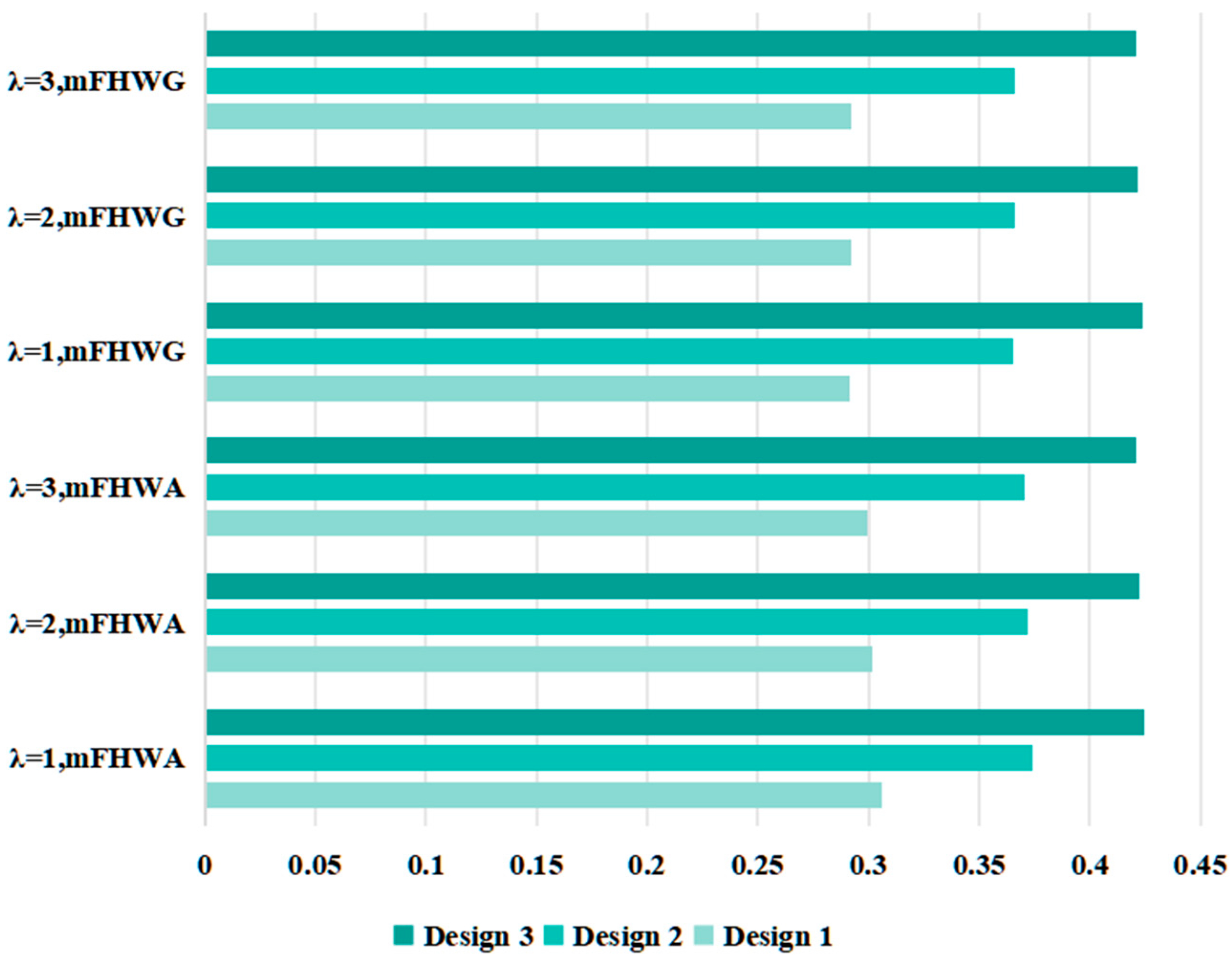
Operators	Score Values	Ranking
$\mathsf{\lambda }=1$, mFHWA	$\mathrm{S}\left({\tilde{\mathfrak{Z}}}_1\right)=0.3058$$, \mathrm{S}\left({\tilde{\mathfrak{Z}}}_2\right)=0.3740$$, \mathrm{S}\left({\tilde{\mathfrak{Z}}}_3\right)=0.4245$	${\mathfrak{D}}_3$$> {\mathfrak{D}}_2$$> {\mathfrak{D}}_1$
$\mathsf{\lambda }=2$, mFHWA	$\mathrm{S}\left({\tilde{\mathfrak{Z}}}_1\right)=0.30$$20, \mathrm{S}\left({\tilde{\mathfrak{Z}}}_2\right)=0.371$$8, \mathrm{S}\left({\tilde{\mathfrak{Z}}}_3\right)=0.4224$	${\mathfrak{D}}_3$$> {\mathfrak{D}}_2$$> {\mathfrak{D}}_1$
$\mathsf{\lambda }=3$, mFHWA	$\mathrm{S}\left({\tilde{\mathfrak{Z}}}_1\right)=0.299$$7, \mathrm{S}\left({\tilde{\mathfrak{Z}}}_2\right)=0.370$$4, \mathrm{S}\left({\tilde{\mathfrak{Z}}}_3\right)=0.421$2	${\mathfrak{D}}_3$$> {\mathfrak{D}}_2$$> {\mathfrak{D}}_1$
$\mathsf{\lambda }=1$, mFHWG	$\mathrm{S}\left({\tilde{\mathfrak{Z}}}_1\right)=0.2916$$, \mathrm{S}\left({\tilde{\mathfrak{Z}}}_2\right)=0.3654$$, \mathrm{S}\left({\tilde{\mathfrak{Z}}}_3\right)=0.4235$	${\mathfrak{D}}_3$$> {\mathfrak{D}}_2$$> {\mathfrak{D}}_1$
$\mathsf{\lambda }=2$, mFHWG	$\mathrm{S}\left({\tilde{\mathfrak{Z}}}_1\right)=0.2919$$, \mathrm{S}\left({\tilde{\mathfrak{Z}}}_2\right)=0.365$$7, \mathrm{S}\left({\tilde{\mathfrak{Z}}}_3\right)=0.4217$	${\mathfrak{D}}_3$$> {\mathfrak{D}}_2$$> {\mathfrak{D}}_1$
$\mathsf{\lambda }=3$, mFHWG	$\mathrm{S}\left({\tilde{\mathfrak{Z}}}_1\right)=0.2918$$, \mathrm{S}\left({\tilde{\mathfrak{Z}}}_2\right)=0.365$$7, \mathrm{S}\left({\tilde{\mathfrak{Z}}}_3\right)=0.4206$	${\mathfrak{D}}_3$$> {\mathfrak{D}}_2$$> {\mathfrak{D}}_1$

and

Table 11. Results of 2TLmFHWA and 2TLmFHWG operators.

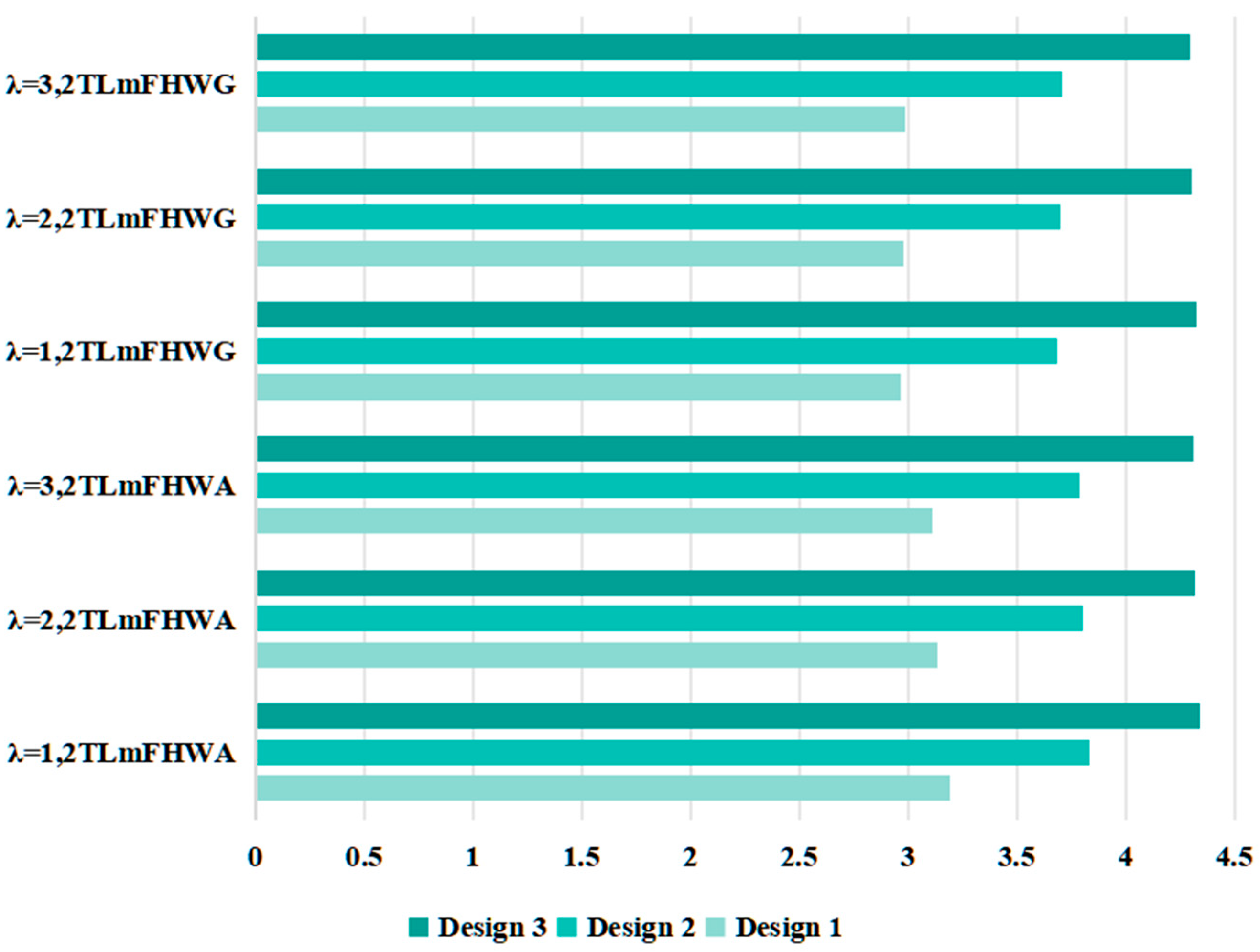
Operators	Score Values	Ranking
$\mathsf{\lambda }=1$, 2TLmFHWA	$\mathrm{S}\left({\tilde{\mathfrak{Z}}}_1\right)=\left(s_3,0.1963\right)$$, \mathrm{S}\left({\tilde{\mathfrak{Z}}}_2\right)=\left(s_4,-0.1687\right)$$, \mathrm{S}\left({\tilde{\mathfrak{Z}}}_3\right)=\left(s_4,0.3428\right)$	${\mathfrak{D}}_3$$> {\mathfrak{D}}_2$$> {\mathfrak{D}}_1$
$\mathsf{\lambda }=2$, 2TLmFHWA	$\mathrm{S}\left({\tilde{\mathfrak{Z}}}_1\right)=\left(s_3,0.1375\right)$$, \mathrm{S}\left({\tilde{\mathfrak{Z}}}_2\right)=\left(s_4,-0.1994\right)$$, \mathrm{S}\left({\tilde{\mathfrak{Z}}}_3\right)=\left(s_4,0.3182\right)$	${\mathfrak{D}}_3$$> {\mathfrak{D}}_2$$> {\mathfrak{D}}_1$
$\mathsf{\lambda }=3$, 2TLmFHWA	$\left({\tilde{\mathfrak{Z}}}_1\right)=\left(s_3,0.1094\right)$$, \mathrm{S}\left({\tilde{\mathfrak{Z}}}_2\right)=\left(s_4,-0.2138\right)$$, \mathrm{S}\left({\tilde{\mathfrak{Z}}}_3\right)=\left(s_4,0.3069\right)$	${\mathfrak{D}}_3$$> {\mathfrak{D}}_2$$> {\mathfrak{D}}_1$
$\mathsf{\lambda }=1$, 2TLmFHWG	$\mathrm{S}\left({\tilde{\mathfrak{Z}}}_1\right)=\left(s_3,-0.0385\right)$$, \mathrm{S}\left({\tilde{\mathfrak{Z}}}_2\right)=\left(s_4,-0.3108\right)$$, \mathrm{S}\left({\tilde{\mathfrak{Z}}}_3\right)=\left(s_4,0.3239\right)$	${\mathfrak{D}}_3$$> {\mathfrak{D}}_2$$> {\mathfrak{D}}_1$
$\mathsf{\lambda }=2$, 2TLmFHWG	$\mathrm{S}\left({\tilde{\mathfrak{Z}}}_1\right)=\left(s_3,-0.0221\right)$$, \mathrm{S}\left({\tilde{\mathfrak{Z}}}_2\right)=\left(s_4,-0.3005\right)$$, \mathrm{S}\left({\tilde{\mathfrak{Z}}}_3\right)=\left(s_4,0.3043\right)$	${\mathfrak{D}}_3$$> {\mathfrak{D}}_2$$> {\mathfrak{D}}_1$
$\mathsf{\lambda }=3$, 2TLmFHWG	$\mathrm{S}\left({\tilde{\mathfrak{Z}}}_1\right)=\left(s_3,-0.0125\right)$$, \mathrm{S}\left({\tilde{\mathfrak{Z}}}_2\right)=\left(s_4,-0.2929\right)$$, \mathrm{S}\left({\tilde{\mathfrak{Z}}}_3\right)=\left(s_4,0.2957\right)$	${\mathfrak{D}}_3$$> {\mathfrak{D}}_2$$> {\mathfrak{D}}_1$

. We visualized the crisp scores of every design obtained using all operators, as shown in Figure 3 and Figure 4.

We compared four aggregation operators based on m-polar fuzzy sets and their extensions, and the results were consistent across all methods, demonstrating the robustness and stability of our proposed approach. However, mFHWA and mFHWG operators [20] did not account for the uncertainty introduced by linguistic variables, which is critical in scenarios where evaluations are inherently imprecise and expressed in linguistic terms. On the other hand, 2TLmFHWA and 2TLmFHWG operators [21] failed to incorporate DMs’ confidence levels in their evaluations, which is essential for accurately reflecting the reliability and trustworthiness of the provided assessments.

These considerations are critical in the context of adaptive product design evaluation. Adaptive designs often involve multiple dynamic attributes that evolve, requiring decision-making frameworks to effectively handle temporal variability and inherent uncertainty [1,2,3]. Linguistic variables are commonly used to describe qualitative attributes, such as usability or comfort, making the ability to model their uncertainty essential for accurate evaluations. Furthermore, DMs’ confidence levels provide a vital layer of insight [26], ensuring that evaluations are aggregated and weighted according to their reliability.

By integrating these factors, our mLZN-based method addresses key challenges in evaluating adaptive product designs, where precise and trustworthy assessments are crucial for selecting the most effective and sustainable solutions. This comprehensive approach ensures that the decision-making process is robust, adaptable, and aligned with the complexities of real-world design evaluation scenarios, solidifying the relevance and superiority of our method.

6. Conclusions

In this study, we developed the first dynamic evaluation framework specifically designed for the conceptual design of adaptive products. By integrating the strengths of mFS and LZN, we proposed the mLZN. This novel approach addresses the dynamic nature of product attributes and the uncertainty inherent in DM evaluations. Our framework fills a critical gap in existing MAGDM methodologies, which often overlook temporal variability and decision-maker confidence levels in dynamic scenarios.

We designed the mLZN framework to include operational rules, scoring, ranking methods, and aggregation operators, such as the mLZNWA and mLZNWG. These tools enable us to perform robust and flexible evaluations of dynamic attributes across multiple periods. We validated our framework through a case study on adaptive furniture design for children, demonstrating its capability to dynamically capture and evaluate key design attributes, including safety, ease of use, fun, and comfort. Through sensitivity and comparative analyses, we further confirmed the robustness and reliability of our approach under various conditions and scenarios.

While our proposed framework demonstrates significant potential, certain limitations warrant further exploration. One limitation of the current mLZN framework is its computational complexity, which can increase significantly as the number of attributes, periods, or decision-makers grows. Future work could explore efficient computational techniques or approximation algorithms to address this issue. Another limitation lies in the reliance on DMs’ linguistic evaluations and confidence levels, which may introduce subjectivity and affect the robustness of the results. Future enhancements to this framework could integrate knowledge-driven approaches, such as rule-based reasoning or expert-defined knowledge bases [52], to better capture the nuanced aspects of adaptiveness. Such methods could complement the fuzzy logic-based evaluation by adding domain-specific insights. The insights gained from applying the mLZN framework to adaptive furniture design can inspire its application in other domains. For instance, the framework’s ability to model dynamic changes over time and incorporate DMs’ confidence levels makes it well suited for problems involving evolving attributes, such as healthcare diagnostics or energy management systems.

References

- Saad, M.; Xue, D. Optimization to identify the adapted product design and product adaptation process with initial evaluation of information quality in branches of AND-OR tree based on information entropy. Adv. Eng. Inform. 2024, 62, 102649. [Google Scholar] [CrossRef]
- Gu, P.; Hashemian, M.; Nee, A.Y.C. Adaptable design. CIRP Ann.-Manuf. Technol. 2004, 53, 539–557. [Google Scholar] [CrossRef]
- Gu, P.; Xue, D.; Nee, A.Y.C. Adaptable design: Concepts, methods, and applications. Proc. Inst. Mech. Eng. Part B J. Eng. Manuf. 2009, 223, 1367–1387. [Google Scholar] [CrossRef]
- Nikander, J.B.; Liikkanen, L.A.; Laakso, M. The preference effect in design concept evaluation. Des. Stud. 2014, 35, 473–499. [Google Scholar] [CrossRef]
- Martinez, M.; Xue, D. A modular design approach for modeling and optimization of adaptable products considering the whole product utilization spans. Proc. Inst. Mech. Eng. Part C J. Mech. Eng. Sci. 2017, 232, 1146–1164. [Google Scholar] [CrossRef]
- Han, X.; Li, R.; Wang, J.; Qin, S.; Ding, G. Identification of key design characteristics for complex product adaptive design. Int. J. Adv. Manuf. Technol. 2018, 95, 1215–1231. [Google Scholar] [CrossRef]
- Schuh, G.; Prote, J.P.; Luckert, M.; Basse, F.; Thomson, V.; Mazurek, W. Adaptive Design of Engineering Change Management in Highly Iterative Product Development. Procedia CIRP 2018, 70, 72–77. [Google Scholar] [CrossRef]
- Jing, L.; Zhang, H.; Dou, Y.; Feng, D.; Jia, W.; Jiang, S. Conceptual design decision-making considering multigranularity heterogeneous evaluation semantics with uncertain beliefs. Expert Syst. Appl. 2024, 244, 122963. [Google Scholar] [CrossRef]
- Aydoğan, S.; Günay, E.E.; Akay, D.; Okudan Kremer, G.E. Concept design evaluation by using Z-axiomatic design. Comput. Ind. 2020, 122, 103278. [Google Scholar] [CrossRef]
- Irvanizam, I.; Zi, N.N.; Zuhra, R.; Amrusi, A.; Sofyan, H. An Extended MABAC Method Based on Triangular Fuzzy Neutrosophic Numbers for Multiple-Criteria Group Decision Making Problems. Axioms 2020, 9, 104. [Google Scholar] [CrossRef]
- Mondal, K.; Pramanik, S.; Giri, B.C.; Smarandache, F. NN-Harmonic Mean Aggregation Operators-Based MCGDM Strategy in a Neutrosophic Number Environment. Axioms 2018, 7, 12. [Google Scholar] [CrossRef]
- Lin, C.; Twu, C. Combination of a fuzzy analytic hierarchy process (FAHP) with the Technique for Order Preference by Similarity to Ideal Solution (TOPSIS) for fashion design scheme evaluation. Text. Res. J. 2012, 82, 1065–1074. [Google Scholar] [CrossRef]
- Geng, R.; Ji, Y.; Qu, S.; Wang, Z. Data-driven product ranking: A hybrid ranking approach. J. Intell. Fuzzy Syst. 2023, 44, 6573–6592. [Google Scholar] [CrossRef]
- Rashid, T.; Ali, A.; Guirao, J.L.G.; Valverde, A. Comparative Analysis of Hybrid Fuzzy MCGDM Methodologies for Optimal Robot Selection Process. Symmetry 2021, 13, 839. [Google Scholar] [CrossRef]
- Akram, M.; Wasim, F.; Karaaslan, F. MCGDM with complex Pythagorean fuzzy -soft model. Expert Syst. 2021, 38, e12783. [Google Scholar] [CrossRef]
- Tiwari, V.; Jain, P.K.; Tandon, P. Product design concept evaluation using rough sets and VIKOR method. Adv. Eng. Inf. 2016, 30, 16–25. [Google Scholar] [CrossRef]
- Jing, L.; Yao, J.; Gao, F.; Li, J.; Peng, X.; Jiang, S. A rough set-based interval-valued intuitionistic fuzzy conceptual design decision approach with considering diverse customer preference distribution. Adv. Eng. Inf. 2021, 48, 101284. [Google Scholar] [CrossRef]
- Chen, J.; Li, S.; Ma, S.; Wang, X. m-Polar Fuzzy Sets: An Extension of Bipolar Fuzzy Sets. Sci. World J. 2014, 2014, 416530. [Google Scholar] [CrossRef]
- Zhang, W.R. (Yin) (Yang) bipolar fuzzy sets. In Proceedings of the 1998 IEEE International Conference on Fuzzy Systems Proceedings, IEEE World Congress on Computational Intelligence (Cat. No.98CH36228), Anchorage, AK, USA, 4–9 May 1998; Volume 831, pp. 835–840. [Google Scholar]
- Waseem, N.; Akram, M.; Alcantud, J.C.R. Multi-Attribute Decision-Making Based on m-Polar Fuzzy Hamacher Aggregation Operators. Symmetry 2019, 11, 1498. [Google Scholar] [CrossRef]
- Akram, M.; Noreen, U.; Ali Al-Shamiri, M.M. Decision Analysis Approach Based on 2-Tuple Linguistic m-Polar Fuzzy Hamacher Aggregation Operators. Discret. Dyn. Nat. Soc. 2022, 2022, 6269115. [Google Scholar] [CrossRef]
- Mondal, A.; Roy, S.K.; Zhan, J. A reliability-based consensus model and regret theory-based selection process for linguistic hesitant-Z multi-attribute group decision making. Expert Syst. Appl. 2023, 228, 120431. [Google Scholar] [CrossRef]
- Jia, Q.; Hu, J. A novel method to research linguistic uncertain Z-numbers. Inf. Sci. 2022, 586, 41–58. [Google Scholar] [CrossRef]
- Zhu, G.-N.; Hu, J.; Qi, J.; Gu, C.-C.; Peng, Y.-H. An integrated AHP and VIKOR for design concept evaluation based on rough number. Adv. Eng. Inf. 2015, 29, 408–418. [Google Scholar] [CrossRef]
- Zadeh, L.A. A Note on Z-numbers. Inf. Sci. 2011, 181, 2923–2932. [Google Scholar] [CrossRef]
- Liu, Q.; Chen, J.; Wang, W.; Qin, Q. Conceptual design evaluation considering confidence based on z-ahp-topsis method. Appl. Sci. 2021, 11, 7400. [Google Scholar] [CrossRef]
- Liu, Q.; Chen, J.; Yang, K.; Liu, D.; He, L.; Qin, Q.; Wang, Y. An integrating spherical fuzzy AHP and axiomatic design approach and its application in human–machine interface design evaluation. Eng. Appl. Artif. Intell. 2023, 125, 106746. [Google Scholar] [CrossRef]
- Jing, L.; Fan, X.; Feng, D.; Lu, C.; Jiang, S. A patent text-based product conceptual design decision-making approach considering the fusion of incomplete evaluation semantic and scheme beliefs. Appl. Soft Comput. 2024, 157, 111492. [Google Scholar] [CrossRef]
- Ali, G.; Sarwar, M.; Nabeel, M. Novel group decision-making method based on interval-valued m-polar fuzzy soft expert information. Neural Comput. Appl. 2023, 35, 22313–22340. [Google Scholar] [CrossRef]
- Rahman, Z.U.; Ali, G.; Asif, M.; Chen, Y.; Abidin, M.Z.U. Identification of desalination and wind power plants sites using m-polar fuzzy Aczel–Alsina aggregation information. Sci. Rep. 2024, 14, 409. [Google Scholar] [CrossRef]
- Sivakumar, M.; Basarıya, A.R.R.; Senthil, M.; Vetriselvi, T.; Raja, G.; Rajavarman, R. Transforming Arabic Text Analysis: Integrating Applied Linguistics with m-Polar Neutrosophic Set Mood Change and Depression on Social Media. Int. J. Neutrosophic Sci. 2025, 25, 313–324. [Google Scholar] [CrossRef]
- Akram, M.; Noreen, U.; Deveci, M. An outranking method for optimizing anti-aircraft missile system with 2-tuple linguistic m-polar fuzzy data. Eng. Appl. Artif. Intell. 2024, 132, 107923. [Google Scholar] [CrossRef]
- Akram, M.; Siddique, S.; Alcantud, J.C.R. Connectivity indices of m-polar fuzzy network model, with an application to a product manufacturing problem. Artif. Intell. Rev. 2023, 56, 7795–7838. [Google Scholar] [CrossRef]
- Bera, S.; Muhiuddin, G.; Pal, M. Facility location problem using the concept of double domination in m-polar interval-valued fuzzy graph. J. Intell. Fuzzy Syst. 2023, 45, 7713–7726. [Google Scholar] [CrossRef]
- Akram, M.; Sultan, M.; Deveci, M. An integrated multi-polar fuzzy N-soft preference ranking organization method for enrichment of evaluations of the digitization of global economy. Artif. Intell. Rev. 2024, 57, 74. [Google Scholar] [CrossRef]
- Alshayea, M.A.; Alsager, K.M. m-polar Q-hesitant anti-fuzzy set in BCK/BCI-algebras. Eur. J. Pure Appl. Math. 2024, 17, 338–355. [Google Scholar] [CrossRef]
- Kausar, R.; Riaz, M.; Yasin, Y.; Deveci, M.; Pamucar, D. Measuring efficiency of retrieval algorithms with Schweizer-Sklar information aggregation. Inf. Sci. 2023, 647, 119438. [Google Scholar] [CrossRef]
- Jia, Q.; Hu, J.; Safwat, E.; Kamel, A. Polar coordinate system to solve an uncertain linguistic Z-number and its application in multicriteria group decision-making. Eng. Appl. Artif. Intell. 2021, 105, 104437. [Google Scholar] [CrossRef]
- Li, D. A linguistic Z-number-based dual perspectives information volume calculation method for driving behavior risk evaluation. Expert Syst. Appl. 2024, 257, 124992. [Google Scholar] [CrossRef]
- Chen, H.; Jia, Q.; Huang, W.; Shi, J.; Safwat, E. Combination of linguistic Z-numbers and IF-THEN rules based on rectangular coordinate system. J. Intell. Fuzzy Syst. 2023, 45, 1251–1268. [Google Scholar] [CrossRef]
- Wang, J.Q.; Cao, Y.X.; Zhang, H.Y. Multi-Criteria Decision-Making Method Based on Distance Measure and Choquet Integral for Linguistic Z-Numbers. Cogn. Comput. 2017, 9, 827–842. [Google Scholar] [CrossRef]
- Chai, J.; Su, Y.; Lu, S. Linguistic Z-number preference relation for group decision making and its application in digital transformation assessment of SMEs. Expert Syst. Appl. 2023, 213, 118749. [Google Scholar] [CrossRef]
- Tao, Z.; Liu, X.; Chen, H.; Liu, J.; Guan, F. Linguistic Z-number fuzzy soft sets and its application on multiple attribute group decision making problems. Int. J. Intell. Syst. 2020, 35, 105–124. [Google Scholar] [CrossRef]
- Liu, Y.; Yang, Z.; He, J.; Li, G.; Zhong, Y. Linguistic q-rung orthopair fuzzy Z-number and its application in multi-criteria decision-making. Eng. Appl. Artif. Intell. 2024, 133, 108432. [Google Scholar] [CrossRef]
- Fan, J.; Zhu, Q.; Wu, M. Failure mode and effect analysis using VIKOR method based on interval-valued linguistic Z-numbers. J. Intell. Fuzzy Syst. 2024, 46, 1183–1199. [Google Scholar] [CrossRef]
- Kumar, K.; Chen, S.-M. Group decision making based on linguistic intuitionistic fuzzy Yager weighted arithmetic aggregation operator of linguistic intuitionistic fuzzy numbers. Inf. Sci. 2023, 647, 119228. [Google Scholar] [CrossRef]
- Zichun, C.; Penghui, L.; Zheng, P. An approach to multiple attribute group decision making based on linguistic intuitionistic fuzzy numbers. Int. J. Comput. Intell. Syst. 2015, 8, 747–760. [Google Scholar] [CrossRef]
- Wang, J.-q.; Wu, J.-t.; Wang, J.; Zhang, H.-y.; Chen, X.-h. Interval-valued hesitant fuzzy linguistic sets and their applications in multi-criteria decision-making problems. Inf. Sci. 2014, 288, 55–72. [Google Scholar] [CrossRef]
- Kumar, K.; Chen, S.-M. Multiple attribute group decision making based on advanced linguistic intuitionistic fuzzy weighted averaging aggregation operator of linguistic intuitionistic fuzzy numbers. Inf. Sci. 2022, 587, 813–824. [Google Scholar] [CrossRef]
- Song, C.; Wang, J.-Q.; Li, J.-B. New Framework for Quality Function Deployment Using Linguistic Z-Numbers. Mathematics 2020, 8, 224. [Google Scholar] [CrossRef]
- Wen, X.; Pashkevych, K.L. Analysis of furniture design for growing children based on physiological changes in children. Art Des. 2023, 3, 57–67. [Google Scholar] [CrossRef]
- Cheng, C.; Ding, W.; Xiao, F.; Pedrycz, W. A Majority Rule-Based Measure for Atanassov-Type Intuitionistic Membership Grades in MCDM. IEEE Trans. Fuzzy Syst. 2022, 30, 121–132. [Google Scholar] [CrossRef]